Abstract
This paper focuses on the valuation and hedging of gas storage facilities, using a spot-based valuation framework coupled with a financial hedging strategy implemented with futures contracts. The contributions of this paper are two-fold. Firstly, we propose a model that unifies the dynamics of the futures curve and spot price, and accounts for the main stylized facts of the US natural gas market such as seasonality and the presence of price spikes in the spot market. Secondly, we evaluate the associated model risk, and show not only that the valuation is strongly dependent upon the dynamics of the spot price, but more importantly that the hedging strategy commonly used in the industry leaves the storage operator with significant residual price risk.
MSC:
91G10; 91G60; 91G70; 91G80
JEL Classification:
C4; C5; C6; C8; G11; G13; G17
1. Introduction
Natural Gas (NG) storage units are used to reconcile the variable seasonal demand for gas with the more constant rate of natural gas production. These gas storage facilities are mainly owned by distribution companies which use them for system supply regulation, and for reducing the risk of shortages. In fact, regulation requires that local distribution companies own storage units, in order to secure their gas supply and to be able to meet any sudden increase in demand or any disruption in the pipeline transportation system.
Traditionally, say prior to about 2005, gas storage units were valued using a discounted cash flow, also called intrinsic, method. The idea was to project an optimal schedule of injections and withdrawals, using the term structure of future prices, and compute the corresponding discounted cash flow, which provided a lower bound to the storage value. Following this strategy, the storage manager observed the futures curve at the beginning of the storage contract and bought/sold futures contracts, thereby determining once and for all the complete schedule of injection and withdrawals; essentially, this lead to buying cheap summer futures and selling expensive winter futures and the corresponding storage value greatly depended upon the summer-winter spread.
Since the late 2000s, however, the seasonal spread has consistently shrunk, putting into question the futures-based methodology. The 2011 State of the Markets report, issued by the US Federal Energy Regulatory Commission (FERC 2012), noticed the following: We have also seen a decline in the seasonal difference between winter and summer natural gas prices. Falling seasonal spreads reflect increased production and storage capacity, as well as greater year-round use of natural gas by power generators. This decline has developed over the past several years and we expect the trend to continue.
This narrowing winter/summer spread was mainly due to two factors that simultaneously put a downward pressure on winter gas prices and an upward pressure on summer prices. The first factor was the recent surge in non conventional shale gas supply, with geographical locations that were closer to gas consumption areas. The main effect of this new abundant supply was a downward pressure on winter prices. The second factor is related to power consumption by cooling systems during summer periods and the growing use of natural gas as a fuel for electricity generation. This puts an upward pressure on summer gas prices. The combination of these two factors had the logical consequence of narrowing the seasonal spreads between winter and summer prices, diminishing the intrinsic value of gas storage units. The phenomenon has even amplified over time to the point that, as of January 2018, the maximum summer-winter spread is about 50 cents.
Static strategies based on futures contracts were no longer adequate to monetize the value of gas storage facilities; they even sometimes failed to recover the operating expenses. This motivated an interest in dynamic strategies that took advantage of the real options embedded in gas storage facilities. These methods are called extrinsic because they take into account the time value of the embedded calendar spread options. As intended, they evaluated the storage units, in particular the units with a high injection/withdrawal rate, at a much higher value than the traditional intrinsic value. However, switching from an intrinsic to an extrinsic valuation method was a major paradigm shift in risk management, and this for two reasons:
- The extrinsic method relies on a precise model of the dynamics of the Natural Gas term structure, and in particular on the modeling of correlation between futures contracts, and between the futures prices and the cash price of Natural Gas. Contrast this with the intrinsic method, which takes the term structure as a given, and does not require any model of the price dynamics.
- The traditional intrinsic method assigned to the storage unit a value that could be recovered for certain by implementing a static trading strategy in Natural Gas Futures. In contrast, the extrinsic method, by analogy with financial options, determines the expected discounted value of future cash flows. The analogy with a financial option stops here however, because, contrary to an option on a stock, for example, the hedging strategy is far from being as readily available.
The purpose of this paper is to stress the magnitude of this paradigm shift, and its contributions are two-fold.
- Firstly, we provide a model of the dynamics of the NG market, that incorporates all the features relevant for the evaluation of options embedded in a storage unit. To this end, we introduce a new modeling framework that unifies the dynamics of the futures curve and spot price, and is consistent with the two stylized facts that are essential to the gas storage valuation problem: price seasonality and spot price spikes.
- Secondly, we attempt to quantify the model uncertainty inherent to the extrinsic method. We highlight in particular the significant sensitivity of gas storage value to the specification and estimation of the spot model. This result puts into perspective the extensive literature on gas storage valuation, and calls for a more careful assessment of the model risk inherent to these valuations. We conclude that in the current state of the art, a significant portion of the extrinsic value cannot be monetized in a reliable manner.
Summary of Findings
We find that the switch from an intrinsic to an extrinsic valuation method introduces a significant level of model risk in the pricing and risk management of storage units. We have identified a model formulation for the dynamics of the asset price that somehow mitigates this risk, but model risk still remain a full order of magnitude larger than for standard financial options. In this context, the extrinsic method, should be understood as providing a broad indicator of value rather than a firm price. This puts into perspective the concentration of effort in the literature on the specification of an optimal valuation strategy. More attention should probably be devoted to the discussion of modeling assumptions.
After this introduction the paper is organized as follows. In Section 2, we provide a summary of the literature with respect to both the storage valuation methods and the modeling of the dynamics of the Natural Gas term structure. Next, we introduce in Section 3 our model for the price process, and motivate our modeling choices by an investigation of the stylized facts observed in the Natural Gas market. In Section 4 we use our models to price typical storage facilities, using both the extrinsic and intrinsic methods. Section 5 is devoted to the measure of model risk in extrinsic methods. We introduce two natural model risk measures to quantify the sensitivity of a class of models with respect to the parameters; those risk measures are computed in several test cases.
2. Survey of Relevant Literature
In this section, we summarize the existing literature on the two topics of interest for our inquiry, which are the methodology for pricing and hedging a gas storage facility on one hand, and the dynamics of the term structure of gas price on the other hand.
2.1. Valuation and Hedging of a Gas Storage Unit
The problem of valuing gas storage units has been discussed from many angles in the literature, yielding different approaches and numerical methods. Leasing a gas storage unit is equivalent to paying for the right, but not the obligation, to inject or withdraw gas from the unit, and the operator’s goal is obviously to optimize the exercise of that right by injecting or withdrawing gas from the unit and, at the same time, trading gas on the spot and/or futures market. All these decisions have to be made under many operational constraints, such as maximal and minimal volume in storage, and limited injection and withdrawal rates. Methods for determining the optimal operating policy—an therefore the value of the storage—fall in two broad categories: the intrinsic methods and the extrinsic methods, which are described next.
Remark 1.
For simplicity, in the rest of this article, we suppose the discount interest rate to vanish, and consider the problem specification in a time discrete setting.
2.1.1. Gas Storage Problem Formulation
We consider a gas storage facility with technical constraints (either physical or regulatory) on the volume of stored gas, and i.e., at all time, the volume of stored gas V should verify .
We assume a discrete set of dates for with . At each date and starting from a volume , the user has the possibility to make one of three decisions: either inject gas at rate of , or withdraw gas at rate of or take no action. We denote by the decision at time , and write (resp. , ) if the decision is injecting gas at rate (resp. withdrawing gas at rate , no action).
If the user follows a strategy , then the volume of gas in storage is given by the iteration
Denoting the spot price of gas, the generated cash flow (positive when withdrawing gas, negative when injecting) is given by
In general, the maximum injection and withdrawal rates ( and ) are functions of the amount of gas in storage. However, without loss of generality, we assume for simplicity that these rates are constant. In Table 1 we summarize the possible decisions and their consequences on gas volume and generated cash flow.

Table 1.
Possible decisions.
According to the intrinsic method, a trading strategy is determined once and for all at the beginning of the lease. In order to determine the optimal futures positions, a linear optimization problem is solved, with constraints imposed by the specifics of the storage unit (Eydeland and Krzysztof 2002). Assume that N futures contracts, expiring at times , are available for trading, and let be the price at t of a futures contract expiring at time . The optimization problem amounts to finding the number of futures contracts to buy or sell at the start of the lease, and can be expressed as follows:
The cash flow corresponding to the optimal solution can be obtained for certain by implementing the trading strategy at the start of the lease. The subsequent evolution of the futures curve will not have any impact on the cash flow.
This static methodology was extended by Gray and Khandelwal (2004) to the rolling intrinsic valuation, to take advantage of the changing shape of the futures curve. According to this variant, optimal futures positions are chosen at the beginning of the storage contract, but when the futures curve moves away from its initial shape, new optimal futures positions are recalculated, and the portfolio is rebalanced if this is found to be profitable.
Prompted by shrinking winter-summer spreads, it was soon recognized that this approach failed to capture an important component of the storage value, related to the uncertainty of future prices, and to operator’s ability to modify his policy to take advantage of new information. The methods that capture the value of these options are called extrinsic methods, and they involve the resolution of a constrained stochastic control problem, which is now described, using the notations of Warin (2012). The goal of the storage operator is to find a strategy u maximizing the expected cumulative cash flows. We denote this optimal value by , which is the solution of the following problem:
From Table 1, we recall that only depends on and . To emphasize this fact, if , we also express by .
At time t, for and with current volume level v, the (optimal) value for gas storage will be of course denoted by . The dynamic programming principle implies
The classic way to solve this problem numerically is to use Monte Carlo simulations, combined with the Longstaff and Schwartz (2001) algorithm, which approximates the above conditional expectation, using a regression technique. This backward algorithm yields an estimate of the optimal strategy ; we refer the reader to Boogert and De Jong (2008) for a detailed description of the algorithm and its implementation.
The optimal value for , however, is not used as such: having determined an optimal strategy function of time, of the amount of gas in storage and of the forward curve, the storage value is determined by a forward algorithm that involves two steps:
- simulate paths for the forward curve and the spot price;
- along each path, apply the optimal decision rule and determine the corresponding cash flow.
The expected total discounted cash flow over the paths is an estimate of , the optimal extrinsic value (EV) of the storage unit.
Whereas the intrinsic method provide a price that can be obtained for certain through a trading strategy in the futures market, a manager who follows the optimal strategy on a single path is not assured to recover the expected value . There will certainly be a discrepancy between the realized cumulative cash flows on a given path and the expected value. Hence, it is crucial for the storage manager to reduce the variance of the cumulative cash flows, which is a random variable. As we will explain in the next section, this can be achieved by conducting a financial hedging strategy, based on futures contracts.
2.1.2. Financial Hedging Strategy
The optimal operating strategy will be combined with additional financial trades, so that the expectation of the related cumulative wealth generated by both physical and financial operations is still , but its variance (or some other risk criterion) is reduced. This additional financial hedging strategy plays a role analogous to control variates in the variance reduction of Monte Carlo simulations, as it preserves the expected value and reduces its variance. In order to reduce the variance of a Monte Carlo estimator of a r.v. Y, one adds to it a mean zero control variate, which is highly (negatively) correlated to Y. Since futures contracts are the most liquid assets in the natural gas market, and are strongly correlated to the spot price, they form an ideal hedging instrument. In fact, although a futures contract price does not converge to the spot price, when the time to maturity goes to zero, the correlation between the prompt contract (for example) and the spot price is very high, and often the two contracts move in the same direction. The basic idea of a financial hedging strategy is to add to the physical spot trading, a strategy of buying and selling, at a trading date , a quantity of futures contracts for . Logically, those quantities will depend on the spot and futures prices, S and , but also on the current volume level.
If the gas storage manager follows such a hedging strategy, in addition to the spot physical trading, then the cumulative cash flows of the combined strategies is:
Because the futures contract stops trading after its expiration date , we use the convention .
Since the futures price process is a martingale under the risk neutral probability, we have
Hence, the expectation of this hedging strategy is null i.e.,
Consequently, following the optimal spot strategy in parallel with a futures hedging portfolio gives the same cash flows in expectation, but very likely with lower variance.
The specification of such a hedging strategy will of course depend on the nature of the relation between the spot price and the futures curve.
A heuristic strategy that is widely used in the industry is to take the quantity of futures to be equal to the conditional expectation of volume to be exercised during the delivery period of the futures contract, conditional on the information at . More precisely, the heuristic delta is equal to the -conditional expectation
A modification of this heuristic delta, using the concept of tangent process has been introduced by Warin (2012): If we assume that the prompt converges towards the spot, then we can write
which yields the modified heuristic delta :
We emphasize that the definition of these two hedging strategies is based on heuristic reasoning. Therefore, the hedging will not be perfect and a residual risk still remains; still, the numerical experiments of Section 4 show that this financial hedging strategy does yield a significant reduction in the cash flows uncertainty of the spot trading strategy.
Generally, the problem of gas storage unit valuation has been studied from the angle of numerical methods, and not much interest has been paid to the modeling of the underlying price processes themselves and their effects on the final outcome of the calculation, although these modeling choices, as we shall see, have a profound impact on the valuation and hedging decisions.
2.2. The Dynamics of the Term Structure of Gas Price
Two modeling approaches may be found in the literature: the first approach consists in modeling the spot price by itself, with classical mean-reverting models, while a more recent approach attempts to model the dynamics of the entire term structure. We now describe in some details these two approaches, focusing on the effect of modeling decisions on the valuation of storage units.
2.2.1. Spot Price Processes
A very common framework consists in modeling the spot price as a mean-reverting process. For instance, Boogert and De Jong (2008) consider a one factor model for the spot price, which is calibrated to the initial futures curve. The price process S is given by
where W is a standard Brownian motion, is a time-dependent parameter, calibrated to the initial futures curve , provided by the market; the mean reversion parameter and the volatility are two positive constants.
As pointed out by Bjerksund et al. (2011), this framework has several drawbacks with respect to the goal of capturing the value of the gas storage. The calibration of the time-varying function is, as expected, quite unstable and gives unrealistic sensitivity of the spot dynamics, and hence of the gas storage value with respect to the initial futures curve.
More importantly, this spot modeling implies a dynamic where future contracts are perfectly correlated, and therefore does not open the possibility of a trading strategy involving spreads between futures contracts. Modeling the futures curve is indispensable in order to formulate the hedging strategies based on futures contracts. Finally, (10) does not account for price spikes, which may be an important source of storage value.
An enhancement of this model is proposed by Parsons (2013), who considers the following two-factor mean-reverting model:
where the spot price S follows a mean-reverting process, with a long-run mean which is itself a stochastic process reverting to a deterministic value .
While this model is more realistic than the one factor model, it still suffers from the instability of the deterministic function , and still does not include the possibility of spikes in the spot price. The author defines the futures contract price as the expectation of the spot price at maturity date T. We emphasize that this definition implies that natural gas is delivered at the futures expiration T; in reality, however, the delivery period spans an entire calendar month.
Finally, gas storage valuation has been studied by Safarov and Atkinson (2017) in the context of a spot price modeled by a time in-homogeneous exponential Lévy process, taking into account the seasonality, mean-reversion and price spikes with seasonal jump intensities.
2.2.2. Term Structure Models
Early models of commodities futures prices , such as the classical models of Gibson and Schwartz (1990) and Schwartz (1997), were obtained through conditional expectations of with respect to the current information at time t, where S is the spot price process. This process was linked to futures prices through additional, possibly stochastic, quantities such as convenience yield and interest rates. The approach has several drawbacks such as the difficulty of observing or estimating those quantities and the problem of fitting the initial curve .
Hence, a second generation of models was proposed to directly describe the futures curve, using multi-factor log-normal dynamics. For instance, Clewlow and Strickland (1999b) proposes a one-factor model for the futures curve; this was then extended by Clewlow and Strickland (1999a) to a multi-factor setting. A two-factor version of this model can be expressed as
where , and are positive constants, and and are two correlated Brownian motions. This model has the advantage of exactly fitting the initial futures curve, and the dependence of the volatility on the maturity parameter, i.e., it is of term-structure type; however it does not take into account the essential seasonality feature. Note that this model is an adaptation of the well-known Gabillon (1991) model, originally proposed for spot prices. A second approach, adopted by Warin (2012) is to model the entire term structure. The author considers a n-factor log-normal dynamics for the futures curve:
and assumes that the spot process is the limit of the futures contract price as time to maturity goes to zero; we would have . and by continuity the spot is given by . This allows the author to give formulae for the sensitivities of storage value with respect to futures contracts, and to provide a hedging strategy based on futures in parallel to the spot optimal trading strategy.
Unfortunately, this assumption does not conform to reality, since the spot price correspond to gas delivered the next day, while the futures is settled by rated delivery over an entire calendar month.
To summarize, the available research on storage valuation is based on models for the price processes that either do not capture important features of the spot process, or assume a convergence of the futures to the spot price that does not conform to reality. In contrast, we present next a joint, multi-factor model for the futures curve and the spot process. It captures the seasonality of the natural gas futures prices and the correlation between the spot and prompt prices. It also accounts for the presence of spikes in the spot price.
3. Modeling Framework for the Price Process
In order to motivate our model, we first present some stylized facts about the prices of natural gas, then present the model formulation and its estimation.
3.1. Natural Gas Stylized Facts
In this section, we highlight important stylized facts about natural gas markets that may influence the value of a storage unit. These properties are related to the demand and use of natural gas. In fact, the demand for natural gas for heating in cold periods of the year produces a seasonal price pattern, while unpredictable changes in weather can cause sudden shifts in gas prices. These facts are the two main sources of value for a gas storage unit, since the ownership of a storage facility enables one to take advantage of seasonality and price spikes.
As for all other commodities, the price of natural gas (NG) is influenced by its point of delivery. In this study, we will be interested in the United States market, specifically in a storage location near Henry Hub (Louisiana), which justifies the use of gas daily spot prices and the NYMEX natural gas futures as hedge instruments. One can buy natural gas in the spot market for next-day delivery, or in the futures market for rated delivery over a future period of one calendar month. The NYMEX futures market provides quotes for the next 72 monthly futures contracts, but only the first 24 or so are actively traded.
In what follows, will denote the spot price of natural gas at date t, and represent the futures contracts prices at t, for a set of maturities. We consider monthly spaced maturities, so every futures contract is related to a delivery month. Also, we denote by the price of prompt contract, i.e., the futures contract with the closest maturity to current time t. Natural gas prices are quoted in U.S. dollars per million British thermal units (MMBtu).
As mentioned above, the first main feature of natural gas prices is constituted by the presence of a seasonal component. We plot the NG futures curve for several dates in Figure 1 and observe a periodic winter increase in price, which are clearly due to the demand for heating during cold periods of the year. In addition to this traditional seasonal feature, the use of natural gas for electricity generation has created a second smaller increase during the summer period, related to the increasing demand for cooling. These expected patterns in natural gas prices are the first source of value for a storage unit, and have inspired the intrinsic strategy described in Section 1: buy gas for summer delivery and simultaneously sell gas for winter delivery. Store it in between, and you have locked a certain profit which is the summer-winter spread less the storage cost.
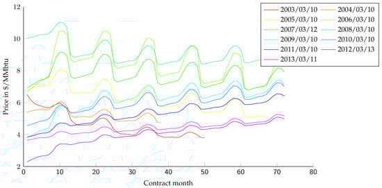
Figure 1.
Futures curve for NYMEX NG at different observation dates.
The second important aspect of natural gas prices is the presence of sudden moves due to unexpected imbalances between supply and demand, caused by such factors as unpredicted weather changes, disruptions in the supply chain, or poor anticipations of the global amount of gas in storage. Such events are almost instantaneously reflected in the spot dynamics, resulting in large price swings that are rapidly absorbed, however, by the storage capacities available in the market. These large and quickly absorbed jumps, commonly called spikes, can be viewed in Figure 2, which shows many sudden dislocations between spot and prompt prices.1 For example, we can notice a large spike in the spot price during late February 2003, when the natural gas price jumped by almost and in two successive days, then went down by and during the two following days. As noted by the US Federal Energy Regulatory Commission (FERC 2003), this spike in gas price was due to “physical market conditions leading to low supply and high demand for a short time.” The author also observed that “similar natural gas price spikes are possible when episodes of cold weather occur at times when storage inventories are limited”.
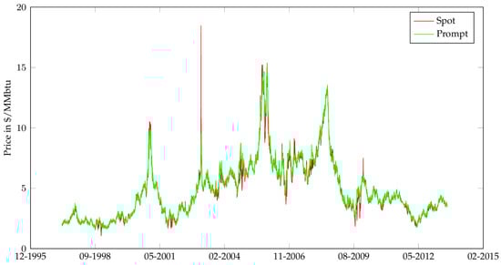
Figure 2.
Spot and prompt historical prices.
In our study, we detect spikes by identifying the outliers from the time series of the spread between the spot price and the prompt price given by ; we study separately the positive and negative spikes, since they reflect different market conditions. Positive spikes are often caused by unpredicted weather changes, such as a cold front or a heat wave. On the other hand, negative spikes are generally due to a poor anticipation of market-wide gas storage levels. In Figure 3 we plot the number of occurrences of negative and positive spikes during each month. We remark that the distribution of spikes is clearly dependent on their sign: most of the positive spikes happen during the winter months of January and February and the summer month of June, which can be explained by the occurrence of an unpredicted cold front or heat wave. On the other hand, negative spikes appear during the Fall. One plausible explanation is given by Mastrangelo (2007), which states: “October is the last month of the refill season. There may be increased competition from storage facilities looking to meet end-of-season refill goals as well as increased anticipation regarding the upcoming heating season”.
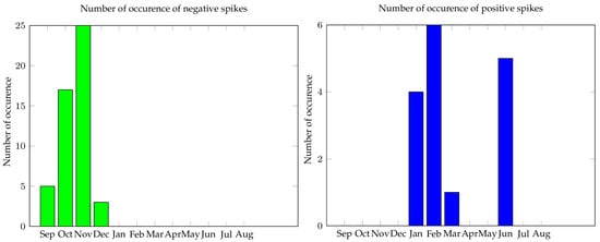
Figure 3.
Occurrences of spikes.
In order to take into account the stylized facts mentioned above, our futures model incorporates seasonality in the futures curve, and the spot model describes the existence of spikes and takes into account the correlation between spot and futures prices, through the prompt contract. To the best of our knowledge, these two facts have not yet been taken into account in the literature related to gas storage valuation, although, in our opinion, they constitute the two main sources of storage value.
In Section 3.1 we discussed the main stylized facts of natural gas prices, which are seasonality and spikes. We believe that the incorporation of these two features is essential in order to monetize these two sources of value. Also, we emphasize that it is crucial to use a modeling framework that combines spot and futures curve dynamics, and that accounts for the presence of a basis between the spot and prompt prices.
In Section 3.2, we introduce a two-factors model for the futures curve, with a seasonal component for instantaneous volatility. This parsimonious model has easy-to-interpret parameters and can be efficiently calibrated using futures curve historical data.
In Section 3.3, we discuss the spot price model: we consider two formulations, with a clear relation to the prompt contract. We also include spikes by means of a fast-reverting jump process, similar to a model by Hambly et al. (2009), which was applied to the electricity market.
3.2. Modeling the Futures Curve
Our framework slightly modifies Gabillon’s model, adding a seasonality component and introducing parameters that have an economical significance.
We will call it the Seasonal Gabillon two-factor model. It is formulated as
where and are two correlated Brownian motions, with . The letters L and S stand respectively for Long term and Short term; , and are positive constants. The function weights instantaneous volatility with a periodic behavior. It takes into account the winter seasonal peaks (resp. the secondary summer peak) by taking for example equal to January (resp. equal to August). There exist alternative ways to model price seasonality, e.g., in Nowotarski et al. (2013), in the context of electricity markets. The coefficients and quantify the winter and summer seasonal contribution to volatility: we expect the winter parameter to be larger, in absolute value, than the summer parameter .
This model constitutes an efficient framework, whose parameters are economically meaningful. Indeed, the parameters and can be interpreted as ‘long-term’ and ‘short term’ volatility. Note that even if the model is expressed with a continuous set of maturities, in the real world we only have access to a finite number of maturities, for example, monthly spaced futures contracts.
In the next section we give more details about the meaning of each parameter and their estimation, using historical data of futures prices.
Model Estimation
Initial Estimate. Many of the model parameters are almost observable, if we have sufficient historical data of futures curves at hand. In fact, and could be approximated by the volatility of short and long-dated continuous futures contracts, and by their empirical correlation.
For , we can formally write , so a good approximation for the long-term volatility is
where is the log-return of a constant maturity long-dated contract, four years for example, and .
Similarly, for small times to maturity, i.e., , we can ignore the long-term noise effect, and write , so that a good proxy for the spot volatility is the volatility of the rolling prompt contract, i.e., the contract with the nearest maturity
where is the log-return of a prompt futures contracts and .
We can also give an initial estimate for the correlation parameter as
We use these rough estimates as initial values for a more rigorous statistical estimation procedure which is described next.
Maximum Likelihood Estimation. We use a time series over dates of futures prices maturing at . Let be the vector of price returns, being the corresponding step and the vector of the model parameters: . We have
where . An Euler discretization of the SDE (14) gives the equation
where are independents Gaussian 2-d vectors such that
where
The likelihood maximization can then be written as the minimization of the function
and the are given by , i.e.,
To summarize, the maximum likelihood estimate is obtained by solving
To illustrate, we apply this estimation procedure, using daily futures curves from 1997 to 2007. As mentioned, the estimation problem (15) is solved using an optimization algorithm, with the rough estimates of , and as initial point for the algorithm. We report in Table 2 the estimated parameters of the futures curve model.
Table 2.
Parameter estimates and 95% confidence intervals for the Seasonal Gabillon model (14), using 1997–2007 futures curves history.
As expected, the short-term volatility is larger than the long-term volatility, which is a common feature in energy futures curve dynamics, and the winter contribution in the seasonality component is larger than summer contribution .
3.3. Modeling Spot Price
We have argued in Section 3.1 that the spot price should be considered as a separate stochastic process correlated to the prompt price. It is, however, understood that the spot price is not the limit of the prompt price when time to maturity tends to 0:
A model in that sense was proposed by Gray and Palamarchuk (2010), where the logarithm of the spot is a mean reverting process, whose mean-reversion level is a stochastic process equal to the prompt price. For a family of maturities , the futures contract is a log-normal process fulfilling
and the spot price evolves according to
where B and W are two correlated Brownian motions, and for the current date t, denotes the prompt price, i.e.,
In our opinion it is crucial to incorporate futures curve dynamics into the modeling of the spot prices, for instance a dynamics relating the spot and prompt futures price. Indeed, as shown by the historical paths of spot and prompt prices in Figure 2, the two processes are closely related. In fact they seem to move very often in the same direction, with some occasional dislocations of spot and prompt prices.
In what follows we will study two spot models, connected to our futures curve model. They will be stated in discrete time.
3.3.1. Spot Model 1
Our first spot model is similar to (16), which was introduced by Gray and Palamarchuk (2010). Its dynamics, based on the spot log-return , is given by
where is a GARCH process and again P is the prompt price.
Recall that a GARCH process verifies an autoregressive moving-average equation for its conditional variance :
where is a white noise.
This model captures both the heteroscedasticity of the natural gas spot price and the correlation between the spot price and the prompt futures price. Similarly to (16), the spot price dynamics described by (17) is mean reverting around a stochastic level equal to the prompt price. In addition, the prompt log return is a supplementary explanatory variable of the spot log return. Recall that our futures model (14) incorporates seasonality in the futures curve dynamics; this implies that the spot dynamics itself follows a seasonal pattern, transmitted by the prompt price.
3.3.2. Spot Model 2
As an alternative, we model the spot process by modeling the return of the spot to prompt spread: , using the so-called front-back spread as independent variable.
This alternate model is:
where is the price of the second nearby futures (also known as the back contract) and is a GARCH process. This model has the advantage of directly handling the spread between the spot and the prompt price, which is a key variable in gas storage management. Intuitively, a large positive spread value will generally induce the decision to withdraw gas, while the reverse is likely to motivate a gas injection. Also, as we pointed out in the introduction, the narrowing of the seasonal spread in the futures curve during last years has diminished the intrinsic value of gas storage units. Consequently, almost all the storage value is now concentrated in the extrinsic value, which is heavily dependent on the spot-prompt spread.
3.3.3. Spikes Modeling
In Section 3.1, we showed that natural gas prices have two distinct characteristics: seasonality and presence of spikes. The first feature (seasonality), is captured by the seasonal factor in the futures curve dynamics (14). This seasonal pattern is transferred to the spot process by means of models that include the prompt and/or the back contract price as explanatory variables. There is no need to include a separate seasonal element in the spot dynamics.
Price spikes are another matter. These large and rapidly absorbed jumps are an essential feature of the spot process, since they can be source of value for gas storage and can be monetized if injection/withdrawal rates are high enough.
They are mostly observed in the spot market, and we account for them by including a fast mean-reverting jump process in the spot model, in the same spirit as the electricity price model of Hambly et al. (2009).
These authors propose a spot model for the power price that incorporates spikes via a process Y, which is the solution of the equation
where Z is a compound Poisson process of the type , is a Poisson process with intensity and is a family of independent identically distributed (iid) variables representing the jump size. Furthermore () and () are supposed to be mutually independent. The process Y can be written explicitly as
We recall that the spot model is directly expressed as a discrete time process, indexed on the grid introduced in Section 2.1.1. For that reason Y will be restricted to the same time grid.
Choosing a high value for the mean-reversion parameter forces the jump process Y to revert very quickly to zero after the jump times , which constitutes a desired feature for natural gas spikes. In practice, the jumps in natural gas spot prices are rapidly absorbed, precisely thanks to the existence of storage facilities.
Models (17) and (19) alone do not take into account the possibility of sudden spikes in the spot price. In order to add a jump component, the dynamics in (17) and (19) are multiplied by the process :
As noted in Section 3.1, the natural gas spikes are clearly distinguished by their signs. Positive spikes, due to unpredicted weather changes, occur exclusively during the winter and summer months. Conversely, negative spikes, generally caused by a poor market anticipation of the storage situation, happen mostly during ‘shoulder months’ such as October and November. This motivates a separate modeling for these two categories of spikes. We will consider two processes and for positive and negative spikes, each one verifying a slightly modified version of Equation (21):
where (resp. ) represents the time period where positive (resp. negative) spikes are observed, i.e., winter and summer (resp. shoulder months), as we observed in Section 3.1.
Putting the pieces together, the spot process that we consider for our gas storage valuation is
This formulation possesses all the desired properties: it includes seasonality in both futures and spot prices, and it features positive and negative spikes in the spot process, each one generated by a separate jump process and .
Model Estimation
As for the futures model, we estimate the spot models with historical data for spot and futures prices. The parameters estimation for the two spot dynamics (17), (19) is based on regression techniques and the classic estimation procedure for GARCH processes. Following Hambly et al. (2009), we use the likelihood method to estimate the spike process parameters, after filtering the underlying time series to extract the jumps. Note that the coefficient is heuristically fixed.
An analysis of the spot and futures historical data shows that a GARCH(1, 1) process is adequate. As mentioned before, we use a large value for the spike reversion parameter .
To illustrate, the estimation of spot model 1, using a GARCH(1, 1) process and a historical data from 1997 to 2007, yields the parameters summarized in Table 3.
Table 3.
Parameter estimates and 95% confidence intervals for Spot model 1, using data from 1997 to 2007.
4. Numerical Results
In this section we use our futures-spot models to value various storage contracts, and compare our results to the intrinsic value of storage units. We consider two types of storage units, characterized by their maximum injection/withdrawal rates. A fast gas storage can be filled in, say, one month, but it often has limited capacity: salt caverns are a common example of high deliverability storage units. Depleted oil/gas fields, or aquifers can also be used as storage facilities. They have very large capacities, but they suffer from low injection/withdrawal rates.
We will consider fast and slow storage units whose characteristics are described in Table 4. For simplicity, all the quantities are expressed in MMBtu2, while the storage values are expressed in million of US dollars. This means that the fast storage unit can be filled in 25 days, and emptied in 17 days. The slow storage unit needs 125 days to be completely filled and 83 days to be completely emptied. In all calculations, we ignore transaction costs.
Table 4.
Gas storage characteristics (fast and slow units).
The experiments were run using the Matlab software, version 7 (Mathworks, Natick, MA, USA). We use 5000 simulations for the Monte Carlo method, with independent paths for the backward and forward phases of the Longstaff and Schwartz algorithm: First, we simulate a set of spot and futures paths, then we apply the dynamic programming algorithm (5) to estimate the optimal spot strategy; in parallel we evaluate the hedging strategy, based on futures contracts, according either to (8) or (9). We then re-simulate a new set of spot and futures paths, independent from the paths used in the preceding backward phase, and we apply the estimated optimal spot strategy, combined with the futures hedging strategy, to the new trajectories. We store the cumulative cash flows resulting from these physical and financial operations for each sample path, and we compute the empirical mean and standard deviations of those cash flows. The mean of the cumulative wealth gives an estimate of the extrinsic value of the gas storage unit, given in (5), while the standard deviation is an indicator of the dispersion of the realized cash flows around the extrinsic value. We emphasize that the empirical mean estimates the cash flow generated by the optimal strategy, while the empirical standard deviation gives an indicator of the variance reduction obtained through the financial hedging strategy. A lower standard deviation means that the manager will face less uncertainty on a single realization of the spot and futures prices. Numerical results confirm that the hedging strategy provides a significant reduction in the variance of the cumulative cash flows. Sample outputs from this valuation procedure are presented in Figure 4 (fast storage) and Figure 5 (slow storage). In these figures, different colors correspond to different simulated spot trajectories.
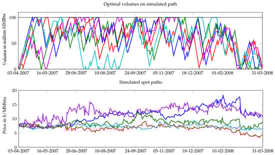
Figure 4.
Valuation of a fast storage unit. For each simulated path (bottom panel), we display (top panel) the storage level corresponding to the optimal policy. Because of the fast injection/withdrawal speed, the storage level reacts quickly to changing market conditions.
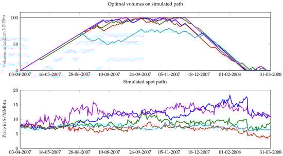
Figure 5.
Valuation of a slow storage unit. For each simulated path (bottom panel), we display (top panel) the storage level corresponding to the optimal policy. Because of the slow injection/withdrawal rate, there is only one storage cycle per year, and the storage value is essentially function of the summer-winter spread.
Note also that the analysis described above depends on the choice of the model, because the backward and forward phases are executed on the sample paths generated by the model itself. In order to make the comparison less model-dependent, we calculate the cumulative cash flows of the estimated optimal strategy, based on spot and futures historical paths. For this reason, we will consider a series of spot and futures curve data from 2003 to 2012, and split it into periods of one year: the storage lease contracts specified in Table 4 start in April of each year, for a one-year period. We run the optimal strategy obtained in the backward phase (for the corresponding storage duration) on the spot and futures historical paths for the related period.
This constitutes a real case test for the optimal strategy and corroborates the relevance of the spot modeling, since it provides the profit that would have been accumulated by the storage manager in a realized path.
Figure 6 and Figure 7 represent the historical spot path realized during the contract period (for both slow and fast units) from April 2007 to April 2008, and the natural gas volumes resulting from the optimal strategy computed on simulated paths (see Figure 4 and Figure 5 for examples of these simulated paths).
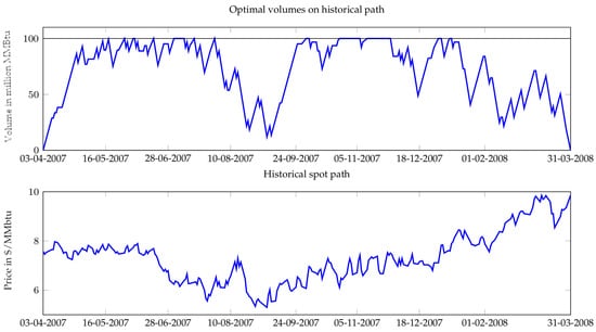
Figure 6.
Historical spot path and optimal volumes (fast storage). bottom panel: historical path, top panel: the optimal storage level on the historical path.
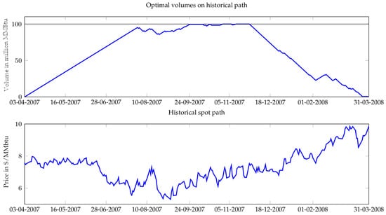
Figure 7.
Historical spot path and optimal volumes (slow storage). bottom panel: historical path, top panel: the optimal storage level on the historical path.
We summarize the results of the valuation algorithm for each period in Table 5 and Table 6, for the fast and slow storage units, when the spot paths are generated according to spot model 2 (19). The tables report, for each period, the intrinsic value (IV) computed according to (3), the estimated extrinsic value (EV) computed by applying the optimal trading strategy (5) to simulated paths, and finally the actual cumulative cash flow obtained by applying the optimal strategy to the actual historical path. The last two columns show the standard deviation of the cumulative cash flows, computed on simulated paths under the optimal strategy.
Table 5.
Fast gas storage valuation (under spot model 2 (19)), in million of US dollars.
Table 6.
Slow gas storage valuation (under spot model 2 (19)), in million of US dollars.
We expect that the extrinsic spot-based strategy will give a larger value than the intrinsic physical futures-based strategy, while our financial hedging strategy is supposed to reduce the uncertainty of gas storage cash flows. For example, the fast storage contract starting in April 2007 has an intrinsic value of while the spot-based strategy gives an extrinsic value of . As expected, the extrinsic strategy allows better financial exploitation of the rights (without obligation) of injection/withdrawal natural gas compared to the conservative intrinsic strategy. In other words, the extrinsic strategy allows better extraction of the optionality of storage. We also note that the hedging strategy yields a significant empirical variance reduction of the cumulative cash flows from to . On the other hand, the intrinsic value of slow storage is equal to , while the spot-based strategy captures a larger optionality value of . Similarly to fast storage, the financial hedging strategy allows an important reduction in variance, from to .
Previous observations about year 2007 remain valid for the other test periods; indeed the extrinsic spot-based strategy always out-performs the intrinsic futures-based strategy, along both simulated and historical paths. The historical back testing over the period 2003–2012 shows that the extrinsic strategy allows for better extraction of storage unit optionality, with a ratio of extrinsic value to intrinsic value as high as for a fast storage unit. This performance of the extrinsic strategy is less significant in the case of slow storage unit, with a ratio up to . This is due to limitations in the deliverability of slow storage. The optimal strategy is not able to fully benefit from gas price volatility, and cannot respond rapidly to favorable price movements. In all cases, hedging with financial instruments provides a significant reduction in the cumulative cash flows uncertainty. The last two columns of Table 5 and Table 6 show a standard deviation reduction factor of up to 10, with better performance for slow storage. This gives the storage manager more insurance to recover a large percentage of the value of the storage contract. Similar conclusions on the advantages of a dynamic hedging with futures are stated by De Jong (2015) in his back tests.
Remark 2.
1. In Section 2.1.2, we presented two heuristic hedging strategies, (8) and (9), based on financial futures contracts. The numerical tests that we have conducted show that the hedging strategy defined by (9) gives better results in the variance reduction of the simulated cash flows under the optimal strategy; in addition, in the historical back testing, (9) yields a better cumulative wealth performance than (8). We emphasize that we have only reported about the better performing hedging strategy (9). 2. We also note that the historical intrinsic value of the gas storage attains a peak in 2006, and shows a clear decline afterwards. This can be intuitively explained by observing the futures curve samples in Figure 1: in 2006, the seasonal spreads were very pronounced, but have been shrinking steadily ever since.
We conclude from the numerical results presented above that the joint modeling of the natural gas spot price and futures curve is a pertinent framework for the gas storage valuation and hedging problem. It allows the unit manager to better exploit storage optionality by monetizing the spot price volatility and seasonality. Indeed, the historical back testing shows that the extrinsic value under this modeling always outperforms the classical intrinsic value, even in the case of slow storage. A joint model for the futures curve with its own risk factors is a more realistic framework for spot and futures markets, since it takes into account the seasonality of the futures curve and the non-convergence of the futures price to the spot price, an unrealistic hypothesis that is often made in the literature. This also allows for a more relevant hedging strategy based on futures contracts, and better tracking of the extrinsic value of gas storage in real market conditions.
5. Model Risk
As previously mentioned, seasonal spreads have become narrower these last years, which means that the bulk of a gas storage value is extrinsic, and needs to be extracted by trading the spread between the spot price and prompt. It is, therefore, important to look closely into the spot modeling and its effect on storage valuation and hedging. We believe that the uncertainty surrounding storage value is primarily due to the modeling of the spot process, since it is the evolution of the spot process ((17) and (19)) that by and large determine the optimal trading strategy. In turn, the futures model mostly affects the quality of the hedge or variance reduction, not the expected value of the storage unit. At least another author (Bjerksund et al. 2011) reaches a similar conclusion while using the rolling intrinsic valuation method.
The purpose of this section is to quantify these statements in the formal framework of model risk measurement, and the section is divided in two parts: we first compare the performances of the two spot models proposed in Section 3.3, using historical data. We focus on the effect of various modeling hypotheses, and on the sensitivity of the storage estimated value with respect to the model parameters. We next define a model risk measure to quantify these uncertainties, following Cont (2006).
5.1. Spot Modeling
In Section 3.3, we proposed two discrete models for the spot price dynamics. The first model, defined in (17), is a discrete version of a mean-reverting model, with a stochastic mean-reversion level equal to the prompt price. The second model (19), directly captures the spread between the spot and the prompt prices, which is a key variable in the optimal management of a storage unit: one tends to buy and store gas when the spot-prompt spread is negative and withdraw it in the opposite case. Since the seasonality of gas prices has been getting weaker in recent years, the principal source of value for the storage unit is the spot-prompt spread rather than the winter-summer spread, so we expect the second model (19) to give good results in recent years.
We run the valuation procedure explained in Section 4, using the two spot models, over a testing period starting in 2003 till 2012. For each year, we compute the actual performance of each model; in particular, we report in Figure 8 and Figure 9 the cumulative cash flows using the optimal spot strategy for historical spot and futures trajectories.
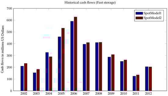
Figure 8.
Historical cash flows for spot models 1 and 2 (fast storage).
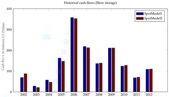
Figure 9.
Historical cash flows for spot models 1 and 2 (slow storage).
In the fast storage case, Figure 8 shows that the spot-prompt spread model (model 2) yields slightly better results than the spot model (model 1) in all but one the test cases (year 2004).
In the slow storage case (Figure 9), the two spot models give comparable results for all periods. In the fast storage case, other tests, not reported in this article, show that spot model 2 yields a lower standard deviation of the cumulative cash flows. This reinforces the observation that spot model 2 is globally better suited for our purpose.
Effect of Spikes Modeling
The presence of spikes in natural gas prices is an essential feature of the dynamics of spot prices. As noted in Section 3.1, these jumps are sudden dislocations between the cash and futures markets due to unexpected imbalances between supply and demand, caused by such factors as unpredicted weather changes, disruptions in the supply chain, or poor anticipations of the global amount of gas in storage.
These spikes can be a source of value for the storage manager, since a large gap between spot and prompt prices can be monetized by buying gas (and selling the corresponding quantity in the futures market) during a negative spike, while doing the opposite trade during a positive spike. Since these are rapidly absorbed by the market, the value can only be captured by fast storage units.
Figure 10 represents the expected cumulative cash flows of a fast storage unit, on simulated paths under spot model (19). All the test periods show that modeling the spikes in the spot dynamics gives a larger extrinsic value for the storage unit, but at the same time it introduces a larger standard deviation for the cumulative cash flows, as illustrated in Figure 11.
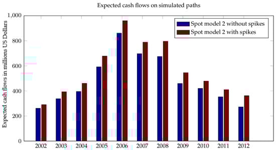
Figure 10.
Expected cash flows on simulated paths.
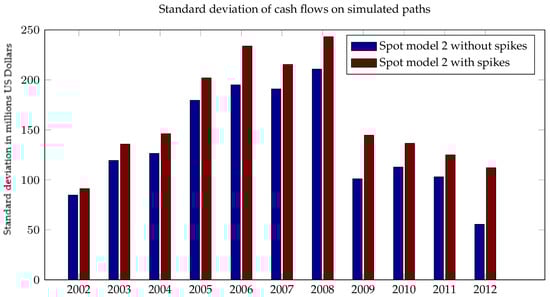
Figure 11.
Standard deviation of cash flows on simulated paths.
A final test of the effect of the spikes modeling is performed on historical spot paths for each test period, and results are shown in Figure 12. The graph shows that modeling the spikes does not make a significant contribution to realized optimal value. This accords with the fact that the models with spikes produce a large standard deviation. In conclusion, and contrary to intuition, this historical back test does not support the need for incorporating spikes in the spot model.
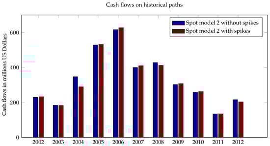
Figure 12.
Cash flows on historical paths.
5.2. Model Risk Measure
In order to quantify the modeling uncertainty, we use the approach introduced by Cont (2006) for measuring the model risk inherent in the pricing of exotic derivative products. The approach may be summarized as follows: Given a set of benchmark quotes for vanilla options (or bid/ask intervals), model uncertainty for an exotic payoff H, is quantified by computing the range of prices of this exotic product, using a set of risk neutral models calibrated to the benchmark vanilla prices, i.e.,
For our gas storage valuation problem, we will adapt this risk measure by using as “calibration” data the historical prices of the futures and spot contracts. The constraint of calibration on vanilla prices is replaced by the success of suitable statistical tests and closeness to the optimal likelihood objective function value of the model.
The family consists of a set of spot models, (17) or (19), which pass the statistical tests imposed by the modeling hypothesis for the noise , which is assumed to be GARCH(1,1). Moreover, the family is restricted to the models that have a likelihood function value close to the optimal one found during the model estimation.
This methodology for the generating the set is broadly similar to the one proposed by Dumont and Lunven (2006), and applied to multi-asset options. In their study, the authors calibrate a multi-assets model to single-asset vanilla options, then build the set by perturbation of the correlation matrix. This yields a family of models that price the benchmark vanilla options perfectly, but differ by their correlation matrix.
In our case, the statistical estimation of the spot model parameters, in (17) or (19), is obtained by classical maximum likelihood methods. The estimation procedure solves:
where is the likelihood function associated with the spot model (17) or (19). This maximization yields an optimal parameters vector , an optimal likelihood function value , and an empirical covariance matrix of the parameter estimates, from which confidence intervals can be computed.
In order to generate the family of spot models, we perturb the optimal parameters by adding a Gaussian noise with the specified covariance matrix to . This yields a set of perturbed parameters , from which we only retain those that satisfy two constraints: first, the inferred GARCH white noise in (18) must pass a statistical test for normality;3 second, the corresponding likelihood function value has to be close to the optimal value : , where is a small constant.
In the following discussion, will be the set , fulfilling the two conditions above. We can now define the associated model risk. The analogue risk measure to (24) can be expressed using (5), with the value function now written to emphasize the dependence of this value function on the parameters . The normalized risk measure is given by:
In this risk measure evaluation, each , is calculated using spot and futures paths simulated under the perturbed model .
Moreover, we propose a second model risk measure based on the performance on realized historical spot and futures paths. For this we define
where represents the cumulative cash flows, computed on the historical path, as defined in (6).
The two risk measures and are computed for each of the test periods from 2003 to 2012, under the two spot models 1 and 2, using a set of 30 perturbed models. The results reported in Table 7 again show a better performance for spot model 2. In fact, this model seems to be less subject to model risk, since it gives a smaller range of prices, compared to spot model 1.
Table 7.
Model risk measure for spot models 1 and 2. All figures are in million $.
One observation that follows clearly from Table 7 is that the range of prices induced by the model uncertainty and measured by and represents a large fraction of the storage value. This shows that the dependence of gas storage valuation on spot modeling is quite significant. While the literature has concentrated its efforts until now on the specification of an optimal valuation strategy, we believe that one should pay more attention to the choice of the spot-futures modeling framework. Referring again to Table 7, model 2 appears to be less sensitive to the change of parameters and is therefore more robust. Fortunately, this is in concordance with the better performance of spot model 2 already observed in Section 5.1. Table 7 shows that the spot-futures valuation framework is subject to a large model risk (average: ). For comparison, the model risk for a basket option has been evaluated to (see Dumont and Lunven (2006)).
6. Conclusions
In this paper we have considered the problem of gas storage valuation and hedging, and specifically investigated the implications of switching from an intrinsic to an extrinsic method of valuation and risk management.
To this end, we have set up an experimental framework which includes a new model for the joint dynamics of the futures curve and the spot price, a back testing engine for pricing storage units and measuring the effectiveness of various hedging strategies, and a method for measuring model risk.
We have then conducted extensive back testing using historical data of futures and spot prices over a period of 10 years.
The numerical tests have confirmed, as expected, that the extrinsic method extracts, on average, more value from the storage units than the traditional intrinsic method.
In order to quantify the stability of our valuation estimates with respect to model uncertainty, we have next defined two model risk measures, inspired by the work of Cont (2006). Our context was however different from Cont’s, in the sense that our models have been estimated on historical data, and not on market data. This motivated a redefinition of the notion of “benchmark data”.
Using those risk measures, we have observed the great sensitivity of gas storage value to modeling assumptions. In fact the model uncertainty, as measured by the size of price range, represents a large proportion of the storage value. This puts into perspective the concentration of effort in the literature on the specification of an optimal valuation strategy. Much more attention should probably be devoted to the discussion of modeling assumptions.
The use of the term extrinsic to qualify the valuation based of stochastic optimization and dynamic hedging should even be questioned. It is borrowed from the theory of financial options, where the extrinsic, or time value of an option can be extracted by owning the option and conducting a self-financed hedging strategy. In our case, the self-funded hedging strategy is the dynamic hedging protocol with futures contract. The parallel stops here however, because this hedging strategy leaves a significant residual risk, and the so-called extrinsic value of storage cannot be safely extracted.
Therefore, the expected discounted cash flow computed by an extrinsic method should not be constructed as a “price”, but as some market index, from which a market price could be derived, probably at a significant discount. Here again, our model risk measurement framework could be of interest, since it provides a distribution of possible values for the storage units.
Acknowledgments
The authors wish to thank the Referees and the Editors for the useful comments which have permitted to improve the first version of the manuscript.
Author Contributions
All the authors have equivalently contributed to the whole paper.
Conflicts of Interest
The authors declare no conflict of interest.
References
- Bjerksund, Petter, Gunnar Stensland, and Frank Vagstad. 2011. Gas storage valuation: Price modelling v. optimization methods. The Energy Journal 32: 203–27. [Google Scholar] [CrossRef]
- Boogert, Alexander, and Cyriel De Jong. 2008. Gas storage valuation using a Monte Carlo method. The Journal of Derivatives 15: 81–98. [Google Scholar] [CrossRef]
- Clewlow, Les, and Chris Strickland. 1999a. A Multi-Factor Model for Energy Derivatives. Working Paper. Sydney: School of Finance and Economics, University of Technology Sydney. [Google Scholar]
- Clewlow, Les, and Chris Strickland. 1999b. Valuing Energy Options in a One Factor Model Fitted to Energy Prices. Sydney: Quantitative Finance Research Group, University of Technology Sydney. [Google Scholar]
- Cont, Rama. 2006. Model uncertainty and its impact on the pricing of derivative instruments. Mathematical Finance 16: 519–47. [Google Scholar] [CrossRef]
- De Jong, Cyriel. 2015. Gas storage valuation and optimization. Journal of Natural Gas Science and Engineering 24 Suppl. C: 365–78. [Google Scholar] [CrossRef]
- Dumont, Philippe, and Christophe Lunven. 2006. Risque de Modèle et Options Multi Sous-Jacents. Rapport de stage, Groupe de Travail ENSAE: Unpublished manuscript. [Google Scholar]
- Eydeland, Alexander, and Krysztof Wolyniec. 2002. Energy and Power Risk Management: New Developments in Modeling, Pricingand Hedging. Hoboken: Wiley. [Google Scholar]
- FERC. 2003. Report of the Natural Gas Price Spike of February 2003; Technical Report; Washington: Federal Energy Regulatory Commission.
- FERC. 2012. State of the Markets, 2011; Technical Report; Washington: Federal Energy Regulatory Commission.
- Gabillon, Jacques. 1991. The Term Structure of Oil Futures Prices. Working Paper, No. M17. Oxford: Oxford Institute of Energy Studies. [Google Scholar]
- Gibson, Rajna, and Eduardo S. Schwartz. 1990. Stochastic convenience yield and the pricing of oil contingent claims. The Journal of Finance 45: 959–76. [Google Scholar] [CrossRef]
- Gray, Josh, and Konstantin Palamarchuk. 2010. Calibration of One and Two-Factor Models for Valuation of Energy Multi-Asset Derivative Contracts. arXiv, arXiv:1011.4547. [Google Scholar]
- Gray, Josh, and Pankaj Khandelwal. 2004. Towards a realistic gas storage model. Commodities Now 7: 1–4. [Google Scholar]
- Hambly, Ben, Sam Howison, and Tino Kluge. 2009. Modelling spikes and pricing swing options in electricity markets. Quantitative Finance 9: 937–49. [Google Scholar] [CrossRef]
- Longstaff, Francis A., and Eduardo S. Schwartz. 2001. Valuing American options by simulation: A simple least-squares approach. Review of Financial Studies 14: 113–47. [Google Scholar] [CrossRef]
- Mastrangelo, Erin. 2007. An Analysis of Price Volatility in Natural Gas Markets; Washington: U.S. Energy Information Administration.
- Nowotarski, Jakub, Jakub Tomczyk, and Rafał Weron. 2013. Robust estimation and forecasting of the long-term seasonal component of electricity spot prices. Energy Economics 39: 13–27. [Google Scholar] [CrossRef]
- Parsons, Cliff. 2013. Quantifying natural gas storage optionality: A two-factor tree model. Journal of Energy Markets 6: 95. [Google Scholar] [CrossRef]
- Safarov, Nemat, and Colin Atkinson. 2017. Natural gas storage valuation and optimization under time-inhomogeneous exponential Lévy processes. International Journal of Computer Mathematics 94: 2147–65. [Google Scholar] [CrossRef][Green Version]
- Schwartz, Eduardo S. 1997. The stochastic behavior of commodity prices: Implications for valuation and hedging. The Journal of Finance 52: 923–73. [Google Scholar] [CrossRef]
- Warin, Xavier. 2012. Gas storage hedging. In Numerical Methods in Finance. Volume 12 of Springer Proceedings in Mathematics, Edited by Chris Rogers. Berlin and Heidelberg: Springer, pp. 421–45. [Google Scholar]
| 1 | We use a 1997–2013 historical data of spot and prompt price, published by the U.S. Energy Information Administration (http://www.eia.gov/dnav/ng/ng_pri_fut_s1_d.htm). |
| 2 | This energy unit can be naturally converted into a volume, under standard conditions for temperature and pressure. |
| 3 | We use a Kolmogorov-Smirnov test for the normality test of the inferred noise z. |


© 2018 by the authors. Licensee MDPI, Basel, Switzerland. This article is an open access article distributed under the terms and conditions of the Creative Commons Attribution (CC BY) license (http://creativecommons.org/licenses/by/4.0/).