Finite Difference Methods for the BSDEs in Finance

Abstract

This paper gives a review of numerical methods for solving the BSDEs, especially, finite difference methods. For numerical methods of finite difference, we should divide them into three branches. Distributed method (or parallel method) should now become a hot topic. It is a key reason we present the review. We give a brief survey on the financial problems. The problems include solution and simulation methods for the BSDEs. We first describe the BSDEs, and then outline the main techniques and main results of the BSDEs. In addition, we compare with the errors between these methods and the Euler method on the BSDEs.

1. Introduction

Primarily motivated by financial problems, backward stochastic differential equations (BSDEs) were developed at high speed during the 1990s. Comparing with Black-Scholes models, Comparing with Black-Scholes models, the BSDEs are more powerful in financial derivative pricing and risk analysis.

To solve many problems in mathematical finance, BSDEs have become powerful mathematical tools. Many problems of option pricing and stochastic optimizations are deal with. For stochastic differential equations (SDEs), BSDEs are terminal value problems. A natural time discretization of the BSDEs works backward in time. Yet, the solution must be adapted to deal with the information. It increases forwards in time, and makes numerical solutions to the BSDEs, become a more challenging problem. Thus, numerical solutions of them have had more and more attention in recent years.

The important class of the BSDEs are the It$\widehat{o}$’s type equations such as

$$d{Y}_t=-f(t,Y_t,Z_t)dt+Z_{t}d{B}_t,Y_T=\xi ,$$

(1)

where $t\in [0,T]$, B is a Brownian motion and $(\xi ,f)$ are given. Here $Z_t$ is a predictable process, f is called the generator or the driver, $Y_T=\xi$ is the terminal condition.

Suppose $(Y,Z)$ is the solution of standard BSDE (1). The equations can be interpreted as a stochastic integral equation of the form

$$Y_t=\xi +{\int }_t^{T}f(s,Y_s,Z_s)ds-{\int }_t^T{Z}_{s}d{B}_s,0\le t\le T,$$

(2)

where B is a Brownian motion and $(\xi ,f)$ are given. Then the solution satisfies,

$$Y_t=Y_{t_0}-{\int }_t^{t_0}f(s,Y_s,Z_s)ds+{\int }_t^{t_0}{Z}_{s}d{B}_s,0\le t,t_0\le T.$$

(3)

We now assume that ($Y^{\pi },Z^{\pi }$) is some adapted approximation of the solution $(Y,Z)$, which is piecewise constant with respect to a partition $\pi =\{t_0,t_1,\cdots ,t_n\}$ of $[0,T]$. Here f depends only on Y.

We now consider the discrete version of the BSDE (1):

$$Y_{t_i}^{\pi }={\xi }^{\pi }+\frac{1}{n}\sum _{j=i}^{n}f(Y_{t_j}^{\pi })-\sum _{j=i}^n{Z}_{t_j}^{\pi }(B_{t_{j+1}}^{\pi }-B_{t_j}^{\pi }).$$

(4)

It has a unique solution $(Y_t^{\pi },Z_t^{\pi })$ due to the martingale $B^{\pi }$.

1.1. BSDEs via Financial Problems

The BSDEs are widely used in many financial problems. Due to the structure of option pricing problems, it allows to be solved by numerical methods. In the same time, we can have confidence intervals, lower and upper bias of numerical solutions. For general nonlinear BSDEs, a similar way, to construct lower and upper approximations, is not available. Nonetheless, the intricate interplay, between the time discretization and the design of the estimation, persists for nonlinear BSDEs in a similar way as for the option problems.

In a complete market, contingent claim valuation theory can be expressed through BSDEs. The price process Y is a solution of the BSDE. For the usual valuation with payoff $\xi =\mathsf{\Phi }\left(X\right)$, Y is the replicating portfolio value, and Z is the related hedging strategy. Here the driver f is linear with regard to Y and Z.

In incomplete markets, the F$\ddot{o}$llmer-Schweizer method is solving a BSDE. For trading constraints, the super-replication price is the limit of the BSDEs. Peng introduced g-expectation (here g is the driver) as a nonlinear pricing rule, and showed the connection between the BSDEs and risk measures, ${\epsilon }_t$ is related to a BSDE about $Y_t$.

The BSDEs appear in many financial problems, for example, the pricing and the hedging of some options. These options include call option, put option, Europe option, American option, lookback options, digital options and compound option, among others. The problems have indifference pricing (Rouge and El Karoui 2000), recursive utility (El Karoui et al. 1997), robust optimization (Peng and Wu 1999), among others. In addition, through the BSDEs, portfolio selection, risk control and hedging are obtained.

Here, we give some examples of terminal conditions $\xi =\mathsf{\Phi }\left(X\right)$. A large class of exotic payoffs satisfies a functional Lipschitz condition, for example, vanilla payoff is $\mathsf{\Phi }\left(X\right)=\varphi \left(X_T\right)$; asian payoff is $\mathsf{\Phi }\left(X\right)=\varphi (X_T,{\int }_0^T{X}_{t}dt)$; lookback payoff is $\mathsf{\Phi }\left(X\right)=\varphi (X_T,{min}_{t\in [0,T]}{X}_t,{max}_{t\in [0,T]}{X}_t)$. Then we can say that the BSDEs are now inevitable tools in mathematical finance.

1.2. Branches of Finite Difference Methods for the BSDEs

To solve the financial problems by numerical approximation in time, one can resort to either finite difference (FD) methods, or more general finite element (FE) methods, or even finite volume (FV) methods. We also note that, there is in fact, no absolute border between these methods. In a sense, Monte Carlo (MC) methods are special cases of binomial methods (namely, tree methods). A complete scheme in scientific computation is below:

FV methods ⊃ FE methods ⊃ FD methods ⊃ Tree methods ⊃ MC methods.

FD, FE and FV have their good points: The theory of FD is mature and the precision of it is optional. The advantage of FD is easy to program and parallel. FE is hard to handle a large amount of computation. Parallelism is not as intuitive as FD and FV. FE parallelism, however, is a good direction for current and future applications. FV can be applied to irregular grids and is suitable for parallel. But the precision of it is basically only two order.

The steps of the FD methods include discretizing the localized time-space domain; choosing suitable discrete model; solving the discrete model system, among others.

The most elementary ones are the FD methods for the BSDEs. Up to now basically, three branches of the FD methods have been considered. The main branch of the methods is the FD solution of a related parabolic PDE for the given BSDE. Based on the Ma et al. (1994) method, the FD methods for the BSDEs have been intruduced by (Douglas et al. 1996; Milstein and Tretyakov 2006), among others. Here the solution problem roughly reduces to the approximation of a quasi-linear parabolic Cauchy problem. This approach relies on some smoothness assumptions on the coefficients of the BSDEs, and the spatial dimensions of the PDEs.

A second branch of the methods works backward in time, and deals with the stochastic problem directly. Chevance (1997) used a random time discretization for it. The work of Ma et al. (2002) belongs to this class, however, replacing, the Brownian motion in the approximative equation. This kind of work can also be seen in Zhang (2004); Bouchard and Touzi (2004); Gobet et al. (2005); Gobet and Labart (2007); Gobet and Labart (2010); Gobet et al. (2016), among others.

A third branch of the methods represents the calibration methods. To improve the efficiency of given methods, some researchers developed parallel and distributed methods, variance reduction methods. For example, Peng et al. (2010) developed a parallel method of reflected BSDEs on option pricing. It is a method with block allocation. Tran (2011) reconstructed the four step method with some new conditions in FBSDEs, which is associated with Schwarz waveform relaxation method, to parallelize the related equations. Bender and Moseler (2010) introduced importance sampling to MC methods for pricing problems, represented by the BSDEs.

In addition, the following FD methods are especial interest: the Malliavin calculus approach (Bouchard and Touzi 2004; Bouchard and Elie 2008), the linear regression method or the Longsta-Schwartz method (Lemor et al. 2006), the Picard iteration method (Bender and Denk 2007), the quantization method (Bally and Pages 2002; Bally and Pages 2003), among others. These methods work well in the setting of high dimensions. There are also many works in numerical methods for non-Markovian BSDEs. For example, Ma et al. (2002).

1.3. Recent Development of Some New BSDEs

In this century, the theories about the BSDEs are more and more mature. Yet, there are still plenty of the research areas that appeal to many researchers. For example, the solution problems are very popular among researchers in finance. Rouge and El Karoui (2000) introduced a class of the BSDEs. They solved the utility maximization problems in an incomplete market. Kobylanski (2000) solved a type of the BSDEs with drivers, which are the quadratic growths of Z. On top of that, there are a kind of new developed BSDEs such that second-order BSDEs, time-delayed BSDEs, finite-horizon BSDEs, quadratic BSDEs, anticipated BSDEs (Peng and Yang 2009), BSDEs with a Lipschitz condition, BSDEs with Markov chains, among others.

The rest of the paper is organized as follows. In Section 2, we describe the solution methods of some related BSDEs, give some analysis for them. In Section 3, we state the solution methods of the FBSDEs. Parallel methods are discussed in Section 4, while Section 5 gives discussion and conclusion.

2. FD Solutions of Some Related BSDEs in Finance

A relevant problem in the BSDEs is to propose the FD methods to approximate the solution of them. Several efforts have been given as well. For example, Chevance (1997) proposed a general method for the BSDEs. Zhang (2004) proposed a method for a class of the BSDEs, with related terminal values. Peng and Xu (2008) studied some different methods for the BSDEs, based on random walk framework. They introduced the implicit and explicit methods in BSDEs and reflected BSDEs. To get an FD solution of the BSDEs, researchers suppose time-discretization.

2.1. FD Solutions of the BSDEs with Reflections in Finance

In the subsection, we are interested in the FD solutions of the BSDEs with Reflections (BSDERs). For researching the BSDERs, one of the main motivations is solving the hedging problem for American options. The BSDERs have the following forms,

$$\begin{array}{cc}\hfill Y_t& =\xi +{\int }_t^{T}f(s,Y_s,Z_s)ds-{\int }_t^T{Z}_{s}d{B}_s+K_T-K_t,0\le t\le T,\hfill \\ \hfill Y_t& \ge L_t,0\le t\le T,\mathrm{and}{\int }_0^T(Y_t-L_t)d{K}_t=0.\hfill \end{array}$$

(5)

where $L_t=L_0+{\int }_0^t{l}_{s}ds+{\int }_0^t{\sigma }_{s}d{B}_s,0\le t\le T$, $\xi =\mathsf{\Phi }({\left(B_s\right)}_{\{0\le s\le T\}})$, $K_t$ is continuous and increasing, $l_t$ is a smooth function, and $K_0=0$.

Now we discuss some applications of the BSDERs, for example, optimal stopping problem (American option). In an American call option, the wealth process $Y_t$ satisfies the following BSDERs,

$$\begin{array}{cc}\hfill X_t& =X_0+{\int }_0^t\mu X_{s}ds+{\int }_0^t\sigma X_{s}dBs,0\le t\le 1,\hfill \\ \hfill Y_t& ={(X_T-K)}^{+}-{\int }_t^T[r{Y}_s+(\mu -r)Z_s]ds-{\int }_t^T\sigma Z_{s}dBs,\hfill \end{array}$$

(6)

and $Y_t\ge {(X_t-K)}^{+}$, $0\le t\le inf\{t,Y_t-{(X_t-K)}^{+}\}$. Here $\sigma$ is volatility rate, r is uniformly bounded, K is a constant.

The BSDERs apply to American put option in the following case:

$$Y_T=\xi ={(K-X_T)}^{+}.$$

For option pricing with differential interest rates, $(\mu -r)$ is related to $Y_t$ and $Z_t$ in Equation (6).

We assume that $X=\{X_t,0\le t\le T\}$ is the risk asset, r is constant. Under some assumptions, the equation is given through a reflected BSDE, together with the forward equation of X. We then can have $Y_0$, the option value.

There are some FD methods for solving the BSDERs, including max method, penalization method, regularization method and the forth. We will approximate the solution of the BSDERs. On small interval $[i\delta ,(i+1\left)\delta \right]$, Equation (5) can be approximated through the following discrete equation,

$$\begin{array}{cc}\hfill Y_{t_i}^{\pi }& =Y_{t_{j+1}}^{\pi }+f(t_i,Y_{t_i}^{\pi },Z_{t_i}^{\pi })\delta +K_{t_{i+1}}-K_{t_i}-Z_{t_i}^{\pi }{\epsilon }_{j+1}^{\pi }\sqrt{\delta }\hfill \\ \hfill Y_{t_i}^{\pi }& \ge L_{t_i}^{\pi },(Y_{t_i}^{\pi }-L_{t_i}^{\pi })(K_{t_{i+1}}-K_{t_i})=0,\hfill \end{array}$$

(7)

here

$$L_{t_i}^{\pi }=L_0+\delta {\mathsf{\Sigma }}_{j=0}^{i-1}{l}_{t_j}+{\mathsf{\Sigma }}_{j=0}^{i-1}{\sigma }_{t_j}{\epsilon }_{j+1}^{\pi }\sqrt{\delta }.$$

Equation (7) is a discrete BSDER, with terminal condition ${\xi }^{\pi }=\mathsf{\Phi }({\mathsf{\Sigma }}_{j=1}^i{\epsilon }_{j+1}^{\pi }\sqrt{\delta })$. In the case $f=0$, $\xi =\varphi \left(X_1\right)$ and $L=\varphi$, Y is the Snell envelope of $\varphi \left(X\right)$, related to the super-hedging price with payoff $\varphi$.

An important method is penalization method for the equations. For $p\in N$, the penalization equation is

$$Y_t^p=\xi +{\int }_t^{T}f(s,Y_s^p,Z_s^p)ds+p{\int }_t^T{(Y_s^p-L_s)}^{-}ds-{\int }_t^T{Z}_s^{p}d{B}_s.$$

(8)

The solution of the BSDERs can be approximated by the solution of Equation (8). We have the following discrete penalized BSDEs on the small interval $[i\delta ,(i+1\left)\delta \right]$,

$$Y_{t_i}^{p,\pi }=Y_{t_{j+1}}^{p,\pi }+f(t_i,Y_{t_i}^{p,\pi },Z_{t_i}^{p,\pi })\delta +p{(Y_{t_i}^{p,\pi }-L_{t_i}^{\pi })}^{-}\delta -Z_{t_i}^{p,\pi }{\epsilon }_{j+1}^{\pi }\sqrt{\delta }.$$

(9)

If $\mathsf{\Gamma }$ is a close subset in $\mathbb{R}$. Let $d_{\mathsf{\Gamma }}(Y,Z)={inf}_{(Y^{\prime },Z^{\prime })\in \mathsf{\Gamma }}\left\{\right|Y-Y^{\prime }|+|Z-Z^{\prime }\left|\right\}$, $(Y_t,Z_t)\in {\mathsf{\Gamma }}_t$ in Equation (8). After the same discretization for the BSDEs, for each positive number p, we get the following discrete equation on $[i\delta ,(i+1\left)\delta \right]$,

$$Y_{t_i}^{p,\pi }=Y_{t_{j+1}}^{p,\pi }+f(t_i,Y_{t_i}^{p,\pi },Z_{t_i}^{p,\pi })\delta +p{d}_T\delta -Z_{t_i}^{p,\pi }{\epsilon }_{j+1}^{\pi }\sqrt{\delta },$$

(10)

with the discrete terminal condition $Y_T^{\pi }={\xi }^{\pi }$.

Now we consider $d_T(Y,Z)={(Y-\varphi \left(Z\right))}^{-}\ge 0$. For some p large enough, We have the following discrete equation about the small interval $[i\delta ,(i+1\left)\delta \right],0\le i\le n-i$

$$Y_{t_i}^{p,\pi }=Y_{t_{j+1}}^{p,\pi }+f(t_i,Y_{t_i}^{p,\pi },Z_{t_i}^{p,\pi })\delta +p{(\varphi \left(Z_{t_i}^{p,\pi }\right)-Y_{t_i}^{p,\pi })}^{+}\delta -Z_{t_i}^{p,\pi }{\epsilon }_{j+1}^{\pi }\sqrt{\delta }.$$

(11)

We use the solution approximation of $(Y,Z,K)$, for the following BSDER,

$$\begin{array}{cc}\hfill Y_t& =\varphi \left(X_1\right)+{\int }_t^{1}f(s,Y_s,Z_s)ds-{\int }_t^1{Z}_{s}d{B}_s+K_1-K_t,0\le t\le 1,\hfill \\ \hfill Y_t& \ge L_t,0\le t\le 1,\mathrm{and}{\int }_0^1(Y_t-L_t)d{K}_t=0.\hfill \end{array}$$

(12)

where $L=\left\{L_t\right\}$ is the reflecting barrier, $K_t$ is continuous and increasing, $K_0=0$. That is for Equation (5) while $T=1$.

For Equation (12), this approximation get a backward Euler scheme $(Y_{t_i}^{\pi },{\tilde{Z}}_{t_i}^{\pi })$ for the following form,

$$\begin{array}{cc}\hfill {\tilde{Z}}_{t_i}^{\pi }& ={(t_{i+1}-t_i)}^{-1}E[Y_{t_{i+1}}^{\pi }(B_{t_{i+1}}-B_{t_i})|{\mathcal{F}}_{t_i}];\hfill \\ \hfill {\tilde{Y}}_{t_i}^{\pi }& =E(Y_{t_i+1}^{\pi }|{\mathcal{F}}_{t_i})+f(X_{t_i}^{\pi },{\tilde{Y}}_{t_i}^{\pi },{\tilde{Z}}_{t_i}^{\pi })(t_{i+1}-t_i);\hfill \\ \hfill Y_{t_i}^{\pi }& =\mathcal{R}(t_i,X_{t_i}^{\pi },{\tilde{Y}}_{t_i}^{\pi }),i\le n-1,\hfill \end{array}$$

(13)

with $Y_T^{\pi }=g\left(X_T^{\pi }\right)$. Here $X^{\pi }$ is the Euler method, associated to X,

$$\mathcal{R}(t,X,Y)=Y+{[L\left(X\right)-Y]}^{+}{\mathbf{1}}_{t\in \mathfrak{R}\setminus \{0,T\}},$$

for a partition $\mathfrak{R}=\{0=r_0<r_1<\cdots <r_k=1\}\supset \pi$. ${\mathcal{F}}_t$ is the completed filtration of $B_t$.

Given an approximation ${\widehat{E}}_i^{\pi }$ of $E[·|{\mathcal{F}}_{t_i}]$, we then have the following backward method,

$$\begin{array}{cc}\hfill {\tilde{Z}}_{t_i}^{\pi }& ={(t_{i+1}-t_i)}^{-1}{\widehat{E}}_i^{\pi }[Y_{t_{i+1}}^{\pi }(B_{t_{i+1}}-B_{t_i})],\hfill \\ \hfill {\tilde{Y}}_{t_i}^{\pi }& ={\widehat{E}}_i^{\pi }(Y_{t_i+1}^{\pi }|{\mathcal{F}}_{t_i})+f(X_{t_i}^{\pi },{\tilde{Y}}_{t_i}^{\pi },{\tilde{Z}}_{t_i}^{\pi })(t_{i+1}-t_i),\hfill \end{array}$$

with $Y_T^{\pi }=g\left(X_T^{\pi }\right)$.

The FD procedures, for such methods, have been introduced in Bally and Pages (2002). For more general analysis, Ma and Zhang (2005) obtained a related bound. They gave the following representation of Z:

$$Z_t=E[\varphi \left(X_1\right)N_1^t+{\int }_t^{1}f(X_s,Y_s,Z_s)N_s^{t}ds+{\int }_t^1{N}_s^{t}d{K}_s|{\mathcal{F}}_t]\sigma \left(X_t\right)$$

(14)

where

$$N_1^t=\frac{1}{1-t}{\int }_t^1\sigma {\left(X_s\right)}^{-1}\mathsf{\nabla }{X}_{s}d{B}_s{(\mathsf{\nabla }{X}_t)}^{-1}.$$

here $\mathsf{\nabla }X$ is the variation process of X.

$$Y_t^{\pi }=\varphi \left(X_1\right)+{\int }_t^{1}f(X,Y^{\pi },Z^{\pi })ds-{\int }_t^1{Z}_s^{\pi }d{B}_s+K_1^{\pi }-K_t^{\pi }$$

(15)

where $K_t^{\pi }={\mathsf{\Sigma }}_{j=1}^{k-1}{[f\left(X_{s_j}\right)-Y_{s_j}^{\pi }]}^{+}{\mathbf{1}}_{s_j\le t}$.

$$Z_t^{\pi }=E[\varphi \left(X_1\right)N_1^t+{\int }_t^{1}f(X,Y^{\pi },Z^{\pi })N_s^{t}ds+\sum _{k=0}^k{N}_{s_k}^t\mathsf{\Delta }{K}_{s_k}^{\pi }{\mathbf{1}}_{t<s_k}|{\mathcal{F}}_t]\sigma \left(X_t\right)$$

for $t\in [s_j,s_{j+1})$, where $\mathsf{\Delta }{K}_{s_k}^{\pi }={[f\left(X_{s_k}\right)-Y_{s_k}^{\pi }]}^{+}$.

Bouchard and Chassagneux (2008) gave another regularity analysis. The main advantage is providing a representation of $Z^{\pi }$, through the next reflection time:

$$\begin{array}{cc}\hfill Z_t^{\pi }& =E[D\varphi \left(X_1\right){\eta }_1^{\pi }{\mathbf{1}}_{{\tau }_j=1}+DL\left(X_{{\tau }_j}\right){\eta }_{{\tau }_j}^{\pi }{\mathbf{1}}_{{\tau }_j=<1}\hfill \\ \hfill & +{\int }_t^{{\tau }_j}{D}_{s}f(X,Y^{\pi },Z^{\pi }){\eta }_r^{\pi }{d}_r\left|{\mathcal{F}}_t\right]{\left({\eta }_t^{\pi }\right)}^{-1}\sigma \left(X_t\right),\hfill \end{array}$$

(16)

for $t\in [s_j,s_{j+1})$, where ${\tau }_j=inf\{s\in \mathfrak{R}|s\ge s_{j+1},L\left(X_s\right)>Y_s^{\pi }\}\wedge 1$ and ${\eta }^{\pi }$ is a function of with $(X,Y^{\pi },Z^{\pi })$ in place of $(X,Y,Z)$. Here $(D\varphi ,DL,Df)$ are the Malliavin derivatives.

These above methods are implicit methods, based on random walk, with one continuous lower barrier. These methods are the discrete-time approximations. The equations are related to stochastic stopping games, game options. Let $K_t=K_t^{+}-K_t^{-}$ in Equation (5), the equations are called the BSDEs with doubly reflections. They are corresponding to the stochastic stopping games, see also Chassagneux (2009).

2.2. FD Solutions of the BSDEs with Jumps

The BSDEs with jumps (BSDEJs), introduced by Situ (1997), Situ and Yin (2003), Royer (2006), and Zhu (2010), are as follows:

$$Y_t=\xi +{\int }_t^{T}f(s,Y_s,Z_s,U_s)ds-{\int }_t^T{Z}_{s}d{B}_s-{\int }_{(t,T]\times \mathbb{R}}{U}_s\left(x\right)\tilde{N}(ds,dx),$$

(17)

where $0\le t\le T$, $\tilde{N}(ds,dx)=N(ds,dx)-\nu (ds,dx)$ is a compensated measure in $[0,T]\times \mathbb{R}$. U is the jump component. The BSDEJs are used to the evaluation of financial derivatives.

With $|\pi |={max}_i|t_{i+1}-t_i|$, the partition $\pi$ is given on of $[0,T]$, $X^{\pi }$ is a corresponding discretization of X, and $Y_T^{\pi }=\xi$. The backward Euler method $(Y^{\pi },Z^{\pi },U^{\pi })$ for $(Y,Z,U)$, is the following implicit method,

$$\begin{array}{cc}\hfill Y_{t_i}^{\pi }& =Y_{t_{i+1}}^{\pi }+f(t_i,Y_{t_{i+1}}^{\pi },Z_{t_i}^{\pi },U_{t_i}^{\pi })\tilde{N}((t_i,t_{i+1}]\times \mathbb{R}),\hfill \\ \hfill Z_{t_i}^{\pi }& =\frac{1}{(t_{i+1}-t_i)}{Y}_{t_{i+1}}^{\pi }(B_{t_{i+1}}-B_{t_i}),\hfill \\ \hfill U_{t_i}^{\pi }& =\frac{1}{(t_{i+1}-t_i)}{Y}_{t_{i+1}}^{\pi }\tilde{N}((t_i,t_{i+1}]\times \mathbb{R}),0\le i\le n-1,\hfill \end{array}$$

(18)

Here the symbols are the same as the above equations.

Similarly, for the BSDEJs, we can also use max method, penalization method, regularization method and so on.

The reflected BSDEs can be considered as the extensions of BSDEs with jumps. They are with jumps see, (Essaky 2008) and constrained BSDEs with jumps see, (Elie and Kharroubi 2010; Kharroubi et al. 2010).

2.3. FD Solutions of Second Order BSDEs

We now give the following second order BSDEs (2BSDEs):

$$\begin{array}{cc}\hfill d{X}_t& =\sigma \left(X_t\right)d{B}_t\hfill \\ \hfill d{Y}_t& =-f(t,X_t,Y_t,Z_t,{\mathsf{\Gamma }}_t)dt+Z\sigma \left(X_t\right)d{B}_t\hfill \\ \hfill d{Z}_t& ={\alpha }_{t}dt+{\mathsf{\Gamma }}_t\sigma \left(X_t\right)d{B}_t,0\le t\le T,\hfill \end{array}$$

(19)

with $Y_T=\varphi \left(X_T\right)$. Here $\alpha ,\mathsf{\Gamma },\sigma ,\varphi$ and f are deterministic functions.

With $\left|\pi \right|={max}_i|t_{i+1}-t_i|$, the partition $\pi$ of $[0,T]$ is given and a corresponding discretization $X^{\pi }$ of X, $Y_T^{\pi }=g\left(X_T^{\pi }\right)$. The Euler method is as following,

$$\begin{array}{cc}\hfill Y_{t_i}^{\pi }& =E_i^{\pi }[Y_{t_{i+1}}^{\pi }]+f(t_i,X_{t_i}^{\pi },Y_{t_i}^{\pi },Z_{t_i}^{\pi },{\mathsf{\Gamma }}_{t_i}^{\pi })(t_{i+1}-t_i),\hfill \\ \hfill Z_{t_i}^{\pi }& =\frac{\sigma {\left(X_{t_i}^{\pi }\right)}^{-1}}{(t_{i+1}-t_i)}{E}_i^{\pi }[Y_{t_{i+1}}^{\pi }(B_{t_{i+1}}-B_{t_i})],\hfill \\ \hfill {\mathsf{\Gamma }}_{t_i}^{\pi }& =\frac{\sigma {\left(X_{t_i}^{\pi }\right)}^{-1}}{(t_{i+1}-t_i)}{E}_i^{\pi }[Z_{t_{i+1}}^{\pi }(B_{t_{i+1}}-B_{t_i})],0\le i\le n-1.\hfill \end{array}$$

(20)

Cheridito et al. (2007) investigated the 2BSDEs in Markovian framework. A solution of the 2BSDEs is a process $(Y,Z,\alpha ,\mathsf{\Gamma })$. They supposed a solution with $Y_t=V(t,X_t)$. They considered the fully nonlinear PDE (with $\mathcal{L}V=\frac{1}{2}Tr[\sigma {\sigma }^T{D}^{2}V]$)

$$\frac{\partial V}{\partial t}+\mathcal{L}v(t,x)+f(t,x,v(t,x),Dv(t,x),D^{2}v(t,x))=0$$

with $v(T,x)=\varphi \left(x\right)$.

If the above equation has a smooth solution, then

$${\widehat{Y}}_t=v(t,X_t),{\widehat{Z}}_t=Dv(t,X_t),{\widehat{\alpha }}_t=\mathcal{L}Dv(t,X_t),{\widehat{\mathsf{\Gamma }}}_t=V_{xx}(t,X_t),$$

is a solution of the 2BSDEs.

3. FD Solutions of the FBSDEs in Finance

In this section we survey the novel solution development of some FBSDEs in finance. An FBSDE is a BSDE where the randomness in the driver, comes from some underlying forward process. The FBSDEs have numerous applications in finance problems. The main property is that, the FD solution can be given by functions of time and state process. For the FBSDEs, several approximation methods were proposed. The first one was from four-step method, by Douglas et al. (1996). There are many methods proposed, foe example, Markov chain approximation (Ma et al. 2002), regression methods (Gobet et al. 2005), quantization methods (Bally and Pages 2002; Bally and Pages 2003), the MC Malliavin method (Bouchard and Touzi 2004). Makarov (2003) and Milstein and Tretyakov (2006) also proposed some difference methods for the FBSDEs. Delarue and Menozzi (2006) proposed a probabilistic method. These methods need to discretize the regular grid space, and are not proposed in high-dimensional setting. We now discuss are related to difference solutions of coupled FBSDEs and decoupled FBSDEs in finance.

Consider a coupled FBSDE of the following form,

$$\begin{array}{cc}\hfill dX& =b(t,X,Y,Z)dt+\sigma (t,X,Y,Z)d{B}_t,X\left(t_0\right)=x;\hfill \\ \hfill dY& =\varphi (t,X,Y)dt-f(t,X,Y,Z)dt+Zd{B}_t,Y_T=\varphi \left(X_T\right),\hfill \end{array}$$

(21)

where $b,\sigma ,\varphi$ and f are deterministic functions.

We consider the following representation formula of the coupled FBSDEs:

$$\begin{array}{cc}\hfill X_t& =x+{\int }_0^{t}b(s,X_s,Y_s,Z_s)ds+{\int }_0^t\sigma (s,X_s,Y_s,Z_s)dBs;\hfill \\ \hfill Y_t& =\varphi \left(X_T\right)+{\int }_t^{T}f(s,X_s,Y_s,Z_s)ds-{\int }_t^T{Z}_{s}d{B}_s,\hfill \end{array}$$

(22)

with $Y_T=\varphi \left(X_T\right)$, $B_t$ is on $[0,T]$. The solution consists of a triplet $(X,Y,Z)$, i.e., the forward part, the backward part and the control part.

3.1. Markovian Iteration of Coupled FBSDEs

A time discretization of Equation (22) is

$$\begin{array}{cc}\hfill X_{t_{i+1}}^{\pi }& =X_{t_i}^{\pi }+b(t_i,X_{t_i}^{\pi },Y_{t_i}^{\pi })h+\sigma (t_i,X_{t_i}^{\pi },Y_{t_i}^{\pi })(B_{t_{i+1}}-B_{t_i}),\hfill \\ \hfill Z_{t_i}^{\pi }& =\frac{1}{h}{E}_{t_i}[Y_{t_{i+1}}^{\pi }(B_{t_{i+1}}-B_{t_i})],\hfill \\ \hfill Y_{t_i}^{\pi }& =E_{t_i}[Y_{t_{i+1}}^{\pi }+f(t_i,X_{t_i}^{\pi },Y_{t_{i+1}}^{\pi },Z_{t_i}^{\pi })h];i=1,\cdots ,n,\hfill \end{array}$$

(23)

where $h=T/n$ and $t_i=ih$. Here $E_{t_i}$ denotes the conditional expectation $E\{·|{\mathcal{F}}_{t_i}\}$, $X_0^{\pi }=x,Y_T^{\pi }=\varphi \left(X_T^{\pi }\right).$

Bender and Zhang (2008) combined the above time discretization about an iterative method, and introduced Markovian iteration for coupled FBSDEs, which reads, $u_i^{\pi ,0}\left(x\right)=0$, $X_0^{m,\pi }=x,Y_T^{m,\pi }=g\left(X_T^{m,\pi }\right)$ and

$$\begin{array}{cc}\hfill X_{t_{i+1}}^{m,\pi }& =X_{t_i}^{m,\pi }+b(t_i,X_{t_i}^{m,\pi },u_i^{m-1,\pi }\left(X_{t_i}^{m,\pi }\right))h\hfill \\ \hfill & +\sigma (t_i,X_{t_i}^{m,\pi },u_i^{m-1,\pi }\left(X_{t_i}^{m,\pi }\right))(B_{t_{i+1}}-B_{t_i}),\hfill \\ \hfill Z_{t_i}^{m,\pi }& =\frac{1}{h}{E}_{t_i}[Y_{t_{i+1}}^{m,\pi }(B_{t_{i+1}}-B_{t_i})],\hfill \\ \hfill Y_{t_i}^{m,\pi }& =E_{t_i}[Y_{t_{i+1}}^{m,\pi }+f(t_i,X_{t_i}^{m,\pi },Y_{t_{i+1}}^{m,\pi },Z_{t_i}^{m,\pi })h],\hfill \\ \hfill u_i^{m,\pi }& (X_{t_i}^{m,\pi })=Y_{t_i}^{m,\pi }.\hfill \end{array}$$

(24)

The main advantage is that $Y_{t_i}^{m,\pi }$ is a function of time t and $X_{t_i}^{m,\pi }$, but does not depend on $\{X_{t_i}^{\mu ,\pi },\mu =1,\cdots ,m-1\}$.

The MC efficiency is increased through variance reduction. Bender and Moseler (2010) introduced importance sampling for pricing problems on the FBSDEs. Importance sampling change the drift through a measure change. In addition, Antonelli and Pascucci (2002) concern some financial application of FBSEs.

3.2. Four-Step Method for Solving Coupled FBSDEs

Due to the four-step scheme, the solution of (22) is connected with the following semilinear PDE:

$$\begin{array}{c}\frac{\partial u}{\partial t}+\sum _{i=1}^d{a}^i(t,x,u)\frac{\partial u}{\partial x^i}+\frac{1}{2}\sum _{i,j=1}^d{a}^{ij}(t,x,u)\frac{{\partial }^{2}u}{\partial x^i\partial x^j}\hfill \\ =\varphi (t,x,u)-\sum _{k=1}^n{f}^k(t,x,u)\sum _{i=1}^d{\sigma }^{ik}(t,x,u)\frac{\partial u}{\partial x^i},0\le t\le T,\hfill \end{array}$$

(25)

where

$$a^{ij}=\sum _{i=1}^d{\sigma }^{ik}{\sigma }^{jk},u(T,x)=\varphi \left(x\right).$$

Assume that the solution $u(t,x)$ of Equation (23) is known. Consider the following equation:

$$\begin{array}{cc}\hfill X_t& =x+{\int }_0^{t}b(s,X_s,u(s,X_s))ds+{\int }_0^t\sigma (s,X_s,u(s,X_s))dBs,\hfill \\ \hfill Y_t& =u(t,X_t),\hfill \\ \hfill Z_t^j& =\sum _{i=1}^d{\sigma }^{ij}(t,X_t,Y_t)\frac{\partial u}{\partial x^i}(t,X_t),j=1,\cdots ,n.\hfill \end{array}$$

(26)

Defined by Equation (24), $(X_t,Y_t,Z_t)$ would give an adapted solution of the FBSDE on Equation (22).

In addition, Ma et al. (2008) obtained the unique adapted solution of (22) through the following steps:

Step 1.

We define Z such that

$$Z(t,X_t,Y_t,p)=p\sigma (t,X_t,Y_t).$$

Step 2.

We use $Z(t,X_t,Y_t,p)$ instead of $\sigma (t,X_t,Y_t)$, solve Equation (23).

Step 3.

Through $u(t,X_t)$ and $Z(t,X_t,Y_t,p)$, we solve the forward SDE:

$$X_t=x+{\int }_0^{t}b(s,X_s,u(s,X_s),Z(s,X_s,u(s,X_s),\frac{\partial u}{\partial x}))ds+{\int }_0^t\sigma (s,X_s,u(s,X_s))dBs.$$

Step 4.

Set

$$Y_t=u(t,X_t),Z_t^j=\sum _{i=1}^d{\sigma }^{ij}(t,X_t,Y_t)\frac{\partial u}{\partial x^i}(t,X_t),j=1,\cdots ,n.$$

Delarue and Menozzi (2006) exploited the relation to quasilinear parabolic PDEs via Ma-Protter-Yong method. $(X,Y,Z)$ are given by

$$Y_t=u(t,X_t),Z_t=u_x(t,X_t)\sigma (t,X_t,u(t,X_t)),$$

(27)

where u is a classical solution of the following quasilinear PDE,

$$\frac{\partial }{\partial t}u(t,x)+b(t,x,u(t,x))\frac{\partial }{\partial x}u(t,x)+\frac{1}{2}trace(\sigma {\sigma }^T(t,x,u(t,x))\frac{{\partial }^2}{\partial x^2}u(t,x)+f(t,x,u(t,x))=0,$$

(28)

with $u(T,x)=\varphi \left(x\right)$.

3.3. Layer Method of Decoupled FBSDEs

We consider the difference solution of the following decoupled FBSDE:

$$\begin{array}{cc}\hfill X_t& =X_0+{\int }_0^{t}b(s,X_s)ds+{\int }_t^T\sigma (s,X_s)d{B}_s,0\le t\le T,\hfill \\ \hfill Y_t& =\varphi \left(X_t\right)+{\int }_t^{T}f(s,X_s,Y_s,Z_s)ds-{\int }_t^T{Z}_{s}d{B}_s.\hfill \end{array}$$

(29)

In this representation, $X_t$ and $Y_t$ are forward and backward components, respectively.

Given a partition $\pi =\{0=t_0\le \cdots \le t_n=T\}$ on $[0,T]$, we consider Euler discretization:

$$Y_{t_{i+1}}^{\pi }-Y_{t_i}^{\pi }=f(t_i,X_{t_i}^{\pi },Y_{t_i}^{\pi },Z_{t_i}^{\pi })(t_{i+1}-t_i)-Z_{t_i}^{\pi }(B_{t_{i+1}}-B_{t_i}),$$

together with $Y_T^{\pi }=\varphi \left(X_T^{\pi }\right)$.

The discrete-time methods, have been analyzed by Chevance (1997), Ma et al. (2002), Bally and Pages (2003), and so on. Crisan et al. (2010) propose a generic framework for the analysis of MC simulation for the FBSDEs.

For the decoupled FBSDEs, Milstein and Tretyakov (2006) gave the layer methods to solve the semilinear parabolic PDEs. Gobet and Labart (2010) link the solution ($Y,Z$) of decoupled FBSDEs to u. Under some reasonable conditions, $(Y,Z)$ are given by

$$(Y_t,Z_t)=(u(t,X_t),{\partial }_{x}u(t,X_t)\sigma (t,X_t)),t\in [0,T],$$

where u is given by the following semilinear PDE:

$${\partial }_{t}u(t,x)+\mathcal{L}u(t,x)+f(t,x,u(t,x)),\left({\partial }_{x}u\sigma \right)(t,x))=0,$$

(30)

where $u(T,x)=\varphi \left(x\right)$, $\mathcal{L}u(t,x)$ is the following second order elliptic operator, defined by

$$\mathcal{L}u(t,x)=\frac{1}{2}\sum _{i,j}{\left[\sigma {\sigma }^T\right]}_{ij}(t,x){\partial }_{x_i{x}_j}^{2}u(t,x)+\sum _i{b}_i(t,x){\partial }_{x_i}u(t,x).$$

Now we give a comparison of the three methods on the BSDEs, as follows. For the following equation, $f(t,Y_t,Z_t)=sint+3Y_t+5Z_t$ in Equations (21) and (22), the same initial values are given. We denote the errors of Euler methd, Markovian iteration, four steps and layer method by

$$e_E=\underset{t,\pi }{max}\left\{\right|Y_{t_i}^{\pi }-Y_t|;t\in [t_i,t_{i+1})\};e_M=\underset{t,\pi ,m}{max}\left\{\right|Y_t^{m,\pi }-Y_{t_i}|;t\in [t_i,t_{i+1})\};$$

$$e_F=\underset{t}{max}\left\{\right|u_t^{\left(n\right)}-Y_t|;t\in [t_i,t_{i+1})\};e_L=\underset{t}{max}\left\{\right|u_t^{\left(n\right)}-Y_t|;t\in [t_i,t_{i+1})\}.$$

We examine the performance of Markovian iteration, four steps and layer method in the FBSDEs. It is shown that, in Figure 1, the error comparison results of these methods are given. From the figure, Euler method and Markovian iteration are the ones that give better results in the simulation.

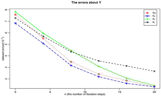
Figure 1. Comparison of the relevant errors in FBSDSs.

We compute $\underset{t\in [t_i,t_{i+1})}{max}|Y_t^{\left(n\right)}-Y_{t_i}^{\pi }|$ for some positive integer n. We denote

$$e_n=max\left\{\right|Y_t^{\left(n\right)}-Y_{t_i}^{\pi }|;t\in [t_i,t_{i+1})\},$$

where $Y_t^{\left(n\right)}$ is the nth iteration of $Y_t$ for Markovian iteration, four steps and layer method; $Y_{t_i}^{\pi }$ is from Euler method. In the results of comparison, We only use the Euler method as a yardstick of comparison, a base method. Due to being numerical methods, the Euler method does not necessarily get the best estimate. Table 1 presented the errors of ${\widehat{Y}}_t$ between the three methods and the Euler method when iteration numbers increase. From the table, these three methods all get similar results, and Markovian iteration is more close to the Euler method.

Table 1. The errors of ${\widehat{Y}}_t$ between the numerical methods and the Euler method on the FBSDEs.

n	1	2	3	4	5	6
Markovian	5.543 × ${10}^4$	3.451 × ${10}^3$	5.786 × ${10}^2$	71.561	3.491 × ${10}^{-2}$	6.562 × ${10}^{-4}$
Four-step	4.641 × ${10}^4$	2.657 × ${10}^4$	4. 891 × ${10}^2$	6.497	4.786 × ${10}^{-2}$	5.578 × ${10}^{-3}$
Layer	1.781 × ${10}^5$	2.476 × ${10}^4$	3. 651 × ${10}^3$	3.581	2.354 × ${10}^{-1}$	3.671 × ${10}^{-3}$

4. Parallel Methods for FD Solutions of BSDEs in Finance

From numerical analysis viewpoint, challenging problems are the search for fast and efficient simulation schemes of BSEDs. Then the study of application and theory is very important. In the section, we review several given parallel methods to the BSDEs in theory and in application. The idea is to impose the parallel methods on solving some BSDEs, in order to optimize cost and time.

4.1. Multistep Method for the BSDEs in Space-Time

Zhao et al. (2010) proposed a multistep discretization method in space-time to solve Equation (1). To approximate conditional expectations of the equations, they used Lagrange interpolating polynomials, and the Gauss-Hermite quadrature. Some examples were given, including an evaluation problem in stock markets.

From the structure of the method, its FD procedures among space grids are independent. Thus, parallel computing techniques can be adopted to solve large scale problems. Zhang (2010) gave some examples of parallel computing in his thesis.

4.2. Schwarz Waveform Relaxation for FBSDEs in Space-Time

Waveform relaxation (WR) can be performed in parallel computers, in order to solve large-scale equations. The WR methods are mostly based on block Jacobi, Gauss-Seidel or Schwarz methods. For the WR solution, many works are related to convergence theory, acceleration methods, and parallel implementation. In the same time, to decrease computation time, many researchers proposed parallelization in finance, see, Sak et al. (2007). Schwarz WR methods are easy parallel methods, and converge faster than the nomal Schwarz methods (Gander 2006). More recently, Schwarz methods have also been used to solve the BSDEs, see also Tran (2011).

Tran (2011) reconstructed the four step method with some novel conditions to the FBSDEs in Equation (23), and associated it with Schwarz WR to solve Equation (25). Generically, Schwarz method partitions a solution space into the subspaces. The method has two main advantages: it is global in time, and does not conform space-time discretization in different subdomains, and few iterations are used to obtain an accurate solution, due to some suitable conditions.

4.3. Block Allocation for the BSDERs in Finance

Though many methods have been made to obtain the FD solutions of the BSDERs, little work has been done on parallel method. Time constraints are often respected in financial problems, and the implementations are in many costs. Peng et al. (2010) developed a parallel method for the BSDERs, to option pricing. The method is a parallel method with block allocation, and about Peng and Xu (2008) method for the BSDEs.

Peng and Xu (2008) considered the FD methods of the standard BSDEs (1), $[0,T]$ is divided into n time steps in $\delta =T/n$. The Brownian motion can be approximated with:

$$B_t=\sqrt{\delta }\sum _i{\epsilon }_i^{\pi },$$

where ${\epsilon }_i^{\pi }$ is a Bernoulli sequence. They obtained a FD solution by the following discrete BSDEs on the small interval $[i\delta ,(i+1\left)\delta \right]$,

$$Y_{t_i}^{\pi }=Y_{t_{i+1}}^{\pi }+f(t_i,Y_{t_i}^{\pi },Z_{t_i}^{\pi })\delta -Z_{t_i}^{\pi }{\epsilon }_{i+1}^{\pi }\sqrt{\delta }.$$

(31)

We can see the equation above is similar to (9).

Let $Y_{+}=Y_{t_{i+1}}^{\pi }{|}_{{\epsilon }_{i+1}^{\pi }=1}$ and $Y_{-}=Y_{t_{i+1}}^{\pi }{|}_{{\epsilon }_{i+1}^{\pi }=-1}$. Under some assumptions, the equation above is thus equivalent to the following equations:

$$\begin{array}{cc}\hfill Y_{t_i}^{\pi }& =Y_{+}+f(t_i,Y_{t_i}^{\pi },Z_{t_i}^{\pi })\delta -Z_{t_i}^{\pi }\sqrt{\delta },\hfill \\ \hfill Y_{t_i}^{\pi }& =Y_{-}+f(t_i,Y_{t_i}^{\pi },Z_{t_i}^{\pi })\delta -Z_{t_i}^{\pi }\sqrt{\delta }.\hfill \end{array}$$

(32)

This is equivalent to

$$\begin{array}{cc}\hfill Y_{t_i}^{\pi }& =\frac{1}{2}(Y_{+}+Y_{-})+f(t_i,Y_{t_i}^{\pi },Z_{t_i}^{\pi })\delta ,\hfill \\ \hfill Z_{t_i}^{\pi }& =\frac{1}{2\sqrt{\delta }}(Y_{+}-Y_{-}).\hfill \end{array}$$

(33)

We suppose that $Y_{+}=Y_{t_i}^{t_{i+1}}$ and $Y_{-}=Y_{t_{i+1}}^{t_{i+1}}$, then $Y_{t_i}^{\pi }=Y_{t_i}^{t_i},Z_{t_i}^{\pi }=Z_{t_i}^{t_i}$. By the Equation (33), Peng et al. (2010) get a following explicit scheme. It is performed from level $n-1$ to level 0 of the following binomial tree model

$$\begin{array}{cc}\hfill Y_{t_i}^{t_i}& =\frac{1}{2}(Y_{t_i}^{t_{i+1}}+Y_{t_{i+1}}^{t_{i+1}})+f(t_i,Y_{t_i}^{t_i},Z_{t_i}^{t_i})\delta ,\hfill \\ \hfill Z_{t_i}^{t_i}& =\frac{1}{2\sqrt{\delta }}(Y_{t_i}^{t_{i+1}}-Y_{t_{i+1}}^{t_{i+1}}).\hfill \end{array}$$

(34)

This is the equation, performed by block allocation.

The discussed method uses task decomposition to parallelize the BSDEs by block allocation, the parallel method does not have a linear speed-up rate, since the computation of block allocation method can not be done with embarrassing parallelism. But the method gave a chance to improve the execution time of the BSDERs.

To get the solution of the BSDEs, Dai et al. (2010) used GPU to speed up option pricing computations with the BSDEs. It is shown that, when the numbers of simulations are small, the speedups seem insignificant. Moreover, higher accuracy will be achieved when the value of them increases. Gobet et al. (2016) concern parallelization and the use of GPUs.

Now, we give a comparison of the three methods on the BSDEs as follows. For the following equation, $f(t,Y_t,Z_t)=t+2Y_t+3Z_t$ in Equatioins (1) and (22), the same initial values are also given. We denote

$$e_n=max\left\{\right|Y_t^{\left(n\right)}-Y_{t_i}^{\pi }|;t\in [t_i,t_{i+1})\},$$

where $Y_t^{\left(n\right)}$ is the nth iteration of $Y_t$ for Multistep method, Schwarz WR and block allocation; $Y_{t_i}^{\pi }$ is from Euler method.

We examine the performance of these method in the BSDEs. In the results of comparison. Here we only use the Euler method a base method. Table 2 shows the errors of ${\widehat{Y}}_t$ between these methods and the Euler method when iteration numbers increase. From the table, Multistep method is more close to the Euler method.

Table 2. The errors between the three methods and the Euler method on the BSDEs.

n	1	2	3	4	5	6
Multistep method	5.546 × ${10}^4$	7.675 × ${10}^3$	4.453 × ${10}^2$	3.448	8.473 × ${10}^{-2}$	3.651 × ${10}^{-4}$
Schwarz WR	4.658 × ${10}^4$	6.781 × ${10}^4$	2.614 × ${10}^2$	4.323	7.654 × ${10}^{-2}$	4.548 × ${10}^{-3}$
Block allocation	1.784 × ${10}^5$	3.816 × ${10}^4$	2.657 × ${10}^3$	7.673	4.564 × ${10}^{-1}$	3.445 × ${10}^{-3}$

5. Discussion and Conclusions

This paper has reviewed many developments in numerical solution of the BSDEs. Numerical solution of BSDE-based mathematical models have been an important research topic over decades. Over the last decade, the BSDEs have been studied intensively, and a vast related literature conduct academic research, and provide practical assistance in financial problems. Numerical solutions of the BSDEs have made recent progresses in finance problems. Although some numerical methods of BSDEs have been proposed, they suffer the problem of complexity, or are very costly. As for the BSDEs, there is a large potential applicability for other economics and finance problems such as game theory, credit risk or liquidity risk models. Motivated in particular by the BSDEs, one faces challenging numerical problems. For example, they are arising in high dimension finance, partial information, transaction costs and so on.

To address these issues in financial problems, the inference development present new challenges. Especially, distributed method (or parallel method) should now become hot topic.

References

- Antonelli, Fabio, and Andrea Pascucci. 2002. On the viscosity solutions of a stochastic differential utility problem. Journal of Differential Equations 186: 69–87. [Google Scholar] [CrossRef]
- Bally, Vlad, and Gilles Pages. 2002. A quantization algorithm for solving discrete time multidimensional optimal stopping problems. Bernoulli 9: 1003–49. [Google Scholar] [CrossRef]
- Bally, Vlad, and Gilles Pages. 2003. Error analysis of the quantization algorithm for obstacle problems. Stochastic Processes and their Applications 106: 1–40. [Google Scholar] [CrossRef]
- Bender, Christian, and Jianfeng Zhang. 2008. Time discretization and markovian iteration for coupled FBSDEs. Annals of Applied Probability 18: 143–77. [Google Scholar] [CrossRef]
- Bender, Christian, and Thilo Moseler. 2010. Importance sampling for backward SDEs. Stochastic Analysis and Applications 28: 226–53. [Google Scholar] [CrossRef]
- Bender, Christian, and Robert Denk. 2007. A forward scheme for backward SDEs. Stochastic Processes and their Applications 117: 1793–812. [Google Scholar] [CrossRef]
- Bouchard, Bruno, and Nizar Touzi. 2004. Discrete time approximation and Monte Carlo simulation for backward stochastic differential equations. Stochastic Processes and their Applications 111: 175–206. [Google Scholar] [CrossRef]
- Bouchard, B., and J. Chassagneux. 2008. Discrete-time approximation for continuously and discretely reflected BSDEs. Stochastic Processes and their Applications 118: 2269–93. [Google Scholar] [CrossRef]
- Bouchard, Bruno, and Romuald Elie. 2008. Discrete time approximation of decoupled forward-backward SDE with jumps. Stochastic Processes and their Applications 118: 53–75. [Google Scholar] [CrossRef]
- Chassagneux, Jean-François. 2009. Discrete-time approximation of doubly reflected BSDEs. Advances in Applied Probability 41: 101–30. [Google Scholar] [CrossRef][Green Version]
- Chevance, D. 1997. Numerical methods for backward stochastic differential equations. In Numerical Methods in Finance. Edited by L. C. G. Rogers and D. Talay. Cambridge: Cambridge University Press, pp. 232–44. [Google Scholar]
- Cheridito, Patrick, H. Mete Soner, Nizar Touzi, and Nicolas Victoir. 2007. Second Order Backward Stochastic Differential Equations and Fully Non-Linear Parabolic PDEs. Communications in Pure and Applied Mathematics 60: 1081–110. [Google Scholar] [CrossRef]
- Crisan, Dan, Konstantinos Manolarakis, and Nizar Touzi. 2010. On the Monte Carlo simulation of BSDEs: An improvement on the Malliavin weights. Stochastic Processes and their Applications 120: 1133–58. [Google Scholar] [CrossRef]
- Dai, Bin, Ying Peng, and Bin Gong. 2010. Parallel Option Pricing with BSDE Method on GPU, gcc. Paper present at Ninth International Conference on Grid and Cloud Computing, Nanjing, China, November 1–5; pp. 191–95. [Google Scholar]
- Delarue, François, and Stéphane Menozzi. 2006. A forward-backward stochastic algorithm for quasi-linear PDEs. Annals of Applied Probability 16: 140–84. [Google Scholar] [CrossRef][Green Version]
- Douglas, Jim, Jin Ma, and Philip Protter. 1996. Numerical methods for forward–backward stochastic differential equations. Annals of Applied Probability 6: 940–68. [Google Scholar] [CrossRef]
- El Karoui, Nicole, Shige Peng, and Marie Claire Quenez. 1997. Backward stochastic differential equations in finance. Mathematical Finance 7: 1–71. [Google Scholar] [CrossRef]
- Elie, R., and I. Kharroubi. 2010. Probabilistic representation and approximation for coupled systems of variational inequalities. Statistics & Probability Letters 80: 1388–96. [Google Scholar]
- Essaky, E. H. 2008. Reflected backward stochastic differential equation with jumps and RCLL obstacle. Bulletin of Mathematical Sciences 132: 690–710. [Google Scholar] [CrossRef]
- Gander, M. J. 2006. Optimized schwarz methods. SIAM Journal on Numerical Analysis 44: 699–731. [Google Scholar] [CrossRef]
- Gobet, Emmanuel, and Céline Labart. 2010. Solving BSDE with adaptive control variate. SIAM Journal on Numerical Analysis 48: 257–77. [Google Scholar] [CrossRef]
- Gobet, Emmanuel, Jean-Philippe Lemor, and Xavier Warin. 2005. A regression based Monte Carlo method to solve backward stochastic differential equations. Annals of Applied Probability 15: 2172–202. [Google Scholar] [CrossRef]
- Gobet, Emmanuel, and Céline Labart. 2007. Error expansion for the discretization of backward stochastic differential equations. Stochastic Processes and their Applications 117: 803–29. [Google Scholar] [CrossRef]
- Gobet, Emmanuel, J. López-Salas, P. Turkedjiev, and C. Vázquez. 2016. Stratified regression Monte-Carlo scheme for semilinear PDEs and BSDEs with large scale parallelization on GPUs. SIAM Journal on Scientific Computing 38: 652–77. [Google Scholar] [CrossRef]
- Kharroubi, Idris, Jin Ma, Huyên Pham, and Jianfeng Zhang. 2010. Backward SDEs with constrained jumps and quasi-variational inequalities. Annals of Probability 38: 794–840. [Google Scholar] [CrossRef]
- Kobylanski, M. 2000. Backward stochastic differential equations and partial differential equations with quadratic growth. Annals of Probability 28: 558–602. [Google Scholar] [CrossRef]
- Lemor, Jean-Philippe, Emmanuel Gobet, and Xavier Warin. 2006. Rate of convergence of an empirical regression method for solving generalized backward stochastic differential equations. Bernoulli 12: 889–916. [Google Scholar] [CrossRef]
- Ma, Jin, Philip Protter, Jaime San Martin, and Soledad Torres. 2002. Numerical methods for backward stochastic differential equations. Annals of Applied Probability 12: 302–16. [Google Scholar]
- Ma, Jin, Philip Protter, and Jiongmin Yong. 1994. Solving forward-backward stochastic differential equations explicitly-a four step scheme. Probability Theory and Related Fields 98: 339–59. [Google Scholar] [CrossRef]
- Ma, Jin, Jie Shen, and Yanhong Zhao. 2008. On numerical approximations of forward-backward stochastic differential equations. SIAM Journal on Numerical Analysis 46: 2636–61. [Google Scholar] [CrossRef]
- Ma, Jin, and Jianfeng Zhang. 2005. Representations and regularities for solutions to BSDEs with reflections. Stochastic Processes and Their Applications 115: 539–69. [Google Scholar] [CrossRef]
- Makarov, R. 2003. Numerical solution of quasilinear parabolic equations and backward stochastic differential equations. Russian Journal of Numerical Analysis and Mathematical Modelling Rnam 18: 397–412. [Google Scholar] [CrossRef]
- Milstein, G. N., and M. V. Tretyakov. 2006. Numerical algorithms for forward-backward stochastic differential equations. SIAM Journal on Scientific Computing 28: 561–82. [Google Scholar] [CrossRef]
- Peng, Ying, Bin Gong, Hui Liu, and Yanxin Zhang. 2010. Parallel Computing for Option Pricing Based on the Backward Stochastic Differential Equation. In High Performance Computing and Applications (Lecture Notes in Computer Science). Berlin: Springer, vol. 5938, pp. 325–30. [Google Scholar]
- Peng, Shige, and Mingyu Xu. 2008. The Numerical Algorithms and simulations for BSDEs (2008). ArXiv, arXiv:08062761. [Google Scholar]
- Peng, Shige, and Zhen Wu. 1999. Fully Coupled Forward-Backward Stochastic Differential Equations and Applications to Optimal Control. SIAM Journal on Control and Optimization 37: 825–43. [Google Scholar] [CrossRef]
- Peng, S., and Z. Yang. 2009. Anticipated backward stochastic differential equations. Annals of Probability 37: 877–902. [Google Scholar] [CrossRef]
- Royer, Manuela. 2006. Backward stochastic differential equations with jumps and related nonlinear expectations. Stochastic Processes and Their Applications 116: 1358–76. [Google Scholar] [CrossRef]
- Rouge, Richard, and Nicole El Karoui. 2000. Pricing via utility maximization and entropy. Mathematical Finance 10: 259–76. [Google Scholar] [CrossRef]
- Sak, Halis, Súleyman Ózekici, and Ílkay Bodurog. 2007. Parallel Computing in Asian option pricing. Parallel Computing 33: 92–108. [Google Scholar] [CrossRef]
- Situ, Rong. 1997. On solution of backward stochastic differential equations with jumps. Stochastic Processes and their Applications 66: 209–36. [Google Scholar]
- Situ, Rong, and Juliang Yin. 2003. On solutions of forward-backward stochastic differential equations with Poisson jumps. Stochastic Analysis and Applications 21: 1419–48. [Google Scholar]
- Tran, Minh-Binh. 2011. A parallel four step domain decomposition scheme for coupled forward backward stochastic differential equation. Journal de Mathématiques Pures et Appliquées 96: 377–94. [Google Scholar] [CrossRef][Green Version]
- Zhang, Jianfeng. 2004. A numerical scheme for BSDEs. Annals of Applied Probability 14: 459–88. [Google Scholar] [CrossRef]
- Zhang, Guannan. 2010. An Accurate Numerical Method for High Solving Backward Stochastic Differential Equations. Master’s thesis, Shandong University, Jinan, China. [Google Scholar]
- Zhao, Weidong, Guannan Zhang, and Lili Ju. 2010. A stable multi-step scheme for solving backward stochastic differential equations. SIAM Journal on Numerical Analysis 48: 1369–94. [Google Scholar] [CrossRef]
- Zhu, Xuehong. 2010. Backward stochastic viability property with jumps and applications to the comparison theorem for multidimensional BSDEs with jumps. ArXiv, arXiv:1006.1453. [Google Scholar]
© 2018 by the author. Licensee MDPI, Basel, Switzerland. This article is an open access article distributed under the terms and conditions of the Creative Commons Attribution (CC BY) license (http://creativecommons.org/licenses/by/4.0/).