Abstract
Assuming that a time series incorporates “signal” and “noise” components, we propose a method to estimate the extent of the “noise” component by considering the smoothing properties of the state-space of the time series. A mild degree of smoothing in the state-space, applied using a Kalman filter, allows for noise estimation arising from the measurement process. It is particularly suited in the context of a reputation index, because small amounts of noise can easily mask more significant effects. Adjusting the state-space noise measurement parameter leads to a limiting smoothing situation, from which the extent of noise can be estimated. The results indicate that noise constitutes approximately 10% of the raw signal: approximately 40 decibels. A comparison with low pass filter methods (Butterworth in particular) is made, although low pass filters are more suitable for assessing total signal noise.
1. Introduction
Practical ways to measure reputation have advanced rapidly in the past few years with the increased use of internet data feeds. As with any measurement that involves a physical apparatus, error is induced in such a measurement by the measurement process itself. The purpose of this paper is to estimate the extent of the error induced by the process of collecting and analysing sentiment data to produce a reputational time series. It is often argued that it is important for an organisation to maintain a “good reputation”, but two questions are commonly left unanswered. The first is the question of what precisely is meant by the term “reputation”. The second is how to measure it. For an example of this approach, see Deloitte (2016). A slight advance is exemplified by Cole, in which reputation is determined by survey, and reputational effects are noted using changes in balance sheet items. The first of these questions has been addressed in detail in Mitic (2017a). The second was answered in Mitic (2017b). To provide a context for the main discussion of this paper, the results of those two papers will be summarised below. Given that reputation can be measured, the measure becomes meaningful in commercial terms only when expressed in monetary terms. A conversion in terms of annual company sales and profit was estimated in Mitic (2017b), thereby justifying the effort and expenditure that is often directed at maintaining a positive reputation. The error induced in a measure of reputation by the process of measurement therefore translates into an error in associated monetary risk. The amount of this error is estimated in the final part of this paper. Three methods for estimating the amount of noise in reputational time series are described and compared. The State-Space (Kalman filter) method is the principal method, and it is compared with a simple low pass filter (Moving Average), and a more complex low pass filter (Butterworth). Such low pass filters are more suited to assessing the total signal noise because they do not have a dedicated parameter that controls measurement noise, as does the Kalman filter. Nevertheless, low pass filters give an overall indication of signal noise. The terms time series and signal are used interchageably in this paper, the terms being used to mean the same thing in the worlds of statistics and signal processing, respectively.
2. Reputation and Its Measurement
This section contains a summary of the main points in Mitic (2017a) and Mitic (2017b). The process of reputation measurement is a relatively recent development, made possible by exploiting internet connectivity and advances in sentiment analysis.
2.1. Definitions for Sentiment and Reputation
Consider a set of agents (individuals or groups) that comment on a target organisation G at time t. Those comments can be analysed and each can be given a score in the range [−1, 1]. See Liu (2015) for a full discussion of how such a score may be derived. A score near 1 means that the agent who expressed the comment is very favourably disposed towards G. A score near −1 means exactly the opposite, and a score of 0 means that the agent’s position with respect to G is neutral. The range [−1, 1] is arbitrary, but it makes intuitive sense to cast the score in terms of positive and negative numbers.
To be more precise, let H (for Holder) denote an agent who makes a comment at time t, and denote the corresponding score by , where i is a unique identifier for the comment. Next, consider a collection of scored comments , in which T is an indexing set for times and I is an indexing set for unique identifiers. The reputation of organisation G at time t, , can then be defined as a weighted average of the scores in such a collection. To this end, let be the weight of comment i. Then, , can be expressed as:
The weights are arbitrary, but represent some appropriate characteristic of the holder of the corresponding score . For example, could represent the influence of H. A high (positive) weight indicates a very influential holder (for example, a national newspaper) and low (positive) weight indicates an uninfluential holder (for example, a Twitter user with only a few followers). For example, a Twitter user with 100 or fewer followers is assigned weight 1. A Twitter user with 1 million or more followers is assigned weight 10. Other uses are weighted on a linear scale based on the two fixed points defined by those users. The number of followers for each user under consideration is determined dynamically. Similarly, for traditional media, the weights are based on circulation and viewer figures for newspapers and broadcasts, respectively. Note that Equation (1) applies only at a single time t. It is only a single snapshot. More generally, the reputation of G is formally defined as a time series, (Equation (2)).
We stress that Equation (2) does not account for opinion formulation on the basis of only a few (perhaps only one) received comments. This is a form of “reputation” that sometimes appears in informal discourse, and is not appropriate for the analysis in this paper.
2.2. Sentiment Procurement
Figure 1 shows an overview of the data mining and analytical stages in sentiment procurement. Proceeding from left to tight in the figure, the stages are:
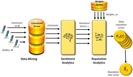
Figure 1.
The stages in the process of reputation measurement.
- Receive “comments” electronically from opinion holders, H, that convey sentiment with respect to a target G from public sources (news channels, social media, etc.).
- Sentiment analysis for each comment, to give a sentiment “score”, nominally in the range [−1, 1].
- For each comment, define a weight (e.g., to reflect the influence of the opinion holder of the comment).
- Compose a reputation index applicable at a particular time using all the sentiment scores received in a given time period (such as one day). This is Equation (1).
- Accumulate successive time-based reputation indexes to form the reputation time series, of Equation (2).
The result is a single number per time period (in practice daily) that measures the reputation of the target organisation, G. The approach indicated above was pioneered by the London business intelligence consultancy Alva Group (www.alva-group.com). The precise calculation of the elements in Equation (1) is more complex than indicated here, and is not publicly available.
The short series, S, i.e., Equation (3), shows a few examples of the result of the process shown in Figure 1 (Ford Motors, starting on 1 July 2015, adapted from data from Alva Group). Positive and negative numbers correspond ,respectively, to positive and negative sentiment.
The entries in Equation (3) show some numbers with relatively high absolute values, and a few that are close to zero. The latter are the subject of this paper. This point will be explored in more detail shortly in this paper.
2.2.1. Reputation and Financial Risk
Basic definitions of sentiment and reputation were given in Mitic (2017a). The essential premise of that paper is that reputation can be expressed in terms of monetary units (GBP, USD, EUR, etc.). The finding differentiated between three operational cases. The first is a “business as usual” (BAU) context, in which there are no major reputational shocks. The second is the “stressed” context, in which a significant reputational event results in a noticeable change in the values in the reputation index following the event. The third is the “super-stressed” context, in which a very significant reputational event results in a prolonged and deep change to the profile of the reputation index. An example of a “super-stressed” event is the Volkswagen emissions revelation in September 2015. See Jung and Park (2016) or the wiki entry (https://en.wikipedia.org/wiki/Volkswagen_emissions_scandal) for an account of the history of this affair. The conversions from accumulated annual reputation to profit after tax are shown in Table 1.

Table 1.
Effect of annual reputation change on profit after tax.
In the analysis that follows, a convenient risk metric, and also a telling visual illustration, is to calculate the cumulative reputation, , which is the set of cumulative sums of the reputation scores in . With the indexing set T for times t:
The way in which changes with small changes in particular values of can be expressed in monetary terms. This is the methodology proposed in Section 3 to assess the effect of measurement error in values of .
2.2.2. Reputation Measurement Error
There is an induced error in measuring reputation in the way described above due to data collection and sentiment analysis of that data. A small error or change in the detailed sentiment assessment for a component of a term can reverse the sign of , provided that the value of is very marginally positive or very marginally negative. The purpose of this study is to assess the extent of this error and to calculate how much it is worth in monetary terms. This permits an error bound on to be calculated in the following way. First assume that a set of very marginal negative reputation values should, in fact, have been positive. Changing their signs from negative to positive then increases the proportion of positive sentiment scores that enter the calculation of . Similarly, a set of sentiment scores, incorrectly recorded as positive, could have their signs changed to negative, and thereafter be treated as negative scores. This would then increase the proportion of negative components values in . The process of transferring negative sentiment values to positive, and positive to negative, followed by a recalculation of in the two cases, allows us to estimate an upper and a lower bound on the value of induced by the measurement process. The monetary value of those error bounds can then be estimated.
As a simple example, consider the second reputation score, −0.0036, in S (Equation (3)), which is close to zero. Suppose that the weighted components of that sum are 0.245, 0.109, −0.078, −0.27, −0.0122. Suppose, further, that a change to the sentiment analysis algorithm results in a small change to one of these components. For example, the first component, 0.245 changes to 0.260. That is enough to change the sum of the five components from negative to a positive value, 0.0088, thereby reversing the sign and sense of the reputation score. Alternatively, suppose that a change to the data collection procedure results in an additional weighted component, 0.007. When the six components are summed, the result is 0.0008, again reversing the overall sign and sense of the reputation score.
Following this numerical illustration, we now discuss the detailed algebraic implementation of a method to calculate measurement error bounds.
3. Methodology
The methodology used to assess the inherent measurement error described in the previous section is to apply a smoothing filter to the times series to isolate, objectively, a set of positive and negative values of that are in the neighbourhood of zero. The upper bound is then obtained by mapping the negative values in that neighbourhood to a positive value, thereby boosting the cumulative reputation, . Similarly, the lower bound is obtained by mapping the positive values in that neighbourhood to a negative value, thereby reducing the cumulative reputation. State space smoothing is the preferred method used to achieve the above objectives. The reasons are given in the next sub-section. The following subsections contain a summary of the state-space methodology, and the specialisations of it applicable to the task in hand. The State-Space method is one of many methods that filter parts of a signal. We associate noise with the high frequency parts of a signal, and aim to remove that noise using the filter. The Kalman filter is associated with the State-Space method. More generally, we also consider removal of high frequency noise using other low pass. They are designed to transmit the low frequency parts of the signal, and to block the high frequency parts. In general we are less confident in using low pass filtering for our purpose because they have no specific parameter to assess measurement noise.
3.1. Nomenclature
For the purposes of this paper, a time series received from a source without further processing or analysis will be referred to as an Observed Signal. Such an Observed Signal comprises two components: an Unobserved Signal, which is the part we would like to discover, and Noise. The Unobserved Signal and the Observed Signal at time t will be denoted by the symbols and , respectively. In the uni-dimensional state-space analysis that follows, both and are scalars, but more generally they are vectors.
3.2. The State-Space and the Kalman Filter
State space analysis, otherwise known as “dynamic linear modelling”, originates from the work of Kalman (1960) in the context of tracking the position (i.e., the state) of a spacecraft with location , given a noisy location measurement . is termed the state vector. It contains all available information to describe the investigated system, and is usually multidimensional. The measured vector, , represents observations related to the state vector. is often of lower dimension than the state vector. The idea that some quantity has a value which we can estimate by measuring is central to the argument in this paper. Measuring reputation by collecting expressed sentiments electronically is not exact. A certain amount of expressed sentiment constitutes “noise” in the sense that the sentiment is expressed routinely such that it does not reflect any significant event. Chapter 6 in Shumway and Stoffer (2017) is a good account of the Kalman filter in the context of state-space analysis, and the summary that follows is based on it. The Kalman filter can be used for any of three purposes: prediction, filtering and smoothing. We exploit the latter here. The name filter should be thought of as a filtering out of noise (i.e., noise reduction, not elimination). A useful phrase summarising Kalman filtering is:
Noisy signal in: less noisy signal out
The Kalman filter technique is used in the context of reputational analysis for three main reasons:
- Kalman filtering incorporates a specific smoothing parameter which can be used to assess measurement noise. Other smoothing methodologies (e.g., Loess filter and moving average) do not have such a specific relationship with measurement.
- Construction of the reputation index (specifically resetting to an initial value every period) produces a signal for which a static model with noise is appropriate: there is necessarily no trend and no seasonality. A particularly simple version of the Kalman model is available for precisely this situation.
- Very little lag is introduced by the smoothing process.
- The Kalman filter (state-space) method makes direct use of the distribution of reputation scores, which can be modelled successfully by a Normal distribution.
- The Kalman filter methodology assumes that the time series being analysed is stationary. All of the reputational time series in this study are stationary, as demonstrated by examining their frequency spectra. It is expected that others will also be stationary unless they are driven by seasonal events.
3.3. Kalman Filter Fundmentals
Let the current unobserved state of a quantity x at time t be , where t varies discretely in steps of 1 between 0 and a maximum value . In one dimension, this is the single state variable. Then, in terms of the state at the prior time slot t−1,
in which is a control variable that can influence and is, in general, a control matrix which maps controls to state variables. is a stochastic error which is usually taken as , where Q is a correlation matrix measurement of volatility of the state variable itself. Ultimately, we aim to calculate an estimator, , of . The observed variable is related to by Equation (6), in which also appears with another control matrix . The matrix is known as the observation matrix and represents a measurement scaling. There is another stochastic error term which is usually taken as , where R is a measurement error matrix.
In the uni-dimensional case, all matrices in Equation (6) are 1-by-1, so they are scalars.
The Kalman analysis continues by defining a predict and an update stage. Let denote the estimate of state at time t. In addition, let be the variance matrix of the error . The goal is to minimize . The prediction stages for and P are (the superscript T denotes transpose):
The predict stage is initialised with known values for , and for . The corresponding update stage is given in terms of a measurement residual vector , a residual variance matrix , and an innovation part which gives the transition of to in terms of a Kalman gain matrix, :
There is an optimal gain Kalman Filter, defined by
With this , the update equations resolve to:
The three predict Equations (9) and the three update Equations (11) define the basis of the special case that follows.
3.3.1. Kalman Smoothing: The Static Model Specialisation
In this section, we modify the predict and update equations such that they apply to the case where there is effectively a constant noisy signal. In Mitic (2017a) the idea of a standardised reputation score was introduced and developed (SubSection 3.3.1 in this paper has a summary). A daily score in the range [−1, 1] is produced, the range (0, 1] corresponding to positive sentiment and the range [−1, 0) corresponding to negative sentiment. A score of 0 represents completely neutral sentiment, and a score in a neighbourhood of 0 is the noise that we wish to estimate. This score is the observed signal , time t referring to a daily measurement. Details of the physical method of sentiment procurement were also given in SubSection 3.3.1, and a fuller account may be found in Mitic (2017b). In that paper, and also in SubSection 2.1 of this paper, the formal time series definition of the reputation of an organisation G at time t is written as , but the notation serves for the current purpose because it is consistent with much of the notation on state-space analysis in the literature. The methodology is such that the neutral score is the starting point each day.
As such, we regard the resulting reputational time series as measuring deviations from a constant value (namely the neutral score), with, necessarily, no trend and no seasonality. This condition allows us to set the 1-by-1 transition matrix in Equation (7) to 1: . In addition we assume there is no control term, so . The matrix H represents a scaling with respect to the measurement, and is also set to 1 since we make no measurement scaling. The process is a scalar, so P is a scalar. Process noise Q is assumed to be a constant scalar with value q. The same applies for measurement noise, so we set R to a constant scalar value r. The predict Equations (9) and the update Equations (11) then reduce to the following equations for . The smoothing case is for . The case corresponds to filtering and if , the Kalman process is in predictive mode.
Predict:
Update:
3.3.2. Normality Assumption of State-Space Analysis
The state-space methodology, summarised in terms of the Kalman filter, by Equations (9) and (11), and the specialisation in Equations (12) and (13) depend on a normality assumption. Specifically, the elements of the input time series, , must be normally distributed. State space is a linear representation of the dynamic behaviour of , so if is normally distributed, so is its state-space formulation, (Hamilton 1986). Further, the Kalman filter algorithm assumes that the state transitions are linear, and that the error terms when fitting to data are normally distributed. See, for example, Cosma and Evers (2010) or Shumway and Stoffer (2017) for a full discussion of this point. Calculation of confidence limits in the analysis that follows depends on this assumption of normality.
If the input time series is not normally distributed, it is generally possible to apply a transformation such that the transformed series is normally distributed. Generally, power transformations are successful, and in particular the Box-Cox transformation (Equation (14), which depends on selecting a suitable parameter . Using Box-Cox, each element y of is mapped to y’, where
Alternatively, log transformations are often successful in transforming to normal distributions. Many of the input time series used in this analysis have outliers that indicate non-normality. Therefore a Box-Cox transformation has been applied to normalise them sufficiently to permit calculation of confidence limits.
3.3.3. Kalman Filter Noise Estimation
Equations (12) and (13) can now be applied to estimate the noise component in a signal. The first stage is to fix the volatility parameters q and r. Parameter q is taken as the standard deviation of the observed signal. It is assumed to be an intrinsic property of the observed signal, and is therefore fixed. Parameter r represents measurement noise, and is determined by considering a range of appropriate values and choosing one that results in maximum noise, as determined by the method outlined below. Once a value for r has been found, the noise in the observed signal can be isolated using the confidence interval, J, given by Equation (15). In (15), and are the mean and standard deviation respectively of the unobserved (i.e., smoothed) signal , and is the 99% 2-tail critical value on the standard Normal distribution. In addition, recall that is the number of elements in both observed and unobserved time series. The confidence interval is based on the assumed Normal distribution for the unobserved signal once it has been modified by Box-Cox.
The values of and vary with the value of the parameter r. For each r, the number of unobserved signals within the confidence interval J can be identified and counted. Writing and for the sets of observed signals in J and the observed signals not in J, respectively (so that ), the percentage of noise in the unobserved signal, P, is then given by Equation (16). This percentage is taken to be the percentage of noise in the observed signal.
3.4. Low Pass Filter Noise Estimation
The action of a low pass filter is to transmit signals with a frequency lower than a cutoff frequency, and to reject signals with frequencies higher than the cutoff. In signal processing, the word attenuate is used is used in place of “reject”. Using a low pass filter on the reputational signals considered in the paper is based on the assumption that the informative parts of the signal have the more extreme values (near +1 or −1). They correspond to the low frequency part of the signal, simply because there are more of them. Noise is confined to values near to zero. There are many more of them, and we associate those values with high frequency. In principle, it is difficult to link the concept of frequency in the context of a reputation signal with the way “frequency” is used in the context of an audio signal. Audio signals are generally treated as superpositions of sinusoidal sub-signals in the form of a Fourier series. This approach has not been hitherto been applied to a reputation signal. We attempt to estimate the amount of noise by filtering out the high frequency noise. In general, low pass filters have only one parameter available for controlling which frequencies are filtered out. Therefore, they filter out all noise, not just measurement noise. They are therefore not as suitable as a means to assess measurement noise, but it is interesting to see the results of using this type of filter. Smith (2007) (Chapter 1) has a simple account of how a low pass filter is intended to work, and Hamming (1989) has a more rigourous account. Practical guidance on programming digital filters using Matlab may be found in Jackson (1996). In principle, any method of smoothing a time series can be used as a filter. None has a dedicated parameter for measurement noise, so they are not as suitable as the Kalman filter for our purposes. The following sections concentrate on two: Butterworth, (Butterworth (1930)), because the low pass property is easy to define, and Moving Average, as a simple comparison.
The overall way in which a digital filter works is to define a new series by applying a transformation to (Equation (17)). Thus, if the filtered signal is ,
Figure 2 illustrates the use of a low pass filter. The solid line shows an ideal state where frequencies less than a cutoff frequency are transmitted, and where no frequencies greater than or equal to are transmitted. The vertical axis shows the gain, which is the ratio of the amplitude of the output signal to the input signal. The “ideal state” filter is shown in red. The horizontal portion corresponding to frequencies f where , and is also shown. All frequencies in that range are transmitted with no degradation in amplitude, shown by gain = 1. The gain for is zero because, ideally, no signal is transmitted in that range. The “non-ideal state” filter is shown in blue. The gain is sub-optimal due to signal degradation, the cutoff at frequency is not sharp, and high frequencies are not completely removed. In the context of a reputation signal, frequency is ill-defined. It is replaced by an appropriate parameter of the method used to assess the noise level. The green profile shows a frequency response where there is no clear cutoff. This shows a response that often occurs in practice: see SubSection 3.4.2.
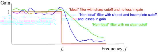
Figure 2.
Ideal (red) and non-ideal (blue) filters, showing gains as a function of Frequency.
3.4.1. The Power Spectral Density (PSD)
The PSD (sometimes called the Power Spectrum) of a signal shows the power in the signal as a function of frequency, per unit frequency. For a discrete signal, power is measured as the square of the signal amplitude divided by the number of signals. A detailed theoretical basis may be found in Stoica (2005). For a simpler treatment, see Cerna (2009). The PSD calculation starts by calculating the Discrete FourierTransform (DFT) of the signal, (Equation (18), in which f is a frequency and n is the number of elements in the series ).
The DFT is a complex number for every f, and its amplitude is given by . Therefore, the PSD is given by the series in Equation (19), in which is a set of frequencies.
The PSD is used in our context to examine the effectiveness of the filtering methodology used. The shape of the PSD is sometimes indicative of a clear noise cutoff level, such that we can regard frequencies above that cutoff as “noise”.
3.4.2. Low Pass Filter Procedures
The steps in the general approach used in applying a low pass filter to a reputation signal are as follows. This approach makes use of the PSD to find a noise cutoff frequency.
- Obtain the PSD for the input signal under consideration
- Determine a cutoff frequency, , by finding the point at which the power spectrum stabilises. All power spectra considered have the property that the power density stabilises at some fraction of the total number of ordinates in the spectrum. Most reputation power spectra exhibit shape frequency profiles similar to the profile illustrated in SubSection 4.2.2. The plot shows a limiting value at frequency 0.7. There is one exception where the spectrum indicated periodicity with period of 100 days (organisation NW in Table 4). This periodicity was likely due to chance, as no reason for it was apparent and it was not observed for other organisation. There is a discussion of special treatment of two other organisations in SubSection 4.3.
- Apply a filter to the input signal using the cutoff frequency to obtain the output signal
- Obtain the PSD for the output signal, . If there are n PSD components , denote the normalised cumulative sums of the square of those components by (squaring emphasises any distinction between low and high frequencies).
Two types of filter will be considered for this analysis. The Butterworth filter aims to achieve an “ideal” filter profile (as in Figure 2). The Moving Average filter is discussed as a comparison.
3.4.3. Moving Average Filter
The Moving Average filter is a very simple form of low pass filter, and is generally used for smoothing time series. When used for filtering, the only parameter that can be used is the number of terms in the moving average. Moving averages introduce lag, so if a very fast response is needed, this may not be an ideal filter method. However, it is very simple to define and implement. If denotes the input time series, the output time series (i.e., the filtered series) of order n, , is given by Equation (21).
The main use of a Moving Average filter in practice is to reduce random white noise while keeping a sharp “ideal” step response, as in Figure 2. There is a discussion of this filter and variations of it in Smith (1999), Chapter 15.
3.4.4. Butterworth Filter
The Butterworth filter is more complex than the Moving Average filter, and is designed to have as flat a frequency response as possible in the pass band (frequencies that should be transmitted), and to block as many frequencies as possible in the stop band (frequencies that should not be transmitted). The pass band can be defined as a frequency range. The useful pass band for the purpose of analysing reputational signals is the range [0, ], where defines a maximum low frequency to be transmitted. Frequencies greater than , which represent noise, should be blocked. A full discussion may be found in, for example, Oppenheim (1989). For such a filter, the square of the amplitude of the filtered signal (termed the Frequency Response), is given by Equation (22), in which the independent variable is the frequency, and n (an integer greater than 1) is the order of the filter. The greater the order, the steeper the response at the cutoff point. The Frequency Response should be as flat as possible for frequencies less than or equal to . Figure 3 shows three examples. The Frequency Response parameter is the only parameter available to control the extent of what is nominally noise. As such the Butterworth filter is less suitable for the purpose of assessing the amount of measurement noise (as opposed to the system noise), but it is worth noting the results of using it as a comparison with the Kalman filter. It should be noted that, in practice, not all frequencies less than or equal to are transmitted, and not all frequencies greater than are blocked. The greatest frequency transmission errors occur near , and for low values filter orders.
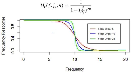
Figure 3.
Examples Butterworth Frequency Responses, critical frequency = 10.
3.5. Signal to Noise Calculation
Expressing the noise level in a time series in terms of the signal to noise () ratio enables a ready comparison with noise in an audio signal, which may be more familiar to some readers. We therefore include a way to measure the ratio using the terms in Equation (16). There are several established ways to calculate a ratio. See, for example, Smith (1999). A convenient method in this context is to use the square of the ratio of the signal amplitude to the noise amplitude. There is a direct implementation in Matlab: the function snr() (see https://uk.mathworks.com/help/signal/ref/snr.html). Thus, if A denotes amplitude,
Expressed in decibels, the ratio is given by .
4. Results
In this section, we present numerical illustrations of the theory in SubSection 3.2 to SubSection 3.5. Reputation data for ten retail UK banks and six UK motor manufacturers provided the observed (i.e., noisy) time signals , of Equation (6). The data covered the period January 2014 to January 2016. To generate normal distributions for each time series, a Box-Cox transformation was first applied to each. It was sufficient to set a common parameter (Equation (14)) to a value derived by aggregating the data from all the time series, and calculating an optimal value. The optimal value was found using package MASS in the R statistical language, which exports a function boxcox. This function fits a Normal distribution to data that have been transformed using trial values of the Box-Cox parameter , using maximum likelihood as the optimisation criterion. The value obtained was = 1.846.
4.1. Kalman Filter Results
The sequence of equations leading to (13) was used to derive values for the unobserved (less noisy) signals, . The process noise parameter, q, was set to the standard deviation of the observed signals . Appendix A gives a justification for using this value, and Appendix B gives parameter values and some details of the calculation methodology. The measurement noise parameter, r, was set to values in the range [0.5, 10.5] in steps of 0.1. Values of r less than 0.5 were excluded because they resulted in minimal smoothing, which did not provide an effective assessment of measurement error. With the indicated range it was possible to achieve a moderate degree of smoothing of the observed signal whilst still preserving the profile of the signal. As an example, Figure 4 shows the first 100 days for both series (the unsmoothed input signal) and (the smoothed output signal) for organisation FT when r is set to 0.7, which is the value that results in maximum noise.
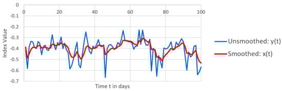
Figure 4.
Example Reputation time series (organisation FT): measured (observed ) and smoothed (unobserved ), with measurement noise parameter set to 0.7. The plots derive from Box-Cox transformed standard reputation signals.
Figure 4 shows that the degree of smoothing is such that the extremes that exist in the observed signal are damped with a minimal lag. The measurement noise to be estimated is in the region near the horizontal line that represents the mean unobserved signal value. For the complete series the mean is −0.379 (indicating an overall negative sentiment towards FT) and for the first 100 entries in the series (shown in Figure 4) the mean is −0.402. Although the theoretical index value can vary between −1 and +1, the observed values are clustered closely about the mean. The only way to attain a perfectly positive score of +1 or a perfectly negative score of −1 would be for all opinion holders to simultaneously express the same perfectly positive or perfectly negative sentiment. Differing opinions among opinion holders results in a reversion towards a zero score.
Figure 5 shows, for organisation FT, how the percentage of noise due to measurement changes as the value of the measurement noise parameter r changes between 0.5 and 10.5. That percentage was calculated from Equation (16) using the confidence interval in Equation (15). Maximum noise is often associated with low values of r. The profile shown is typical.
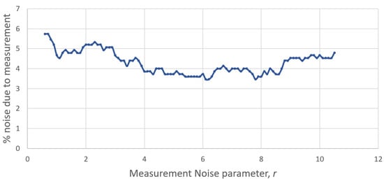
Figure 5.
Variation of percentage of signal noise with measurement noise parameter r: organisation FT.
Table 2 shows the resulting % noise and S/N ratios in decibels for the organisations considered in this study. The entries in the Organisation column are codes to keep the organisations anonymous. The table shows the mean and maximum noise levels as r varies, as well as the S/N values.
Table 2.
Percentage of Noise in Reputation Signals, measured using a Kalman Filter.
An immediate observation from Table 2 is that the noise levels are mostly of the same order, indicating that the results are not merely a feature of the data used. Higher noise levels are largely due to excessive volatility in the observed signal after a major negative reputational hit.
4.2. Low Pass Filter Results
The procedures listed in SubSection 3.4.2, and summarised in Equation (20), were applied separately to each organisation mentioned in the preceding paragraph. Figure 6 is the power spectrum for the unfiltered signal of organisation BS in Table 2. It is a typical power spectrum for reputational signals. The plot shows a limiting cutoff value at frequency ∼0.7, indicating a distinction between “signal” and noise at that point. This indicates that, in the unfiltered signal, the noise level is about 30%. The following subsections show the effects of applying different low pass filters to this, and other, signals.

Figure 6.
Power Spectrum of the Reputation signal for organisation BS, showing limiting cutoff frequency of approximately 0.7.
4.2.1. Low Pass Filter Results: Moving Average Method
The Moving Average filter is a single parameter method that uses the order of the moving average (i.e., the number of elements over which the average is calculated) to control the separation of signal and noise. The results are shown in Table 3. The corresponding S/N values are calculated using the method of SubSection 3.5.
Table 3.
Percentage of Noise in Reputation Signals, measured using a Moving Average Filter. The results are means for moving average orders between 2 and 14 (to cover periods of up to two weeks).
In general, the mean and maximum noise levels for the Moving Average filter are much higher than the corresponding values for the Kalman filter. This is to be expected because the Kalman filter has been configured to estimate the measurement noise as opposed to the system noise, whereas the Moving Average result incorporates both of these. The S/N ratios are all low compared to reasonable audio signals, indicating that noise is a significant component of the total signal. There is much variation in the results between organisations, so that we can summarise the results by noting the Mean entries.
4.2.2. Low Pass Filter Results: Butterworth Method
The Butterworth filter method uses a single parameter to control the separation of signal and noise: the filter order. The mean and maximum noise levels for filter orders between 10 and 25 inclusive was then calculated. These limits provide a reasonably steep cutoff profile (aiming to be similar to the “ideal” filter in Figure 2) without undue complexity. Table 4 shows the results. This table also shows the corresponding S/N values, calculated using the method of SubSection 3.5.
Table 4.
Percentage of Noise in Reputation Signals, measured using a Butterworth Filter. The results are means for filter orders between 10 and 25 inclusive.
Comparing the results in Table 3 and Table 4, it is difficult to settle on any general characteristics that might distinguish the two result sets. In general, the Butterworth filter attributes more noise to the overall signal, although they are of the same order. The implication is that it is sufficient to use a simple filtering method (Moving Average) rather than a more complex method such as Butterworth. The complexities of the latter tend to be embedded in software procedures, whereas code for the Moving Average method is easily visible. The results in Table 4 also show significant variation between organisations. This variation simply reflect differing volatility in the original reputation signal. Overall, the S/N values are higher than for the Kalman filter, but are low in comparison to S/N values encountered in good audio signals (approximately 70–100 db). Further comments are in Section 5.
4.3. Special Treatment of Power Spectra Arising from Reputational Shocks
Two organisations, VOL and HS in Table 3 and Table 4, suffered one severe reputational shock each in the period 2014–2015. They were both involved in illegal activities which were widely reported in the press at the time, and there was much adverse comment on social media. Long-lasting reputational downturns resulted. The power spectra of the unfiltered signals show apparently exceptionally high noise levels in the order of 70%. This does not seem reasonable, and we think that the shock levels are so severe that all non-shock parts of the signal appear to be “noise”. To give a more reasonable estimate of the noise level, the outer quartiles of the signal (i.e., the lowest 25% and the highest 25%) of the scores were excluded from the power spectrum assessment. This process resulted in noise extimates of approximately 80%.
4.4. Monetary Impact
In Mitic (2017b), several results for the monetary effect of reputation are given. We consider, as an illustration, the figures given for monetary gain or loss in stressed circumstances. This is not a “worst case”. It represents either very negative or very positive reputation, but not extreme cases of either, which are very rare. Suppose that, in general, positive reputation accounts for % of profit after tax, and that negative reputation accounts for % of profit after tax. Suppose, further, that the mean maximum and maximum maximum percentage noise levels for filter F considered are and respectively. F takes the values K (for Kalman), B (for Butterworth) or MA (for Moving Average). Then, we attribute percentage monetary amounts with the products and as the mean and maximum noise associated with positive reputation respectively over a one year period. The expressions for negative reputation are similar: is replaced by . In addition to the parameter F for the filter method, let parameter refer to the “mean/max” designation (so it takes values mean or max), and let parameter refer to “positive/negative” reputation (so it takes values “+” or “−”). Then, Equation (24) gives an expression for , the revised percentage monetary value of the reputation component of profit after tax when noise is removed.
The numerical values of the variables used in this section are:
- (from Section 4.1)
- (from Section 4.1)
- (from Section 4.2.2)
- (from Section 4.2.2)
- (from Section 4.2.1)
- (from Section 4.2.1)
- (from Mitic (2017b): Table 5 average)
- (from Mitic (2017b): Table 5 average)
Table 5 gives the values obtained by applying Equation (24) with the numerical values above. Values in the table are given correct to 1 decimal place, which is an appropriate accuracy in this context.
Table 5.
Revised Reputation Contributions to Profit after Tax using mean and Maximum Noise Estimates.
A few points are noteable from Table 5. First, there is very little differentiation between the results for positive and negative reputation, and for the “mean” and “maximum” estimates. That differentiation is much more marked in cases of extreme reputational stress, for which the value of the parameters and are of the order 5% and 10% respectively (see Mitic 2017b, sct. 4.2). Even so, the absolute monetary amount can be substantial. Suppose, for example, that profit after tax is about $500 m. Using the “maximum” Kalman figures from Table 5, positive reputation can add 2.1%, or $10.5 m, to that profit. Negative reputation can remove 2.5%, or $12.5 m from it.
5. Discussion
The aim of this study was to measure the extent of noise in a reputational time series. The Kalman filter is particularly suited for this purpose because it is possible to adjust a filtering parameter specifically for assessing measurement noise, and because its formulation admits an appropriate simple static model. The limiting nature of the degree of smoothing applied allows us to identify the noise component in the observed signal. The results shown in Table 2 indicate that a figure of about 10% would be a reasonable estimate for a maximum noise level applicable to all data sets considered. The mean noise level, a rounded value for which is 8%, is only slightly less. These estimates arise from setting the critical value for the confidence interval in Equation (15) to 99%. If the 95% critical value is used instead the noise percentages may be reduced by approximately one quarter. The S/N values in Table 2 are extremely low compared to what would be expected of a good audio signal (70–100 decibels). Listening to a reputation signal would be like listening to a whisper in a lot of hiss! The Kalman filter results are compared with those derived from low pass filters, principally using the Butterworth filter. Filters other than Kalman do not really assess the amount of measurement noise: they measure total noise. Consequently they are not as suitable as the Kalman filter in answering the question “How much noise does the measurement process add?”.
Overall, the result is useful because it enables us to identify a neighbourhood of the neutral value of the observed signal that is unreliable. Sentiment in this region conveys very little reputational information, and may be interpreted as “chatter”. These small deviations from the neutral value can therefore be discarded in further analyses.
Acknowledgments
I am grateful for the support of Alva-Group for their continued interest, support, and assistance in the preparation of this paper.
Conflicts of Interest
The author declares no conflict of interest.
Appendix A. Calculation of System Noise Parameter q
Using the standard deviation of the observed signal as an estimate of the process noise in the Kalman analysis may be justified by noting the stability of the volatility of the signal, measured on overlapping time slices. For each organisation, the standard deviation of the reputation scores in 100-day (approximately three months) periods, overlapping by 50 days, were noted. The mean of those standard deviations was then compared with the standard deviation of the scores taken over the entire time. The results are noted in Table A1. They indicate that, to an acceptable degree of accuracy, that the standard deviations are stable over time. Therefore the standard deviation taken over the entire time is a reasonable estimate of process noise.
Table A1.
Comparison of Mean of Time-sliced Standard Deviations and overall Standard Deviation of Reputation Signals.
Table A1.
Comparison of Mean of Time-sliced Standard Deviations and overall Standard Deviation of Reputation Signals.
| Organisation | Mean Time-Sliced SD | Overall SD |
|---|---|---|
| BW | 0.049 | 0.048 |
| FT | 0.078 | 0.076 |
| FD | 0.058 | 0.058 |
| HUD | 0.075 | 0.072 |
| NSS | 0.066 | 0.067 |
| MB | 0.049 | 0.047 |
| VOL | 0.097 | 0.094 |
| BSG | 0.115 | 0.112 |
| RYB | 0.112 | 0.108 |
| NW | 0.108 | 0.099 |
| HX | 0.098 | 0.091 |
| HS | 0.117 | 0.099 |
| LL | 0.143 | 0.135 |
| NT | 0.124 | 0.114 |
| TB | 0.150 | 0.147 |
| VG | 0.141 | 0.137 |
| BB | 0.087 | 0.085 |
| DB | 0.093 | 0.084 |
Appendix B. Kalman Calculation Parameters
Table A2 shows calculated Kalman parameters for each organisation. In that table, column Relative % Error is the relative error , where and are defined in Section 3.2. The Kalman calculations were implemented in Excel, and the maximum likelihood calculations used to calculate the Box-Cox parameter were implemented in R.
Table A2.
Kalman Calculation Parameter Values.
Table A2.
Kalman Calculation Parameter Values.
| Organisation | Relative % Error | Parameter q Estimate | Parameter r Estimate |
|---|---|---|---|
| BM | 1.11 | 0.05 | 7.3 |
| FT | 0.11 | 0.08 | 4.31 |
| FD | 0.82 | 0.06 | 6.53 |
| HUD | 1.26 | 0.07 | 16.04 |
| NSS | 0.56 | 0.07 | 6.18 |
| MB | 0.65 | 0.05 | 8.58 |
| VOL | 0.29 | 0.1 | 4.36 |
| BSG | 0.39 | 0.11 | 10.5 |
| RYB | 0.17 | 0.11 | 5.79 |
| NW | 0.26 | 0.11 | 5.19 |
| HX | 0.29 | 0.1 | 9.83 |
| HS | 0.16 | 0.12 | 6.65 |
| LL | 0.35 | 0.14 | 9.9 |
| NT | 0.2 | 0.12 | 8.08 |
| TB | 0.26 | 0.15 | 7.69 |
| VG | 0.25 | 0.14 | 6.22 |
| BB | 0.28 | 0.09 | 9.19 |
| DB | 0.48 | 0.09 | 4.66 |
References
- Butterworth, Stephen. 1930. On the Theory of Filter Amplifiers. Wireless Engineer 7: 536–41. [Google Scholar]
- Cerna, Michael, and Audrey F. Harvey. 2009. The Fundamentals of FFT-Based Signal Analysis and Measurement, National Instruments Application Note 041. Available online: http://www.ni.com/white-paper/4278/en/ (accessed on 8 November 2017).
- Cosma, Ioana A., and Ludger Evers. 2010. Markov Chains and Monte Carlo Methods: Lecture Notes, Chapter 7; African Institute for Mathematical Sciences (AIMS). Available online: http://www.isn.ucsd.edu/classes/beng260/complab/week2/CosmaEvers2010.pdf (accessed on 6 February 2018).
- Deloitte RiskAdvisory. 2016. Reputation Matters: Developing Reputational Resilience Ahead of Your Crisis. Available online: https://www2.deloitte.com/content/dam/Deloitte/uk/Documents/risk/deloitte-uk-reputation-matters-june-2016.pdf (accessed on 8 November 2017).
- Hamilton, James. 1986. State-space models. In Handbook of Econometrics, Chapter 50. Amsterdam: Elsevier, vol. 4, pp. 3039–80. [Google Scholar]
- Hamming, Richard Wesley. 1989. Digital Filters. Englewood Cliffs: Prentice-Hall, Available online: https://www.dsprelated.com/freebooks/filters/ (accessed on 6 February 2018).
- Jackson, Leland B. 1996. Digital Filters and Signal Processing: With MATLAB Exercises. Boston: Kluwer Academic Publishers. [Google Scholar]
- Jung, Jae C., and Su Bin Park. 2016. Case Study: Volkswagen’s Diesel Emissions Scandal. Thunderbird International Business Review 59: 127–37. Available online: http://onlinelibrary.wiley.com/doi/10.1002/tie.21876/full (accessed on 6 February 2018). [CrossRef]
- Kalman, Rudolph Emil. 1960. A New Approach to Linear Filtering and Prediction Problems. Transactions of the ASME–Journal of Basic Engineering 82: 35–45. [Google Scholar] [CrossRef]
- Liu, Bing. 2015. Sentiment Analysis: Mining Opinions, Sentiments and Emotions. Cambridge: Cambridge University Press. [Google Scholar]
- Mitic, Peter. 2017a. Standardised Reputation Measurement. In Proceedings of the IDEAL 2017, Guilin, China. Edited by Hujun Yin, Yang Gao, Songcan Chen, Yimin Wen, Guoyong Cai, Tianlong Gu, Junping Du, Antonio J. Tallón-Ballesteros and Minling Zhang. Lecture Notes in Computer Science (LNCS). Cham: Springer, vol. 10585, pp. 534–542. [Google Scholar] [CrossRef]
- Mitic, Peter. 2017b. Reputation Risk: Measured. In Proceedings of the Paper present at the Complex Systems May 2017, The New Forest, UK, 23–25 May 2017; Edited by George Rzevski and Carlos Brebbia. Southampton: Wessex Institute of Technology Press. [Google Scholar]
- Oppenheim, Alan V., and Ronald W. Schafer. 1989. Discrete-Time Signal Processing. Upper Saddle River: Prentice Hall. [Google Scholar]
- Shumway, Robert H., and David S. Stoffer. 2017. Time Series Analysis and Its Applications: With R Examples, 4th ed. New York: Springer International, chp. 6. [Google Scholar]
- Smith, Julius Orion. 2007. Introduction to Digital Filters: With Audio Applications. Berlin: W3K Publishing. [Google Scholar]
- Smith, Steven W. 1999. The Scientist and Engineer’s Guide to Digital Signal Processing, 2nd ed. Poway: California Technical Publishing, Available online: http://www.analog.com/en/education/education-library/scientist_engineers_guide.html (accessed on 6 February 2018).
- Stoica, Petre, and Randolph L. Moses. 2005. Spectral Analysis of Signals. Upper Saddle River: Prentice Hall. [Google Scholar]
© 2018 by the author. Licensee MDPI, Basel, Switzerland. This article is an open access article distributed under the terms and conditions of the Creative Commons Attribution (CC BY) license (http://creativecommons.org/licenses/by/4.0/).