Brexit and Uncertainty in Financial Markets

Abstract

This paper applies long-memory techniques (both parametric and semi-parametric) to examine whether Brexit has led to any significant changes in the degree of persistence of the FTSE (Financial Times Stock Index) 100 Implied Volatility Index (IVI) and of the British pound’s implied volatilities (IVs) vis-à-vis the main currencies traded in the FOREX (foreign exchange market), namely the euro, the US dollar and the Japanese yen. We split the sample to compare the stochastic properties of the series under investigation before and after the Brexit referendum, and find an increase in the degree of persistence in all cases except for the British pound-yen IV, whose persistence has declined after Brexit. These findings highlight the importance of completing swiftly the negotiations with the European Union (EU) to achieve an appropriate Brexit deal.

1. Introduction

The decision made by the UK to leave the EU as a result of the referendum held on 23 June 2016, commonly known as Brexit, undoubtedly represents a significant shock to the UK economy. In particular, the resulting increase in uncertainty can be expected to have a significant short-run impact on financial markets as well as sizeable long-run effects on real economic activity owing to substantial structural changes to the economy. The present study focuses on the former; more specifically, it applies long-memory techniques (both parametric and semi-parametric) to examine whether Brexit has led to any significant changes in the degree of persistence of the FTSE 100 Implied Volatility Index (IVI), which is a well-known measure of uncertainty in European financial markets. To obtain further evidence we also examine the British pound’s implied volatilities (IVs) vis-à-vis the main currencies traded in the foreign exchange market (FOREX), namely the euro, the US dollar and the Japanese yen. In all cases we split the sample and compare the stochastic properties of the series under investigation before and after the Brexit referendum. To preview the results, we find an increase in the degree of persistence of the IVI index as well as of the British pound-US dollar IV and the euro-British pound IV, whilst there appears to have been a decrease in the case of the British pound-yen IV.

Investor fear about the consequences of Brexit has already been reflected in some asset prices. In particular, the perception of a higher sovereign default risk has led to higher CDS (credit default swaps) spreads, and the greater uncertainty about future economic and policy developments (see, e.g., Baker et al. 2016a) has been associated with wider sovereign and corporate bond yield spreads as well as higher asset price volatility (Kierzenkowski et al. 2016). Moreover, higher risk premia for the British pound have led to an exchange rate depreciation, and a further fall of the British currency is expected by most analysts.

The time series properties of expected risk indicators are clearly of great interest. One of the most informative is the IVI index, which can be viewed as a “fear” index. It is the European counterpart to the better known VIX index for the Chicago stock market that has been examined in most of the literature. In particular, Whaley (2000) suggests that the VIX can be interpreted as an “investor fear gauge” that reaches higher levels during periods of market turmoil. It is an implied volatility index: the lower its level, the lower demand is from investors seeking to buy protection against risk and thus the lower is the level of market fear. Most papers analysing the VIX have focused on its predictive power for future returns (e.g., Giot 2005; Guo and Whitelaw 2006; Chow et al. 2014, 2016; Heydon et al. 2000). Fleming et al. (1995) were the first to analyse the persistence of this index and found that its daily changes follow an AR(1) process, whilst its weekly changes exhibit mean reversion, and there is no evidence of seasonality. Long-memory behaviour in the VIX was also detected by Koopman et al. (2005), Corsi (2009) and Fernandes et al. (2014), as well as by Huskaj (2013) in its volatility. By contrast, Chen and Huang (2014) found no evidence of long memory. Finally, Caporale et al. (2017) used two different long-memory approaches (R/S analysis with the Hurst exponent method and fractional integration) to assess the persistence of the VIX index over the period 2004–2016, as well as some sub-periods (pre-crisis, crisis and post-crisis). They found that its properties change over time: in normal periods, the VIX exhibits anti-persistence (there is a negative correlation between its past and future values), whilst during crises its persistence increases.

In the present paper we analyse the effects of Brexit on the IVI index to assess the extent to which the former has generated more persistent “fear” in financial markets. Since the companies included in the FTSE 100 index make the majority of their profits outside the UK, we extend our analysis to the British pound’s implied volatilities (IVs) in order to obtain a more complete picture—in fact, the suggestion has been made by analysts that Brexit might have more pronounced and long-lasting effects on the FOREX rather than on stock markets.

The layout of this paper is as follows. Section 2 describes the data, Section 3 outlines the methodology and discusses the empirical findings. Section 4 offers some concluding remarks.

2. Data Description

Our sample consists of daily (end-of-the-day) observations on the following four time series: the FTSE 100 Implied Volatility Index (IVI), the 3-month British pound-US dollar IV, the 3-month euro-British pound IV, and the 3-month British pound-Japanese yen IV. For the sake of brevity, henceforth we shall denote the latter three series as GBP-USD IV, EUR-GBP IV and GBP-JPY IV respectively.

The FTSE 100 IVI is a series that measures the implied volatility of the underlying FTSE 100 index. In particular, the IVI is an interpolation of 30, 60, 90, 180, and 360 day implied volatility estimates, which are based on the prices of out-of-the-money options. As a result, the IVI provides an estimate of the market’s volatility expectations on the underlying index between now and the index options’ expiration, and therefore provides useful information to market participants for the purpose of risk management. It is forward-looking, and can be seen as an indicator of market sentiment/fear. Similarly, the British pound’s IV series are measures of markets expectations of volatility conveyed by option prices. In particular, the British pound’s IV series measure the market’s expectation of volatility implied in the prices of the corresponding (at-the-money) currency options over a given time horizon, which is three months in our case. For example, the 3-month British pound-US dollar option gives the right to exchange British pounds for US dollars depending on the expected swings in the former vis-à-vis the latter over the following 90 days.

All the series are from Thomson Reuters Datastream and span the period from 1 January 2014 to 31 October 2017; therefore the post-Brexit subsample is approximately 35% of the full sample. This allows a meaningful comparison to be made between the estimated values before and after the Brexit referendum.

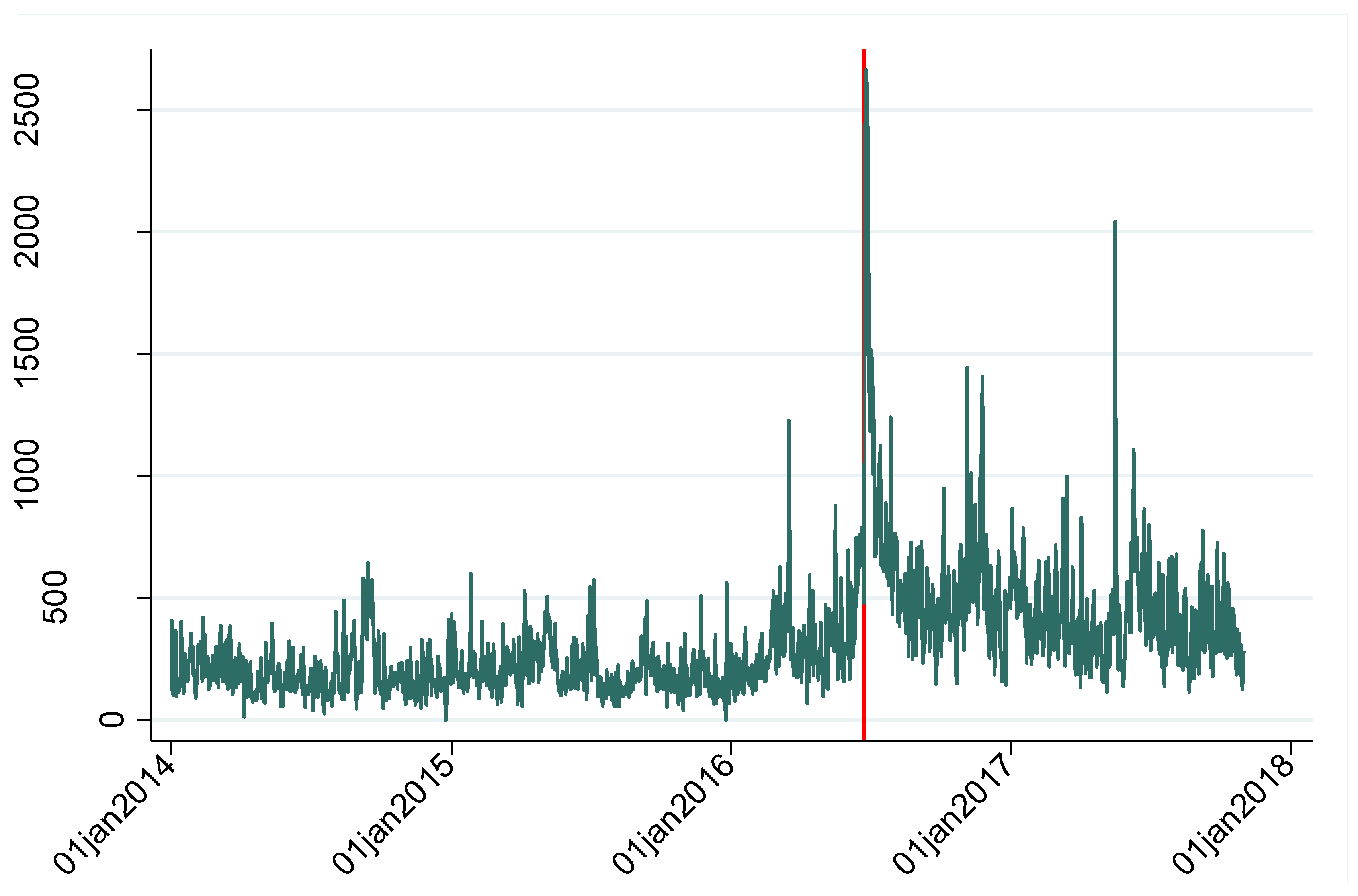
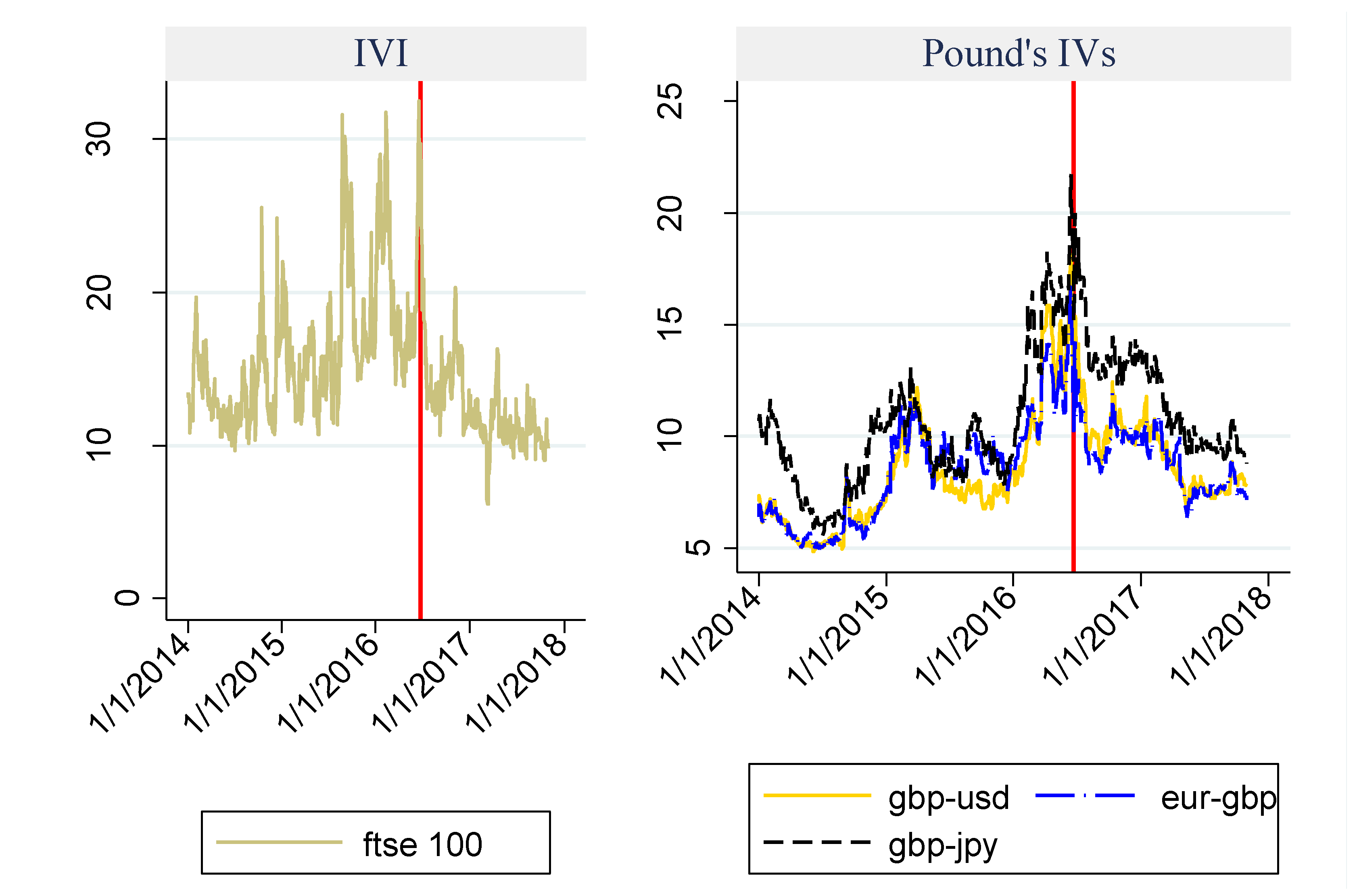
Figure 1 shows the four series under analysis, the vertical bar corresponding to the date of the Brexit referendum (23 June 2016). Starting from mid-2015, the IVI has peaked three times. The last peak coincides with the referendum, after which the IVI has followed a downward trend. In comparison, the GBP-USD IV, EUR-GBP IV and GBP-JPY IV all display wider fluctuations, both before and after the Brexit referendum. Moreover, in the second subsample both GBP-USD IV and EUR-GBP IV have reached much higher levels relative to those observed until the end of 2015; the increase in the case of GBP-JPY IV is much less pronounced, which points to the possibility that “fear” is not equally important for the three exchange rates analysed.

Overall, visual inspection of the data suggests that financial market participants have shown long-lasting eagerness to buy protection against movements in the value of the British pound, whilst concerns about the effects of Brexit on the 100 most highly capitalised companies of the London Stock Exchange may have faded over time. Indeed, the movements of the IVI before and after the referendum are consistent with stock market participants acting in anticipation of the referendum and eventually realising that the major listed companies make most of their revenues outside the UK, and therefore there are fewer reasons to be concerned.

The British pound depreciated sharply on 23 June 2016, falling against the US dollar (from 1.49 to 1.37), the euro (from 1.31 to 1.23) and the yen (from 157.6 to 139.4). In all the three cases, the depreciation continued throughout the remaining months of 2016. Although this protracted depreciation may have been beneficial for the profits of British firms with a global outreach, it is also a sign of what many commentators have remarked—that is, the Brexit shock has mainly been due to political uncertainty (e.g., Baker et al. 2016b) given the prospect of considerably long negotiations with a doubtful outcome (Philippon 2016). Figure 2 shows the behaviour of the UK Economic Policy Uncertainty (EPU) Daily Index, which has a spike on 23 June 2016 and has remained above its pre-2016 level thereafter. In other words, Figure 1 and Figure 2 show that the British pound’s IVs have generally been high since the Brexit referendum, consistently with the high degree of policy uncertainty, whilst the IVI has persistently declined over the same period. In what follows, we test formally whether these patterns (a declining IVI and high IVs) are associated with statistically significant changes in the degree of persistence of each of the series examined.

3. Econometric Analysis

3.1. Methodology

The fractional integration methods used in this paper have the advantage of being more general and flexible than those based on the classical dichotomy between I(0) stationary (e.g., ARMA—autoregressive moving average—models) and I(1) nonstationary (e.g., ARIMA models) series. Allowing for fractional degrees of differentiation provides more reliable information on the effects of the shocks affecting the series, which are transitory if the order of integration is strictly smaller than 1. More specifically, a process {x_t, t = 0, ±1,…} is said to be integrated of order d, and described as x_t ≈ I(d), if it can be represented as:

$${(1-L)}^d{x}_t=u_t,t=0,\pm 1,\dots$$

(1)

where L is the lag-operator (Lx_t = x_t-1) and u_t is I(0), which is defined for our purposes as a covariance-stationary process with a spectral density function that is positive and finite. Moreover, x_t = 0 for t ≤ 0, and d > 0. Note that if u_t in (1) is an ARMA(p, q) process, x_t becomes an AutoRegressive Fractionally Integrated Moving Average (ARFIMA (p, d, q)) process, where d = 0 refers to the stationary I(0) ARMA case, and d = 1 corresponds to the standard ARIMA(p, 1, q) model. Thus, estimating d along with the ARMA components allows for a richer degree of flexibility in the dynamic specification of the data.

In this context, the fractional differencing parameter d plays a crucial role. If d = 0, x_t is said to exhibit short memory or to be I(0) with the effects of shocks disappearing relatively fast, in contrast to the case of long memory that occurs if d > 0. Also, it is important to distinguish between d < 0.5 and d ≥ 0.5, since in the former case the series is still covariance stationary, whilst in the latter the variance increases with the values of d. Finally, if d < 1, the series is mean-reverting and the effects of shocks disappear in the long run, while d ≥ 1 implies a lack of mean reversion. The estimation of d is carried out below implementing both parametric and semi-parametric methods (and using the Whittle function in the frequency domain). Both approaches have pros and cons. The former yields more accurate estimates of d under the appropriate specification; however, in the event of misspecification these are likely to be inconsistent. In this respect, a semi-parametric approach, which does not impose a functional form on the error term, might be preferable.

3.2. Empirical Results

As a first step, we estimate the following model over the full sample:

$$y_t=\alpha +\beta t+x_t,{(1-L)}^d{x}_t=u_t,t=1,2,\dots$$

(2)

where y_t is the series of interest, α and β are unknown parameters to be estimated (corresponding respectively to the intercept and a linear time trend), and x_t is assumed to be I(d), where d is the differencing parameter. Initially, we apply a parametric method, and assume that the errors u_t in (1) are uncorrelated (white noise) and autocorrelated in turn, using the Whittle function in the frequency domain (Dahlhaus 1989; Robinson 1994). In the case of autocorrelated errors, we employ a non-parametric method proposed by Bloomfield (1973) that is well suited to approximating highly parameterised AR(MA) processes with very few parameters within I(d) contexts (see Gil-Alana 2004). The model in (1) is estimated for the three cases of (i) no deterministic terms, (ii) an intercept, and (iii) an intercept with a linear time trend. The results in

Table 1. Estimates of d for the whole sample based on parametric approaches.

(i) No Autocorrelation
Variable	No Regressors	An Intercept	A Linear Time Trend
IVI	0.88 (0.83, 0.93)	0.87 (0.82, 0.92)	0.87 (0.82, 0.92)
USD-GBP IV	1.00 (0.95, 1.05)	1.00 (0.97, 1.05)	1.00 (0.97, 1.05)
EUR-GBP IV	0.97 (0.92, 1.02)	0.95 (0.90, 1.01)	0.95 (0.90, 1.01)
GBP-JPY IV	0.97 (0.92, 1.02)	0.96 (0.92, 1.02)	0.96 (0.92, 1.02)
(ii) With Autocorrelation
Variable	No Regressors	An Intercept	A Linear Time Trend
IVI	0.82 (0.75, 0.91)	0.80 (0.72, 0.90)	0.80 (0.72, 0.90)
USD-GBP IV	0.92 (0.86, 1.01)	0.95 (0.87, 1.04)	0.95 (0.87, 1.04)
EUR-GBP IV	0.89 (0.81, 0.98)	0.86 (0.80, 0.94)	0.86 (0.80, 0.94)
GBP-JPY IV	0.89 (0.83, 0.97)	0.87 (0.82, 0.94)	0.87 (0.82, 0.94)

In red evidence of mean reversion.

indicate that the time trend is not significant in any case, the intercept being sufficient to describe the deterministic component of the series. There is also evidence of mean reversion in some cases, namely for IVI (with both autocorrelated and uncorrelated disturbances), as well as EUR-GBP IV and GBP-JPY IV with autocorrelated disturbances, although the estimated values of d are relatively high in all cases.

Given the different parametric estimates obtained in the two cases of uncorrelated and autocorrelated errors respectively, next we apply a semi-parametric method (Robinson 1995) that does not require any assumptions on the behaviour of the error term. The results are displayed in

Table 2. Estimates of d for the whole sample using semi-parametric approaches.

Variable	IVI	IV USD-GBP	IV EUR-GBP	IV JPY-GBP
25	0.510	0.955	0.848	0.996
26	0.528	0.949	0.837	0.995
27	0.554	0.955	0.830	1.000
28	0.562	0.977	0.844	1.022
29	0.575	0.963	0.824	1.012
30	0.591	0.944	0.818	1.023
31	0.620	0.965	0.835	1.041
32	0.607	0.975	0.849	1.043
33	0.607	0.992	0.865	1.047
34	0.607	0.976	0.850	1.014
35	0.631	0.964	0.854	1.012

In red, evidence of mean reversion. In bold, evidence of unit roots.

, which shows the estimated values for a selected group of bandwidth parameters, m = 25, … (1), … (35), the results being very sensitive to the chosen bandwidth. Here there is evidence of mean reversion in the case of IVI as well as EUR-GBP IV for some bandwidth parameters; for GBP-USD IV and GBP-JPY IV the estimated value of d is not statistically significantly different from 1.

Finally, we re-estimated the model over two subsamples, before and after the Brexit referendum of 23 June 2016, again using both parametric and semi-parametric methods. The break date could also have been determined endogenously. In particular, we find that the Bai and Perron (2003) approach suggests that it should be 15 June 2016, whilst the method of Gil-Alana (2008), specifically designed for the case of fractional integration, points to 17 June 2016 (these test results are not reported for the sake of brevity). Both are very close to the actual date of the referendum, which all considered we decided was the most appropriate to split the sample.

Table 3. Estimates of d for the subsamples before and after the Brexit referendum based on parametric approaches.

(i) No Autocorrelation
Variable	No Regressors	An Intercept	A Linear Time Trend
IVI before	0.86 (0.80, 0.93)	0.85 (0.79, 0.92)	0.85 (0.79, 0.92)
IVI after	0.94 (0.88, 1.02)	0.92 (0.84, 1.00)	0.92 (0.84, 1.00)
USD-GBP IV before	0.93 (0.88, 0.99)	1.11 (1.03, 1.20)	1.11 (1.03, 1.20)
USD-GBP IV after	0.95 (0.88, 1.04)	1.03 (0.95, 1.12)	1.03 (0.95, 1.12)
EUR-GBP IV before	0.93 (0.87, 1.00)	1.11 (1.03, 1.20)	1.11 (1.03, 1.20)
EUR-GBP IV after	0.92 (0.85, 1.01)	0.97 (0.90, 1.07)	0.97 (0.90, 1.07)
GBP-JPY IV before	0.90 (0.86, 0.95)	1.06 (0.99, 1.15)	1.06 (0.99, 1.15)
GBP-JPY IV after	0.96 (0.89, 1.06)	0.94 (0.85, 1.04)	0.94 (0.87, 1.04)
(ii) With Autocorrelation
Variable	No Regressors	An Intercept	A Linear Time Trend
IVI before	0.80 (0.68, 0.91)	0.78 (0.66, 0.91)	0.78 (0.66, 0.91)
IVI after	0.87 (0.76, 0.99)	0.83 (0.72, 1.01)	0.83 (0.71, 0.98)
USD-GBP IV before	0.94 (0.86, 1.07)	0.91 (0.82, 1.04)	0.90 (0.82, 1.04)
USD-GBP IV after	0.84 (0.74, 0.95)	0.91 (0.75, 1.08)	0.93 (0.81, 1.08)
EUR-GBP IV before	0.86 (0.78, 0.97)	0.89 (0.78, 1.06)	0.90 (0.78, 1.06)
EUR-GBP IV after	0.80 (0.71, 0.92)	0.87 (0.69, 1.05)	0.90 (0.77, 1.06)
GBP-JPY IV before	0.94 (0.88, 1.03)	0.90 (0.83, 1.02)	0.90 (0.82, 1.03)
GBP-JPY IV after	0.84 (0.74, 0.95)	0.62 (0.50, 0.87)	0.79 (0.68, 0.90)

displays the parametric results, distinguishing between the cases of uncorrelated (Table 3i) and autocorrelated (Table 3ii) disturbances. In the latter case the estimated value of d for IVI increases from 0.85 (which implies mean reversion) to 0.92 (suggesting a lack of mean reversion since the unit root hypothesis cannot be rejected). By contrast, the decrease in the degree of persistence observed for the IVs after the break is not statistically significant. When allowing for autocorrelated disturbances, the estimated value of d for IVI increases (from 0.78 to 0.83), and the same holds for GBP-USD IV and EUR-GBP IV.

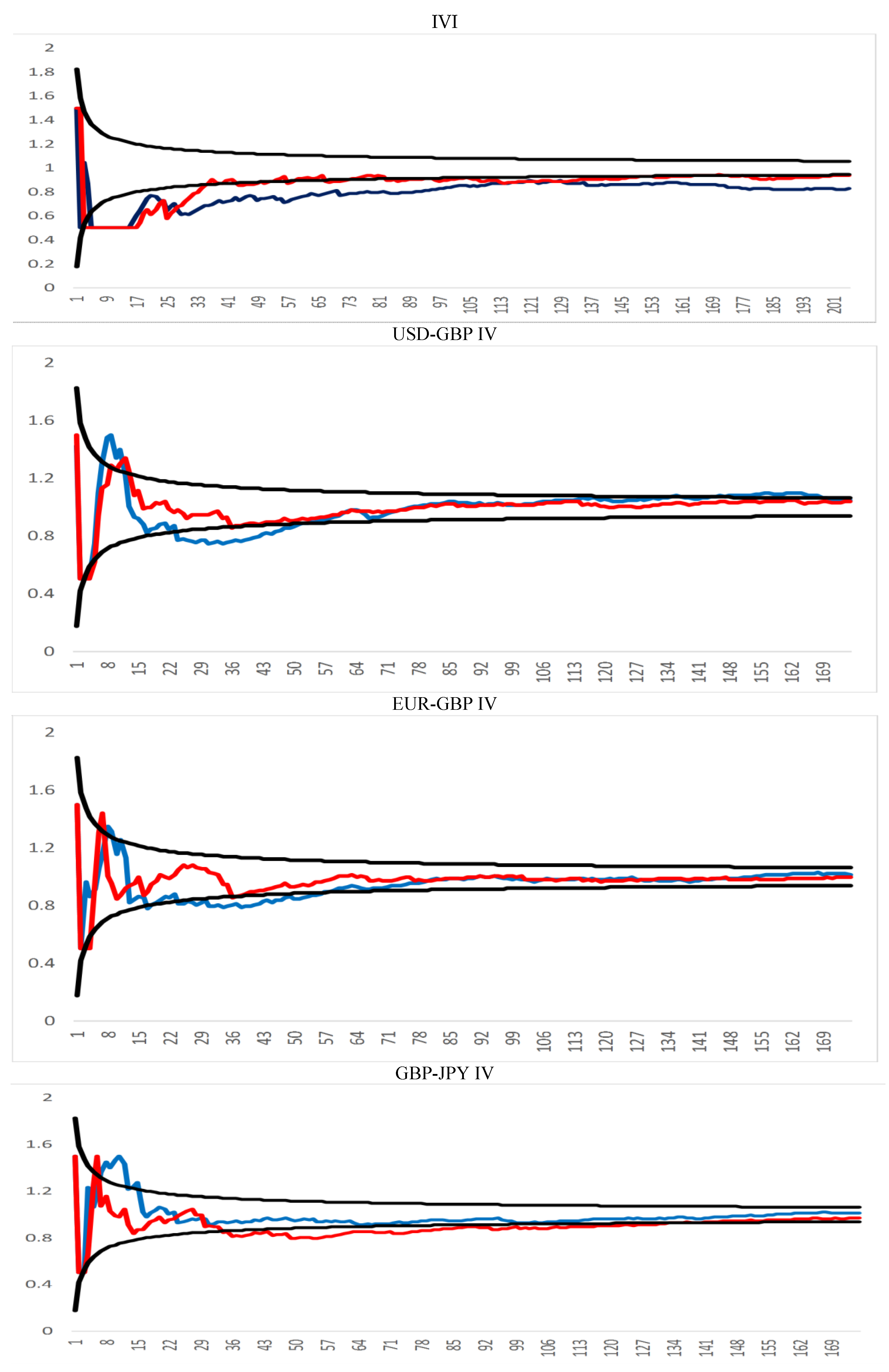
The semi-parametric estimates of d, before and after the break, are displayed in Figure 3 for all the possible bandwidth parameters. Consistently with the parametric results, the evidence suggests an increase in the degree of persistence after the Brexit referendum for IVI, GBP-USD IV and EUR-GBP IV, but not for GBP-JPY IV. In other words, it seems that the referendum created a new economic environment in which shocks have more long-lasting effects on market sentiment and investor fear than previously. This suggests that the UK government should act swiftly to complete the negotiations with the EU, agreeing on the terms and conditions of Brexit in order to remove the existing (political) uncertainty. At present concerns about economic growth and financial trading undoubtedly are playing a role, and a well-structured Brexit deal would lessen if not eliminate them.

Whether the change in persistence detected by our methodology is driven exclusively by the uncertainty associated with Brexit or there are other concurrent factors remains an open question, which is outside the scope of this paper. Our objective here has been to examine the size and statistical significance of changes in the behaviour of financial indicators of market fear around the date of the referendum. Our analysis provides evidence consistent with patterns already spotted by both economists and policymakers (e.g., Baker et al. 2016b; Kierzenkowski et al. 2016; Philippon 2016). Future work will include in the model control variables to take into account explicitly other factors. However, it seems extremely plausible that the significant change in the behaviour of the IVI and the British pound’s implied volatilities that we have documented is mainly due to the Brexit referendum; it is unlikely that such a sudden and significant shift could have been driven by other economic or policy developments.

4. Conclusions

This paper examines the effects of Brexit on uncertainty in European financial markets. More specifically, it applies (parametric and semi-parametric) fractional integration methods to test for any changes of the degree of persistence of the FTSE 100 Implied Volatility Index (IVI) and of the British pound’s implied volatilities (IVs) vis-à-vis the main currencies traded in the FOREX, namely the euro, the US dollar and the Japanese yen.

Visual inspection of the data covering the period from the beginning of 2014 to the end of October 2017 suggests that the IVI reacted in anticipation of the Brexit referendum and has been declining thereafter, whilst the British pound’s IVs have remained above their initial level since the referendum. This evidence is consistent with the fact that British firms with global outreach are in a better position to manage the risk implied by the Brexit negotiations. On the other end, market participants seem to feel the need to continue buying protection against future swings in the British pound.

The econometric analysis provides evidence of a significant increase in the persistence of all the series considered except the GBP-JPY IV, which indicates that Brexit has had a noticeable impact (at least in the short run) on uncertainty. Since the IVI and the British pound’s IVs can be interpreted as “investor fear gauge” (see Whaley 2000), it seems clear that investors have taken a dim view of the consequences of Brexit, especially because of the prolonged political uncertainty associated with this process and its uncertain future outcome, the “fear” factor becoming more persistent as well as more sizeable in most cases and affecting investment strategies. Although it is too early to express a view on the long-term effects of Brexit (especially on the real economy) there has been a short-term negative impact on financial markets; achieving an appropriate Brexit deal in the near future appears to be of paramount importance for the British economy. Future work will extend the analysis to consider other factors that might have affected market sentiment.