A Logistic Regression Based Auto Insurance Rate-Making Model Designed for the Insurance Rate Reform

Abstract

Using a generalized linear model to determine the claim frequency of auto insurance is a key ingredient in non-life insurance research. Among auto insurance rate-making models, there are very few considering auto types. Therefore, in this paper we are proposing a model that takes auto types into account by making an innovative use of the auto burden index. Based on this model and data from a Chinese insurance company, we built a clustering model that classifies auto insurance rates into three risk levels. The claim frequency and the claim costs are fitted to select a better loss distribution. Then the Logistic Regression model is employed to fit the claim frequency, with the auto burden index considered. Three key findings can be concluded from our study. First, more than 80% of the autos with an auto burden index of 20 or higher belong to the highest risk level. Secondly, the claim frequency is better fitted using the Poisson distribution, however the claim cost is better fitted using the Gamma distribution. Lastly, based on the AIC criterion, the claim frequency is more adequately represented by models that consider the auto burden index than those do not. It is believed that insurance policy recommendations that are based on Generalized linear models (GLM) can benefit from our findings.

1. Introduction

As of 2016, the amount of total property insurance premiums continues to increase, which makes total property insurance the biggest part in the property insurance industry.

At present, the international approaches of rate making are mainly chauvinism and humanitarianism. Traditional Chinese insurance companies are mainly from chauvinism, which is the value of the car itself. However, with the development of the insurance industry, the existing provisions begin to consider human factors, including driving record, driver’s age, family members, regional factors and so on. This is more conducive to the mobilization of the driver’s initiative, making the burden of insurance premium more reasonable.

China market reform of auto insurance rate has been a few twists and turns. On 1 June 2015, as one of the six pilot areas for deepening the reform of the auto insurance rate management system in China, Chongqing officially started the commercial terms for the reform of the auto insurance rate management system.

The main content of the rate reform is that after adjustment, a total of four rate adjustment coefficients under the new tariff system are determined, including bonus-malus coefficient (NCD), independent channels coefficient, autonomous underwriting coefficient, the traffic law coefficient and the client discount coefficient. Especially the independent channels coefficient and autonomous underwriting coefficient are the embodiment of pricing power for the insurance companies to choose. After the reform, the risk of financial insurance companies expanded, putting forward higher requirements for the management strategy of insurance companies.

Therefore, it is of great significance to discuss the reform of auto insurance rates. According to the regulations of the new reform, auto burden index will be introduced to quantify the model analysis. And the auto insurance rate-making is studied on the basis of practical data. Firstly, cluster analysis was used to classify the risk categories into three kinds of risk categories according to the age of owners, vehicle age and vehicle burden index. After the reform, the insurance company may set different business car insurance rates, according to their own risk recognition, risk cost and risk pricing power, motor vehicles and drivers of different risk levels. The improvement of the pricing power of insurance companies and the increase of consumers’ satisfaction have confirmed the initial success of the commercial car insurance reform.

The paper is organized as follows. In Section 2, the data and the auto burden index are introduced. The results of the cluster analysis are discussed in Section 3. In Section 4, the selection procedure of the loss distribution is presented and the preferred distributions for both claim frequency and claim cost are given. In Section 5, the claim frequency is fitted by logistic regression model considering the auto burden index. A conclusion for our proposed method is drawn in Section 6.

2. International Research Background

Risk classification plays a part to eliminate cross-subsidy between people with low and high risks, which contributes to promote the market efficiency, as well as the increase of social risk cost and the loss of fairness. The impact on equity and efficiency in the insurance market has always been the focus of debate. The first study of the risk classification is Hoy (1982), the R-S equilibrium, Wilson equilibrium and Miyazaki’s assumption are expected as the underwriter contracts in the cross-subsidy equilibrium model, the results showed that the causal relationship between risk classification and economic efficiency is not clear, which depends on the classification and form of equilibrium. Crocker and Snow (1986) made more detailed studies, they did not categorize the groups in the utility of boundary classification, otherwise, they came to the following conclusions. First, any market equilibrium with no cost classification is better than that of without classification. Second, it is not easy to measure fairness and efficiency of resource costs according to classification and it may be effective to ban some sort of cost classification. Lereah (1983) and Cheng (2007) compared the effects of different risk classification subjects. They believed that there are two options for insurance companies to classify the insured, one is that the insurance company is independent and the other is the risk assessment institution. The two schemes differ in cost and accuracy. The risks in auto insurance were classified by cluster analysis in this paper. Since the beginning of the 20th century, some scholars have studied non-life actuarial models. The classification rate, general rate and individual risk rate are the main non-life insurance pricing methods. Among them, classification rate is a kind of non-life insurance pricing method based on risk classification, which has a certain universality and is not lack of pertinence to specific groups. Finger (2001) of this method has carried on the detailed narration, more scientifically expounds the classification rate set: the basic idea of the large number of individuals with homogeneous risk is divided into the same category, through the statistical method to determine the relative abundance of each group level and the corresponding parameters and then get the group rate. In 1960, Bailey and Simon (1960) believed that the basis of classification rates was to group individuals of the same risk characteristics, determine the relative number of risk levels of each group and then calculate relative rates. Bailey (1963) presented a single analysis method to study the impact factors of single rate on policy prices. On this basis, Holler et al. (1999) summed up to determine the level of the relative abundance of three basic methods, namely the minimum deviation method, maximum likelihood method and loss relative ratio method, at the same time points out the defects of various methods.

Generalized linear model (GLM) is the earliest by Nelder and Wedderburn (1972) put forward and give a specific definition, in the aftermath, Anderson et al. (2004) of the generalized linear model of exponential distribution density function and the form of moment generating function are discussed and the specific distribution types of exponential distribution family, such as the gamma distribution, poisson distribution is introduced in detail. McCullagh et al. first applied GLM to the actuarial field. Since then, GLM has been widely used in non-life insurance rates and has become a standard method for auto insurance rates. However, with the development of actuarial theory and the practice of premium rate making accuracy requirement for further improve, GLM also exposed some defects in the application, therefore scholars on the many kinds of extension. Pregibon et al. (1984) proposed a dual generalized linear model (DGLM) that established the model of the mean and divergence parameters of the reaction variables and extended the traditional generalized linear model further. Smyth introduces the maximum likelihood estimation of DGLM and considers the situation of normal and inverse Gaussian distribution. Smyth applies DGLM to non-life insurance pricing and forecasts the rate of vehicle loss but excludes regional factors in empirical research and the rate structure is not reflected in regional differences. In terms of application of premium rate making model, Aitkin et al. (1989) studied a lot of application examples of generalized linear models, including the poisson distribution is used to simulate insurance claims data for multiple vector list in the distribution of cell count Ohlsson and Johansson (2010) introduced the generalized linear model in the practical application in automobile insurance, through empirical analysis, data selection for claim frequency poisson distribution model, to choose a claim intensity gamma distribution model in fitting, gives a detailed introduction and rigorous derivation.

3. Data

After the reform of auto insurance rate system in China, 2015, the insurance companies determined auto insurance rates for autos and drivers with different risk levels, considering the factors including risk identification capabilities, risk costs, risk pricing capabilities. Based on the new regulations of the reform, we used the data of an insurance company in Chongqing, China, with a total of 33,373 sets of insurance policies, ensuring the authenticity and effectiveness in the analysis. While Adriana Bruscato Bortoluzzo (2011) classified the auto types into luxury, medium and small with an index respectively. In this article, we introduce the auto burden index into the model to precisely quantify the auto types, transforming the auto types into specific values, which is described by the formula,

Single commonly used accessories price × accessories loss rate ÷ auto sales price × 100

The insurance policy mainly includes claims frequency last year, license plate numbers, auto age, owners’ age and the settled claims. The auto burden index in this article was jointly issued by China Insurance Industry Association and China Automobile Maintenance Industry Association, with a total of 526 auto burden indexes of the commonly used auto types. After removing the insurance policies with undefined auto burden index or missing data, the remained 2783 sets of insurance policies were used as experimental data.

The Statistical Verification of the Auto Burden Index

The higher the burden index, the higher the claim amount. The higher the index, the better the overall performance of the auto is and the lower the accident rate is. Consequently, the claims frequency is negatively correlated with the auto burden index. The latter part of the empirical test also validates this view. The overall significance function of the model is

$$p=E(y=1|x_1,x_2,\cdots ,x_r)=\frac{e^{{\beta }_0+{\beta }_1{x}_1+\cdots {\beta }_r{x}_r}}{1+e^{{\beta }_0+{\beta }_1{x}_1+\cdots {\beta }_r{x}_r}}$$

The function is an incremental function, the auto burden index and the claim frequency is negatively correlated. The decrease of p value indicating an increase in the model significance.

4. Classification of Risks—Cluster Analysis

Risk classification refers to that the insurer can distinguish between high-risk and low-risk policyholders based on the variables containing the risk information of policyholders. If high-risk and low-risk policyholders can be completely distinguished, it is called complete classification. Otherwise, if there are a small number of low-risk policyholders in the high-risk group after the risk classification, or a small number of high-risk policyholders in the low-risk group, it is called incomplete classification.

In the auto insurance business, it is necessary to assess the risk of the policy amount and classify the risks of the insured, which are called the classification rates. The selected risk determinants are also called rate factors. Cluster analysis is an unsupervised learning process for finding similar sets of elements in a data set. The common feature of this method is that when the number and structure of the classes are unknown, the similarity between these data is measured by a certain distance criterion. The information of the insured (age, gender, etc.), the information of the auto (auto type, age, etc.), the claim frequency and the settled claim are in close connection with each other, it’s important to find out their relations in the classification. In this article, the information of the insured is clustered and different characteristics of types are obtained and the decision support is provided to the insurance company through the analysis. x_ij represents a latent variable by the candidate in sample i and indicator j, each sample has p variables, we selected six variables for each sample, including the ‘total signed premium,’ ‘owners age,’ ‘the claim frequency last year,’ ‘settled claim,’ ‘the auto burden index’ and ‘auto age.’ We use x_j and r_i to denote the variable j and the sample i respectively, d_ij is used to express the distance between sample i and the sample j. Comparing with the common distances, it’s easy to find out that the real data is better fitted with the European distances, which is described by formula as:

$$d_{ij}=\sqrt{{\displaystyle \sum _{k=1}^p{(x_{ik}-x_{jk})}^2}}$$

Regarding each sample as a separate class, the basic ideas of system cluster are as follows: first specify the distances between samples and the distances between classes, secondly merge the nearest two classes into a new class, then calculate the distance between the new classes and the other classes, repeating the merger of the nearest two classes until all the samples are merged into one class. d_ij represents the distance between the sample i and the sample j, G₁ and G₂ represent classes and D_KL represents the distance between the class K and the class L. The Ward method is used to system cluster in this article. Based on the idea of variance analysis, if the classification is correct, the sum of squares between the same classes should be small, the sum of squares between different classes should be large. The number of samples in this paper is large, the two classes tend to have a relatively large distance, so we choose the Ward. Suppose G_K and G_L are merged into a new class, the sum of squares of G_K, G_L and G_M are as follows:

$$\begin{array}{l}{W}_K={{\displaystyle \sum _{i\in G_K}(x_{(i)}-\overline{x_K})}}^T(x_{(i)}-\overline{x_K})\\ W_L={{\displaystyle \sum _{i\in G_L}(x_{(i)}-\overline{x_L})}}^T(x_{(i)}-\overline{x_L})\\ W_M={{\displaystyle \sum _{i\in G_M}(x_{(i)}-\overline{x_M})}}^T(x_{(i)}-\overline{x_M})\end{array}$$

The above formulas reflect the dispersion degree of the samples in each class and the sum of squares between G_K and G_L is:

D_KL2 = W_M − W_K − W_L

In this section, the data is clustered by R software and the 2783 sets of data are divided into three classes, 1–536 for the first class and 537–1760 for the second class, the remaining as the third category.

4.1. The Distribution of the Total Signed Premium and the Settled Amount

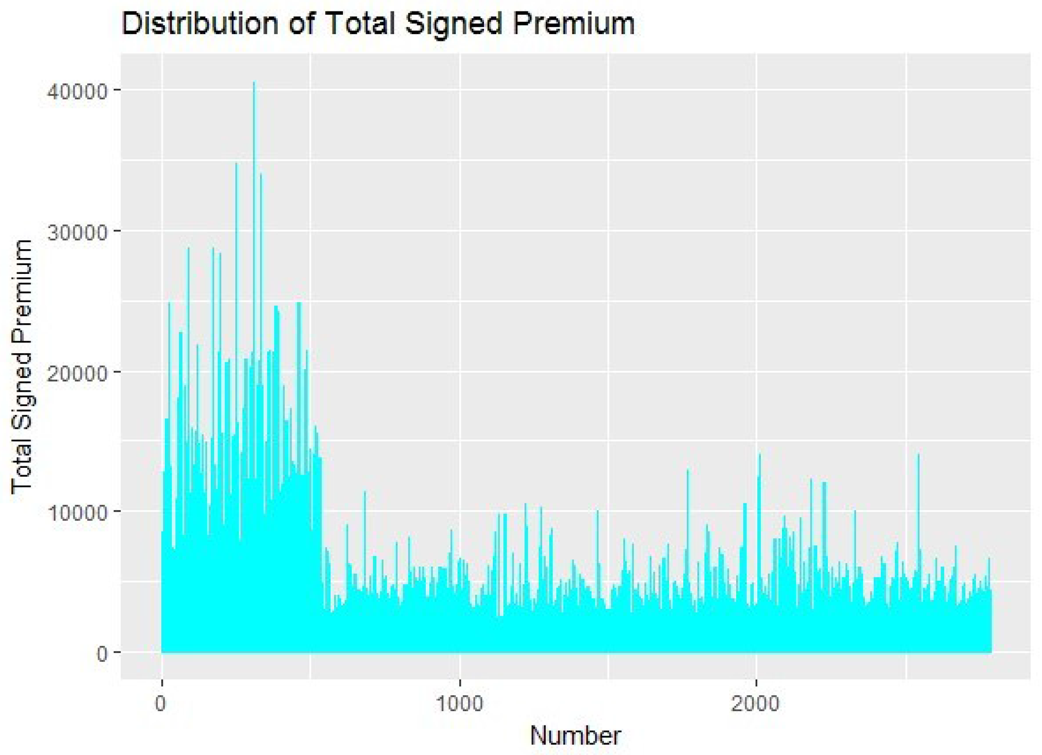
After clustering, the total signed premium is classified into the three classes, as shown in Figure 1.

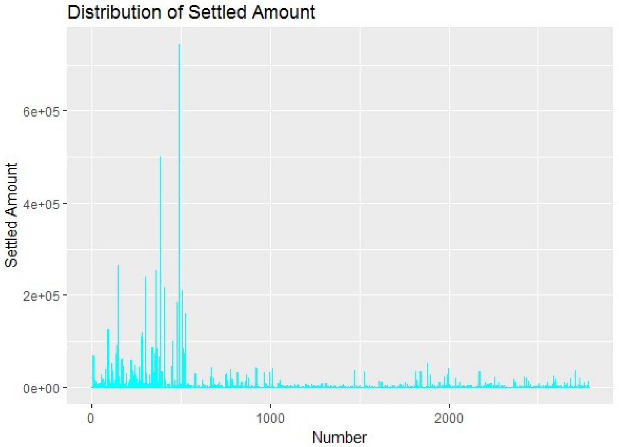
Since the raw data is provided by the insurance company with better practical significance on the market, we can see that the total signed premium of the first class 1–536 is much higher than the other two classes. Therefore, the first class should be regarded as a high-risk class, which requires a higher premium. The second class 537–1760 should be regarded as a low-risk class, which requires a lower premium. The total signed premium of the third class 1761–2783 is smaller than the first class but the volatility is greater than the second class, so that the second class can be regarded as uncertain risk class, which requires being discussed further. The settled amount is the cumulative compensation amount of a case that has been filed and closed, which plays an important role in the operating income of the insurance company, including the cumulative compensation amount of payment that has been closed and paid out of or has been closed and unpaid. The settled amount is classified according to the clustering result, as shown in Figure 2.

According to Figure 2, the distribution of the settled amount is consistent with the distribution of the total signed premium. Therefore, it can be generally considered that the first class should be regarded as a high-risk class, the second and the third class still need further analysis. According to the above classification results, we will further discuss the classification of variables.

4.2. Analysis of the Variable Classification

4.2.1. Burden Index

According to the classification of the auto burden index, the results as shown in

Table 1. Distribution of the auto burden index.

Burden Index	0–10		10–20		20–30		Above 30
	Number	Proportion	Number	Proportion	Number	Proportion	Number	Proportion
The first class	44	8.21%	307	57.28%	168	31.34%	17	3.17%
The second class	279	22.79%	912	74.51%	33	2.70%	0	0.00%
The third class	259	25.30%	761	74.31%	4	0.39%	0	0.00%

.

Compared with the second and third categories, the first group of the burden of more than 20 people accounted for the highest proportion, that is, the first category of high risk category. In the first category, more than 20 people accounted for the highest proportion, or 81.9% of the vehicles belonging to the first category of high-risk category.

The second and the third class both hold the highest proportion in the auto burden index between 10 and 20, which can be regarded as a low-risk class or still require further discussion. This is consistent with the distribution of the total signed premium.

4.2.2. Owner’s Age

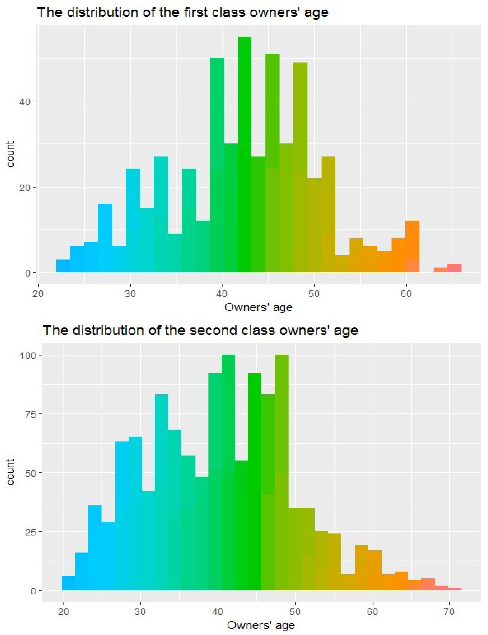
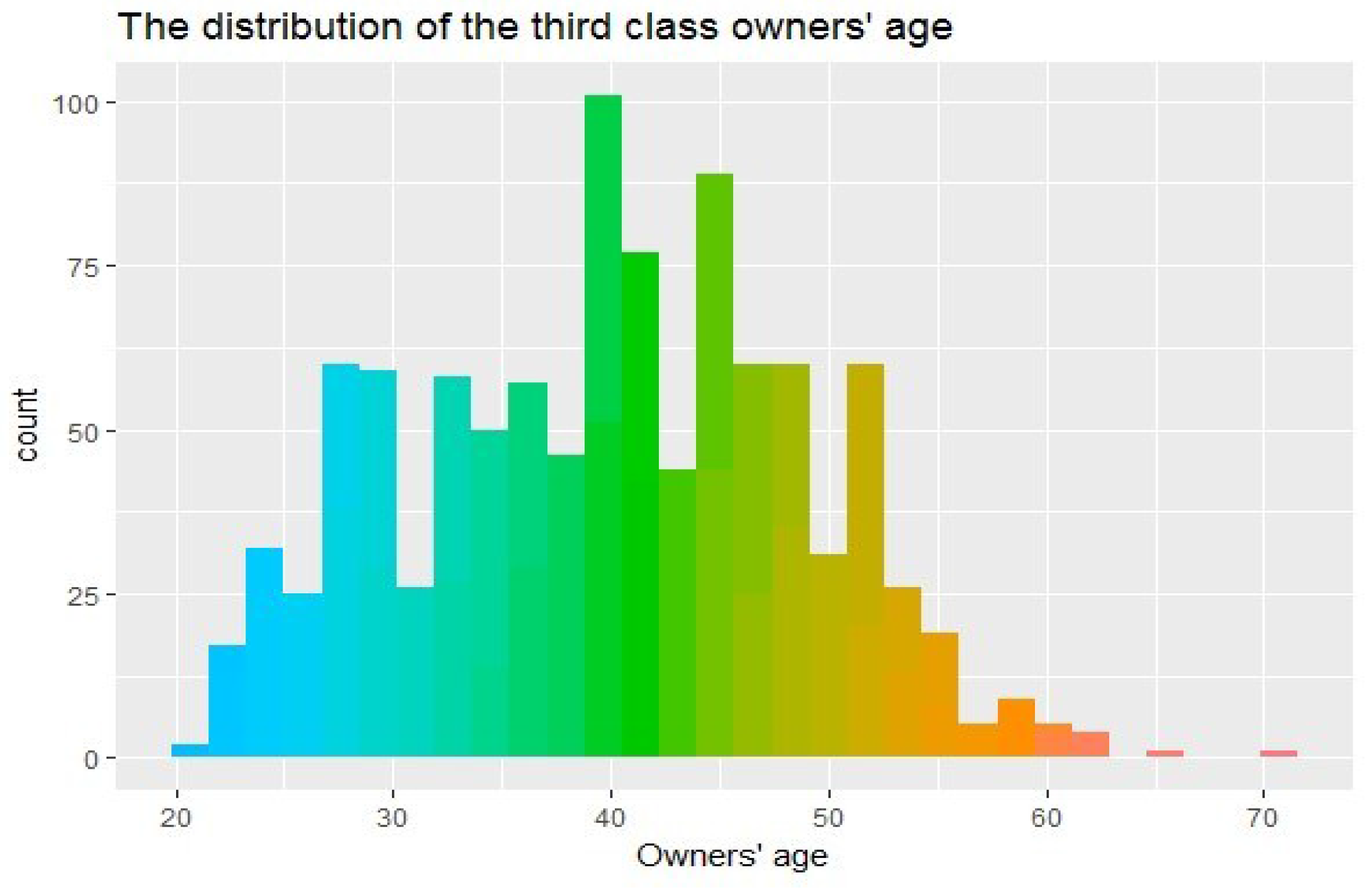
According to the classification of owners’ age, the results are shown in Figure 3.

As shown in Figure 3, the first class of owners’ age is centrally distributed between 39 and 51 years old, the second class is centrally distributed between 25 and 53 years old, the third class is centrally distributed between 23 and 55 years old. In case of the clustering result, there is no significant relationships between the owners’ age and the risk classification. By experience, younger drivers are more likely to have accidents due to lack of driving experiences but drivers of this age group have higher physical quality and relatively high response ability.

4.2.3. Auto Age

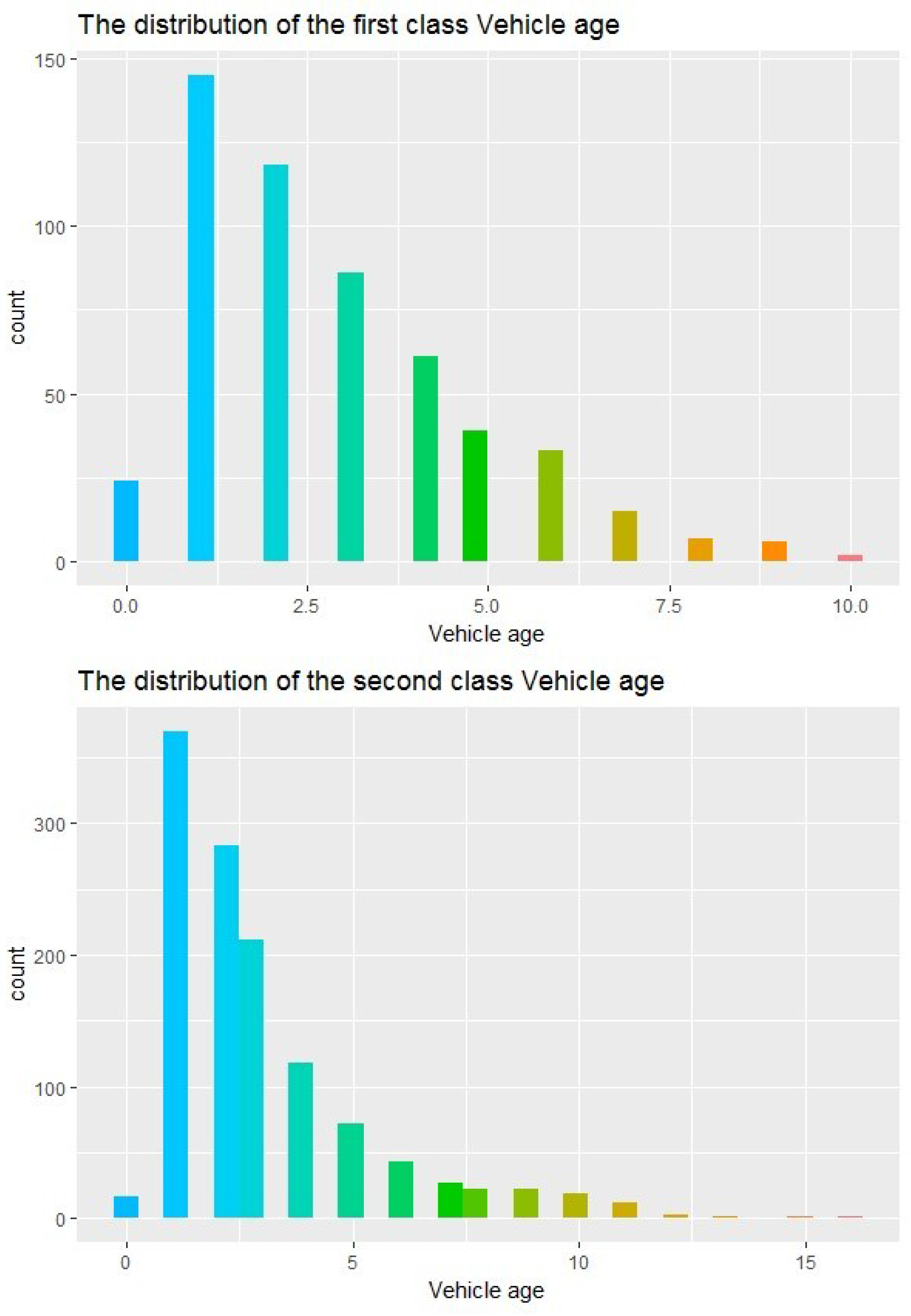
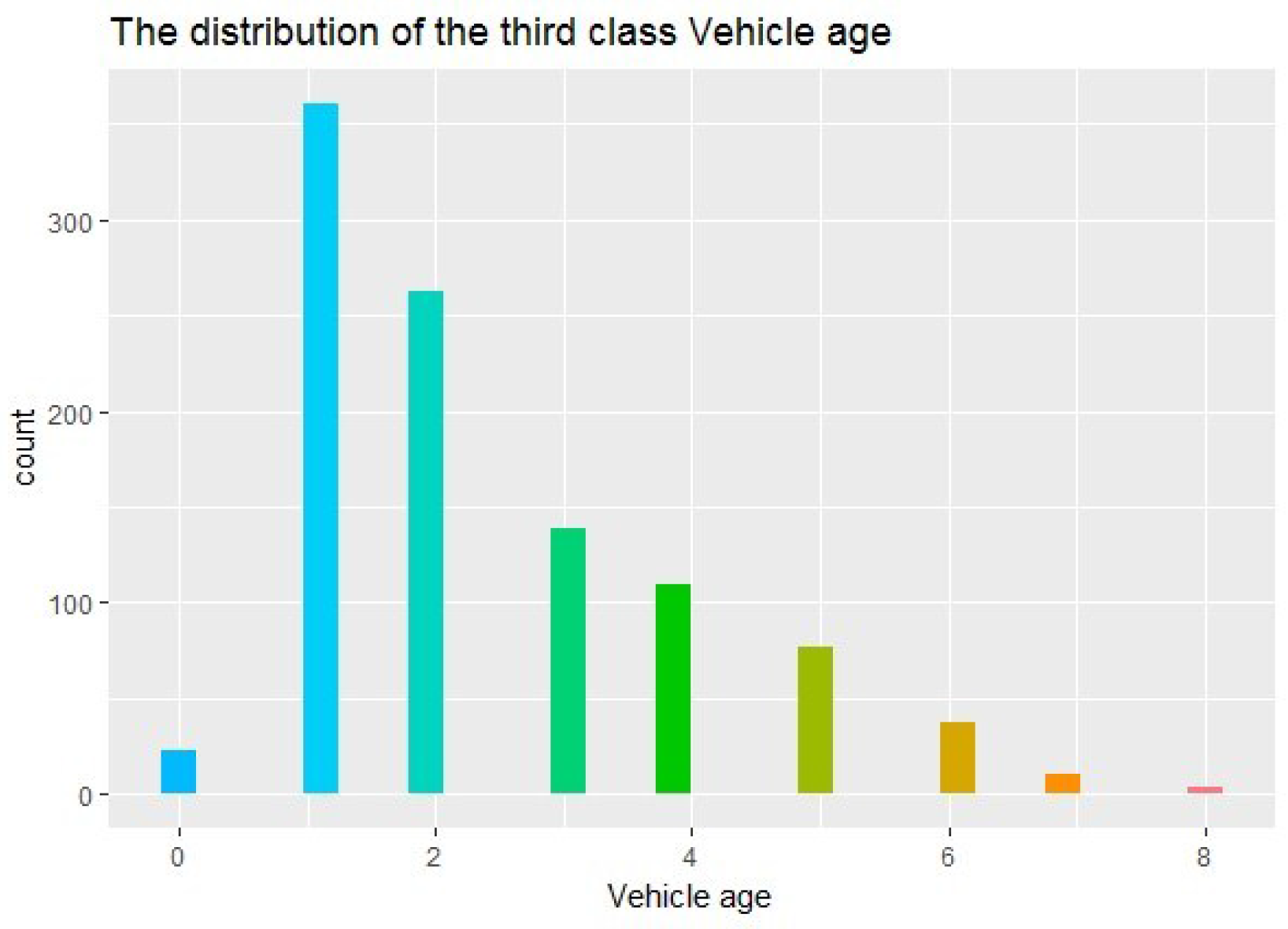
According to the classification of the auto age, the results are shown in

Table 2. Classification of auto age.

Auto Age (Years)	0	1	2	3	4	5	6	7	8	9	10	10 or more
The First Category	24	145	118	86	61	39	33	15	7	6	2	0
The Second Category	17	370	283	212	118	72	43	27	22	22	19	19
The Third Category	23	361	263	139	109	77	37	11	4	0	0	0

and the distribution of auto age is presented in Figure 4.

According to the high-risk definition of the first class, the auto age of the second class is concentrated in 1–3 years but autos that are older than 10 years old are all in this class. The auto ages of the third class are concentrated in 1–3 years old, which means the autos are in a good situation with no elder ones.

Therefore, the determination of the risk based on auto age still needs further validation.

4.2.4. Claim Frequency

According to the classification, the results are shown in

Table 3. Distribution of claim frequency in three classes.

Claims Frequency	−3	−2	−1	1	2	3	4	5
The First Class	31	57	152	271	0	20	3	2
The Second Class	211	212	412	388	0	1	0	0
The Third Class	86	111	284	490	0	40	9	4

.

From Table 3, it can be seen clearly that the claim frequency under 0 in the second and third classes hold a higher proportion, which is consistent with the lower signed premium in the second and third class. The claim frequency under 0 in the first class holds a lower proportion, which is consistent with the higher signed premium in the first class.

4.2.5. The Economic Significance of Variables

The economic significance of variables in the model are as follows:

(1)

There is certain reference value of the auto burden index for the vehicle insurance rate. Through the clustering results, it is suggested that insurance companies could predict the premiums of the insured by introducing the auto burden index into the model. In the empirical study, the autos with a higher burden index ware charged with a relatively high premium. Therefore, insurance companies could divide them into high-risk class, especially the autos with auto burden index more than 20 deserve more attention.

(2)

Based on the clustering results of owners’ age and auto age, it is suggested that the influence of driving experience should be considered in the evaluation of the auto owners by insurance companies. And the auto with a younger age is supposed to have a good condition, which helps to safe driving. However, according to the above results, the influence of auto age on risks should be discussed in more details. Autos with good conditions have a large proportion in the first high-risk class. Studies have shown that most auto accidents are caused by human factors. This view also confirms the clustering results of auto age. However, for autos over 10 years of age, further discussion and analysis are still needed in the insurance process.

(3)

After the reform of commercial auto insurance in Chongqing in 2015, non-claiming benefits will be taken into account in the auto insurance rate, which means that persons with fewer insured in the past are supposed to pay lower premiums. In the first high-risk class, the claims frequency of policyholders is relatively high, along with an increase in the risk, wherefore it is reasonable for the insurance company to charge higher premiums.

5. Selection of the Loss Distribution

It’s difficult to construct the empirical distribution of the insured for quantitative analysis, so that the use of loss distribution is a better alternative, which requires selecting the appropriate distribution among several loss distributions. This section is implemented using the GENMOD program in SAS software. In this article, two different distributions are used to figure out the correlation of claim frequency and variables, claim cost and variables. We use the Poisson distribution and the negative binomial distribution to fit the claim frequency in case it follows a discrete distribution. We use the Gamma distribution and Inverse Gaussian distribution to fit the claim cost in case it follows a continuous distribution. According to the canonical form of the link function, we use the logarithm function, the logit function and the identity function respectively in the Gamma distribution and the Poisson distribution, the negative binomial distribution and the Inverse Gaussian distribution.

The formula of the claims cost is as follows, indicating an opposite relationship between the claim cost and the claim frequency.

$$S=\frac{L}{N}$$

S is the claimscost, L for the losses and N is the claim frequency. The average loss per claim intensity can be based on net loss, excluding various loss-adjusted costs, as well as assessed or total loss-adjusted costs, which can be paid, incurred, or predicted final losses. The claim could be the number of final claims that have been reported, paid, closed or predicted.

5.1. Loss Distribution of Claim Frequency

For non-life insurance business, the distribution of individual insurance claims frequency is uncertain. The claims frequency can be described as a random variable, which can be described by its probability distribution. The theoretical distributions of claims frequency are Poisson distribution, binomial distribution and negative binomial distribution.

The Poisson distribution and the negative Binomial distribution are commonly used to fit the claim frequency since it is a non-negative discrete variable. In the context of actuarial literature, Denuit and Lang (2004), Yip and Yau (2005) and others proposed the extracted reference from the Poisson distribution, which is used as the main method to estimate the claim frequency. The negative binomial distribution is used as a functional form to relax the restriction of equidispersion in the Poisson model. The literature presents many of the ways to construct the negative binomial distribution but Boucher et al. (2008) argue that the more intuitive one is the introduction of a random heterogeneity term of mean 1 and Variance in the mean parameter of the Poisson distribution. This general approach is discussed at length by Winkelmann (2004) and Greene (2008) and so on. Regarding the usage of the insurance data, a classic example arises from the theory of accident proneness which was developed by Greenwood and Yule (1920).This theory sustains that the number of accidents follows the Poisson distribution but there is Gamma-distributed unobserved individual heterogeneity, reflecting the fact that the true mean is not perfectly observed. The distribution function of the Poisson distribution can be expressed as:

$$P_r(Y_i=y_i)=\frac{\exp (-{\lambda }_i){\lambda }_i{}^{y_i}}{y_i!}$$

The probability density function of the negative binomial distribution is:

$$P_r(Y_i=y_i)=\frac{\Gamma (\alpha +y_i)}{\Gamma (\alpha )\Gamma (1+y_i)}{(\frac{\alpha }{\alpha +y_i})}^{\alpha }(\frac{{\lambda }_i}{{\lambda }_i+\alpha })$$

The mean and variance of the negative binomial distribution is E(Y_i) = λ_i and $Var(Y_i)={\lambda }_i+\frac{{({\lambda }_i)}^2}{\alpha }$. According to the relationship between the mean and variance, the negative binomial distribution is the more over-dispersed with a smaller α. When α → ∞, the negative Binomial distribution is degenerated into Poisson distribution. According to the factors of ratemaking used by the China Insurance Industry Association, we made a classification of the owners’ ages, the auto burden index, the driving areas in Chongqing, auto age, the claim frequency and the claim cost, Five levels are divided according to the above indicators, as shown in

Table 4. Rate factor grading table (Yu represents Chongqing in China).

Level Factor	1	2	3	4	5
Owners Age	[20, 30)	[30, 40)	[40, 50)	[50,60)	[60, 70)
Auto burden index	[0, 10)	[10, 15)	[15, 20)	[20, ∞)
Area	Yu A	Yu B	Yu C	Yu F	Yu G
Auto age	[0, 90)	[90, 360)	[360, 1080)	[1080, 1800)	[1800, ∞)
Claim cost	[0, 1)	[1, 3)	[3, 8)	[8, 15)	[15, ∞)

. (unit: thousand).

According to

Table 5. The claim frequency fitted by two distributions.

Factors	Level	Poisson Distribution		Negative Binomial Distribution
		Coefficient	p Value	Coefficient	p Value
Intercept		−6.4953	0.0168	−7.8303	0.0133
Owners age	1	−2.7985	0.0493	−1.6278	0.0701
Owners age	2	−2.4399	0.054	−1.3198	0.0756
Owners age	3	−5.3297	0.0181	−2.6768	0.0528
Owners age	4	−2.5146	0.0543	−1.7192	0.0679
Owners age	5	0.0000		0.0000
Auto burden index	1	−0.2658	0.2074	−0.0747	0.7611
Auto burden index	2	0.1331	0.4598	0.0166	0.9361
Auto burden index	3	0.2362	0.2429	0.0785	0.7361
Auto burden index	4	0.0000		0.0000
Area	1	−0.18	0.3413	−0.0786	0.7167
Area	2	0.0796	0.7105	0.0354	0.8835
Area	3	0.1777	0.3848	0.0616	0.7914
Area	4	0.3751	0.0891	0.1784	0.4749
Area	5	0.0000		0.0000
Auto age(days)	1	−0.2635	0.0339	−0.1023	0.0730
Auto age	2	−0.7033	0.0004	−0.3378	0.1268
Auto age	3	−0.6578	0.0012	−0.3744	0.0957
Auto age	4	−0.6935	0.0006	−0.3980	0.0713
Auto age	5	0.0000		0.0000

, the claim frequency is negatively correlated with the owner’s age and the auto age, the physiological status and psychological state of the auto owners are closely related to their ages. Generally, young people are more aggressive. Although older drivers are more prudent because of their rich driving experience, their physiology will gradually recess as age increases. As a result, older drivers have much slower emergency response than young people, so that both young and old drivers belong to the group with high accident rates. The coefficients of auto burden index and driving areas did not pass the significance test in the two distributions, so that they require to be further analyzed. David and Jemna (2015) fitted the claim frequency with the Poisson distribution and the Negative Binomial distribution respectively, they pointed out that the Negative Binomial distribution fitted claim frequency better than the Poisson distribution. According to the fitting results of the Poisson and negative binomial distributions of the claim frequency, the p-value of the estimated parameters in Poisson distribution is obviously smaller than that of the negative binomial distribution, indicating that the fitting result of Poisson distribution is relatively better. Based on the data in this article, we found that the Poisson distribution has a better fitting effect than the Negative Binomial distribution.

5.2. Loss Distribution of Claim Cost

Since the claim costs usually follow a negatively skewed distribution, they are usually fitted by the Gamma distribution and the Inverse Gaussian distribution. The probability density function of the Gamma distribution can be expressed as:

$$f(y_i)=\frac{1}{y_i\Gamma (v)}{\left(\frac{y_{i}v}{\mu }\right)}^v\exp (-\frac{y_{i}v}{\mu })$$

The probability density function of the Gamma distribution is negatively skewed and its variance equals to the square of the mean. The probability density function of the Inverse Gaussian distribution can be expressed as:

$$f(y_i)=\frac{\lambda }{\sigma \sqrt{2\pi y_i{}^3}}\exp [-\frac{1}{2y_i}{(\frac{y_i-\mu }{\mu \sigma })}^2]$$

The probability density function of the Inverse Gaussian distribution is also negatively skewed and its variance equals to the cubic of the mean. Given the mean and variance, the Inverse Gaussian distribution belongs to the right partial thick tail distribution and its tail is thicker than the Gamma distribution. The following is the fitting result of the claim costs:

From

Table 6. The claim cost fitted by two distributions.

Factors	Level	Inverse Gaussian Distribution		Gamma Distribution
		Coefficient	p Value	Coefficient	p Value
Intercept		2.2706	0.0003	2.2157	0.0001
Owners Age	1	5.5980	0.0296	5.9243	0.0220
Owners Age	2	5.5574	0.0276	6.0388	0.0194
Owners Age	3	5.2173	0.0303	5.7490	0.0213
Owners Age	4	1.5209	0.0773	2.2316	0.0642
Owners Age	5	0.0000		0.0000
Auto burden index	1	−0.3459	0.2612	−0.2936	0.2803
Auto burden index	2	−0.0495	0.8558	−0.0531	0.8232
Auto burden index	3	−0.2873	0.3318	−0.2500	0.3401
Auto burden index	4	0.0000		0.0000
Area	1	0.2892	0.2378	0.2716	0.2338
Area	2	0.2548	0.3578	0.2130	0.4080
Area	3	0.3120	0.2437	0.2592	0.2973
Area	4	0.4862	0.1197	0.4289	0.1275
Area	5	0.0000		0.0000
Auto Age	1	0.2850	0.0586	0.3178	0.0458
Auto Age	2	0.3850	0.0025	0.3489	0.0022
Auto Age	3	0.0974	0.0777	0.0921	0.0753
Auto Age	4	0.3852	0.0004	0.3609	0.0002
Auto Age	5	0.0000		0.0000

we can see that the claims costs are positively correlated with owners’ age and auto age. In the case of the loss, the strength of the claim is inversely proportional to the number of claims, so that the older drivers have lower claims.

But the coefficients of auto burden index and driving areas did not pass the significance test in the two distributions, which requires to be further analyzed. Mihaela David (2015) used the Gamma distribution to fit the claim costs and its influencing factors. Judging from the fitting results of the inverse Gaussian distribution and Gamma distribution, most p-values of parameter estimation in Gamma distribution are smaller than that of the inverse Gaussian distribution, indicating that the fitting result of Gamma distribution is relatively better. Therefore, based on the data in this paper, it is more advisable to use the Gamma distribution to fit claims cost than the inverse Gaussian distribution.

6. Generalized Linear Model

The hypothesis of generalized linear model includes random component, system component and link function. The formulas are as follows:

$$\begin{array}{l}E(Y_i)={\mu }_i=g^{-1}({\displaystyle \sum _{}{X}_{ij}{\beta }_j})\\ Var(Y_i)=\frac{\Phi Var({\mu }_i)}{{\omega }_i}\end{array}$$

Random component is the probability distribution of the dependent variable or error term. Each observation Y_i of the dependent variable Y is independent from each other, following a distribution in the exponential distribution family, 1 as the Poisson distribution, the Inverse Gaussian distribution and the Gamma distribution. The model is expressed as follows:

$$f\left(y_i;{\theta }_i;\Phi \right)=\exp \left(\frac{(y_i)-b({\theta }_i)}{\alpha (\Phi )}+c(y_i,\Phi )\right)$$

where α(φ) >0 and α(φ) is a continuous function usually in the form of, $\omega$ is the priori weight. φ is the discrete parameter, which is the variance of y. The first and second derivatives of $\frac{(y_i)-b({\theta }_i)}{\alpha (\Phi )}$ exist and are more than 0.

c(y_i,φ) is a function of the observed value and the discrete parameter, which is independent of the parameter θ_i. The system component is a linear combination of independent variables, which is expressed as:

η_i = X_iβ

The link function establishes a specific relationship between the random component and the system component:

E(Y_i) = µ_i = g⁻¹(η_i)

where g(µ_i) is the link function to link X and E(Y), expanding the application range of the generalized linear models. McCullagh and Nelder (1989) summarized the form of link functions in generalized linear models. In the study of auto insurance ratemaking models, the logarithmic link and the logit link function are the most commonly used functions. The logarithmic link function ensures the predicted value of the variables to be non-negative, while logit link function ensures the predicted value of the variables to be between [0, 1]. The Logistic regression was first proposed by P. F. Verhulst in 1838. Comparing with linear regression, the advantages of Logistic regression are as follows: first, when the dependent variables are discrete, Logistic regression can avoid heteroscedasticity. Second, the Logistic regression model does not require strict assumption son the sample data or require the variables to follow the Normal distribution. Third, it’s possible to take a wider range of dependent variables into account to enhance the significance of the model. Let X = (x₁,...,x_r) be a factor that affects an event, y represents dichotomous variables indicating an accident whether occurs or not. y equals to 1 if the event occurs and 0 otherwise. In the model, the mean can be expressed as $E\left(Y_i\right)={\mu }_i=\exp \left(x^T\beta \right)/1+\exp \left(x^T\beta \right)=g^{-1}\left({\eta }_i\right)$ and $g\left({\mu }_i\right)=\ln \left(\frac{p}{1-p}\right)$ is the link function which transforms $\eta$ into the probability of occurrence p. The transformation is called the logit transform. $\frac{p}{1-p}$ is called the odds ratio, indicating the probability of a relative occurrence. p represents the probability of the event occurrence, while $\frac{p}{1-p}$ representing the ratio of the probability of the two cases, which is called the odds ratio. The logarithm of $\frac{p}{1-p}$ is called the log it transformation of p. It can be expressed as:

$$\begin{array}{l}\log it(p)=\ln \frac{p(x)}{1-p}={\beta }_0+{\displaystyle \sum _{i=1}^r{\beta }_j(x_j)}\\ p(x)=P_r(y=1|x)\end{array}$$

(x₁,...,x_r) is the dependent variables, β_j is the regression coefficient of x_j. Take the index on both sides of the above formula, p can be expressed as:

$$p=E(y=1|x_1,x_2,\dots ,x_r)=\frac{e^{{\beta }_0+{\beta }_1{x}_1+\dots +{\beta }_r}}{1+e^{{\beta }_0+{\beta }_1{x}_1+\dots +{\beta }_r}}$$

This is the basic form of the Logistic model. In this article, y is equals to 1 if the event occurs and 0 otherwise, p denotes the probability that the policy will be claimed. Adriana Bruscato Bortoluzzo (2011) pointed out that the claim probability is more convincing than the claim size. Therefore, this article uses the Logistic Regression model to predict the claim probability.

After establishing the Logistic regression model, it is necessary to assess the validity of the model. The main criteria are Pearson χ², Deviance, AIC and Schwartz criteria (SC). Pearson and Deviance statistics follow the χ² distribution, AIC and SC are the statistics that compares different settings of the models. Different models can be sorted according to their AIC and SC index values, the model with a smaller AIC and SC are considered to be better.

The AIC and BIC statistics of the claim strength prediction model are respectively expressed as:

$$\begin{array}{l}AIC=L(\theta )+2k\\ BIC=L(\theta )+k\ln n\end{array}$$

where K is the number of parameters in the model, n is the sample size. The smaller the number of AIC and BIC, the better the model is.

In Table 5 and Table 6, the coefficients of auto burden index and the driving areas did not pass the significance test, its necessary to adjust the variables before the Logistic regression. Since the factor driving areas are discrete variables with six values, we split the factor into six variables: Area.a, Area.b, Area.c, Area.f, Area.g and Area.other, as dummy variables. Area.a is taken as 0, which is supposed to be a reference to all variables. Since many insurers tend to give some concessions to the insured who had not claimed last year and raise the premiums of the insured who had more claims last year, we split the claim frequency into 6 variables: Frequency-2, Frequency-1, Frequency1, Frequency3, Frequency4 and Frequency5, corresponding to the insured who had not claimed last two years, the insured who had not claimed last year, the insured who had claimed 1–2 times, the insured who had claimed 3 times, the insured who had claimed 4 times and the insured who had claimed 5 times respectively. The results are as follows in

Table 7. The Logistic regression regardless of the auto burden index.

Variable	Variable Description	Estimate	Std. Error	Z Value	Pr (>|Z|)
Intercept	Constant	−1.16545492	0.098102707	−11.87994656	1.50 × 10−32
Age	Age	0.00085517	0.00178175	0.479961092	0.631255059
Area.b	YuB	−0.081976692	0.052954976	−1.548045139	0.121611429
Area.c	YuC	−0.644885609	0.041216826	−15.64617346	3.53 × 10−55
Area.f	YuF	−0.303218184	0.049630575	−6.109503751	9.99 × 10−10
Area.g	YuG	−0.722177901	0.061717256	−11.70139361	1.25 × 10−31
Area.other	Other provinces	−0.389089035	0.12354669	−3.149327871	0.001636465
Duration	Car age	−0.116197532	0.007479984	−15.53446254	2.03 × 10−54
Frequency-2	Two years without claim	0.238596945	0.067859735	3.516031219	0.00043805
Frequency-1	No claim last year	0.434567151	0.06083322	7.143582905	9.09 × 10−13
Frequency1	1 or 2 claims	0.788715004	0.05687611	13.86724585	1.00 × 10−43
Frequency3	3 claims	1.41202745	0.117971645	11.96921049	5.15 × 10−33
Frequency4	4 claims	1.551668395	0.250396246	6.196851676	5.76 × 10−10
Frequency5	5 claims	2.289320564	0.380331911	6.019270272	1.75 × 10−9

Null deviance: 25,250 on 24,405 degrees of freedom, Residual deviance: 24,046 on 24,392 degrees of freedom, p value of Residual deviance: 0.9419055 AIC: 24,074 data volume: 24,407.

:

The deviance statistic of the model approximately follows the Chi-square distribution with n–p degrees of freedom and is used to the significance test of the model. As seen from the results, the p-value of the model approximately equals to 0.94 but it is far more than 0.05 or 0.1, indicating that the fitting effect is very good and the deviance test could not deny the hypothesis of the model.

From the analysis of the regional factors, the coefficients of the main urban areas are negative, indicating that the autos belonging to the main urban areas have an increased probability of claims. The greater the absolute value of the area coefficients, the lower the probability of the claims in the area, compared to the main urban area. The longer the auto age, the lower the probability of claims. The coefficients of the claim frequency are all positive, in case that the reference is the variable which had no claim in the last three years, indicating that the probability of claims rises as the claim frequency increases. From the perspective of the odds ratio, comparing frequency 1 with the reference variable, it’s clear that the probability of claim increased 120% when there was a claim last year. Under the same conditions, the probability of claim increased 310.4% .When there were 3 claims last year. As it can be seen, the influence of claim frequency on the claim probability is significant. In the cluster analysis, we have analyzed the relationship between the auto burden index, the settled amount and the total signed premium, more than 80% of the autos with the auto burden index greater than 20 are concentrated in the first high-risk class. Therefore, the variable auto burden index is introduced into the Logistic regression model. The results are as follows in

Table 8. Results of the Logistic regression model considering the auto burden index.

Variable	Variable Description	Estimate	Std. Error	Z Value	Pr (>|Z|)
Intercept	Constant	−6.894 × 10−1	3.084 × 10−1	−2.236	0.025371
Owners age	Age	−6.612 × 10−3	4.783 × 10−3	−1.382	0.166881
Area.b	YuB	−1.166 × 10−1	1.338 × 10−1	−0.872	0.383177
Area.c	YuC	−4.221 × 10−1	1.123 × 10−1	−3.757	0.000172
Area.f	YuF	−2.271 × 10−1	1.423 × 10−1	−1.596	0.110486
Area.g	YuG	−4.874 × 10−1	1.588 × 10−1	−3.070	0.002141
Area.other	Other provinces	−5.018 × 10−1	3.305 × 10−1	−1.518	0.128919
Auto age	Car age	−2.060 × 10−4	6.585 × 10−5	−3.129	0.001755
Auto burden index	Burden index	−5.179 × 10−3	1.015 × 10−2	−0.510	0.609947
Frequency-2	Two years without claim	1.280 × 10−1	1.959 × 10−1	0.654	0.513395
Frequency-1	No claim last year	3.979 × 10−1	1.742 × 10−1	2.284	0.022377
Frequency1	1 or 2 claims	7.966 × 10−1	1.638 × 10−1	4.863	1.16 × 10−6
Frequency3	3 claims	1.062	3.016 × 10−1	3.521	0.000430
Frequency4	4 claims	1.973	6.342 × 10−1	3.110	0.001869
Frequency5	5 claims	2.011	8.832 × 10−1	2.277	0.022788

Null deviance: 3353.9 on 2783 degrees of freedom, Residual deviance: 3250.6 on 2769 degrees of freedom, p value of Residual deviance: 4.146477 × 10⁻¹⁰ AIC: 3280.6 data volume: 2783.

:

Although the model considering the auto burden index could not well estimate the probability of claims, it is due to the lack of validity in the data. If a better data is used, a better result could be carried out. The insurance company could assess the risk of the insured according to this claim probability model.

7. Conclusions

This article aims to show that it is necessary to consider the auto burden index into the traditional rate making model. It is recommended that insurance companies take the burden index as an important factor to determine the model.

In this article, the Logistic regression model is used to fit the insurance data of an insurance company in China. On the basis of summarizing relevant literature, the theoretical analysis and empirical analysis were carried out by cluster analysis, fitting of loss distribution and Logistic regression model. According to the fitting effect of the loss distribution, the Poisson distribution should be used to fit the claim frequency and the Gamma distribution should be used to fit the claim cost. After adding the dummy variables to replace the original variables which are not significant, most of the new variables passed the significance test, indicating that the driving areas and the claim frequency have a significant correlation with the probability of claims. Based on the AIC criteria, the AIC of the model considering the auto burden index was reduced significantly from 24,074 to 3280.6. Therefore, the model considering auto burden index has a good fitting effect in auto insurance rate-making. This model assumes that the factors are independent of each other and the cross-effects between the factors were not taken into account, a better result could be attained if the cross-factors is considered. In the analysis, the limitation of data sources also affects the Logistic regression results and the significance of the coefficients. From the perspective of the fitting effect of the model considering the auto burden index, the coefficient of the auto burden index is not significant in the model, we speculated that it is due to the lack accuracy of the auto burden index in current evaluation and there is not a uniform caliber for many indicators.

Most of the data volume of current insurance company did not reach the requirements of the generalized linear models, leading to the homogeneity of the policy and the lack of information of the owners. The higher the homogeneity of the policy, the greater amount of the data required to refine the classification of risk factors. The lack of owners’ information may lead to the neglect of some new variables, which may have little influence on the model and could not pass the significance test. With the development of the socio-economic, some non-significant variables may transform into significant variables. Therefore, it is necessary to establish a uniform database for the insurance company to provide a benchmark for auto insurance rate-making. In addition, the generalized linear models have become the main method of auto insurance rate-making. With its simple operation and strong feasibility, it is popular with property insurance companies. It also takes a certain amount of time to make it extensively used, especially the lack of technical means of the model diagnosis, which is the focus of the research in the future.