Goodness-of-Fit versus Significance: A CAPM Selection with Dynamic Betas Applied to the Brazilian Stock Market

Abstract

In this work, a Capital Asset Pricing Model (CAPM) with time-varying betas is considered. These betas evolve over time, conditional on financial and non-financial variables. Indeed, the model proposed by Adrian and Franzoni (2009) is adapted to assess the behavior of some selected Brazilian equities. For each equity, several models are fitted, and the best model is chosen based on goodness-of-fit tests and parameters significance. Finally, using the selected dynamic models, VaR (Value-at-Risk) measures are calculated. We can conclude that CAPM with time-varying betas provide less conservative VaR measures than those based on CAPM with static betas or historical VaR.

1. Introduction

In financial assets management, is great the effort to find accurate methodologies to predict the market behavior and thereby to gain competitive advantages reflecting in profitability for investors of securities. Historically, these methodologies have been improving, coming from simple linear statistical models to complex econometric multivariate models.

The Capital Asset Pricing Model—CAPM was the pioneer among the methodologies of asset pricing, being introduced by Treynor (1961, 1962), Sharpe (1964), Lintner (1965) and Mossin (1966) based on the work of Markowitz (1959) on diversification and modern theory of asset allocation. The model, for its simplicity and assertiveness, was widely used in the financial stock market, being used by most banks, asset managers and other members of the financial market until the 1990s. However, the CAPM has some limitations because it assumes that the behavior of an asset only depends on one single risk factor, the market portfolio return. Consequently, important and fundamental factors of listed companies such as book value, cash flow or dividends are not usually taken into account in the model. In addition, it also does not take into account macroeconomic variables in the construction of the final price of an asset.

Enhancements on the static CAPM raised later: the Intertemporal CAPM—ICAPM and the Consumption-Based CAPM—CCAPM. The ICAPM was released by Merton (1973) and it is based on a linear model with a factor of wealth and state variable that predicts changes in the income distribution. The CCAPM was released by Breeden (1979) and considers consumption on the fundamentals of pricing in the stock market.

In the 1990s came the renowned multi-factor models by Fama and French (1993) and the Conditional CAPM model by Jagannathan and Wang (1996). In their multi-factor model, Fama and French proposed three factors, in which the risk-free return of a stock or portfolio depends on, besides the risk premium of the market, a size factor and an asset value factor related to book value. On the other hand, in the conditional CAPM model proposed by Jagannathan and Wang, the risk factor beta changes over time, with an autoregressive vector. This treatment was used in later works, such as Ferson and Harvey (1999).

On the conditional CAPM model, Adrian and Franzoni (2009) considered a learning process of betas adding exogenous variables to the model. The authors make an analysis of the factors that affect the returns of US stocks. The authors use these variables in the state equation of the Kalman filter. Thus, the exogenous variables directly affect the beta, which represents the excess return of each financial asset by market excess return unit. Such beta behaves as an autoregressive vector conditioned on its previous state and time-varying explanatory variables. The model also includes the presence of a “long-term beta”, representing the long-term investor’s vision. Thus, the model assumes a dynamic to the sensitivity of the return of each financial asset evolving toward a long-term value and being influenced by variables of the real economy. Another important aspect of Adrian and Franzoni’s work is the inclusion of the growth rate of consumption as an explanatory variable. This gives a more solid microeconomic foundation to the model and was inspired by the work of Lettau and Ludvigson (2001).

In Brazil there are some works using the CAPM model with time-varying or learning betas. Almeida (2010) applied the Intertemporal CAPM model to the Brazilian stock market. Machado et al. (2013) applied an empirical ICAPM test to the Brazilian market. Flister et al. (2011) used monthly portfolio returns data built on firms’ size, time and book-to-market ratio to show that the gain of the conditional CAPM is small compared to the unconditional (in accordance with the work of Lewellen and Nagel (2006)). Subsequently, Mazzeu et al. (2013) estimate a dynamic CAPM for the most liquid Brazilian stocks in the period 1987 to 2010 including as conditioning variables excess return, the interest rate and the spread value (value portfolio return minus growth portfolio return). They reached a good fit in terms of pricing errors. Finally, Fischberg Blank et al. (2014) estimate a dynamic CAPM, such as Adrian and Franzoni (2009), for returns of the market portfolio, classified by size and book-to-market ratio. They include as conditioning variables the return of the market portfolio, the term spread (difference return swap interest of 360 days and 30 days); changes in the exchange rate PTAX1 (USD/BRL) and in the inflation rate (IPCA). In their tests, the errors remain significant in the portfolios with the highest book-to-market and smaller size. The inclusion of a cross-section regression of the risk-adjusted return shows that past returns have explanatory power for a better pricing.

The present study has as the main objective to adapt the conditional CAPM with the learning model proposed by Adrian and Franzoni (2009) to the Brazilian market, making a detailed analysis of exogenous variables that would integrate the model. Due to the lack of historical databases and the fact that the number of variables is limited in Brazil, some changes had to be made in order to perform the work. However, the foundations of the study were maintained, including the use of a variable as a proxy for the consumption growth rate. Monthly data from 17 Brazilian stocks between 1999 and 2013 were used and their results showed low error levels.

In estimating the Adrian and Franzoni (2009) model for Brazil, it is found that most of the parameter estimates are not statistically significant. Therefore, we suggest an alternative model that overcomes the former at least in terms of parameters significance.

Finally, following the methodology of Sommacampagna (2002), which proposes the calculation of the Value-at-Risk (VaR) from a CAPM model, we use our estimated models to calculate the VaR of the Brazilian stocks. The results, depending on the confidence level used, presented acceptable backtesting levels with better fits than the traditional method of historical parametric VaR.

This paper is organized as follows: Section 2 presents the details of the Adrian and Franzoni (2009) model, which is the starting point of this work. Section 3 presents the complete information of the model applied to Brazil, with all the data used, estimation results and goodness-of-fit tests. In Section 4 are made the analysis related to the VaR using the proposed model and lastly some final remarks are presented.

2. Conditional CAPM Learning Model

2.1. The Adrian and Franzoni Model (2009)

The Adrian and Franzoni (2009) (denoted as A&F) model is based on the conditional CAPM of Jagannathan and Wang (1996). The model assumes that the sensitivity factor of returns beta of the traditional CAPM varies through time according to market movements.

Following the fundamental asset pricing theorem (Ross 1976a, 1976b), the absence of arbitrage implies the existence of a price Kernel $M_{t+1}$ strictly positive that satisfies:

$$E_t\left[M_{t+1}{R}_{t+1}^i\right]=0$$

(1)

where $R_{t+1}^i$ is the excess return of asset $i$ in time t + 1.

We assume that the innovation in the excess returns depends linearly on the Kernel innovation, so that:

$$R_{t+1}^i-E_t\left[R_{t+1}^i\right]=-b_{t+1}^i(M_{t+1}-E_t[M_{t+1}])+{\epsilon }_{t+1}^i$$

(2)

where ${\epsilon }_{t+1}^i$ represents the idiosyncratic risk, which is an independently distributed random variable $M_{t+1}$.

Then denote the excess market return as $R_{t+1}^M$ and it is assumed that the idiosyncratic risk $b_{t+1}^i$ converges to its Cross-Sectional average. Thus, the weighted average of the factor $b_{t+1}^i$ is so known in the time $t$ and denoted by ${\overline{b}}_t$. Considering also that the idiosyncratic risk ${\epsilon }_{t+1}^i$ converges to zero, the weighted average of Equation (2) implies the following non-expected market return:

$$R_{t+1}^M-E_t\left[R_{t+1}^M\right]=-{\overline{b}}_t(M_{t+1}-E_t[M_{t+1}])$$

(3)

Therefore, innovations in the market return depend linearly on those of the Kernel. Substituting (3) into (2), we get the asset excess return expression in terms of the excess return of the market:

$$R_{t+1}^i-E_t\left[R_{t+1}^i\right]={\beta }_{t+1}^i\left(R_{t+1}^M-E_t\left[R_{t+1}^M\right]\right)+{\epsilon }_{t+1}^i$$

(4)

where ${\beta }_{t+1}^i=b_{t+1}^i/{\overline{b}}_t$ is the risk factor of asset $i$ related to the market in $t+1$.

One can then obtain equations for $E_t\left[R_{t+1}^i\right]$ e $E_t\left[R_{t+1}^M\right]$ substituting (3) and (2) to (1). Thus, the conditional expected value of the asset $i$ excess return in $t+1$, results in:

$$E_t\left[R_{t+1}^i\right]={\beta }_{t+1|t}^{iE}{E}_t\left[R_{t+1}^M\right]$$

(5)

where

$${\beta }_{t+1|t}^{iE}=E_t\left[{\beta }_{t+1}^i\right]=co{v}_t\left(R_{t+1}^i,R_{t+1}^M\right)/va{r}_t\left(R_{t+1}^M\right)$$

(6)

Equation (5) is called conditional CAPM because it establishes that the excess return related to risk-free asset of an asset in time $t+1$ depends on the evolution of its stochastic beta risk factor in $t$. A&F assumes that ${\beta }_{t+1}^i$ behaves as an autoregressive process conditioned to an array of stationary exogenous variables $y_t$:

$${\beta }_{t+1}^i=(1-F^i)B^i+F^i{\beta }_t^i+{\Phi }^{i\prime }{y}_t+{\mu }_{t+1}^i$$

(7)

where $F^i$ is the share of ${\beta }_{t+1}^i$ influencing ${\beta }_t^i$; $B^i$ is the Long-Term Beta; ${\Phi }^{i\prime }$ is the weight vector of the exogenous conditioning variables; ${\mu }_{t+1}^i$ is an independent idiosyncratic normal shock.

In the model, it is assumed that the sensitivity of an asset return in time $t+1$ will depend not only on its past value ${\beta }_t^i$, but also on the long-term risk perception $B^i$. The weight vector ${\Phi }^{i\prime }$ has the same number of rows as the number of exogenous variables of the column-matrix $y_t$.

Substituting Equation (5) in (4), we obtain the following expression for the return excesses on individual assets:

$$R_{t+1}^i=\underbrace{{\beta }_{t+1}^i{R}_{t+1}^M}+\underbrace{({\beta }_{t+1|t}^{iE}-{\beta }_{t+1}^i)E_t\left[R_{t+1}^M\right]}+\underbrace{{\epsilon }_{t+1}^i}$$

(8)

Thus, the asset returns are determined by three components. The first one, ${\beta }_{t+1}^i{R}_{t+1}^M$, is the part of the asset return which is related to the systemic risk of the market $R_{t+1}^M$. The second, $({\beta }_{t+1|t}^{iE}-{\beta }_{t+1}^i)E_t\left[R_{t+1}^M\right]$, represents the innovation on beta risk factor. The last, ${\epsilon }_{t+1}^i$, represents idiosyncratic return, i.e., not systemic.

Calling the last two components as ${\mathsf{\eta }}_{t+1}^i$, we have:

$${\mathsf{\eta }}_{t+1}^i=({\beta }_{t+1|t}^{iE}-{\beta }_{t+1}^i)E_t\left[R_{t+1}^M\right]+{\epsilon }_{t+1}^i$$

(9)

Thus, the return of the asset $i$ is:

$$R_{t+1}^i={\beta }_{t+1}^i{R}_{t+1}^M+{\mathsf{\eta }}_{t+1}^i$$

(10)

Taking into account the premise that innovations in ${\beta }_{t+1}^i$ are idiosyncratic, it can be proved that ${\mathsf{\eta }}_{t+1}^i$ is orthogonal to ${\beta }_{t+1}^i{R}_{t+1}^M$. The orthogonality is a necessary condition to be satisfied to apply the Kalman filter in order to estimate ${\beta }_{t+1}^i$, making it a state equation. Furthermore, for the application of the filter it is taken into consideration the possibility that shocks ${\mathsf{\eta }}_{t+1}^i$ and ${\mu }_{t+1}^i$ are conditionally normal, causing the conditional expectation of ${\beta }_{t+1}^i$ to behave as Kalman filter. The dynamics of the investor expectations for the beta follows the following equation:

$${\beta }_{t+1|t}^{iE}=(1-F^i)B_{t-1}^{iE}+F^i{\beta }_{t|t-1}^{iE}+{\Phi }^{i\prime }{y}_t+k_t^i(R_t^i-E_{t-1}[R_t^i])$$

(11)

where ${\beta }_{t|t-1}^{iE}=E_{t-1}\left[{\beta }_t^i\right]$ e $B_{t-1}^{iE}=E_{t-1}\left[B^i\right]$.

The component $k_t^i$ is understood as Kalman gain and interpreted as a time-varying regression coefficient. Equation (11) states that beta forecast in the next period is a combination of a long-term perception behavior, captured by $B^i$, and the current risk level estimation. Thus, despite the fact that the component $B^i$ denotes a long-term perception, it enters in the model as an unobservable parameter.

Therefore, (7) and (10) define the state-space equations respectively for the Kalman filter estimation:

$$R_{t+1}^i={\beta }_{t+1}^i{R}_{t+1}^M+{\mathsf{\eta }}_{t+1}^i$$

(12)

$${\beta }_{t+1}^i=(1-F^i)B^i+F^i{\beta }_t^i+{\Phi }^{i\prime }{y}_t+{\mu }_{t+1}^i$$

(13)

$$B^i:nonobserved$$

(14)

2.2. Empirical A&F exercise

In the implementation of the model made by A&F, quarterly data was used that contemplated the third quarter of 1963 until the last quarter of 2004, i.e., the sample consisted of 161 observations.

For the conditioning exogenous variables of the model, the executed empirical test used the next four components:

−

Term Spread: Difference between the 10 years treasury rate of the USA and the 3 months one. This variable refers to the risk premium between sovereign bonds of long-term and short-term.

−

Value Spread: Difference between the average returns between companies with high BE/ME (Book Value/Market Value) and low BE/ME. This factor is HML (high minus low) from Fama and French (1993);

−

Value-Weighted Market Portfolio: weighted market return variable as Campbell and Vuolteenaho (2004);

−

CAY (Consumption; Asset Holdings and Labor Income relationship): Variable created by Lettau and Ludvigson (2001) that captures the innovations for the cointegrating relationship between Consumption, Asset Holdings and Labor Income relationship. This is the variable that underlies market expectations in microeconomics, adding consumption between the market conditioners.

Regarding the assets used in the empirical testing of the A&F model, there were tested 25 portfolios of shares from the NYSE (New York Stock Exchange), Amex and Nasdaq stock exchanges.

The result of A&F tests showed that, in fact, the conditional CAPM with learning model presents a high goodness-of-fit level compared to the CAPM model with time-invariant beta. For each period, it is calculated the pricing error of the model, represented by the following equation:

$${\widehat{\alpha }}_{t+1}^i=R_{t+1}^i-{\widehat{\beta }}_{t+1|t}^i{R}_{t+1}^M$$

(15)

where ${\widehat{\beta }}_{t+1|t}^i$ is the estimated beta in period t + 1 conditioned to the information in t, resulted from the Kalman filter; ${\widehat{\alpha }}_{t+1}^i$ is the estimation error in time t + 1, given by the difference between the real return and the estimated return.

To measure the accuracy of the results, the authors present two parameters calculated from the pricing errors of the assets, which are featured below:

−

RMSE (Root Mean Squared pricing errors): mean square error of the returns of assets;

−

CPE (Composite Pricing Error). Defined as ${\widehat{\alpha }}^{\prime }{\widehat{\Omega }}^{-1}\widehat{\alpha }$, where $\widehat{\alpha }$ is error vector with an N assets dimension whose models were estimated and $\widehat{\Omega }$ is the diagonal matrix of the returns variances returns estimated by the model.

2.3. CAPM Model with Beta as Random Walk

As shown in Rockinger and Urga (2001), a CAPM model with the beta behaving as a random walk provides satisfactory results with good significance levels of the parameters. In Brazil, Fischberg Blank et al. (2014) also modeled the evolution of betas through a random walk that included conditioning variables (return of the market portfolio, term spread, exchange rate fluctuations and inflation); this for portfolio returns classified by size and by book-to-market.

Therefore, we will also use here a CAPM model with the beta following a random walk:

$$R_{t+1}^i={\beta }_{t+1}^i{R}_{t+1}^M+{\mathsf{\eta }}_{t+1}^i$$

(16)

$${\beta }_{t+1}^i={\beta }_t^i+{\mu }_{t+1}^i$$

(17)

As in the A&F model, this takes into account the hypotheses that the shocks ${\mathsf{\eta }}_{t+1}^i$ and ${\mu }_{t+1}^i$ are conditional normal, making the conditional expectation of ${\beta }_{t+1}^i$ behave as a Kalman filter.

Another way to estimate time-varying betas is using the Generalized Autoregressive Conditional Heteroskedasticity—(GARCH) models. In general, the conditional variance from both individual assets and market portfolio are combined to obtain the betas estimates. An interesting work that uses a GARCH-like approach is performed by Koutmos (2012). He constructs the time-varying betas from the GARCH variance of the Shanghai Stock Exchange portfolio and the weights of some assets in this portfolio. A drawback about this approach is that it requires a large number of data points to provide consistent estimates. Koutmos (2012) used more than 800 data points while we have 168. This makes the approach we used useful when only low-frequency data are available.

3. Models Estimation and Their Results

3.1. Data

We use monthly data covering the period September 1999 to September 2013, resulting in 168 observations. The start date of the sample was chosen aiming to purge data that may have been influenced by the transition period in Brazil from the pegged exchange rate regime to the floating exchange rate regime.

Regarding the assets, it was selected shares from the BOVESPA (São Paulo Stock Exchange) stock exchange that presented quote data and book value between September 1999 and September 2013 and were part of the Bovespa Index within this period. According to the Bovespa Index Methodology among the conditions for a share to be part of the index are: have a trading presence of at least 95% in a one-year period and play a role in terms of financial volume equal to or greater than 0.1%, also in a one-year period. In total, 17 shares were selected, representing nine economic sectors: food and beverages, banking, industry, oil and gas, telecommunications, energy, mining, tobacco and aircraft production.

Table 1. Selected shares.

#	Bovespa Code	Type	Company
1	ABEV3	ON	AMBEV SA
2	BBDC4	PN	Banco Bradesco SA
3	BBAS3	ON	Banco do Brasil SA
4	BRKM5	PNA	Braskem SA
5	ELET6	PNB	Centrais Elétricas Brasileiras SA
6	CMIG4	PN	Cia. Energética de Minas Gerais SA
7	CSNA3	ON	Cia. Siderúrgica Nacional SA
8	GGBR4	PN	Gerdau SA
9	ITSA4	PN	Itaúsa—Investimentos Itaú SA
10	KLBN4	PN	Klabin SA
11	OIBR4	PN	Oi SA
12	PETR4	PN	Petróleo Brasileiro SA
13	CRUZ3	ON	Souza Cruz SA
14	VIVT4	PN	Telecomunicações de São Paulo SA
15	USIM5	PNA	Usinas Siderúrgicas de Minas Gerais SA
16	VALE5	PNA	Vale SA
17	EMBR3	ON	Embraer SA

Source: Elaborated by the Author.

enumerates those shares.

It is important to highlight the difference between the proposed model here and those developed by Flister et al. (2011) and Fischberg Blank et al. (2014). In those works, portfolio returns built based on the size and the book-to-market ratio were used, while here we work with basic shares. Another innovation of this work is the inclusion of other conditioning variables, as discussed below.

Credit Spread in Brazil—Due to a lack of long-term bonds in Brazil before 2000, when were issued several government bonds series LTN, NTN-F and NTN-B, in this work the country’s credit spread used was the SWAP360 (swap rate—DI—360 days—period average -% p.y.) available in IPEADATA. The correlation of the used SWAP360 with the fixed 1-year rates for the actual LTN bonds also available in IPEADATA from May 2000 presents a correlation of 99.85%. So, this was the component of the model that represents the Brazilian credit spread.

Variables related to stock prices—Share Price over Book-Value (P/BV): ratio between the share price and its book value. This parameter is used by the market to observe how far the price of the shares is from its book value. Price over Earnings (P/E): ratio between the share price and the earnings per share in a one-year period. The parameter is used to observe if the share has good returns comparing to its price traded on the stock exchange.

Proxy for Consumption—A difference between this study and that of Mazzeu et al. (2013) is the inclusion of the above variables and a proxy for consumption. In the A&F model, it was used the variable related to consumption, called CAY (Consumption; Asset Holdings and Labor Income relationship), in the state-space model together with other macroeconomic variables. However, given that in Brazil there is not an analogous variable available, it was decided to use an alternative variable: the total electricity consumption (obtained in IPEADATA). As the results show, it was significant in the models of several of the analyzed shares.

3.2. Parameters Estimation

To obtain the results, as explained in this paper, the Kalman filter algorithm was applied to the state-space system of Equations (12)–(14). The autoregressive parameter $F^i$, the standard deviations of the errors ${({\sigma }_{\mathsf{\eta }}^i)}^2$ and ${({\sigma }_{\mu }^i)}^2$, and the conditioning variables coefficients ${\Phi }^i$ were estimated by maximum likelihood.

There were estimated seven different models for each share, where five of them used the dynamic beta model of A&F to Brazil. From these five models, the first was estimated without conditioning variables; the second was estimated only with the variables related to the share price P/BV and P/E; the third was estimated only with the SWAP360; the fourth was estimated only with the variable electricity consumption, and the fifth was estimated with all previous variables together. The sixth model was estimated with the CAPM beta as random walk, which was also estimated by maximum likelihood. The seventh model, aiming to compare with the others, was the traditional CAPM with the fixed beta, which was estimated by ordinary least squares—OLS.

Therefore, 119 models were estimated; from them, 85 are dynamic CAPM with learning, 17 are the CAPM with a random walk beta and 17 are the comparative classical CAPM. All the estimation results, as well as their p-values, are reported in

Table A1. Coefficients of the model with no exogenous variables.

Stocks	Fi	p-Value	Bi	p-Value	${\mathit{\sigma }}_{\mathit{\eta }}$	p-Value	${\mathit{\sigma }}_{\mathit{\mu }}$	p-Value
PETR4	0.097	0.886	0.967	(0.000)	0.004	0.000	0.077	0.009
ABEV3	0.221	0.641	0.385	(0.000)	0.005	0.000	0.157	0.026
BBDC4	−0.675	0.000	0.928	(0.000)	0.003	0.000	0.154	0.004
BBAS3	−0.077	0.883	1.092	(0.000)	0.005	0.000	0.149	0.058
BRKM5	0.889	0.000	0.825	(0.007)	0.012	0.000	0.093	0.011
ELET6	0.941	0.000	0.872	(0.001)	0.009	0.000	0.022	0.024
CMIG4	−0.283	0.536	0.731	(0.000)	0.006	0.000	0.000	1.000
CSNA3	1.000	0.000	−20.832	(0.982)	0.007	0.000	0.000	1.000
GGBR4	−0.181	0.821	1.207	(0.000)	0.006	0.000	0.000	1.000
ITSA4	0.020	0.962	0.934	(0.000)	0.003	0.000	0.069	0.007
KLBN4	−0.792	0.006	0.704	(0.000)	0.006	0.000	0.052	0.111
OIBR4	0.965	0.000	0.662	(0.001)	0.007	0.000	0.000	1.000
CRUZ3	−0.851	0.000	0.487	(0.000)	0.005	0.000	0.035	0.008
USIM5	−0.080	0.884	1.343	(0.000)	0.009	0.000	0.000	1.000
VALE5	0.922	0.000	0.786	(0.000)	0.004	0.000	0.026	0.000
VIVT4	−0.253	0.269	0.415	(0.000)	0.004	0.000	0.318	0.002
EMBR3	0.205	0.310	0.686	(0.000)	0.007	0.000	0.751	0.510

,

Table A2. Coefficients of the model with price variables.

Stocks	Fi	p-Value	Bi	p-Value	${\mathit{\sigma }}_{\mathit{\eta }}$	p-Value
PETR4	0.750	0.000	0.754	(0.021)	0.004	0.000
ABEV3	0.073	0.905	0.598	(0.113)	0.005	0.000
BBDC4	−0.385	0.032	0.887	(0.019)	0.003	0.000
BBAS3	−0.193	0.614	1.349	(0.000)	0.005	0.000
BRKM5	0.914	0.000	1.644	(0.142)	0.012	0.000
ELET6	0.886	0.000	0.791	(0.000)	0.009	0.000
CMIG4	0.936	0.000	0.656	(0.000)	0.005	0.000
CSNA3	0.958	0.000	0.754	(0.105)	0.007	0.000
GGBR4	−0.176	0.858	1.063	(0.000)	0.006	0.000
ITSA4	−0.910	0.000	1.201	(0.000)	0.003	0.000
KLBN4	−0.775	0.010	0.656	(0.059)	0.006	0.000
OIBR4	0.030	0.972	0.926	(0.003)	0.007	0.000
CRUZ3	−0.614	0.008	0.253	(0.057)	0.004	0.000
USIM5	−0.059	0.890	1.269	(0.000)	0.009	0.000
VALE5	0.944	0.000	−1.144	(0.659)	0.005	0.000
VIVT4	−0.718	0.000	0.350	(0.000)	0.005	0.000
EMBR3	0.163	0.439	0.649	(0.075)	0.007	0.000

,

Table A3. Coefficients of the model with price variables.

Stocks	${\mathit{\sigma }}_{\mathit{\mu }}$	p-Value	Φ P/VPA	p-Value	Φ P/L	p-Value
PETR4	0.004	0.198	−0.034	0.503	0.014	0.163
ABEV3	0.179	0.016	−0.083	0.322	0.010	0.207
BBDC4	0.283	0.003	0.778	0.001	−0.161	0.034
BBAS3	0.099	0.052	0.287	0.240	−0.095	0.144
BRKM5	0.065	0.010	−0.075	0.327	0.001	0.669
ELET6	0.004	0.233	−0.825	0.187	0.000	0.943
CMIG4	0.000	1.000	−0.025	0.212	−0.007	0.069
CSNA3	0.000	1.000	0.001	0.904	0.002	0.279
GGBR4	0.000	1.000	0.206	0.333	−0.016	0.607
ITSA4	0.011	0.004	0.173	0.714	−0.103	0.223
KLBN4	0.060	0.110	0.087	0.844	−0.002	0.744
OIBR4	0.000	1.000	−0.053	0.865	−0.001	0.696
CRUZ3	0.152	0.009	−0.128	0.046	0.102	0.040
USIM5	0.000	1.000	0.092	0.604	0.000	0.049
VALE5	0.009	0.006	0.014	0.381	0.006	0.157
VIVT4	0.035	0.004	−0.827	0.001	−0.071	0.006
EMBR3	0.759	0.544	0.054	0.491	−0.007	0.277

,

Table A4. Coefficients of the model with SWAP 360.

Stocks	Fi	p-Value	Bi	p-Value	${\mathit{\sigma }}_{\mathit{\eta }}$	p-Value	${\mathit{\sigma }}_{\mathit{\mu }}$	p-Value	Φ SW360	p-Value
PETR4	0.073	0.898	0.971	(0.000)	0.004	0.000	0.068	0.010	0.824	0.477
ABEV3	0.259	0.491	0.394	(0.000)	0.005	0.000	0.152	0.028	1.833	0.194
BBDC4	−0.657	0.000	0.939	(0.000)	0.003	0.000	0.138	0.002	2.564	0.065
BBAS3	−0.083	0.873	1.091	(0.000)	0.005	0.000	0.149	0.059	−0.315	0.820
BRKM5	0.904	0.000	0.837	(0.015)	0.012	0.000	0.089	0.012	0.610	0.632
ELET6	0.952	0.000	0.837	(0.003)	0.009	0.000	0.019	0.019	0.417	0.602
CMIG4	−0.327	0.393	0.728	(0.000)	0.006	0.000	0.000	1.000	−1.378	0.189
CSNA3	0.974	0.000	1.399	(0.000)	0.007	0.000	0.000	1.000	−0.186	0.762
GGBR4	−0.200	0.651	1.198	(0.000)	0.006	0.000	0.000	1.000	−1.674	0.123
ITSA4	0.030	0.093	0.939	(0.000)	0.003	0.000	0.071	0.004	1.334	0.087
KLBN4	−0.854	0.000	0.711	(0.000)	0.007	0.000	0.008	0.093	1.957	0.081
OIBR4	0.977	0.000	0.474	(0.508)	0.007	0.000	0.000	1.000	−0.816	0.213
CRUZ3	−0.652	0.006	0.473	(0.000)	0.004	0.000	0.127	0.020	−0.703	0.601
USIM5	N.A.	N.A.	N.A.	N.A.	N.A.	N.A.	N.A.	N.A.	N.A.	N.A.
VALE5	0.972	0.000	0.653	(0.000)	0.005	0.000	0.001	0.010	−1.639	0.001
VIVT4	−0.701	0.000	0.411	(0.000)	0.005	0.000	0.018	0.030	−3.886	0.000
EMBR3	0.189	0.356	0.683	(0.000)	0.007	0.000	0.763	0.540	−0.947	0.597

,

Table A5. Coefficients of the model with electricity consumption.

Stocks	Fi	p-Value	Bi	p-Value	${\mathit{\sigma }}_{\mathit{\eta }}$	p-Value	${\mathit{\sigma }}_{\mathit{\mu }}$	p-Value	Φ Elet.	p-Value
PETR4	0.082	0.900	0.969	(0.000)	0.004	0.000	0.077	0.009	−0.331	0.913
ABEV3	0.296	0.376	0.415	(0.000)	0.006	0.000	0.109	0.021	−4.220	0.486
BBDC4	−0.678	0.000	0.931	(0.000)	0.003	0.000	0.152	0.005	−1.002	0.799
BBAS3	−0.070	0.894	1.087	(0.000)	0.005	0.000	0.153	0.055	1.174	0.765
BRKM5	0.892	0.000	0.867	(0.014)	0.012	0.000	0.088	0.008	−1.630	0.777
ELET6	0.043	0.960	0.796	(0.000)	0.010	0.000	0.081	0.212	4.051	0.437
CMIG4	−0.256	0.535	0.750	(0.000)	0.006	0.000	0.000	1.000	−3.715	0.179
CSNA3	0.987	0.000	2.040	(0.359)	0.007	0.000	0.000	1.000	−1.618	0.530
GGBR4	−0.160	0.774	1.197	(0.000)	0.006	0.000	0.000	1.000	1.819	0.721
ITSA4	0.022	0.958	0.933	(0.000)	0.003	0.000	0.068	0.007	0.220	0.951
KLBN4	−0.723	0.022	0.692	(0.000)	0.006	0.000	0.076	0.101	2.716	0.527
OIBR4	−0.023	0.959	0.902	(0.000)	0.007	0.000	0.000	1.000	−4.320	0.352
CRUZ3	−0.914	0.000	0.527	(0.000)	0.005	0.000	0.002	0.091	−5.140	0.010
USIM5	0.905	0.000	1.501	(0.000)	0.009	0.000	0.000	1.000	−1.571	0.409
VALE5	0.929	0.000	0.772	(0.000)	0.004	0.000	0.022	0.000	0.416	0.820
VIVT4	−0.255	0.266	0.416	(0.000)	0.004	0.000	0.317	0.002	−0.286	0.955
EMBR3	0.360	0.021	0.753	(0.000)	0.007	0.000	0.555	0.178	−11.344	0.091

,

Table A6. Coefficients of the model with all variables.

Stocks	Fi	p-Value	Bi	p-Value	${\mathit{\sigma }}_{\mathit{\eta }}$	p-Value	${\mathit{\sigma }}_{\mathit{\mu }}$	p-Value	Φ P/VPA	p-Value
PETR4	−0.171	0.738	0.920	(0.007)	0.004	0.000	0.074	0.009	−0.149	0.528
ABEV3	0.101	0.803	0.645	(0.096)	0.005	0.000	0.170	0.014	−0.085	0.256
BBDC4	−0.454	0.007	0.994	(0.010)	0.003	0.000	0.250	0.002	0.478	0.104
BBAS3	−0.186	0.642	1.364	(0.000)	0.005	0.000	0.103	0.047	0.278	0.255
BRKM5	0.925	0.000	1.756	(0.196)	0.012	0.000	0.063	0.011	−0.071	0.346
ELET6	0.894	0.000	3.201	(0.000)	0.009	0.000	<0.0001	1.000	−0.825	0.071
CMIG4	0.936	0.000	1.975	(0.000)	0.005	0.000	<0.0001	1.000	−0.033	0.176
CSNA3	0.888	0.000	0.818	(0.012)	0.007	0.000	<0.0001	1.000	0.009	0.464
GGBR4	0.891	0.000	0.806	(0.007)	0.006	0.000	<0.0001	1.000	0.036	0.465
ITSA4	−0.890	0.000	1.243	(0.000)	0.003	0.000	0.014	0.006	0.095	0.844
KLBN4	−0.789	0.000	0.628	(0.036)	0.006	0.000	0.027	0.122	0.113	0.773
OIBR4	−0.067	0.874	0.931	(0.005)	0.007	0.000	<0.0001	1.000	−0.037	0.915
CRUZ3	−0.904	0.000	0.447	(0.012)	0.005	0.000	0.005	0.024	−0.047	0.358
USIM5	0.525	0.151	1.342	(0.000)	0.009	0.000	<0.0001	1.000	0.032	0.697
VALE5	0.968	0.000	−2.383	(0.207)	0.004	0.000	<0.0001	0.100	0.013	0.138
VIVT4	−0.664	0.000	1.445	(0.000)	0.004	0.000	0.008	0.233	−0.747	0.001
EMBR3	0.308	0.063	0.796	(0.041)	0.007	0.000	0.577	0.257	0.024	0.723

,

Table A7. Coefficients of the model with all variables.

Stocks	Φ P/L	p-Value	Φ SW360	p-Value	Φ Elet.	p-Value
PETR4	0.040	0.117	1.073	0.412	−0.841	0.794
ABEV3	0.010	0.127	1.844	0.224	−2.005	0.748
BBDC4	−0.112	0.195	2.870	0.083	1.297	0.763
BBAS3	−0.096	0.144	0.137	0.917	1.669	0.694
BRKM5	0.001	0.693	0.522	0.663	−0.348	0.951
ELET6	0.000	0.811	0.330	0.695	5.342	0.036
CMIG4	−0.006	0.146	−0.029	0.966	1.835	0.478
CSNA3	0.003	0.311	−0.446	0.609	−3.315	0.328
GGBR4	−0.001	0.652	−0.097	0.867	−0.005	0.998
ITSA4	−0.095	0.257	0.647	0.435	0.376	0.883
KLBN4	−0.001	0.850	2.499	0.064	3.284	0.489
OIBR4	−0.002	0.561	−0.528	0.730	−5.123	0.280
CRUZ3	0.039	0.401	−0.013	0.985	−5.430	0.015
USIM5	0.000	0.096	0.713	0.657	−1.780	0.724
VALE5	0.005	0.051	−1.621	0.004	−0.410	0.858
VIVT4	−0.049	0.032	−3.692	0.000	−3.074	0.374
EMBR3	−0.006	0.343	−1.858	0.276	−11.623	0.081

and

Table A8. Coefficients of the model with random walk.

Stocks	${\mathit{\sigma }}_{\mathit{\eta }}$	p-Value	${\mathit{\sigma }}_{\mathit{\mu }}$	p-Value
PETR4	0.004	0.000	0.001	0.000
ABEV3	0.006	0.000	0.001	0.000
BBDC4	0.005	0.000	0.000	1.000
BBAS3	0.006	0.000	0.001	0.000
BRKM5	0.012	0.000	0.043	0.000
ELET6	0.009	0.000	0.012	0.000
CMIG4	0.005	0.000	0.004	0.000
CSNA3	0.007	0.000	0.001	0.002
GGBR4	0.006	0.000	0.001	0.000
ITSA4	0.003	0.000	0.000	1.000
KLBN4	0.007	0.000	0.000	1.000
OIBR4	0.007	0.000	0.002	0.000
CRUZ3	0.006	0.000	0.000	1.000
USIM5	0.009	0.000	0.001	0.002
VALE5	0.005	0.000	0.010	0.000
VIVT4	0.005	0.000	0.002	0.000
EMBR3	0.011	0.000	0.005	0.000

of Appendix A.

From the 102 estimates of the learning CAPM performed for the 17 stocks, in only one of them the maximum likelihood estimation did not converge. This occurred for USIM5 share and the model that did not converge was the one that uses SWAP 360. The possible explanation is the existence of a singular covariance matrix, so that the coefficients are not unique. For that reason, we report “N.A.” in the corresponding row of Table A4.

In the work of A&F, it was analyzed only the error levels given by RMSE and CPE parameters. In the present work, in addition, it was made a significance analysis of the estimated coefficients in each model.

As can be seen in Table A1, Table A2, Table A3, Table A4, Table A5, Table A6, Table A7 and Table A8 of Appendix A, many of the estimated model coefficients have very high p-values, i.e., are not significant.

To facilitate visualization, we placed in bold letters in Table A1, Table A2, Table A3, Table A4, Table A5, Table A6, Table A7 and Table A8 the models whose coefficients simultaneously present the p-values below 0.1%, or 10%.

Table 2. Models with all the coefficients significant.

Models with all the Coefficients with 90% of Significance
	No Variables	P/BV & P/E	SW Fixed	Energ. Consump.	All	Random Walk
PETR4						OK
ABEV3						OK
BBDC4	OK	OK	OK
BBAS3						OK
BRKM5	OK					OK
ELET6	OK					OK
CMIG4						OK
CSNA3						OK
GGBR4						OK
ITSA4			OK
KLBN4			OK
OIBR4						OK
CRUZ3	OK	OK		OK
USIM5						OK
VALE5	OK		OK			OK
VIVT4		OK	OK			OK
EMBR3						OK

Source: Elaborated by the Author.

below indicates with “OK” the models that had all their coefficients significant at 90% confidence level.

As in some stocks, more than one model obtained significant parameters, we used the AIC-Akaike Info Criterion, Schwarz and Hannan-Quinn to select the model. The result of each selection criteria is in Appendix B, the result with the best models according to coefficients of significance criteria can be seen in

Table 3. Result of the model selection.

Share	Result	Share	Result
PETR4	Random W.	ITSA4	SWAP360
ABEV3	Random W.	KLBN4	SWAP360
BBDC4	SWAP360	OIBR4	Random W.
BBAS3	Random W.	CRUZ3	Energy Cons.
BRKM5	No Variables	USIM5	Random W.
ELET6	No Variables	VALE5	SWAP360
CMIG4	Random W.	VIVT4	P/VPA & P/L
CSNA3	Random W.	EMBR3	Random W.
GGBR4	Random W.

Source: Elaborated by the Author.

below.

From these results, some economic explanations can be given for the choice of models using exogenous variables. For example, the only two private banks whose shares are in the sample, the BBDC4 and ITSA4 had, as the best model, the one using SWAP360. This result confirms the theory that a variable that directly affects the return of banks is the market interest rate. On the other hand, the BBAS3 share, a Brazilian state-owned bank, does not have the model with SWAP360 as the best one. Possibly, this result is due to the composition of the loan portfolio of the bank, which differs greatly from the composition of private banks’ credit portfolios. Other stocks whose models were chosen using the SWAP360 were KLBN4 and VALE5. They represent exporting companies whose dollar-hedging contracts depend directly on the country’s interest rates.

The BRKM5 and ELET6 shares were those whose dynamic models of A&F without exogenous variables presented the best explanation levels. This result leads us to conclude that the behaviors of their betas are related not only to the beta in the previous time, but also to the long-term beta.

The CRUZ3 share was the only one that got the A&F model with the exogenous variable of Electric Power as the best model, bringing a surprising relationship between the consumption proxy given by electricity consumption and the behavior of the share, which represents a tobacco sector company.

The VIVT4 share was the one that got the A&F model with variables related to the share price as the best model. Therefore, this is a stock whose beta depends on the company’s fundamentals, which are linked to the relationship between price and profit of the share and between price and asset value of the company.

For the remaining shares, the models that obtained the greater confidence percentages were those with the random walk beta. Thus, for these shares the behavior of their betas is given only by its previous beta plus a random error with variance ${({\sigma }_{\mu }^i)}^2$.

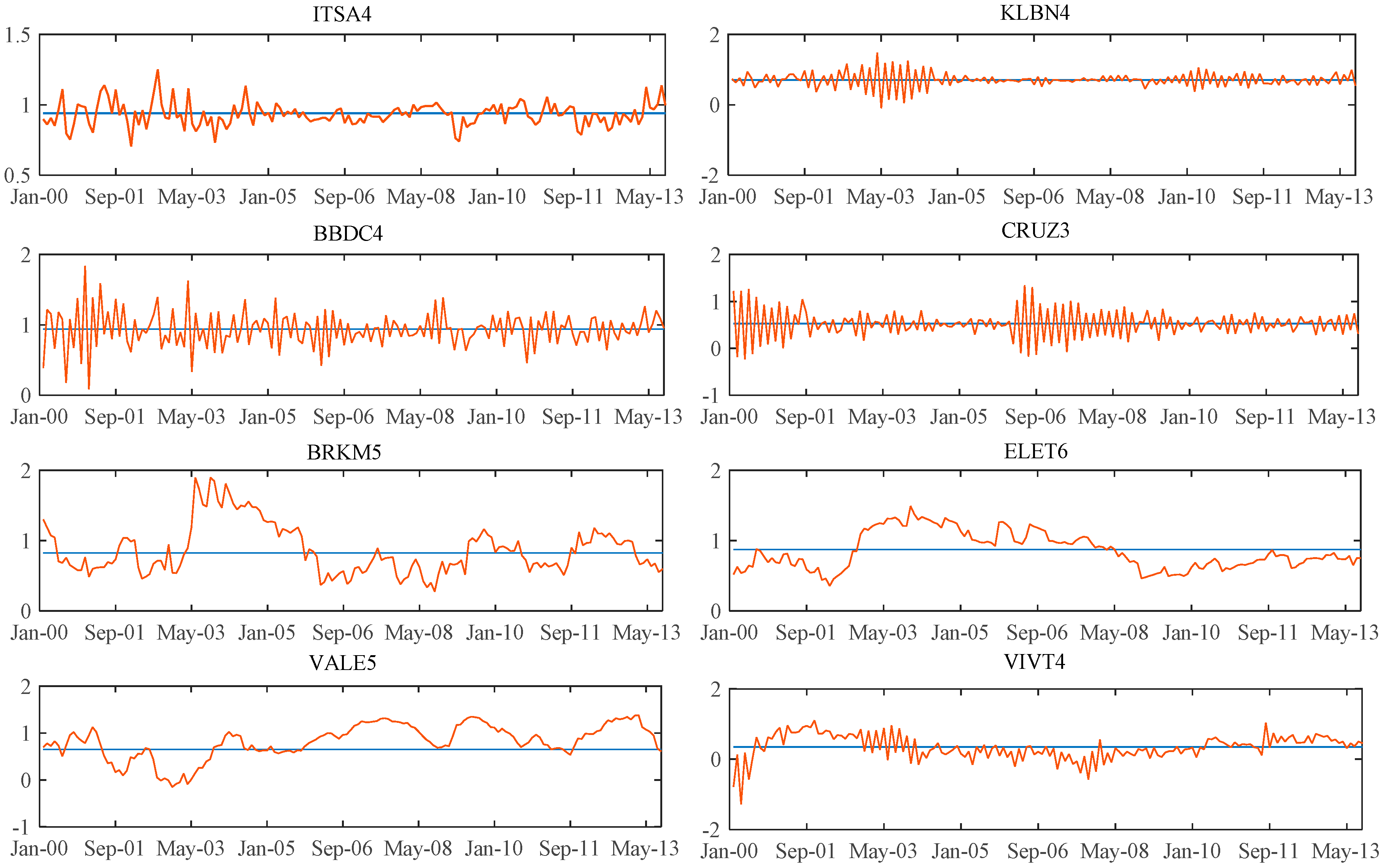
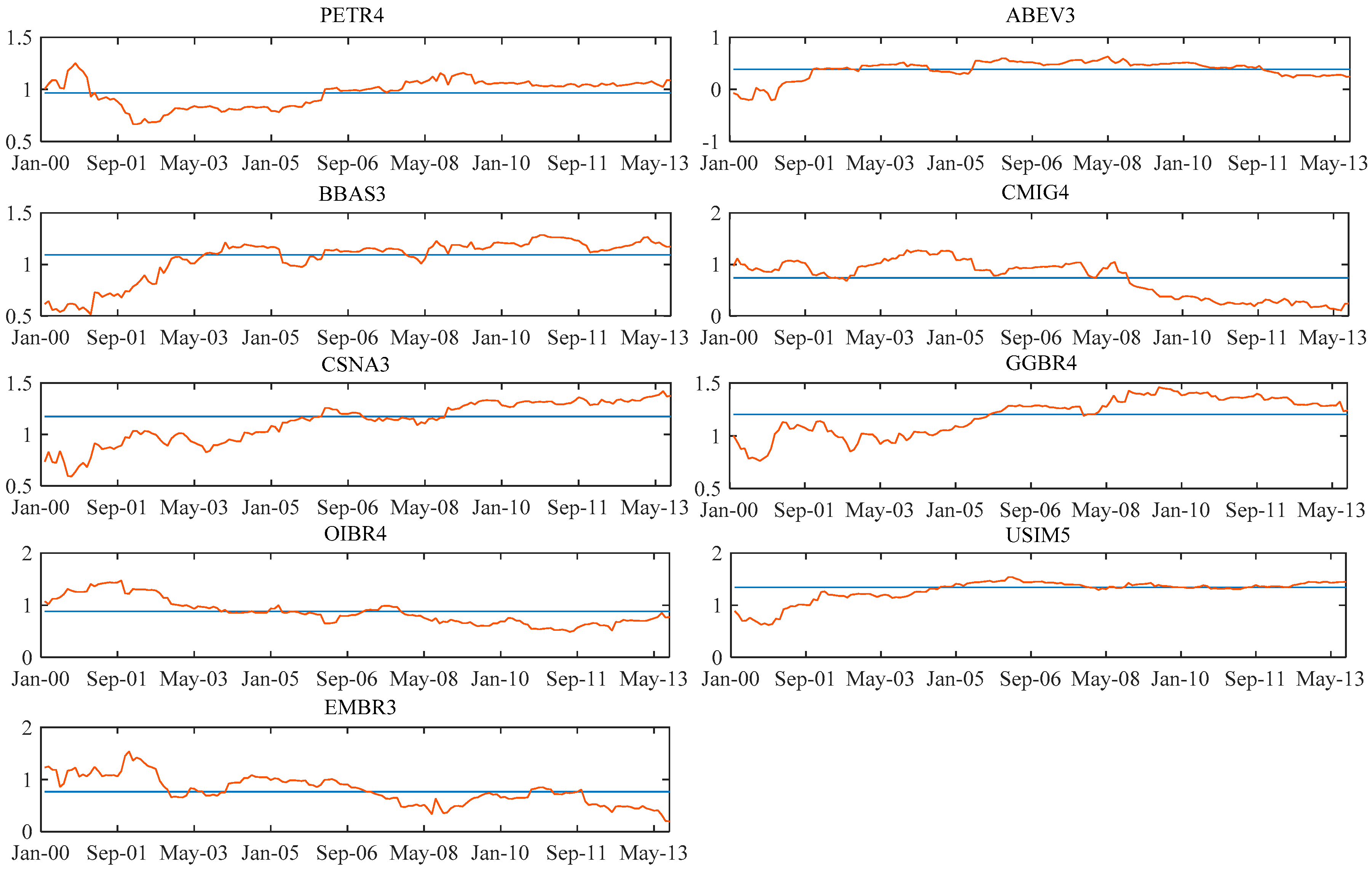
For the shares whose most significant models were the dynamic A&F, we represented in the graphs set C-1 of Appendix C the dynamic behavior of the beta versus its B (long-term beta) adapted by the Kalman filter. For the shares whose most significant models are the ones with beta following a random walk, we represent in the Appendix C, graphs set C-2, the dynamic behavior of the beta versus the fixed beta estimated by OLS in the traditional CAPM.

The C-2 graphs set provides evidence of the relationship between fixed betas of the CAPM obtained by OLS and dynamic betas obtained from the Kalman filter. An important point in the analysis of the results is the evidence of the proximity between the dynamic betas and the fixed betas. This occurs because of the assumption of the mean reversion that is intrinsic in the used filter, making the current estimated value of beta affected by the level of betas from the past.

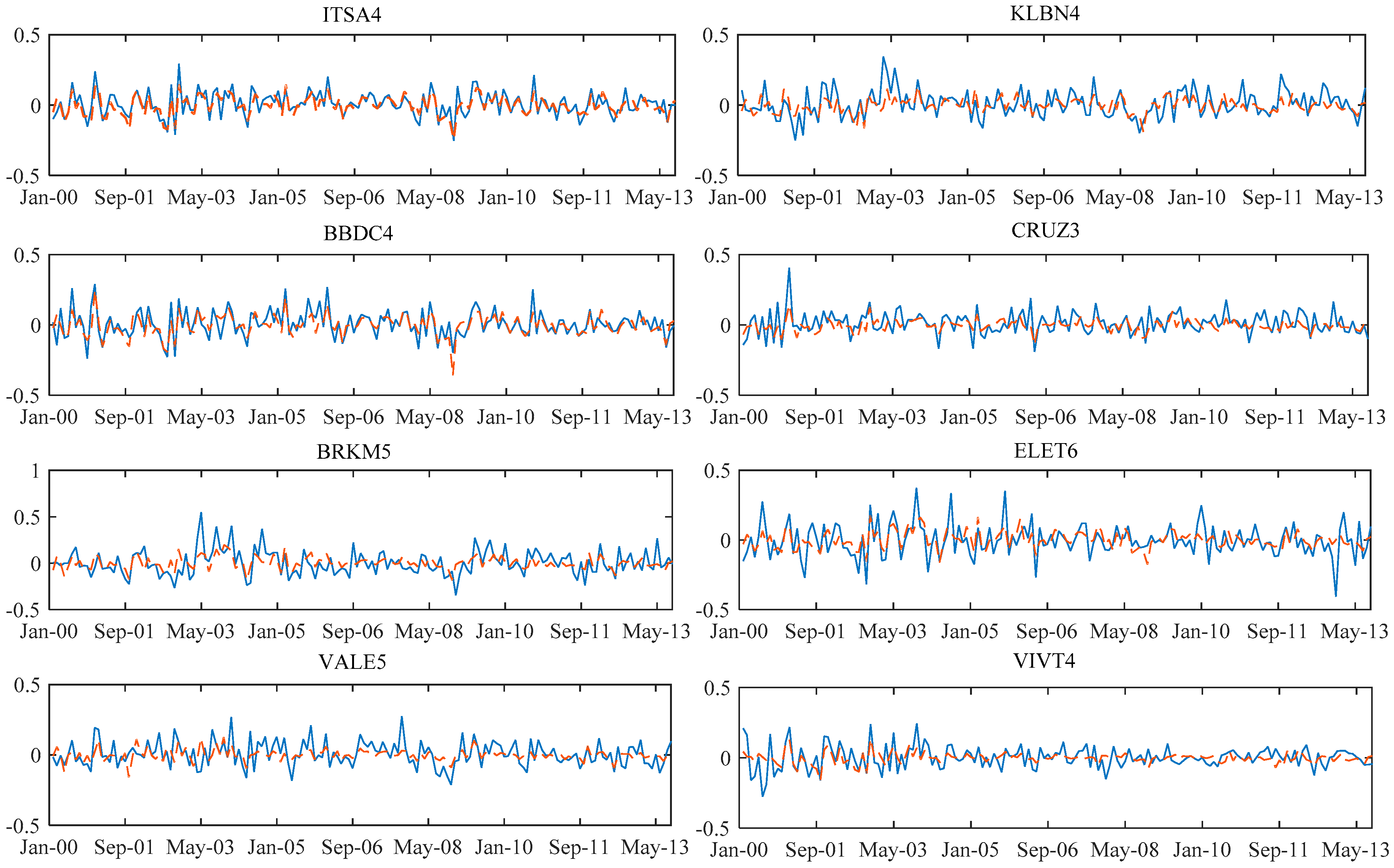
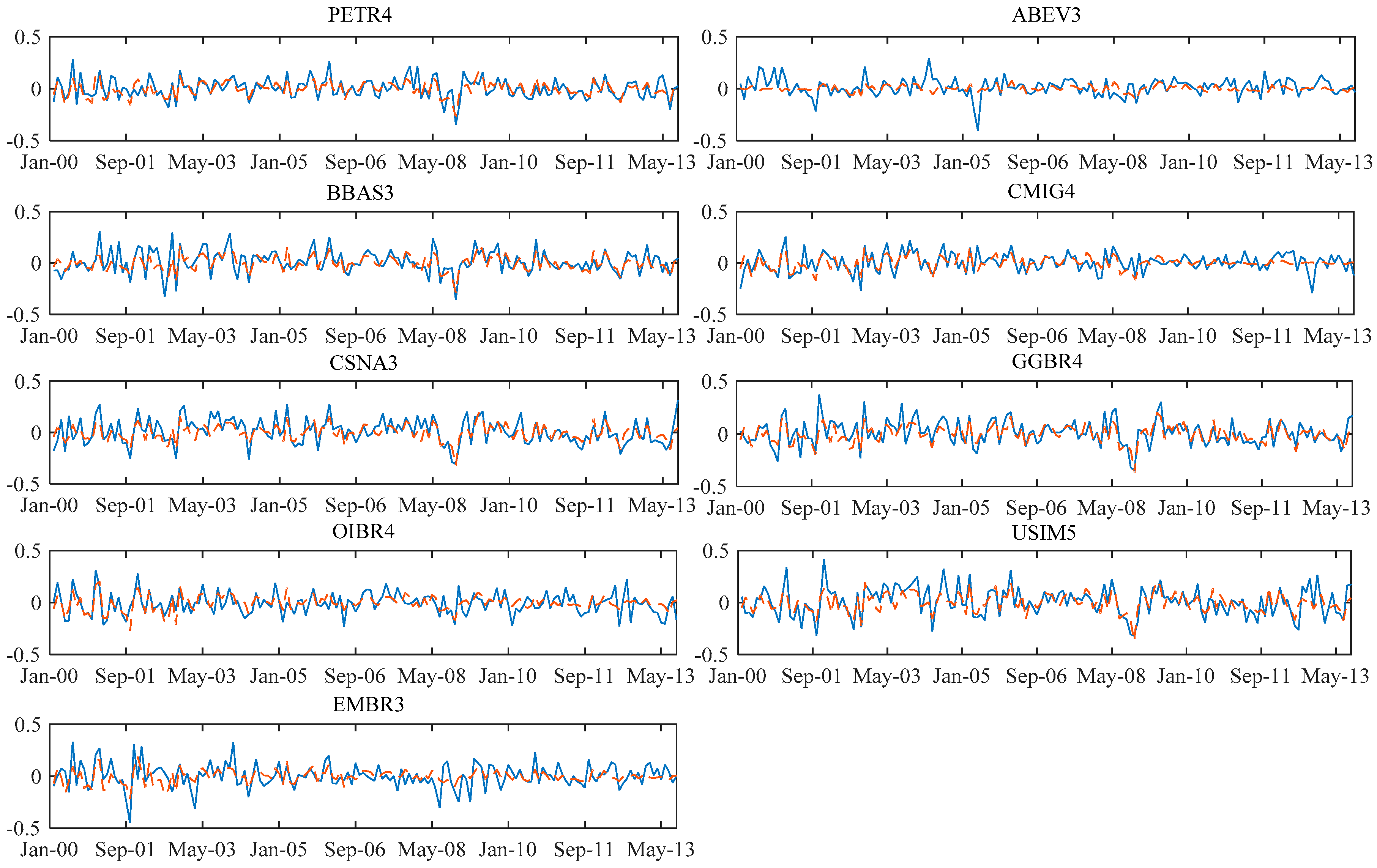
The graphs showing the result of the predicted return of the model of each share $R_{t+1|t}^i$ compared to the return that actually occurred in each time “t” are shown in Appendix D.

3.3. Learning CAPM Estimation Errors

To analyze the goodness-of-fit of the models, two measures of the asset pricing errors were calculated, the RMSE (Root Mean Squared Error) and CPE (Composite Pricing Error). The RMSE for each model and each share is reported in

Table 4. Result: root mean squared error.

RMSE (Root Mean Squared Error) Average
	No Variables	P/BV & P/E	SW Fixed	Energ. Consump.	All	Random Walk	OLS
PETR4	0.0662	0.0658	0.0659	0.0662	0.0650	0.0677	0.0660
ABEV3	0.0777	0.0769	0.0769	0.0770	0.0760	0.0794	0.0776
BBDC4	0.0672	0.0701	0.0658	0.0672	0.0672	0.0738	0.0704
BBAS3	0.0767	0.0751	0.0767	0.0768	0.0751	00778	0.0764
BRKM5	0.1168	0.1163	0.1167	0.1166	0.1161	0.1191	0.1189
ELET6	0.0986	0.0963	0.0986	0.1008	0.0943	0.0995	0.1005
CMIG4	0.0747	0.0715	0.0744	0.0743	0.0712	0.0744	0.0778
CSNA3	0.0870	0.0858	0.0867	0.0863	0.0849	0.0879	0.0855
GGBR4	0.0792	0.0785	0.0789	0.0789	0.0780	0.0802	0.0799
ITSA4	0.0566	0.0544	0.0562	0.0566	0.0541	0.0575	0.0565
KLBN4	0.0832	0.0832	0.0823	0.0831	0.0821	0.0847	0.0834
OIBR4	0.0851	0.0866	0.0844	0.0864	0.0862	0.0869	0.0864
CRUZ3	0.0712	0.0713	0.0721	0.0684	0.0681	0.0783	0.0750
USIM5	0.0949	0.0940	N.A.	0.0932	0.0929	0.0957	0.0948
VALE5	0.0759	0.0696	0.0715	0.0704	0.0666	0.0711	0.0736
VIVT4	0.0759	0.0705	0.0715	0.0759	0.0677	0.0764	0.0762
EMBR3	0.1062	0.1050	0.1060	0.1044	0.1031	0.1144	0.1072

Source: Elaborated by the Author.

below. We can observe that, systematically, the model with all conditioning variables has the lowest RMSE. This is in line with the findings of A&F.

In addition to the test above, we calculate the CPE that, due to its nature, gives lower weight to the alphas of the most volatile stocks. The result is reported in

Table 5. Result: composite pricing error.

CPE (Composite Pricing Error)
No Variables	P/BV & P/E	SW Fixed	Energ. Consump.	All	Random Walk	OLS
0.6851	0.5475	0.5782	0.6545	0.5310	0.5797	0.7334

Source: Elaborated by the Author.

.

Thus, on the whole result of RMSE and CPE parameters, the model with the best goodness-of-fit was using all the exogenous variables.

However, comparing the results of the model selection by the confidence level with the methodology of minor errors, RMSE and CPE, the conclusion is that they diverge. In the first, which uses the p-values for each estimated coefficient as indicators together with the information criteria for the selection of the best models, there was no selection of the one with all exogenous variables. However, in the methodology that uses RMSE and CPE, the model with all exogenous variables is preferred. This difference shows, therefore, that we must be careful when using the A&F methodology for simple shares, because the minor errors method could select models with low explanatory power of the betas behavior of each action.

4. VaR Calculation Using the Model Results

4.1. VaR Calculation

Using the results of the models above, we can calculate the VaR for each share studied in this work. Therefore, the starting point was the calculation of the historical parametric VaR with normal distribution, which is given by:

$$Va{R}_{ht,\phi }^i={\Psi }^{-1}(1-\phi ){\sigma }_{R^i}\sqrt{h}$$

where ${\Psi }^{-1}$ is the inverse cumulative function of the normal distribution; $\phi$ is the VaR significance level; ${\sigma }_{R^i}$ it is the standard deviation of asset “$i$” returns; $h$ is the VaR time horizon.

However, for this study, the calculation of VaR will differ from the traditional way, because the return of the asset $R^i$ in the case of the CAPM with random walk is given by:

$$R_t^i={\beta }_t^i{R}_t^M+{\mathsf{\eta }}_t^i$$

From this, it is not difficult to prove that the standard deviation of returns of asset “$i$” is equal to the idiosyncratic standard deviation of this asset, i.e., ${\sigma }_{R^i}={\sigma }_{{\mathsf{\eta }}^i}$. Thus, we have the VaR equation that can be rewritten as:

$$Va{R}_{ht,\phi }^i={\Psi }^{-1}(1-\phi ){\sigma }_{{\mathsf{\eta }}^i}\sqrt{h}$$

(18)

Therefore, to calculate the VaR of each asset, we used the idiosyncratic deviations from the return of shares ${\sigma }_{{\mathsf{\eta }}^i}$, whose learning dynamic models were estimated previously.

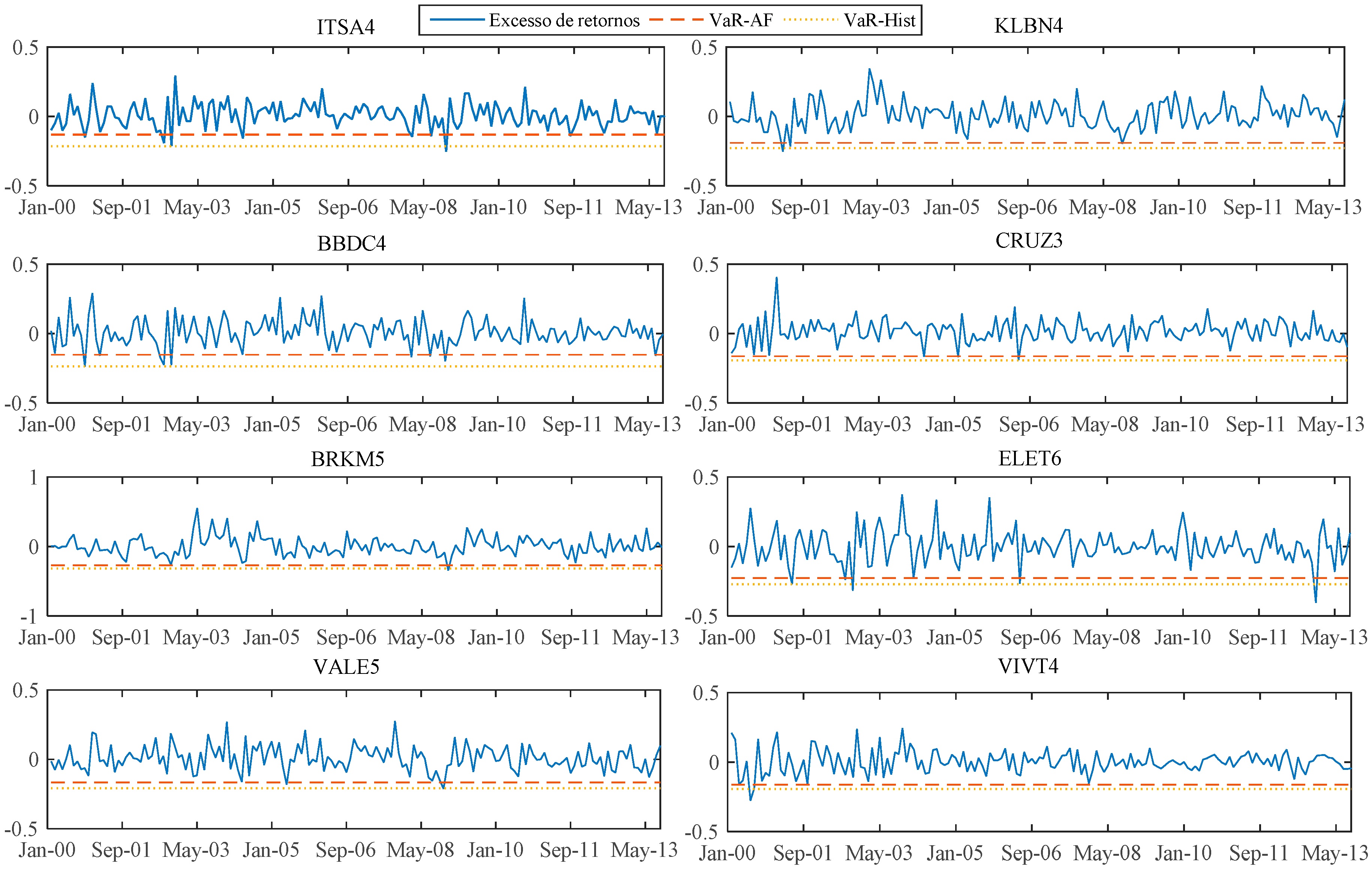
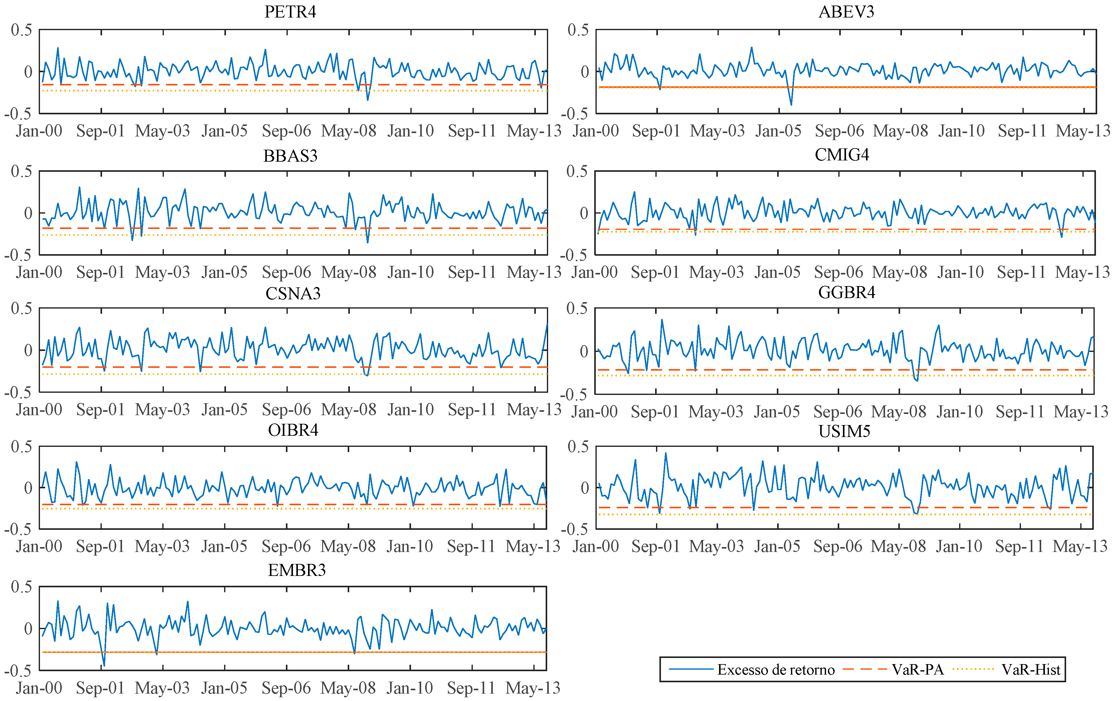
The results of the VaR calculation using the dynamic beta methodology were compared with the historical parametric VaR methodology results in order to test its relative efficiency to the traditional method. For that, we calculated the VaR using the two methods with a one-month time horizon for the significance levels of 1% and 5%. The results are shown in Appendix E.

4.2. Backtesting Results

In order to test the efficiency of the proposed model to calculate the VaR, there were applied two widely recognized backtesting methodologies to the results, which are the Unconditional Convergence Kupiec (1995) Test and the Christoffersen (1998) Independence Test. The first one measures, through a ${\chi }^2$ statistics created by Kupiec, the unconditional percentage of violations of the VaR in a given period. The second measures, through another ${\chi }^2$ statistics created by Christoffersen, the percentage of violations of the VaR and the persistence of this violation, showing the dependency on the previous violation. The combined statistic of these two methods brings the final backtesting result of the VaR. In both tests of Kupiec and Christoffersen, including the combined result, we used 95% and 99% confidence levels, which are the recommended levels in the RiskMetrics (1996) manual.

The backtesting results calculated for the group of 17 stocks are in

Table 6. Backtesting.

Test	CAPM Models
	No Variables		P/VPA & P/L		SWAP360		Energy Consump.
	VaR 95%	VaR 99%	VaR 95%	VaR 99%	VaR 95%	VaR 99%	VaR 95%	VaR 99%
Unconditional Convergence Test (Kupiec)	76%	53%	71%	53%	76%	59%	76%	65%
Independence Test (Christoffersen)	59%	47%	59%	47%	65%	53%	65%	53%
Conditional Convergence Test (combined)	59%	53%	65%	53%	59%	59%	65%	59%

and

Table 7. Backtesting (CONT.)

Test	CAPM Models
	All		Random W.		OLS		Historical VaR
	VaR 95%	VaR 99%	VaR 95%	VaR 99%	VaR 95%	VaR 99%	VaR 95%	VaR 99%
Unconditional Convergence Test (Kupiec)	71%	47%	82%	71%	100%	100%	100%	100%
Independence Test (Christoffersen)	59%	47%	71%	59%	82%	88%	82%	88%
Conditional Convergence Test (combined)	59%	47%	71%	65%	82%	100%	82%	100%

Source: Elaborated by the Author.

below. The values represent the percentage of models in this group of shares that succeeded in the tests for each backtesting methodology in a one-month time horizon and confidence levels of 95% and 99%.

As shown, none of dynamic models, including CAPM model with random walk, succeeded in 100% of the tests for confidence levels of 95% and 99%. However, VaR models with the OLS model and the historical VaR succeeded in 100% of the shares for the confidence level of 99%.

These results demonstrate a very relevant fact on the use of VaR calculation methodology with idiosyncratic deviation of returns on the assets. Using this methodology, as shown in the E-1 graphs, Appendix E, the VaR adjustment of the model on past returns is greater than the adjustment of the historical VaR, i.e., the distance between returns and the VaR waterline of the dynamic model is smaller. Thus, in some models whose backtestings were not favorable, the VaR waterlines were too close to the real returns, increasing the likelihood of violations. However, there was a percentage above 50% of VaR acceptance on all models, i.e., in more than half of the shares dynamic models could be used to calculate VaR.

Therefore, we can conclude that the use of VaR methodology with dynamic models is less conservative than the traditional calculation of historical VaR. However, although less conservative, the dynamic models’ methodology succeeded in several of the performed tests, showing that, depending on the share and the confidence level to be used, the method can be applied. Therefore, investors who want to use a less conservative approach, but that is efficient in the VaR calculation depending on the analyzed asset, can use the proposed dynamic models without losses above the confidence level.

5. Final Remarks

This study has adapted the conditional CAPM with learning processes proposed by Adrian and Franzoni (2009) to the Brazilian financial market. Specifically, there were used the shares from the BOVESPA stock exchange that presented quote data and book value from September 1999 to September 2013 and were part of the Bovespa Index. A dynamic model for the evolution of the CAPM betas was estimated. In the equation, we included various conditioning variables included in other studies of the Brazilian literature (Flister et al. (2011), Mazzeu et al. (2013) and Fischberg Blank et al. (2014)). Due to limitation of databases, some modifications had to be made for performing this work. We used monthly data rather than quarterly data; the analyses were made using the shares rather than stock portfolios and we used a few different exogenous conditioning variables.

As in the A&F results, many of the estimated models did not exhibit acceptable levels of confidence. Thus, in this study, it was included and estimated new dynamic CAPM models with the beta behaving like random walk, obtaining results that are more satisfactory.

In the selection of models with better fit, two criteria were used: the first was the Root Mean Squared Error (RMSE) jointly to the Composite Pricing Error (CPE). Table 5 and Table 6 show the results in terms of goodness-of-fit. In the second, we introduce other criteria, namely, the significance of the model parameters jointly with information criteria. Thus, we came up to models with greater significance in explaining the betas behavior. The minimum confidence level used to select was 90% for each coefficient. Table 3 and Table 4 show the best models in terms of significance. The results were different from those found in the selection of models from the average prediction errors, bringing a new perspective to the use of such models.

As explained in this work, the simple use of the learning CAPM model to estimate the dynamic beta for shares in Brazil already demonstrated a gain in quality compared to the traditional OLS model with fixed CAPM betas. Therefore, given that the model takes into account dynamic betas varying according to an autoregressive process of order one, we conclude that the sensitivity of the return of a share depends on its value in the previous period.

For some Brazilian stocks, in addition to this autoregressive behavior of betas, other factors influence the variation of them. As an example, the model that best explains the betas behavior of the only two private banks’ shares (BBDC4 and ITSA4) has as exogenous variable the “SWAP 360”, which is the country’s interest spread. Other stocks whose models were chosen using the SWAP 360 were KLBN4 and VALE5.

The models’ selection method that choose the model according to the confidence levels of the shares also indicated for BRKM5 and ELET6 shares the A&F dynamic models without exogenous variables, indicating that the behavior of their betas follows a long-term trend.

In addition, the CRUZ3 share was the only one that got the A&F model with exogenous variable being consumption rate (that as a proxy considered the electricity consumption) as the selected model.

On the other hand, the VIVT4 share was the only one that got the A&F model with variables related to the share price as the selected model.

In the other nine remaining shares, the models with the best confidence percentages were the dynamic with beta behaving as random walk.

As can be seen, the results were different, depending on the analyzed share. This is one of the main contributions of this work, the conclusion that shares alone follow different dynamic models in the evolution of their betas. This contrasts with the empirical findings for stock portfolio returns.

The results obtained taking into account the significance criteria differ from those using only the minimum error criteria, RMSE and CPE, used by A&F. Therefore, if we use the model with minor errors, we end up selecting models with low explanatory power.

An additional analysis in the present study was the use of dynamic CAPM model with learning in the calculation of VaR—Value-at-Risk, following the Sommacampagna (2002) proposal. However, unlike the author, the dynamic CAPM models including exogenous variables were used, bringing new results. The VaR calculations were made for confidence levels of 95% and 99% with the time horizon of one month.

To test the assertiveness of the new VaR calculation method, the backtesting methodologies of Kupiec (1995), Christoffersen (1998) and a combination of both, were applied to the results. The final result showed that none of the dynamic models, including CAPM model with random walk, succeeded in 100% of the tests for confidence levels of 95% and 99%. However, VaR models with the OLS model and the historical VaR succeeded in 100% of the shares to the confidence level of 99%.

We conclude from this study that the VAR goodness-of-fit of the dynamic models related to the past returns is better than the goodness-of-fit of the historical VaR, i.e., the distance between past returns and the VaR waterline of the dynamic model is lower. Thus, in models whose backtesting were not favorable, the VaR waterline was too close to the past returns, increasing the probability of failure.

Thus, it can be concluded that the use of the VaR methodology with dynamic models is less conservative than the traditional calculation using the historical VaR.

References

1. Adrian, Tobias, and Francesco Franzoni. 2009. Learning about beta: Time-varying factor loadings, expected returns, and the conditional CAPM. Journal of Empirical Finance 16: 537–56. [Google Scholar] [CrossRef]
2. Almeida, Leandro de Oliveira. 2010. Estimação do CAPM Intertemporal com Ações da Bovespa. Paulo: Universidade de São Paulo. [Google Scholar]
3. Breeden, Douglas T. 1979. An Intertemporal Asset Pricing Model with Stochastic Consumption and Investment Opportunities. Journal of Financial Economics 7: 265–96. [Google Scholar] [CrossRef]
4. Campbell, John Y., and Tuomo Vuolteenaho. 2004. Bad beta, good beta. American Economic Review 94: 1249–75. [Google Scholar] [CrossRef] [Green Version]
5. Christoffersen, Peter F. 1998. Evaluating Interval Forecasts. International Economic Review 39: 841–62. [Google Scholar] [CrossRef]
6. Fama, Eugene F., and Kenneth R. French. 1993. Common risk factors in the returns on stocks and bonds. Journal of Financial Economics 33: 3–56. [Google Scholar] [CrossRef]
7. Ferson, Wayne E., and Campbell R. Harvey. 1999. Conditioning Variables and the Cross Section of Stock Returns. The Journal of Finance 54: 1325–60. [Google Scholar] [CrossRef]
8. Fischberg Blank, Frances, Carlos Patricio Samanez, Tara Keshar Nanda Baidya, and Fernando Antonio Lucena Aiube. 2014. CAPM Condicional: Betas Variantes no Tempo no Mercado Brasileiro. Revista Brasileira de Finanças 12: 163–99. [Google Scholar]
9. Flister, Valle E., Frederico, Aureliano Angel Bressan, and Hudson Fernandes Amaral. 2011. CAPM Condicional no Mercado Brasileiro: Um Estudo dos Efeitos Momento, Tamanho e Book-to-Market entre 1995 e 2008. Revista Brasileira de Finanças 9: 105–29. [Google Scholar]
10. Jagannathan, Ravi, and Zhenyu Wang. 1996. The conditional CAPM and the cross-section of expected returns. Journal of Finance 51: 3–53. [Google Scholar] [CrossRef]
11. Koutmos, Dimitrios. 2012. Time-Varying Behavior of Stock Prices, Volatility Dynamics and Beta Risk in Industry Sector Indices of the Shanghai Stock Exchange. Accounting and Finance Research 1: 109–25. [Google Scholar] [CrossRef]
12. Kupiec, Paul H. 1995. Techniques for Verifying the Accuracy of Risk Management Models. Journal of Derivatives 3: 73–84. [Google Scholar] [CrossRef]
13. Lettau, Martin, and Sydney Ludvigson. 2001. Resurrecting the (C)CAPM: A cross-sectional test when risk premia are time-varying. Journal of Political Economy 109: 1238–87. [Google Scholar] [CrossRef]
14. Lewellen, Jonathan, and Stefan Nagel. 2006. The conditional CAPM does not explain asset-pricing anomalies. Journal of Financial Economics 82: 289–314. [Google Scholar] [CrossRef]
15. Lintner, John. 1965. The valuation of risk assets and selection of risky investments in stocks portfolios and capital budgets. Review of Economics and Statistics 47: 13–37. [Google Scholar] [CrossRef]
16. Machado, Octavio Portolano, Adriana Bruscato Bortoluzzo, Śergio Ricardo Martins, and Antonio Zoratto Sanvicente. 2013. Inter-temporal CAPM: An Empirical Test with Brazilian Market Data. Revista Brasileira de Finanças 11: 149–80. [Google Scholar]
17. Markowitz, Harry M. 1959. Portfolio Selection: Efficient Diversification of Investments. New York: John Wiley & Sons. [Google Scholar]
18. Mazzeu, João Henrique Gonçalves, and André Alves Portela Santos. 2013. CAPM condicional com aprendizagem aplicado ao mercado brasileiro de ações. Revista de Administração Mackenzie 14: 143–75. [Google Scholar] [CrossRef]
19. Merton, Robert C. 1973. An Analytic Deviation of the Efficient Portfolio Frontier. The Journal of Financial and Quantitative Analysis 7: 1851–72. [Google Scholar] [CrossRef]
20. Mossin, Jan. 1966. Equilibrium in a capital asset market. Econometrica 34: 768–83. [Google Scholar] [CrossRef]
21. RiskMetrics. 1996. Technical Document, 4th ed. New York: J.P.Morgan/Reuters. [Google Scholar]
22. Rockinger, Michael, and Giovanni Urga. 2001. A Time Varying Parameter Model to Test for Predictability and Integration in the Stock Markets of Transition Economies. Journal of Business & Economic Statistics 19: 73–84. [Google Scholar]
23. Ross, Stephen A. 1976a. The arbitrage theory of capital asset pricing. Journal of Economic Theory 13: 341–60. [Google Scholar] [CrossRef]
24. Ross, Stephen A. 1976b. Risk, return, and arbitrage. Risk and Return in Finance 1: 189–218. [Google Scholar]
25. Sharpe, William F. 1964. Capital asset prices: A theory of market equilibrium under conditions at risk. Journal of Finance 19: 425–42. [Google Scholar]
26. Sommacampagna, Cristina. 2002. Estimating Value at Risk with the Kalman Filter, Dipartimento Studi Finanziari. Verona: Università di Verona. [Google Scholar]
27. Treynor, Jack L. 1961. Market Value, Time, and Risk. Available online: https://ssrn.com/abstract=2600356 or http://dx.doi.org/10.2139/ssrn.2600356 (accessed on 10 July 2016).
28. Treynor, Jack L. 1962. Toward Theory of Market Value of Risky Assets. London: Risk Books. [Google Scholar]
1
The reference exchange rate for the US dollar, known in the market as the PTAX rate, which is the arithmetic average of four daily requests from foreign exchange dealers for bid/offer rates.