Impact of Cost Efficiency on Bank Capital and the Cost of Financial Intermediation: Evidence from BRICS Countries

Abstract

Over last two decades, emerging and developing nations have desperately endeavored for efficient banking sectors. In this study, we argue that bank efficiency generates incentives that can impact banks’ capital holdings and the cost of financial intermediation. Analyzing a panel dataset of 1190 banks from BRICS (Brazil, Russia, India, China, South Africa) countries over the period 2007–2015, we find robust evidence that more efficient banks hold higher capital and charge lower financial intermediation costs. In an extended sample over the period 2000–2015, we observe that cost efficiency had a marginal positive impact on bank capital during the global financial crisis of 2007–2009. We also observe that on average, banks increased the cost of financial intermediation during the crisis, however, greater efficiency helped banks to not charge higher intermediation costs. Our results imply the beneficial impact of bank efficiency for bank stability and real economy.

1. Introduction

In response to the global financial crisis (GFC) of 2007–2009, regulatory authorities in many countries have adopted stringent capital requirements in the form of Basel-III for banks to ensure future financial stability. Despite this stated objective of financial stability, some scholars criticize stringent capital requirements for their negative effects. For instance, one strand of the extant literature argues that holding higher capital is ‘too expensive’ and would jeopardize the banks’ ability to lend, increase the bank lending rates, and, consequently, would adversely affect the economic output (IIF 2011; Wong et al. 2010; Slovik and Cournède 2011).

On the other hand, a parallel strand of the literature argues that there are multiple factors which impact the banks’ choice of holding capital, and stringent capital requirements are likely to have no or little impact. For example, Gropp and Heider (2010) find that banks adjust their equity ratios according to their target capital structure, and capital regulation has only a second order importance for them. Similarly, Admati and Hellwig (2013) argue that equity is ‘not expensive’ and suggest even higher equity ratios (i.e., 20 to 30 percent). They argue that equity appears expensive because debt is subsidized by tax-payer-backed deposit insurance and bailout schemes, and suggest that maintaining higher equity ratios wouldn’t increase credit cost. Fonseca and González (2010) find that bank market power and capital levels have a positive association. Contributing to this latter literature, we examine whether bank cost efficiency impacts bank capital. We also examine the impact of cost efficiency on banks’ cost of financial intermediation.

Cost efficiency is an important bank-level factor that can impact bank capital and the cost of financial intermediation (Agapova and McNulty 2016; Berger and Bonaccorsi di Patti 2006). Berger and Bonaccorsi di Patti (2006) suggested two competing hypotheses to explain the impact of bank efficiency on capital: franchise-value and efficiency-risk hypotheses. The franchise-value hypothesis argues that more efficient banks tend to choose relatively high equity ratios to protect the future income derived from high firm efficiency and predict a positive impact of efficiency on bank capital. On the contrary, the efficiency-risk hypothesis argues that more efficient banks may hold relatively low equity ratios, as higher expected returns from the greater bank efficiency substitutes to some degree for equity capital in protecting the firm against bankruptcy or liquidation.

Similarly, we argue that more efficient banks can charge a higher cost of financial intermediation by minimizing the prices on inputs, such as deposits and borrowed funds, and maximizing the prices on outputs, such as loans. On the contrary, they may also charge a lower cost of financial intermediation to pass on the savings due to cost efficiency to depositors and borrowers to increase market share.

For empirical analysis, we use a panel dataset of 1190 BRICS (Brazil, Russia, India, China, South Africa) banks over the period from 2007 to 2015. There are at least two reasons to focus on BRICS banks. First, some scholars such as Jacobs and Van Rossem (2014) argue that the robust economic growth over last few decades and the minimal effect of the global financial crisis on the BRICS block has turned the world’s attention to these countries. In such a scenario, the better understanding of BRICS countries’ banking sectors is even more important. Second, BRICS is a group of five emerging economies where financial sector reforms are still a work in progress. These reforms are causing variations in bank efficiency in these countries and offer an ideal laboratory to examine our postulates. For example, Wanke et al. (2015) observe that the Brazilian government’s aggressive reduction in the SELIC (Sistema Especial de Liquidação e Custodia) (i.e., the base-interest rate of Brazilian economy) and subsidized credit policies for real estate financing in 2007 have substantially impacted the efficiency of Brazilian banks. Ataullah and Le (2006) found that economic reforms, such as fiscal reforms, financial reforms, and private investment liberalization have significantly affected the efficiency of Indian banks. Huang et al. (2017) find that all types of Chinese banks have upward trend in efficiency scores in fund collection and revenue generation activities over the period of 2004–2013 due to Chinese financial reforms. The Chinese government has initiated reforms such as opening up the banking sector to outside world, diversification of ownership of Chinese banks, and minimizing the government’s capital subsidies, among others. Financial sector reforms are also underway in other BRICS block members (Wanke et al. 2017).

We employ a two-step system generalized method of moments (GMM) estimator to account for the endogeneity problem due to reverse causality from capital requirements to bank cost efficiency. Since the cost efficiency measures how efficient banks are relative to best-practice in transforming their inputs (e.g., deposits) to outputs (e.g., loans), therefore, capital requirements may affect bank efficiency by influencing the mix of financing sources in bank capital structure and the allocation of bank assets portfolios. In this context, a number of recent studies have examined the impact of capital regulation on bank efficiency (Alam 2012; Carvallo and Kasman 2017; Manlagnit 2015; Pasiouras 2008; Pasiouras et al. 2009). All these studies have examined the effect of equity ratios on bank efficiency. In this study, we model the relation the other way around to examine the impact of bank cost efficiency on equity ratios while controlling for the reverse causality.

Previewing the main results, we find robust evidence that cost efficiency has a positive impact on bank equity ratios and a negative effect on the cost of financial intermediation. These results hold to several robustness tests.

This study contributes to existing literature in several ways. First, we contribute to the literature which examines the impact of bank efficiency on capital. To best of our knowledge, to date, only Berger and Bonaccorsi di Patti (2006) have focused on this relation for the US banks. We explicitly examine this relation for BRICS block. In this regard, we complement the recent studies which examine the impact of financial regulations, especially the capital requirements, on bank efficiency (Alam 2012; Carvallo and Kasman 2017; Manlagnit 2015; Pasiouras 2008; Pasiouras et al. 2009). We examine this relation the other way around from bank efficiency to capital ratios. Second, we examine the impact of bank cost efficiency on banks’ cost of financial intermediation. To the best of our knowledge, this study is the first one to specifically consider this channel.

The rest of the paper proceeds as follows: Section 2 presents the hypotheses; Section 3 introduces the sample and variables; Section 4 presents the empirical methodology; Section 5 reports empirical results; and the final section concludes the study and draws practical implications.

2. Hypotheses Development

In this paper, we aim to examine the impact of bank cost efficiency on bank capital and cost of financial intermediation. In this section, we establish the testable hypotheses that how bank efficiency impacts bank capital and the cost of financial intermedation.

Berger and Bonaccorsi di Patti (2006) suggest two competing hypotheses to explain the impact of bank efficiency on capital: franchise-value and efficiency-risk hypotheses. The efficiency-risk hypothesis predicts a positive impact of bank efficiency on bank capital. According to the efficiency-risk hypothesis, efficient banks are likely to choose lower capital ratios than other banks, because if all else are equal, the higher bank efficiency reduces the expected financial distress and bankruptcy costs for the banks. For a given capital structure, higher bank efficiency generates higher expected returns that can substitute to some degree for the equity capital in protecting the bank against future financial crises. Under this hypothesis, bank efficiency first positively impacts the expected returns and then the higher expected returns from bank efficiency substitute for equity capital to manage bank risk. On the other hand, the franchise-value hypothesis predicts a negative impact of bank efficiency on bank capital. According to this hypothesis, efficient banks are likely to generate more expected income for bank owners. This higher expected income acts as an economic rent or franchise value and encourages banks to choose higher equity ratios to protect these rents from financial distress or liquidation. In their empirical anlysis, Berger and Bonaccorsi di Patti (2006) could not find the strict dominance of one hypothesis over the other. Based on these hypotheses, we are priori uncertain about the impact of bank efficiency on bank capital.

To the best of our knowledge, no prior literature is available that explicitly discusses the impact of bank efficiency on banks’ cost of financial intermediation. We argue that both positive and negative association is expected between bank efficiency and the cost of financial intermediation. For the former, more efficient banks can negotiate optimal contracts with both lenders (e.g., depositors and debt-holders) and borrowers. Through optimal contracting, efficient banks would be able to minimize prices on inputs, such as deposits and borrowed funds, and maximize prices on outputs, such as loans. Lower rates paid to depositors alongside higher rates charged to borrowers would widen the banks’ cost of financial intermediation. For the latter, more efficient banks are better positioned to pass on the savings due to cost efficiency to depositors and borrowers. They may pay higher interest rates to depositors and charge lower rates on loans to increase market share as compared less efficient banks. Higher interest rates paid on deposits and lower rates charged on loans would narrow the banks’ cost of financial intermediation. Based on these arguments, we expect that the impact of bank efficiency on banks’ cost of financial intermediation is uncertain and may be positive or negative.

3. Sample and Variables

3.1. Study Sample

For sample construction, we downloaded the balance sheet and income statement accounting data of commercial, savings, cooperative, investment, and foreign banks of 5 BRICS emerging economies from Bankscope database over the period 2007–2015. Then we collected data for macroeconomic variables from World Development Indicators (WDI)1 database of the World Bank for BRICS countries over the same period. Finally, we linked bank-level annual data with country-level annual data of macroeconomic variables. From this dataset, we deleted observations with missing values for key bank- or country-level variables. We also deleted banks with less than two observations over the sample period. After applying all filters, our final dataset is an unbalanced panel with 7887 annual observations for 1190 banks over the period 2007–2015. The number of banks varies from country to country, with 793 banks for Russia, 154 for China, 123 for Brazil, 90 for India, and 30 for South Africa.

3.2. Variables Definitions

Table 1. Description of the Variables.

Variables		Symbol	Description	Data/Variable Sources
Dependent Variables
Bank capital		OETTA	Equals the ratio of shareholders equity to total assets.	Bankscope
		REG_CAP	Equals the ratio of regulatory capital to total assets	Bankscope
Banks’ cost of intermediation		NIM1	Equals the ratio of net interest income over average total earning assets	Authors’ calculations based on Bankscope
		NIM2	Equals the ratio of net interest income over average total assets	Authors’ calculations based on Bankscope
Principal Variable
Cost efficiency		COSTEFF	Used stochastic frontier 4.1 version	Authors’ calculations based on Bankscope
	Total cost	TC	Natural logarithm of the summation of total interest expenses and operating expenses	Bankscope
	Inputs
	Price of labor	PL	Logarithm of personal expenses over total assets	Bankscope
	Price of fixed assets	PF	Logarithm of depreciation cost over fixed assets	Bankscope
	Price of fund	PF	Logarithm of total interest expenses on deposit over total deposit	Bankscope
	Outputs
	Total loans	TL	Logarithm of total loans	Bankscope
	Other earning assets	OEA	Logarithm of other earning assets	Bankscope
Bank Independent Control Variables
Implicit cost		IMPLICOST	Non-interest expenses relative to non-interest incomes	Authors’ calculations based on Bankscope
Management efficiency		MANEFF	The ratio of earning assets to total assets.	Authors’ calculations based on Bankscope
Bank size		SIZE	Natural logarithm of total assets	Authors’ calculations based on Bankscope
Deposit insurance dummy		DEPOD	A dummy variable that takes a value of one if the country has deposit insurance, and zero otherwise.	(Demirgüç-Kunt et al. 2005)
Ownership dummy		OWND	Equals 1 for the banks are owned by private shareholders and 0 for the banks owned by state government	(Zheng et al. 2017b)
Firm performance		PER	Equals the ratio of pre-tax profit over total assets	(Zheng et al. 2017a)
Leverage		LEV	Equals total debt over total assets of each bank	(Rahman et al. 2017)
Industry-specific
Hirschman–Herfindahl index		HHI	Sum of square of market share is a proxy for market concentration variable	Authors’ calculations
Macroeconomic Variables
Inflation, consumer prices (annual %)		INF	Annual rate of inflation (%)	World Development Indicators (WDI)
GDP growth (annual %)		GDP	Annual growth of GDP	World Development Indicators (WDI)
Financial crisis variable
Crisis dummy		CRISISD	A dummy variable that equals 1 for the years 2007 to 2009, and zero otherwise.	Authors’ idea

summarizes the variables employed in this study.

Bank capital and cost of financial intermediation are two main dependent variables. Following Ashraf et al. (2016c), we measure bank capital with two alternative proxies: OETTA and REG_CAP. OETTA equals the ratio of bank shareholders’ equity over total assets. REG_CAP equals the regulatory capital to total risk-weighted assets.

Banks’ cost of financial intermediation is also measured with two alternative proxies: NIM1 and NIM2. NIM1 equals the ratio of net interest revenue over average interest-bearing assets (Ashraf 2017a). NIM2 equals the ratio of net interest income over average total assets.

COSTEFF is main independent variable and is represented with annual cost efficiency scores for each bank. We use the Stochastic Frontier Analysis (SFA) approach to generate annual cost efficiency scores. This approach has been widely used to measure a firms’ efficiency (Kumbhakar and Lovell 2003). We estimated the following equation for cost efficiency scores.

$$\begin{array}{cc}\hfill {\mathrm{lnTC}}_{\mathrm{it}}=\mathrm{C}+{\displaystyle {\displaystyle \sum }_{\mathrm{n}=1}^3}& {\mathsf{\beta }}_{\mathrm{n}}{\ln \mathrm{P}}_{\mathrm{nit}}+{\displaystyle {\displaystyle \sum }_{\mathrm{k}=1}^2}{\mathsf{\delta }}_{\mathrm{k}}{\mathrm{lnY}}_{\mathrm{kit}}+{\displaystyle {\displaystyle \sum }_{\mathrm{n}=1}^3}{\displaystyle {\displaystyle \sum }_{\mathrm{m}=1}^3}{\mathsf{\beta }}_{\mathrm{nm}}\ln {\mathrm{P}}_{\mathrm{nit}}{\mathrm{lnP}}_{\mathrm{mit}}\hfill \\ & +{\displaystyle {\displaystyle \sum }_{\mathrm{k}=1}^2}{\displaystyle {\displaystyle \sum }_{\mathrm{j}=1}^2}{\mathsf{\delta }}_{\mathrm{kj}}\ln {\mathrm{Y}}_{\mathrm{kit}}{\mathrm{lnY}}_{\mathrm{jit}}+{\displaystyle {\displaystyle \sum }_{\mathrm{n}=1}^3}{\displaystyle {\displaystyle \sum }_{\mathrm{k}=1}^2}{\mathsf{\gamma }}_{\mathrm{nk}}\ln {\mathrm{P}}_{\mathrm{nit}}{\mathrm{lnY}}_{\mathrm{kit}}+{\in }_{\mathrm{it}}\hfill \end{array}$$

(1)

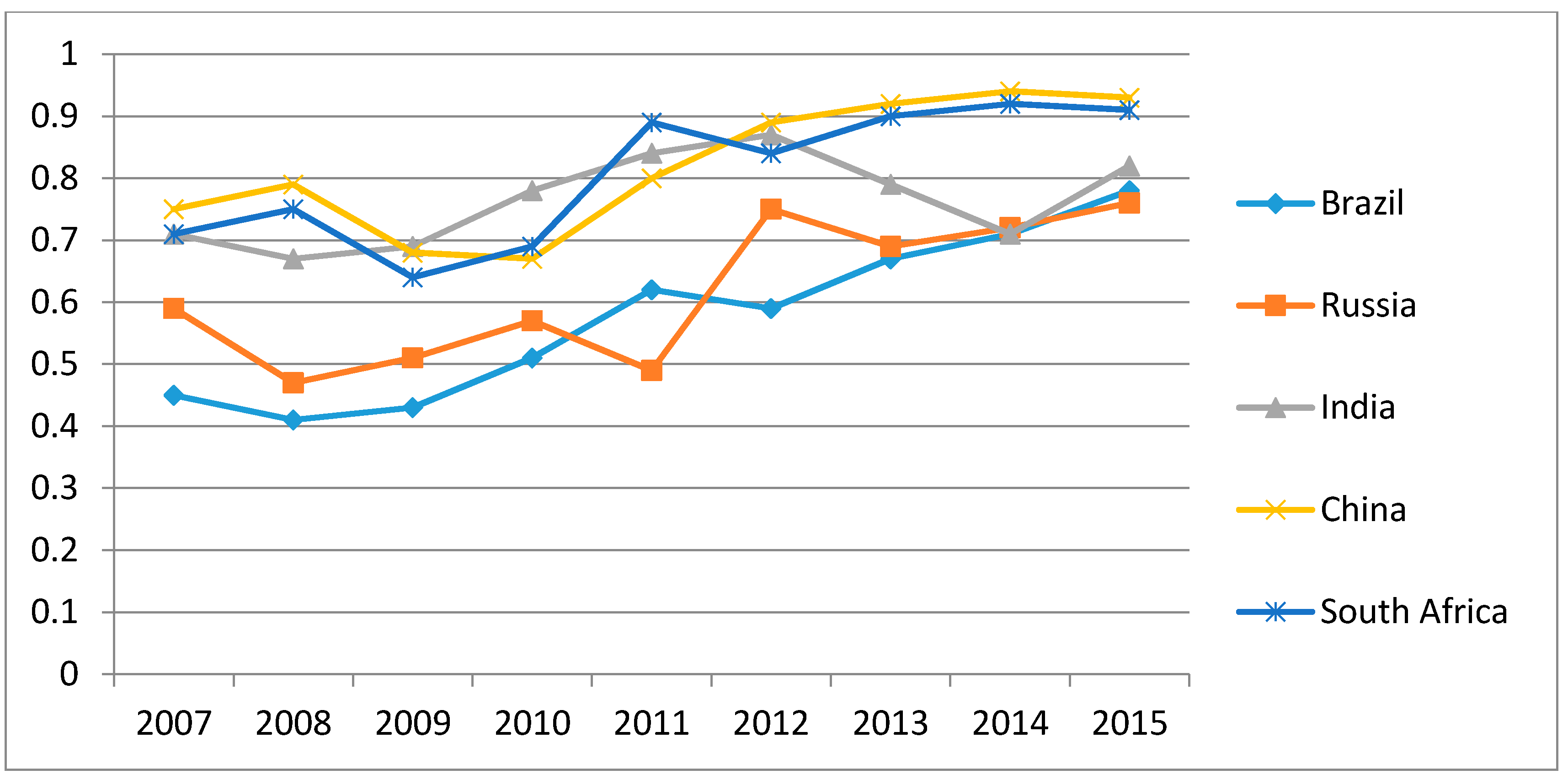
In this Equation (1), TC is the dependent variable and represents total cost. TC is defined as the sum of total interest and operating expenses. We follow the intermediation approach, and for inputs and outputs, we specify input prices (P) as the price of labor (PL), the price of fixed assets (PF), and the price of funds (PF)2, and outputs (Y) as total loans (TL) and other earning assets (OEA) (Zheng et al. 2017a). The graph below (Figure 1) shows the annual average cost efficiency scores of all banks within each sample country. With short-term fluctuations, the overall trend of bank efficiency in BRICS countries is upward sloping.

We measure several variables to control for bank- and country-level characteristics that can impact banks’ capital and the cost of financial intermediation in addition to the cost efficiency.

Our main measure of bank efficiency, COSTEFF, mainly focuses on bank efficiency in traditional lending activities. Therefore, we measure other aspects of bank efficiency with IMPLICOST and MANEFF variables. IMPLICOST equals the ratio of non-interest expenses to non-interest income and thus measures the bank efficiency in non-traditional income generation activities. MANEFF equals the ratio of earning assets to total assets. The higher the ratio, the greater the management efficiency is.

Bank size may affect the level of capital and the cost of financial intermediation. Large banks have several advantages as compared to small counterparts, including easy access to capital, higher diversification opportunities, and economies of scale (Zhang et al. 2008). Large banks can operate with lower capital ratios due to easy access to capital. Further, these banks can charge lower intermediation costs due to the economies of scale. Therefore, following recent studies (Ashraf et al. 2016a, 2017), we measure bank size, SIZE, as the natural logarithm of annual bank total assets.

Bank profits are a key indicator of bank overall health (Zheng et al. 2017a). Following Zheng et al. (2017a), we employ the ratio of pre-tax profit to total assets, PER, as a proxy for bank profits.

Higher leverage indicates higher financial risk and may impact bank behavior. We incorporate the debt to total assets ratio, LEV, to control for the effect of leverage.

Bank behavior might change during crisis periods. To control for this effect, we generate a crisis dummy variable, CRISISD, which equals 1 for the years 2007 to 2009 and 0 otherwise.

Similarly, explicit deposit insurance may generate moral hazard problems that lead banks to decrease bank equity or charge lower intermediation costs (Demirgüç-Kunt and Detragiache 2002; Demirgüç-Kunt and Huizinga 2004). In the presence of deposit insurance, bank equity acts as a put option on bank assets whose value can be increased either by reducing the equity or increasing the volatility of assets. Therefore, to control for this effect, we generate a deposit insurance dummy variable, DEPOD, which equals 1 for the countries with explicit deposit insurance and 0 for non-explicit deposit insurance countries.

Our sample includes banks from several countries which have different bank industry structures and macroeconomic conditions3. Therefore, in our empirical model, we include variables to control for the banking industry structure and macroeconomic conditions of the countries. We measure banking industry structure with the Hirschman-Herfindahl index (HHI). The HHI index is defined as the sum of squares of individual bank asset shares in the total banking sector assets for a country. This index has been widely used as a measure of market concentration where greater market concentration associated with lower competition among banks and vice versa (Islam and Nishiyama 2016). Two macroeconomic variables include INF and GDP. INF represents inflation and equals percentage change in annual average consumer prices. GDP represents GDP growth rates and equals annual percentage growth in gross domestic product of a country.

4. Empirical Methodology

We specify the following dynamic panel regression model for empirical analysis.

$${\mathrm{X}}_{\mathrm{ij},\mathrm{t}}=\mathrm{c}+{\mathsf{\delta }\mathrm{X}}_{\mathrm{ij},\mathrm{t}-1}+\mathsf{\lambda }\mathrm{COS}\mathrm{TEFFi},\mathrm{t}+{\displaystyle \sum }_{\mathrm{b}=1}^{\mathrm{B}}{\mathsf{\beta }}_{\mathrm{b}}{\mathrm{Y}}_{\mathrm{i},\mathrm{t}}^{\mathrm{b}}+{\displaystyle \sum }_{\mathrm{j}=1}^{\mathrm{J}}{\mathsf{\beta }}_{\mathrm{j}}{\mathrm{Y}}_{\mathrm{i},\mathrm{t}}^{\mathrm{j}}+{\displaystyle \sum }_{\mathrm{m}=1}^{\mathrm{M}}{\mathsf{\beta }}_{\mathrm{m}}{\mathrm{Y}}_{\mathrm{i},\mathrm{t}}^{\mathrm{m}}+{\in }_{\mathrm{i},\mathrm{t}}$$

(2)

Here, i, j, and t subscripts stand for bank, country, and year, respectively. X is the dependent variable. In different specifications, we use bank capital and the cost of financial intermediation as dependent variables. ${\mathrm{X}}_{\mathrm{ij},\mathrm{t}-1}$ is the one-period lag of the dependent variable. c is a constant term. δ denotes the speed of adjustment to equilibrium. COSTEFF is the main independent variable of interest. ${\mathrm{Y}}_{\mathrm{i},\mathrm{t}}$ with superscripts b, j, and m denote bank-specific, industry-specific, and macroeconomic determinants. ${\in }_{i,t}$ is the disturbance term. Bank-level variables represent bank implicit cost, management efficiency, size, profitability, leverage, and ownership structure. Bank industry level control variables measure banking industry structure and explicit deposit insurance. Country-level variables include inflation and gross domestic product.

Equation (2) includes a dynamic dependent variable, endogenous independent variables, and bank fixed-effects. For example, bank capital and the cost of financial intermediation may experience persistence over time due to regulations, lack of perfect competition among banks, and the opaque nature of banks. Further, COSTEFF is endogenous due to reverse causality from bank capital to efficiency. Several recent studies have found that capital requirements influence bank efficiency. Since bank cost-efficiency scores measure a bank’s relative efficiency as compared to a best-practice benchmark in transforming its inputs (e.g., deposits) to outputs (e.g., loans), bank capital can affect bank efficiency by influencing the mix of financing sources in bank capital structure and the allocation of bank assets portfolios. Finally, bank specific characteristics such as CEOs, boards, location, etc. remain unobserved bank-specific fixed-effects.

For a dynamic panel model with large N (1190 banks) and small T (9 years for this study) and having fixed-effects and endogenous variables, differenced (Arellano and Bond 1991) and system GMM estimators (Arellano and Bover 1995; Blundell and Bond 1998) can be used. System GMM provides more consistent estimates if the coefficient of lagged dependent variable, δ, is large, and in such cases the estimations with differenced GMM estimator are inefficient (Bond 2002). We observed that δ has fairly high values for all proxies of bank capital and the cost of financial intermediation, so we chose the two-step system GMM estimator to estimate Equation (2).

We perform an endogeneity test4 to determine whether the endogeneity exists between dependent variables and the main cost efficiency independent variable. Further, we employ finite-sample correction (Windmeijer 2005) to report standard errors of the two-step GMM results without which the standard errors tend to be severely downward biased. Moreover, we cluster standard errors at bank-level to control for the dependence of errors for a given bank over time. We also perform the test of non-stationary and the results are presented in Appendix A (

Table A1. Test of Non-Stationary.

Variables	χ2	p-value
Owners’ equity to total assets (Capital)	2392.35	0.0000
Net interest income to average earning assets (Cost of Inter.)	2246.51	0.0000
Non-interest expenses over non-interest income (Implicit cost)	3112.92	0.0000
Total earning assets to total assets (Management efficiency)	2160.52	0.0000
Logarithm of total assets (Size)	2164.88	0.0000
Pre-tax profit to total assets (Profitability)	1968.84	0.0000
Total debt to total assets (Leverage)	2019.27	0.0000
Herfindahl index	2782.63	0.0000
Inflation, consumer prices	984.222	0.0000
GDP growth (annual %)	2681.23	0.0000

Note: The table shows the Augmented Dickey–Fuller test Fisher-type (which does not require a panel to be balanced) results where the null of non-stationarity have been rejected for all the variables at 1% level of significance (all series are in Level except inflation). In case of dummy variables (all values lie between 0 and 1) and stochastic frontier scores (all values derived from log form, and the scores are in positive), this test is not required.

).

To further check the robustness of our results, we also estimated Equation (2) with other panel estimation techniques including the panel fixed-effects and pooled panel ordinary least squares (OLS) estimators.

5. Empirical Results

5.1. Summary Statistics

Table 2. Descriptive Statistics.

Variables	Mean	Median	Std. Deviation	N
Dependent variables
OETTA	0.185163	0.1387	0.144954	7887
NIM1	0.064447	0.056845	0.049201	7887
Main variable
COSTEFF	0.765698	0.622598	0.316985	7887
Independent variables Bank-specific
IMPLICOST	1.945009	1.279628	3.408559	7887
MANEFF	0.859718	0.879338	0.09839	7887
SIZE	5.920149	5.288606	2.64935	7887
CRISISD	0.191328	0	0.393371	7887
DEPOD	0.886649	1	0.317042	7887
OWND	0.678944	1	0.293484	7887
PER	0.048714	0.026484	0.154895	7887
LEV	0.712840	0.628749	0.138527	7887
Industry-specific
HHI	0.000633	2.35E-08	0.00517	7887
Macroeconomics-specific
INF	8.280194	7.812895	3.553881	7887
GDP	2.938296	4.264177	4.524021	7887

Source: authors’ calculations.

presents the summary statistics for the main variables. For more detail, Appendix B (

Table A2. Summary Statistics of Variables (Individual Country).

Variables	Brazil				Russia				India				China				South Africa
	Mean	Max	Min	S.D.	Mean	Max	Min	S.D.	Mean	Max	Min	S.D.	Mean	Max	Min	S.D.	Mean	Max	Min	S.D.
Dependent Variables:	0.16	0.86	−0.21	0.11	0.21	0.98	−1.19	0.15	0.09	0.75	0.03	0.07	0.09	0.78	−0.14	0.08	0.15	0.58	0.008	0.11
OETTA
NIM1	0.09	0.82	−0.38	0.11	0.07	0.58	−0.49	0.04	0.03	0.15	−0.48	0.03	0.03	0.07	0.005	0.01	0.07	0.37	0.01	0.07
Main Variable:
COSTEFF	0.64	0.89	0.21	0.31	0.69	0.92	0.16	0.42	0.75	0.94	0.12	0.64	0.84	0.91	0.38	0.21	0.81	0.95	0.31	0.19
Bank Level Variables:
IMPLICOST	3.53	43.49	−19.26	7.42	1.53	48.84	−16.0	2.03	2.06	27.33	−7.46	1.97	3.87	46.78	−16.09	5.81	1.62	8.91	0.54	1.18
MANEFF	0.87	1.02	0.34	0.11	0.86	1.00	0.08	0.10	0.90	1.00	0.23	0.07	0.85	1.00	0.42	0.06	0.81	0.98	0.19	0.17
SIZE	7.54	13.11	2.61	2.08	4.83	13.23	−0.94	1.84	9.10	13.01	3.64	1.67	10.11	15.05	4.69	1.93	8.08	12.21	3.44	2.70
OWND	0.62	1	0	0.23	0.69	1	0	0.34	0.71	1	0	0.32	0.59	1	0	0.24	0.66	1	0	0.28
PER	0.03	0.27	-0.16	0.11	0.02	0.19	-0.12	0.09	0.04	0.32	-0.08	0.13	0.06	0.21	-0.001	0.24	0.04	0.37	-0.18	0.17
LEV	0.76	0.94	0.12	0.16	0.69	0.73	0.10	0.09	0.62	0.79	0.34	0.07	0.54	0.68	0.27	0.06	0.79	0.91	0.11	0.15
CRISISD	0.19	1	0	0.39	0.20	1	0	0.40	0.20	1	0	0.40	0.08	1	0	0.27	0.18	1	0	0.39
Industry specific Variables:
Herfindahl index	0.002	0.19	0.000	0.01	0.0002	0.09	0.000	0.003	0.001	0.06	0.000	0.006	0.002	0.06	0.000	0.006	0.005	0.05	0.000	0.009
Macro−economic Variables:	5.96	9.03	3.64	1.36	9.24	15.52	5.08	3.30	8.76	11.99	5.87	2.10	2.69	5.86	−0.70	1.56	6.24	11.54	4.26	2.02
Inflation %
Gdp %	2.45	7.53	−3.85	3.27	1.97	8.54	−7.82	4.49	7.17	10.26	3.89	1.69	8.24	14.19	6.90	1.52	2.23	5.36	−1.54	1.60
Obs. (Banks)	686 (123)				5723 (793)				584 (90)				671 (154)				223 (30)

Notes: Max = Maximum Value, Min = Minimum Value, S.D. = Standard Deviation, Obs. = Observations.

) shows the summary statistics for each of the five sample countries separately. Mean value for equity to total assets ratio is 18.5 percent with a standard deviation of 14.5 percent. Mean value of net interest margins is 6.4 percent with a standard deviation of 4.9 percent. The mean value of cost-efficiency scores is 76.6 percent, showing that there is room for bank efficiency improvement in BRICS countries. Other variables also show considerable variation across mean values.

Table 3. Pearson’s Correlation Coefficient.

Variables	COSTEFF	IMPLICOST	MANEFF	SIZE	CRISISD	DEPOD	OWND	PER	LEV	HHI	INF	GDP
COSTEFF	1.000
IMPLICOST	0.079	1.000
MANEFF	0.110	0.026	1.000
SIZE	0.543	0.114	0.058	1.000
CRISISD	−0.065	−0.005	0.082	−0.111	1.000
DEPOD	−0.220	−0.143	0.076	−0.497	0.079	1.000
OWND	0.364	−0.241	−0.427	0.054	0.036	0.524	1.000
PER	0.285	0.541	0.0241	0.067	−0.385	−0.087	0.342	1.000
LEV	0.452	−0.035	0.098	0.514	0.069	0.075	−0.248	0.195	1.000
HHI	0.086	−0.008	0.024	0.307	−0.023	−0.119	0.078	−0.112	0.447	1.000
INF	−0.193	−0.132	−0.024	−0.376	0.292	0.473	−0.098	0.085	0.049	−0.063	1.000
GDP	0.211	0.104	0.113	0.295	0.414	−0.301	0.085	−0.025	0.168	0.042	−0.449	1.000

Source: Authors’ calculation, Total number of observations is 7887.

reports the pair-wise correlations between main variables. As shown, the correlations are not too high, suggesting that multicollinearity is less a concern in our multivariate analysis5.

5.2. Impact of Cost Efficiency on Bank Capital and the Cost of Financial Intermediation

Table 4. Determinants of Equity Capital and Banks’ Intermediation Cost.

Variables	(OETTA)	Robust S.E	(NIM1)	Robust S.E
Intercept	0.149 *** (8.18)	0.0182	0.006 * (1.98)	0.0030
OETTAt−1	0.702 *** (31.8)	0.0221
NIM1t−1			0.741 *** (16.38)	0.0452
COSTEFF	0.007 *** (5.59)	0.0012	−0.001 *** (−3.67)	0.0004
NIM1	0.190 *** (3.94)	0.0482
OETTA			0.031 *** (2.67)	0.0118
IMPLICOST			0.001 *** (3.24)	0.0002
MANEFF	−0.041 *** (−3.85)	0.0107
SIZE	−0.012 *** (−7.94)	0.0015
DEPOD	−0.029 *** (−4.19)	0.0068	0.004 *** (2.75)	0.0016
OWND	0.038 (1.59)	0.0239	0.054 *** (3.89)	0.0139
PER	0.001 ** (3.89)	0.0002	−0.021 *** (−6.89)	0.0030
LEV	−0.002 *** (−4.85)	0.0004	0.003 *** (3.57)	0.0008
HHI	0.875 *** (4.48)	0.1952	−0.022 (−0.41)	0.0540
INF	−0.0001 (−0.37)	0.0005	0.000 (0.05)	0.0002
GDP	−0.001 (−1.59)	0.0005
Time-dummies	Yes		Yes
Diagnostic Tests
Sargan test (p-value)	0.39		0.23
AR(1) (p-value)	−6.86 (0.00)		−5.97 (0.00)
AR(2) (p-value)	−1.09 (0.21)		−0.97 (0.34)
No. of Instruments	24		23
Econometric Tests
Endogeneity test (p-value)	0.01		0.00
LM serial correlation test (p-value)	0.00		0.00
White test (p-value)	0.00		0.00
Hausman F/R test (p-value)	1.00		1.00
Observations	7887		7887

Notes: Dependent variables are OETTA and NIM1. Higher values of these variables represent higher bank capital and higher cost of financial intermediation, respectively, and vice versa. Reported results are estimated with a two-step system GMM estimator. Heteroskedasticity-robust-statistics are reported in parentheses. The null hypothesis of the Sargan test is that instruments used are not correlated with residuals (over-identifying restrictions). Arellano–Bond order 1 (2) are tests for first (second) order correlation, asymptotically N (0, 1). These test the first-differenced residuals in the system GMM estimation. Cost efficiency is treated as an endogeneous variable. The null hypothesis of the endogeneity, serial correlation, and heteroskedasticity tests is that there is no such exist in the model and we reject the null hypothesis in all models. The null hypothesis of the fixed/random test is that there is a random effect among the variables in the model and we accept the null hypothesis. Detailed definitions of all varibles are given in Table 1. ***, ** and * indicate significance at the 1%, 5% and 10% levels, respectively.

reports main results where Equation (2) is estimated using two-step system GMM for each of two dependent variables of bank capital and the cost of financial intermediation.

As shown, COSTEFF enters positive and significant with OETTA, showing that cost-efficient banks have higher capital. This result is consistent with the expectation and confirms that costefficiency helps banks to accumulate capital through the profits. In second model, COSTEFF enters negative and significant with NIM1, showing that cost-efficient banks charge lower net interest margins. This result is also consistent with the expectation and confirms that cost efficiency helps banks transfer benefits to borrowers by charging lower margins on loans.

Results of control variables are also consistent with expectation. For example, IMPLICOST enters positive with NIM1, showing that banks inefficiency in non-lending activities let them to charge higher margins on their traditional activities. Size enters negative and significant with OETTA, showing that larger banks have several advantages and can operate with lower capital ratios. DEPOD also enters negative with OETTA, showing that deposit insurance generates moral hazard problems and let banks to decrease equity. DEPOD enters positive with NIM1, suggesting that explict deposit insurance widens the bank net interest margins. This result is expected to be driven through deposit and loan rates. On the one hand, deposit insurance provides a guarantee to depositors and lets them demand lower deposit rates on their deposits. On the other hand, moral hazard probems of deposit insurance encourage bankers to invest in risky assets which have higher interest rates.

PER enters postive with OETTA and negative with NIM1. The former result suggests that profitable can increase capital by retaining more profits, while the latter implies that more profitable banks are able to charge lower net interest margins.

LEV enters negative with OETTA and positive with NIM1, showing that banks with higher financial risk have low equity and charge higher net intersest margins.

Macroeconomic variables largly enter insignificant in both models. This result is not unsurprising given the small number of sample countries and short time period of sample.

Diagnostic tests of the two-step system GMM estimator confirms that the model has been appropriately specified. For example, lagged dependent variables enter with high coefficients showng high persistence. AR(1) and AR(2) test first-order and second-order serial correlations, respectively, in the equation in differences. Consistent with expectation, significant statistics of AR(1) confirms first-order serial correlation in residuals, while insignificant AR(2) statistics confirms that there is no second-order serial correlation in residuals.

Similarly, the number of instruments (23/24) is quite lower as compared to the number of banks (1190), showing that the results do not have the problem of instruments proliferation.

5.3. Robustness Tests: Alternative Proxies of Bank Capital and the Cost of Financial Intermediation

We perform several robustness tests to further confirm the main results. First in this section, we employ alternative proxies of both dependent variables. REG_CAP equals the bank regulatory capital to total assets ratio and is used as an altervitve proxy of bank capital. NIM2 equals the net interest income to average total assets ratio and is used as an altervative proxy of banks’ cost of financial intermediation. We estimate Equation (2) using these alternative proxies and report result in

Table 5. Determinants of Capital Ratio and Banks’ Intermediation Cost.

Variables	(REG_CAP)	Robust S.E	(NIM2)	Robust S.E
Intercept	0.156 *** (9.18)	0.0170	0.005 ** (2.29)	0.0022
REG_CAPt−1	0.741 *** (35.85)	0.0207
NIM2t−1			0.765 *** (16.24)	0.0471
COSTEFF	0.006 *** (5.64)	0.0011	−0.001 ** (−2.97)	0.0003
NIM2	0.242 *** (4.64)	0.0521
REG_CAP			0.023 ** (2.67)	0.0086
IMPLICOST			0.0001 ** (2.25)	0.0001
MANEFF	−0.053 *** (−5.75)	0.0092
SIZE	−0.011 *** (−7.67)	0.0014
DEPOD	−0.024 *** (−4.27)	0.0056	0.004 *** (2.94)	0.0013
OWND	0.042 (1.11)	0.0378	0.067 *** (4.11)	0.0163
PER	0.002 *** (4.21)	0.0005	−0.016 *** (−5.49)	0.0029
LEV	−0.003 *** (−3.98)	0.0008	0.002 *** (4.23)	0.0005
HHI	0.880 *** (4.67)	0.1885	−0.022 (−0.37)	0.0595
INF	0.000 (−0.27)	0.0007	0.000 (−0.31)	0.0002
GDP	−0.001 (−1.69)	0.0005
Time-dummies	Yes		Yes
Diagnostic Tests
Sargan test (p-value)	0.47		0.27
AR(1) (p-value)	−6.97 (0.00)		−6.31 (0.00)
AR(2) (p-value)	−1.16 (0.18)		−1.03 (0.23)
No. of Instruments	24		23
Econometric Tests
Endogeneity test (p-value)	0.03		0.00
LM serial correlation test (p-value)	0.00		0.00
White test (p-value)	0.00		0.00
Hausman F/R test (p-value)	1.00		1.00
Observations	7887		7887

Notes: Dependent variables are REG_CAP and NIM2. Higher values of these variables represent higher bank regulatory capital and higher cost of financial intermediation, respectively, and vice versa. Reported results are estimated with a two-step system GMM estimator. Heteroskedasticity-robust-statistics are reported in parentheses. The null hypothesis of the Sargan test is that the instruments used are not correlated with residuals (over-identifying restrictions). Arellano–Bond order 1 (2) are tests for first (second) order correlation, asymptotically N (0, 1). These test the first-differenced residuals in the system GMM estimation. Costefficiency is treated as endogeneious variable. The null hypothesis of the endogeneity, serial correlation, and heteroskedasticity tests is that there is no such exist in the model and we reject the null hypothesis in all models. The null hypothesis of the fixed/random test is that there is a random effect among the variables in the model and we accept the null hypothesis. Detailed definitions of all varibles are given in Table 1. *** and ** indicate significance at the 1% and 5% levels, respectively.

. As shown, the results of COSTEFF remains same: it enters postive and significant with REG_CAP and negative and significant with NIM2. These results again confirm our main results. Results of other control variables largely remain same as Table 4.

5.4. Robustness Tests: Alternative Estimation Methods and Dropping Russian Banks

As another robustness test, we estimate both specifications of Table 4 with panel fixed-effects and pooled panel OLS estimators. As shown in

Table 6. Determinants of Equity Capital and Banks’ Intermediation Cost.

Variables	Fixed Effect Estimation		Pooled Panel OLS Estimation		Dropped Russia
	(OETTA)	(NIM1)	(OETTA)	(NIM1)	(OETTA)	(NIM1)
	(1)	(2)	(3)	(4)	(5)	(6)
Intercept	0.623 ***	0.047 ***	0.340 ***	0.041 ***	0.143 ***	0.033 ***
	(0.00)	(0.00)	(0.00)	(0.00)	(0.00)	(0.00)
COSTEFF	0.022 ***	−0.005 **	0.033 ***	−0.005 ***	0.006 ***	−0.005 ***
	(0.00)	(0.01)	(0.00)	(0.00)	(0.00)	(0.00)
NIM1	0.432 ***		0.445 ***		0.354 ***
	(0.00)		(0.00)		(0.00)
OETTA		0.065 ***		0.033 ***		0.311 ***
		(0.00)		(0.00)		(0.00)
IMPLICOST		0.002 ***		0.001 ***	0.004 ***
		(0.00)		(0.00)	(0.00)
MANEFF	−0.057 ***		−0.013			−0.240 ***
	(0.00)		(0.16)			(0.00)
SIZE	−0.066 ***		−0.053 ***			−0.003 ***
	(0.00)		(0.00)			(0.00)
DEPOD	−0.016 ***	0.003 ***	−0.063 ***	0.013 ***	−0.062 ***	0.023 ***
	(0.00)	(0.00)	(0.00)	(0.00)	(0.00)	(0.00)
OWND	0.002	0.053 ***	0.011*	0.049 ***	0.014	0.023 ***
	(0.19)	(0.00)	(0.09)	(0.00)	(0.42)	(0.00)
PER	0.001 ***	−0.014 ***	0.003 ***	−0.019 ***	0.0001 ***	−0.017 ***
	(0.00)	(0.00)	(0.00)	(0.00)	(0.00)	(0.00)
LEV	−0.004 ***	0.001 ***	−0.002 ***	0.005 ***	−0.009 ***	0.007 ***
	(0.00)	(0.00)	(0.00)	(0.00)	(0.00)	(0.00)
HHI	−0.213	0.018	1.438 ***	−0.019	−0.282	−0.005
	(0.26)	(0.38)	(0.00)	(0.17)	(0.42)	(0.31)
INF	−0.004 ***	0.001 *	−0.001 *	0.005 ***	−0.002 **	0.0001
	(0.00)	(0.06)	(0.05)	(0.00)	(0.03)	(0.27)
GDP	0.0001		−0.0001		0.0005
	(0.19)		(0.34)		(0.21)
Time-dummies	No	No	Yes	Yes	Yes	Yes
Adjusted R2	72.96%	53.67%	76.28%	59.84%	63.27%	47.18%
F-statistics (p-value)	519.57 (0.00)	198.84 (0.00)	589.79 (0.00)	293.84 (0.00)
Wald test (p-value)					310.24 (0.00)	283.84 (0.00)
Observations	7887	7887	7887	7887	2164	2164

Notes: Dependent variables are OETTA and NIM1. Higher values of these variables represent higher bank capital and higher cost of financial intermediation, respectively, and vice versa. The estimation methods are fixed-effects, the pooled panel OLS, and random effect estimation (dropped Russia). p-values are presented in parentheses. The standard errors for regression coefficients are clustered at bank-level to control for the dependence of errors for a given bank over time. Detailed definitions of all varibles are given in Table 1. ***, ** and * indicate significance at the 1%, 5% and 10% levels, respectively.

, the results remain the same; COSTEFF enters postive and significant with OETTA, and negative and significant with NIM1. Results for other control variables also largely remain the same. These results again confirm that our main results in Table 4 are not biased due to two-step GMM estimations.

Further, in a multicountry study, the econometric results may be biased due to very high number of observations from a specific country. To eliminate this concern, we drop all observations (which constitute 73% of the sample) for Russian banks and re-estimate both specifications of Table 4. As shown in last two models of Table 6, the results of COSTEFF variable remain same. These results confirm that our main results are not driven by the banks from a specific country.

5.5. Robustness Tests: Balanced Panel Data Analysis

Our main dataset is an unbalanced panel where different banks have different observations over sample period. To eliminate the concern that main results are not biased due to some banks with more yearly observations, we consider only those banks with all yearly observations over sample period of 2007–2015. After converting the dataset in a balanced panel, we re-estimate both main models using two-step system GMM. As shown in

Table 7. Impact of Cost Efficiency on Bank Capital and Intermediation Cost (Balanced Panel Data).

Variables	(OETTA)	Robust S.E	(NIM1)	Robust S.E
Intercept	0.094 *** (5.57)	0.0169	0.021 *** (5.98)	0.0035
OETTAt−1	0.507 *** (18.64)	0.0272
NIM1t−1			0.532 *** (11.29)	0.0471
COSTEFF	0.003 *** (4.67)	0.0006	−0.003 *** (−4.10)	0.0007
NIM1	0.241 ** (2.27)	0.1062
OETTA			0.065 ** (2.38)	0.0273
IMPLICOST			0.005 ** (2.31)	0.0022
MANEFF	−0.027 ** (−2.20)	0.0123
SIZE	−0.031 *** (−6.87)	0.0045
DEPOD	−0.013 *** (−2.95)	0.0044	0.002 ** (2.14)	0.0009
OWND	0.027(0.24)	0.1125	0.092 *** (5.34)	0.0172
PER	0.003 *** (3.36)	0.0009	−0.034 *** (−7.37)	0.0046
LEV	−0.001 ** (−2.24)	0.0004	0.006 *** (3.92)	0.0015
HHI	0.354 ** (2.68)	0.1321	−0.037 * (−1.41)	0.0262
INF	−0.003 (−1.10)	0.0027	0.002 (0.38)	0.0053
GDP	−0.006 ** (−2.67)	0.0022
Time-dummies	Yes		Yes
Diagnostic Tests
Sargan test (p-value)	0.27		0.11
AR(1) (p-value)	−2.67 (0.00)		−2.29 (0.01)
AR(2) (p-value)	−0.58 (0.63)		−0.61 (0.56)
No. of Instruments	24		23
Observations	2583		2583
No. of bank	287		287

Notes: Dependent variables are OETTA and NIM1. Higher values of these variables represent higher bank capital and higher cost of financial intermediation, respectively, and vice versa. Reported results are estimated with a two-step system GMM estimator. Heteroskedasticity-robust-statistics are reported in parentheses. The null hypothesis of the Sargan test is that the instruments used are not correlated with residuals (over-identifying restrictions). Arellano–Bond order 1 (2) are tests for first (second) order correlation, asymptotically N (0, 1). These test the first-differenced residuals in the system GMM estimation. Cost efficiency is treated as an endogenous variable. Detailed definitions of all varibles are given in Table 1. ***, ** and * indicate significance at the 1%, 5% and 10% levels, respectively.

, COSTEFF enters positive and significant with OETTA, and negative and significant with NIM1. These results confirm that our main results are not biased due to the unbalanced nature of the dataset.

5.6. Country-Wise Regression Results

Next, we examine the impact of cost efficiency on bank capital and the cost of financial intermediation for each of the five sample countries. For doing so, we distribute banks of the main sample into their respective countries, then we estimate both specifications of Table 4 for the banks of each country.

Table 8. Impact of Cost Efficiency on Bank Capital (Country-Wise Regressions).

Variables	Brazil	Russia	India	China	South Africa
	(OETTA)	(OETTA)	(OETTA)	(OETTA)	(OETTA)
Intercept	0.112 *** (2.68)	0.157 *** (9.82)	0.042**(2.89)	0.176 *** (7.28)	0.056 ** (2.25)
OETTAt−1	0.682 *** (8.38)	0.864 *** (25.34)	0.761 *** (7.68)	0.569 *** (11.36)	0.724 *** (13.18)
COSTEFF	−0.004 ** (−2.72)	0.032 *** (6.67)	0.002 *** (−2.89)	0.001*(1.49)	−0.003 *** (−5.39)
NIM1	−0.124 *** (−3.51)	−0.031(−0.34)	−0.357**(−2.28)	−0.637 *** (−5.84)	0.007(0.09)
MANEFF	0.034 (0.54)	−0.063 *** (−4.33)	−0.032 (−1.21)	−0.057 ** (−2.34)	−0.038 (−1.23)
SIZE	−0.007 *** (−4.57)	−0.014 *** (−9.37)	−0.002 ** (−2.59)	−0.004 *** (−4.81)	0.001 (0.87)
OWND	0.042(0.79)	0.016(1.02)	0.024(1.39)	0.019(0.92)	0.034(0.38)
PER	0.024 ***(5.39)	0.001 **(2.65)	0.027 *(1.67)	0.015 ***(4.68)	0.037 *(1.69)
LEV	−0.002(−1.24)	−0.012 **(−2.36)	−0.039 ***(−5.34)	−0.24 **(−2.14)	−0.051(−0.49)
HHI	0.192 (1.10)	0.934 *** (8.27)	−0.031 (−0.28)	0.341 ** (2.27)	−0.257 * (−1.98)
GDP	0.002 ** (2.58)	−0.003 *** (−2.93)	0.008 *** (3.48)	−0.003 *** (−6.18)	0.0001 (0.27)
Time-dummies	Yes	Yes	Yes	Yes	Yes
Adjusted R2	57.54%	63.51%	80.29%	87.17%	79.61%
Sargan test (p-value)	0.24	0.13	0.47	0.28	0.09
AR(1) (p-value)	−3.68 (0.00)	−4.96 (0.00)	−3.72 (0.00)	−4.01 (0.00)	−2.23 (0.01)
AR(2) (p-value)	−1.12 (0.29)	−1.43 (0.15)	−0.92 (0.41)	−1.16 (0.25)	−1.47 (0.12)
Instruments	24	25	27	23	24
Observations	686	5723	584	671	223
No. of Banks	123	793	90	154	30

Note: Dependent variable is OETTA in all models where higher values of this variable represent higher bank capital, and vice versa. Reported results are estimated with a two-step system GMM estimator. Heteroskedasticity-robust-statistics are reported in parentheses. The null hypothesis of the Sargan test is that the instruments used are not correlated with residuals (over-identifying restrictions). Arellano–Bond order 1 (2) are tests for first (second) order correlation, asymptotically N (0, 1). These test the first-differenced residuals in the system GMM estimation. Cost efficiency is treated as an endogenous variable. Detailed definitions of all varibles are given in Table 1. ***, ** and * indicate significance at the 1%, 5% and 10% levels, respectively.

reports results when bank capital is used as dependent variable. As shown, cost efficiency has a significant positive impact on bank capital in Russia, India, and China. Surprisingly, cost efficiency and bank capital show a negtive relation for Brazilian and South African banks. These country-level results show that our main results are driven by heavy weight members of BRICS block such as the China and India.

Table 9. Impact of Cost Efficiency on the Banks’ Cost of Financial Intermediation (Country-Wise Regressions).

Variables	Brazil	Russia	India	China	South Africa
	(NIM1)	(NIM1)	(NIM1)	(NIM1)	(NIM1)
Intercept	0.043 *** (3.38)	0.005 ** (2.68)	0.016 *** (3.55)	0.0051 (0.75)	0.0194 ** (2.68)
NIM1t−1	0.547 *** (10.64)	0.482 *** (22.61)	0.161 *** (4.89)	0.758 *** (26.54)	0.864 *** (12.19)
COSTEFF	−0.006 ** (−2.37)	−0.0005 * (−1.82)	−0.002 ** (−2.79)	−0.0002 ** (−2.73)	−0.004 ** (−2.81)
OETTA	−0.046 ** (−2.79)	0.027 ** (2.61)	0.164 ** (2.92)	−0.003 (−0.32)	−0.017 * (−1.73)
IMPLICOST	0.0003 (0.67)	0.0006 (1.43)	0.0004 *** (4.27)	5.57E−04 *** (6.89)	−0.0006 (−1.15)
OWND	0.065 ***(6.37)	0.028 ***(3.98)	0.038 ***(5.87)	0.053 ***(6.59)	0.087 ***(3.62)
PER	−0.012**(−2.96)	−0.034 ***(−6.57)	−0.059**(−2.25)	−0.039 ***(−4.68)	−0.072(−1.24)
LEV	0.004 ***(3.92)	0.0001*(1.94)	0.003 ***(6.37)	0.0002*(1.82)	0.005 ***(3.43)
HHI	−0.181 *** (−3.58)	−0.015 (−0.49)	−0.167 *** (−3.57)	−0.004 (−0.64)	−0.264 * (−1.69)
INF	−0.002 (−1.27)	−0.0002 (−0.39)	0.0003 * (1.93)	0.003 *** (5.37)	−0.002 (−0.79)
Time-dummies	Yes	Yes	Yes	Yes	Yes
Adjusted R2	59.34%	64.81%	19.87%	77.83%	89.68%
Sargan test (p-value)	0.16	0.48	0.28	0.37	0.13
AR(1) (p-value)	−4.42 (0.00)	−5.87 (0.00)	−4.53 (0.00)	−4.69 (0.00)	−2.96 (0.00)
AR(2) (p-value)	−1.01 (0.20)	−1.31 (0.14)	−1.26 (0.16)	−1.39 (0.11)	−1.32 (0.14)
Instruments	23	24	26	22	23
Observations	686	5723	584	671	223
No. of Banks	123	793	90	154	30

Note: Dependent variable is NIM1 in all models where higher values of NIM1 represent higher cost of financial intermediation, and vice versa. Reported results are estimated with a two-step system GMM estimator. Heteroskedasticity-robust-statistics are reported in parentheses. The null hypothesis of the Sargan test is that the instruments used are not correlated with residuals (over-identifying restrictions). Arellano–Bond order 1 (2) are tests for first (second) order correlation, asymptotically N (0, 1). These test the first-differenced residuals in the system GMM estimation. Cost efficiency is treated as an endogenous variable. Detailed definitions of all varibles are given in Table 1. ***, ** and * indicate significance at the 1%, 5% and 10% levels, respectively.

reports results when banks’ cost of financial intermediation is used as dependent variable. Consistent with main results, the cost efficiency has a negative impact on banks’ cost of financial intermediation in all sample countries. Results of other variables also largely remain same.

5.7. Crisis Period Analysis: Expanded Sample (2000–2015)

Since BRICS block banking sectors had minimal adverse effects during the global financial crisis of 2007–2009 (Jacobs and Van Rossem 2014), we next examine whether bank efficiency had a role in bank safety in these countries during the crisis. For doing so, we employ a crisis period dummy variable to examine the impact of the global financial crisis (GFC) on bank capital and the cost of financial intermediation. CRISISD equals 1 for the global financial crisis years of 2007–2009 and 0 otherwise. To clearly delineate non-crisis and crisis period effects, we extend our sample period from the year 2000 to 2015. We also introduce an interaction term of COSTEFF and CRISISD in regression to examine the marginal effect of bank efficiency on capital and financial intermediation costs during the crisis.

As shown in

Table 10. Impact of Cost Efficiency on Bank Capital and the Cost of Financial Intermediation.

Variables	(OETTA)	Robust S.E	(NIM1)	Robust S.E
Intercept	0.218 *** (8.19)	0.0266	0.010 ** (2.99)	0.0033
COSTEFF	0.005 *** (5.79)	0.0009	−0.003 *** (−3.10)	0.0010
CRISISD	0.009 *** (3.29)	0.0027	0.007 *** (8.74)	0.0008
COSTEFF*CRISISD	0.004 ** (2.97)	0.0013	−0.002 *** (5.89)	0.0003
NIM1	0.234 *** (3.18)	0.0736
OETTA			0.068 *** (3.83)	0.0178
Other control variables	Yes		Yes
Year fixed effect dummies	Yes		Yes
Adjusted R2	81.27%		63.49%
F-statistics (p-value)	2198.21 (0.00)		2351.57 (0.00)
Observations	9483		9483

Notes: Dependent variables are OETTA and NIM1. Higher values of these variables represent the higher equity in the capital structure and higher cost of financial intermediation and vice versa. The estimation method is the Pooled Panel OLS estimator. Heteroskedasticity-robust-statistics are in parentheses. Detailed definitions of all varibles are given in Table 1. *** and ** indicate significance at 1% and 5% levels, respectively.

, the results of COSTEFF with OETTA and NIM1 remain same even for the extended sample period. CRISISD enters positive and significant with both OETTA and NIM1. These results suggest that bank capital was relatively higher during the crisis years in BRICS countries. This shows that the capital position of BRICS banks was sound and is consistent with the real-world situation that banking sectors in BRICS countries largely remain isolated from the negative effects of the financial crisis. On the other hand, the positive association of CRISISD with NIM1 suggests that banks priced higher risks associated with weak economic conditions during crisis period and thus increased interest margins. In the first model, the interaction term, COSTEFF*CRISISD, enters positive and significant with bank capital, showing that more efficient banks have relatively higher capital during the crisis. In the second model, the interaction term enters negative and significant with banks’ financial intermediation cost, suggesting that more efficient banks did not charge higher financial intermediation costs during the crisis. Overall, these results suggest that cost efficiency helped banks to maintain higher capital and not charge higher intermediation costs during the crisis, and thus the impact implies a marginal beneficial impact of bank efficiency during the crisis.

6. Conclusions

This paper aims to examine the impact of bank cost efficiency on bank capital and the cost of financial intermediation.

Employing a panel dataset of 1190 banks from five BRICS countries over the period 2007–2015, we find that cost efficiency has a significant positive impact on bank capital and a significant negative impact on banks’ cost of financial intermediation. These results are robust to the use of alternative proxies of bank capital and the cost of financial intermediation, alternative estimation methods, and alternative sample compositions.

Further, we test the influence of the recent global financial crisis on bank capital and financial intermediation costs with the extended sample from the year 2000 to 2015. We observe that bank equity ratios in BRICS countries did not deteriorate during the crisis period, suggesting that the crisis had less impact on bank capital in these countries. We also find that bank net interest margins widened during the crisis period.

With the interaction of bank cost efficiency and financial crisis variables, we further observe that cost efficiency helped banks to maintain higher capital and not charge higher intermediation costs during the crisis.

Since bank capital can absorb losses in distress and banks with higher capital are considered safer, similarly, lower intermediation costs result in cheap financing for borrowers which is considered beneficial for real economy. Therefore, our results in this study imply beneficial impact of bank efficiency for bank stability and real economy. We suggest that BRICS block countries should continue or even accelerate financial sector reforms that encourage bank efficiency.

References

1. Admati, Anat R., and Martin Hellwig. 2013. The Bankers’ New Clothes: What’s Wrong with Banking and What to Do about It. Princeton: Princeton University Press. [Google Scholar]
2. Agapova, Anna, and James E. McNulty. 2016. Interest rate spreads and banking system efficiency: General considerations with an application to the transition economies of central and eastern europe. International Review of Financial Analysis 47: 154–65. [Google Scholar] [CrossRef]
3. Alam, Nafis. 2012. The impact of regulatory and supervisory structures on bank risk and efficiency: Evidence from dual banking system. Asian Journal of Finance & Accounting 4: 216–44. [Google Scholar]
4. Arellano, Manuel, and Stephen Bond. 1991. Some tests of specification for panel data: Monte carlo evidence and an application to employment equations. The Review of Economic Studies 58: 277–97. [Google Scholar] [CrossRef]
5. Arellano, Manuel, and Olympia Bover. 1995. Another look at the instrumental variable estimation of error-components models. Journal of Econometrics 68: 29–51. [Google Scholar] [CrossRef]
6. Ashraf, Badar Nadeem. 2016. Political Institutions, Political Pressure and State-Owned Banks’ Lending and Performance: Evidence from Developing Countries. Available online: https://ssrn.com/abstract=2761726 (accessed on 25 November 2017).
7. Ashraf, Badar Nadeem. 2017a. Do trade and financial openness matter for financial development? Bank-level evidence from emerging market economies. Research in International Business and Finance. [Google Scholar] [CrossRef]
8. Ashraf, Badar Nadeem. 2017b. Political institutions and bank risk-taking behavior. Journal of Financial Stability 29: 13–35. [Google Scholar] [CrossRef]
9. Ashraf, Badar Nadeem, and Sidra Arshad. 2017. Foreign bank subsidiaries’ risk-taking behavior: Impact of home and host country national culture. Research in International Business and Finance 41: 318–35. [Google Scholar] [CrossRef]
10. Ashraf, Badar Nadeem, and Changjun Zheng. 2015. Shareholder protection, creditor rights and bank dividend policies. China Finance Review International 5: 161–86. [Google Scholar] [CrossRef]
11. Ashraf, Badar Nadeem, Bushra Bibi, and Changjun Zheng. 2016a. How to regulate bank dividends? Is capital regulation an answer? Economic Modelling 57: 281–93. [Google Scholar] [CrossRef]
12. Ashraf, Badar Nadeem, Changjun Zheng, and Sidra Arshad. 2016b. Effects of national culture on bank risk-taking behavior. Research in International Business and Finance 37: 309–26. [Google Scholar] [CrossRef]
13. Ashraf, Badar Nadeem, Sidra Arshad, and Yuancheng Hu. 2016c. Capital regulation and bank risk-taking behavior: Evidence from pakistan. International Journal of Financial Studies 4: 16. [Google Scholar] [CrossRef]
14. Ashraf, Badar Nadeem, Sidra Arshad, and Liang Yan. 2017. Trade openness and bank risk-taking behavior: Evidence from emerging economies. Journal of Risk and Financial Management 10: 15. [Google Scholar] [CrossRef]
15. Ataullah, Ali, and Hang Le. 2006. Economic reforms and bank efficiency in developing countries: The case of the indian banking industry. Applied Financial Economics 16: 653–63. [Google Scholar] [CrossRef]
16. Berger, Allen N., and Emilia Bonaccorsi di Patti. 2006. Capital structure and firm performance: A new approach to testing agency theory and an application to the banking industry. Journal of Banking and Finance 30: 1065–102. [Google Scholar] [CrossRef]
17. Blundell, Richard, and Stephen Bond. 1998. Initial conditions and moment restrictions in dynamic panel data models. Journal of Econometrics 87: 115–43. [Google Scholar] [CrossRef]
18. Bond, Stephen. 2002. Dynamic panel data models: A guide to micro data methods and practice. Portuguese Economic Journal 1: 141–62. [Google Scholar] [CrossRef]
19. Carvallo, Oscar, and Adnan Kasman. 2017. Convergence in bank performance: Evidence from latin american banking. The North American Journal of Economics and Finance 39: 127–42. [Google Scholar] [CrossRef]
20. Demirgüç-Kunt, Asli, and Enrica Detragiache. 2002. Does deposit insurance increase banking system stability? An empirical investigation. Journal of Monetary Economics 49: 1373–406. [Google Scholar] [CrossRef]
21. Demirgüç-Kunt, Asli, and Harry Huizinga. 2004. Market discipline and deposit insurance. Journal of Monetary Economics 51: 375–99. [Google Scholar] [CrossRef]
22. Demirgüç-Kunt, Asli, Baybars Karacaovali, and Luc Laeven. 2005. Deposit insurance around the world: A comprehensive database. World Bank Policy Research Working Paper. [Google Scholar] [CrossRef]
23. Fiordelisi, Franco, David Marques-Ibanez, and Philip Molyneux. 2011. Efficiency and risk in european banking. Journal of Banking & Finance 35: 1315–26. [Google Scholar]
24. Fonseca, Ana Rosa, and Francisco González. 2010. How bank capital buffers vary across countries: The influence of cost of deposits, market power and bank regulation. Journal of Banking and Finance 34: 892–902. [Google Scholar] [CrossRef]
25. Gropp, Reint, and Florian Heider. 2010. The determinants of bank capital structure. Review of Finance 14: 587–622. [Google Scholar] [CrossRef]
26. Gujarati, Damodar N. 2007. Sangeetha (2007) Basic Econometrics. New Delhi: Tata McGraw Hill Publishing Company Limited, vol. 110, pp. 451–52. [Google Scholar]
27. Houston, Joel F., Chen Lin, Ping Lin, and Yue Ma. 2010. Creditor rights, information sharing, and bank risk taking. Journal of Financial Economics 96: 485–512. [Google Scholar] [CrossRef]
28. Huang, Tai-Hsin, Chung-I Lin, and Kuan-Chen Chen. 2017. Evaluating efficiencies of Chinese commercial banks in the context of stochastic multistage technologies. Pacific-Basin Finance Journal 41: 93–110. [Google Scholar] [CrossRef]
29. IIF. 2011. The Cumulative Impact on the Global Economy of Changes in the Financial Regulatory Framework. Washington: Institute of International Finance. [Google Scholar]
30. Islam, Md Shahidul, and Shin-Ichi Nishiyama. 2016. The determinants of bank net interest margins: A panel evidence from south asian countries. Research in International Business and Finance 37: 501–14. [Google Scholar] [CrossRef]
31. Jacobs, Lindsay Marie, and Ronan Van Rossem. 2014. The bric phantom: A comparative analysis of the brics as a category of rising powers. Journal of Policy Modeling 36: S47–S66. [Google Scholar] [CrossRef]
32. Kanagaretnam, Kiridaran, Lim Chee Yeow, and Gerald J Lobo. 2014. Influence of national culture on accounting conservatism and risk-taking in the banking industry. Accounting Review 89: 1115–49. [Google Scholar] [CrossRef]
33. Kumbhakar, Subal C., and C. A. Knox Lovell. 2003. Stochastic Frontier Analysis. Cambridge: Cambridge University Press. [Google Scholar]
34. Manlagnit, Maria Chelo V. 2015. Basel regulations and banks’ efficiency: The case of the philippines. Journal of Asian Economics 39: 72–85. [Google Scholar] [CrossRef]
35. Pasiouras, Fotios. 2008. International evidence on the impact of regulations and supervision on banks’ technical efficiency: An application of two-stage data envelopment analysis. Review of Quantitative Finance and Accounting 30: 187–223. [Google Scholar] [CrossRef]
36. Pasiouras, Fotios, Sailesh Tanna, and Constantin Zopounidis. 2009. The impact of banking regulations on banks’ cost and profit efficiency: Cross-country evidence. International Review of Financial Analysis 18: 294–302. [Google Scholar] [CrossRef]
37. Rahman, Mohammed Mizanur, Changjun Zheng, Badar Nadeem Ashraf, and Mohammad Morshedur Rahman. 2017. Capital requirements, the cost of financial intermediation and risk-taking: Empirical evidence from bangladesh. Research in International Business and Finance. in press. [Google Scholar] [CrossRef]
38. Slovik, Patrick, and Boris Cournède. 2011. Macroeconomic Impact of Basel III. OECD Economics Department Working Papers, No. 844. Available online: https://ssrn.com/abstract=2650033 or http://dx.doi.org/10.2139/ssrn.2650033 (accessed on 2 November 2017).
39. Wanke, Peter, Carlos P. Barros, and João R. Faria. 2015. Financial distress drivers in brazilian banks: A dynamic slacks approach. European Journal of Operational Research 240: 258–68. [Google Scholar] [CrossRef]
40. Wanke, Peter, Abul Kalam Azad, and Ali Emrouznejad. Efficiency in brics banking under data vagueness: A two-stage fuzzy approach. Global Finance Journal. [CrossRef]
41. Windmeijer, Frank. 2005. A finite sample correction for the variance of linear efficient two-step gmm estimators. Journal of Econometrics 126: 25–51. [Google Scholar] [CrossRef]
42. Wong, T. C., Tom Fong, KaFai Li, and Henry Choi. 2010. An Assessment of the Long-Term Economic Impact of the New Regulatory Reform on Hong Kong. Hong Kong Monetary Authority Research Note No. 05/2010. Available online: https://ssrn.com/abstract=1768642 or http://dx.doi.org/10.2139/ssrn.1768642 (accessed on 2 November 2017).
43. Zhang, Zong-yi, Wu Jun, and Qiong-fang Liu. 2008. Impacts of capital adequacy regulation on risk-taking behaviors of banking. Systems Engineering-Theory & Practice 28: 183–89. [Google Scholar]
44. Zheng, Changjun, and Badar Nadeem Ashraf. 2014. National culture and dividend policy: International evidence from banking. Journal of Behavioral and Experimental Finance 3: 22–40. [Google Scholar] [CrossRef]
45. Zheng, Changjun, Mohammed Mizanur Rahman, Munni Begum, and Badar Nadeem Ashraf. 2017a. Capital regulation, the cost of financial intermediation and bank profitability: Evidence from bangladesh. Journal of Risk and Financial Management 10: 9. [Google Scholar] [CrossRef]
46. Zheng, Changjun, Syed Moudud-Ul-Huq, Mohammad Morshedur Rahman, and Badar Nadeem Ashraf. 2017b. Does the ownership structure matter for banks’ capital regulation and risk-taking behavior? Empirical evidence from a developing country. Research in International Business and Finance 42: 404–21. [Google Scholar] [CrossRef]
1
2
Price of labor = personal expenses/total assets, price of fixed assets = Depreciation cost/total assets, price of fund = total interest expenses/total deposit (Fiordelisi et al. 2011).
3
Recent literature reports that banking practices in different countries are influenced by the national culture (Zheng and Ashraf 2014; Ashraf et al. 2016b; Kanagaretnam et al. 2014; Ashraf and Arshad 2017), legal institutions (Houston et al. 2010; Ashraf and Zheng 2015) and political institutions (Ashraf 2016, 2017b). Therefore, it is important to include country-level variables in analysis.
4
The null of endogeneity test is that there is no endogeneity problem and we reject the null in both cases, for bank capital and cost efficiency, and banks’ cost of financial intermediation and cost efficiency.
5
Gujarati (2007) indicates that multicollinearity is a serious problem if the correlation coefficient between two independent variables is above 0.80, which is not the case here.
Figure 1. Average cost-efficiency scores of banks within each sample country.
Ijfs 05 00032 g001