Cross-Quantile Dependence Between Green Bonds and Financial Markets: A Cross-Quantilogram Approach

Abstract

The opportunities in green investment have propelled the green bond market at a time when climate change has emerged as a critical issue. As more investors express a preference for environmentally responsible investments, the popularity of green bonds remains high. Such considerations motivate the exploration of the relationship between these instruments and different assets to better appreciate their potential benefits. This paper examines the relationship between green bonds and various financial markets, including conventional bonds, equities, oil, and clean energy stocks, using daily return data from July 2014 to October 2024. Hence, the cross-quantilogram approach is employed to explore how Economic Policy Uncertainty (EPU) and Financial Market Uncertainty (VIX) influence these dependence structures. The empirical results suggest a strong correlation between green bonds and conventional bonds. Moreover, green bonds can serve as a diversification tool for investors in stock, oil, and clean energy markets. The uncertainty measures do not provide any information that could affect the dependence structures among these markets.

1. Introduction

The challenges posed by climate change have been drawing investors’ attention, leading to a shift towards a more sustainable financial framework. This paradigm shift has fostered a conducive environment for investors who have become key actors in the environmental transition by investing more sustainably. In response to the aim of the 2015 Paris Agreement to reduce CO₂ emissions and to support a transition to low-carbon economies, several financial tools have been developed. One instrument that has attracted attention is the green bond (GB), which is a fixed-income asset designed to finance climate-related projects (Flammer, 2021). After the pioneering issuance of the first green bond in 2007 by the European Investment Bank, the green bond market volume exhibited exponential expansion, leaping from USD 15 billion in 2013 to an all-time high of USD 671.7 bn1 (Climate Bonds Initiative, 2025). The relatively “recent” emergence of green bonds has resulted in a growing body of literature devoted to the dynamics and implications of this market. A stream of research has focused on the beneficial impact of green bond issuance (Flammer, 2021; Tang & Zhang, 2020; Bachelet et al., 2019), their convenience for funding climate alleviation costs (e.g., Flaherty et al., 2017), and their relationship with financial markets (e.g., Pham, 2016; Reboredo, 2018; Broadstock & Cheng, 2019; Reboredo & Ugolini, 2020; Park et al., 2020; Liu et al., 2021). Therefore, this study examines the influence of macroeconomic factors, specifically Economic Policy Uncertainty (EPU) and equity market uncertainty (as measured by VIX), on the interactions between green bonds and various financial markets, including conventional bonds, equities, oil, and clean energy stocks. In light of current economic conditions, it is essential to acquire further information on the dynamics among variables and their responses to macroeconomic factors, as this would enable effective asset allocation. Over the period under study, global financial markets have been exposed to several major shocks, namely the COVID-19 pandemic, the Russia–Ukraine conflict, and its spillovers into energy and commodity prices. Previous studies have so far relied predominantly on conventional econometric methods. GARCH-type models have been used to investigate volatility spillovers between green bonds and financial assets (e.g., Reboredo, 2018; Reboredo & Ugolini, 2020; Park et al., 2020). Such models characterize average co-movement and rely on linearity and normality assumptions that often fail during periods of turbulence. To measure the volatility transmission across green and conventional markets, the VAR-based connectedness frameworks by Diebold and Yilmaz (2012) have been applied (e.g., Reboredo et al., 2020; Pham & Nguyen, 2022; Belguith, 2025). Nevertheless, these models do not provide information about how connectedness evolves in the tails or across different market regimes, as they may understate shock transmission during periods of extreme stress. Another strand of literature has employed copula-based approaches, focusing on non-linear and tail dependencies (e.g., Reboredo, 2018; Naeem et al., 2021). Most papers have used bivariate or static copulas without capturing full-distribution dependence analysis. To address these limitations, the CQ framework offers an empirically appropriate tool as it estimates dependence across the entire distribution, which enables the detection of asymmetries during different regimes that GARCH, VAR, and copula models cannot fully capture. Also, the lag structure of the CQ is useful for examining the time-varying nature of dependencies and capturing directional predictability between variables by identifying the strength, the direction, and the nature of dependence across quantiles. This research provides a valuable contribution to the literature by exploring how macroeconomic factors influence the links between green bonds and financial markets via the CQ approach. The empirical results highlight that green bonds and conventional bonds co-move during periods of market turmoil. Furthermore, green bonds are a useful diversification tool for investors in stock, oil, and clean energy markets. Finally, EPU and VIX do not have a significant impact on the dependence structures under study, suggesting that market-specific drivers may influence these dependence structures. Overall, this analysis offers valuable insights into the volatility spillover mechanisms between green bonds and financial markets, providing investors and portfolio managers with useful perspectives for enhancing diversification strategies and making informed investment decisions.

The remainder of this paper is structured as follows: Section 2 provides a selected review of the related literature. Section 3 presents the data and the methodological aspects. Then, Section 4 discusses the empirical results. Finally, Section 5 concludes the paper.

2. Literature Review

The existing literature can be categorized into several key areas. First, several studies have investigated the impact of green bond issuance. Second, another strand of literature has focused on the pricing strategies of these assets. Finally, with the integration of global financial markets, there has been recent research on the interactions between green bonds and other financial instruments.

2.1. The Impact of Green Bond Issuance

Flammer (2021) shows that green bonds enhance firms’ environmental performance by financing long-term green investments and helping to attract socially responsible investors. Bachelet et al. (2019) emphasize the relevance of issuer type and certification, showing that institutionally issued green bonds tend to be more liquid than conventional bonds. Private issuers must obtain green certification for their bonds to achieve favorable premiums. According to Tang and Zhang (2020), stock prices and green bond issuance are positively dependent; stock prices increase when green bonds are issued. Through causality analysis between green bonds and corporate ESG performance, Zheng et al. (2023) find that green bond issuance enhances corporate financial accessibility, boosts profitability, fosters growth opportunities, and encourages green innovation potential and green responsibility.

2.2. Green Bond Pricing

In comparison to conventional bonds, Baker et al. (2018) find that green bonds are issued at a premium, as shown by their yields being a few basis points lower. In particular, a spread of six basis points on US municipal and corporate green bonds is higher than that on conventional bonds. Nevertheless, if the bonds do not have an official green label and certification from a third-party auditor, this spread is expected to rise further. Conversely, Zerbib (2019) finds that the yield of a green bond is two basis points lower than that of a conventional bond. Research carried out by Karpf and Mandel (2018) reports the existence of a positive spread between green bonds and conventional bonds, which they attribute to divergences in the fundamental characteristics, and reports that green bond issuers are more likely to be creditworthy. In addition, Febi et al. (2018) prove that the premium observed in green bond yields relative to conventional bonds increases along with the liquidity of the green bond market. Gianfrate and Peri (2019), meanwhile, show that green bonds represent an effective tool to reduce the cost of capital for organizations seeking to finance green projects.

2.3. The Nexus Between Green Bonds and Financial Markets

To analyze green bond market volatility, Pham (2016) uses a multivariate GARCH model to find that a shock in the conventional bond market spills over into the green bond market and that green bonds experience substantial volatility clustering in contrast to unlabeled green bonds. Reboredo (2018) analyses the co-movement and price spillover effects between green bonds and financial markets (namely fixed-income, stock, and energy commodity markets) using a bivariate copula model. The results show that investors in stock and energy markets gain remarkable diversification benefits when holding positions in green bonds. In addition, Broadstock and Cheng (2019) combine the Dynamic Conditional Correlation (DCC) model with dynamic model averaging methods to find that the connection between green and conventional bond markets is sensitive to Economic Policy Uncertainty (EPU), market volatility (VIX), energy prices, daily economic activity, and news-based sentiment regarding green bonds. Additionally, Reboredo and Ugolini (2020) examine the price connectedness between green bonds, fixed-income, stock, USD currency, and energy commodity markets. Findings show that green bonds act as net price receivers, with a weak capacity to transmit price spillover effects, and that investors hold positions in green bonds to hedge their portfolios against risk. Meanwhile, Reboredo et al. (2020) find that green bonds strongly co-move with treasury and corporate bonds in the EU and US markets. The nexus between green bonds and high-yield corporate bonds, stocks, and energy stocks is weak in the short and long run. Hence, this corroborates the distinctive pricing behavior of green bonds in the EU and US markets, wherein their price dynamics are driven by movements in treasury and corporate bond prices. Along with this, Liu et al. (2021) employ copulas to prove that the dependence structures between green bonds and clean energy markets are time-varying. The analysis reveals that green bonds and clean energy stocks move in the same direction under all market conditions, making a hedging strategy impossible.

Park et al. (2020) demonstrate that green bonds exhibit asymmetrical volatility characteristics, in contrast to equity markets, where positive shocks have an impact on their volatility. To understand the connections between green bonds, stock sector indices, and U.S. economic sector bonds, Fernandes et al. (2023) use a Multifractal Detrended Cross-Correlations Analysis (MF-DCCA) to explore how these financial instruments interact. Findings show that green bonds are still developing and have not yet reached the level of maturity needed to operate as fully efficient financial assets. bonds. Wei et al. (2023) evaluate the nexus between the green bond market and financial sectors through a TVP-VAR model framework, showing an increasing connectivity between U.S. Treasury securities and green bonds during times of economic turmoil. Meanwhile, Siddique et al. (2024) demonstrate that green assets provide better risk-adjusted returns than non-green assets, as they demonstrate a strong and constant positive linkage with traditional assets, which reduces the possibilities for hedging. When investing more than 90% in green assets, the effectiveness of the hedging strategies improves, even though hedging costs tend to be higher.

3. Data and Methodology

3.1. Data

The dataset consists of daily prices spanning 2560 observations from July 2014 to October 2024. It features the S&P Dow Jones Green Bond Index (GBI), sourced from the S&P Dow Jones Indices website, which represents a benchmark for the green bond market. It is a multi-currency index that includes bonds issued by multilateral, government, and corporate issuers (ICMA, 2017) to finance environmentally related projects. Given the financial interconnection between conventional and green bonds (Reboredo & Ugolini, 2020), it is crucial to track the evolution of this relationship. The fixed-income market is represented by the S&P US Aggregate Bond Index (USABI), which monitors the performance of the aggregate US domestic bond market. Stock market performance is measured using the S&P 500 Index (SPI), which tracks the 500 leading American companies. Additionally, it is essential to focus on the performance of the renewable energy market, along with clean energy technologies. The S&P Clean Energy Index (CEI) represents a benchmark for companies whose focus is on clean energy-related businesses. Given that energy is the sector most financed by green bonds, a potential link between them is suspected. In addition, ICE Brent crude oil (OIL), sourced from the US Energy Information Administration (EIA), is employed as a proxy for the most traded oil in recent years. Regarding the macroeconomic factors, Economic Policy Uncertainty (EPU) and equity market volatility (VIX) are considered to corroborate their impact on the nexus between green bonds and the abovementioned markets. VIX is obtained from the official website of the Chicago Board Options Exchange, and it measures the market’s expectation of future volatility in financial markets. EPU is sourced from the Economic Policy Uncertainty website. Lastly, we investigate whether the dependence structures between green bonds and financial markets are sensitive to the fluctuations of these macroeconomic factors.

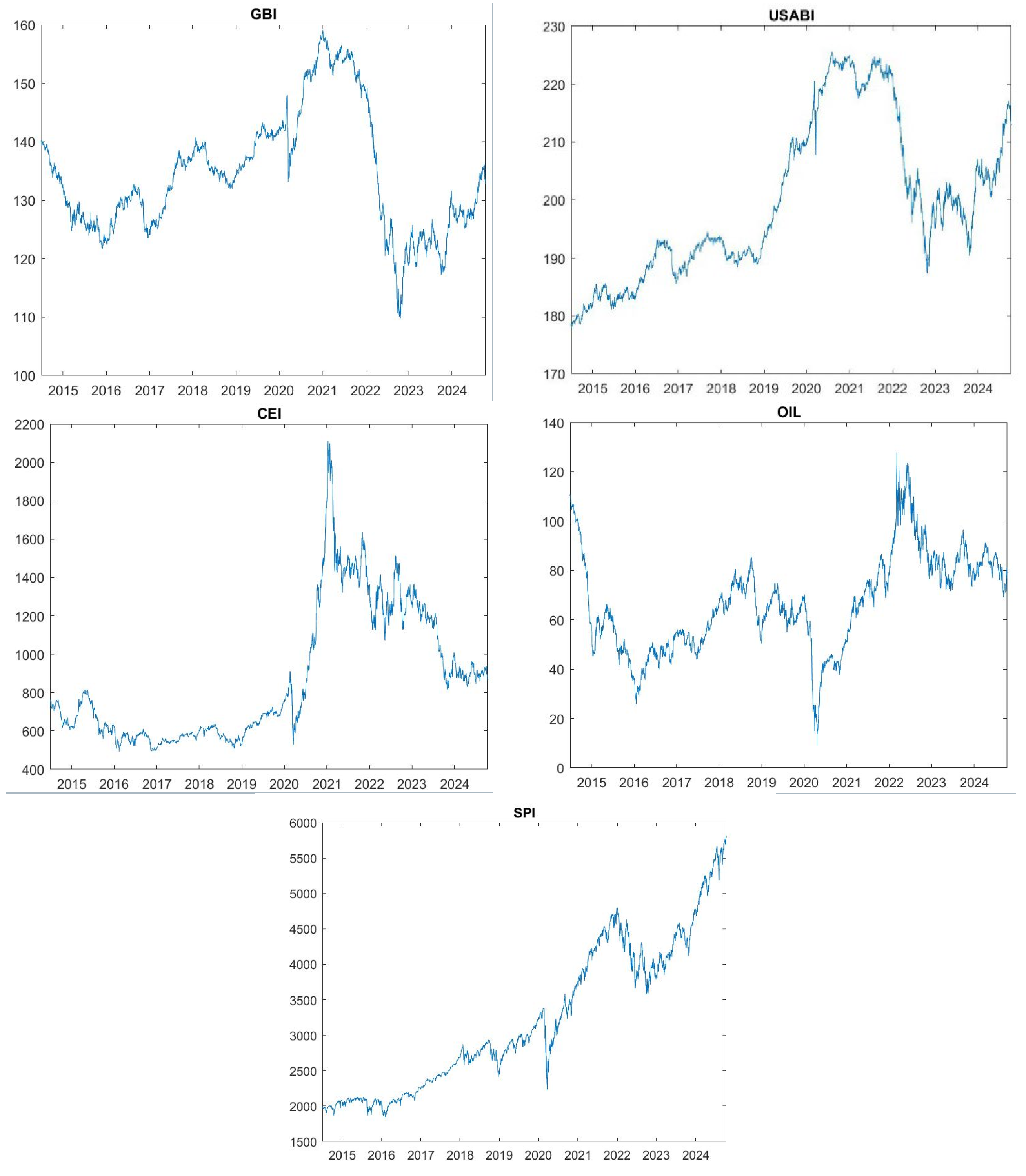
Figure 1 displays the time paths of the four considered variables. We observe that the green and conventional bond indices show similar evolution until 2017, after which the former was issued at a premium, while the latter dived due to excess liquidity. However, the overall evolution of the S&P clean energy index went through a sliding phase between 2014 and 2017, then entered a rising trend during the second part of the period. Daily returns are calculated as the logarithmic difference between observations at time t and t − 1, as ln (P_t) − ln (P_t−1). The description of the variables is summarized in

Table A1. Variable description table.

Description	Variable	Definition	Source
GBI	S&P Dow Jones Green Bond Index	Launched in July 2014, it is a multi-currency benchmark that includes bonds issued by multilateral, government, and corporate issuers (ICMA, 2017) and whose proceeds are used to finance environmentally related projects.	S&P Dow Jones Indices LLC
USABI	S&P US Aggregate Bond Index	Tracks the performance of the aggregate US domestic bond market.	S&P Dow Jones Indices LLC
SPI	The S&P 500 Index	Represents the dynamics of the stock market. It consists of the largest 500 companies in the US.	S&P Dow Jones Indices LLC
CEI	S&P Clean Energy Index	Represents companies that focus on clean energy-related business.	S&P Dow Jones Indices LLC
OIL	ICE Brent crude oil continuous contracts index	It is the most traded oil in recent years.	US Energy Information Administration (EIA).
VIX	Equity market uncertainty	Measures the market’s expectation of future volatility in financial markets.	The Chicago Board Options Exchange website
EPU	Economic Policy Uncertainty	Measured through newspaper coverage frequencies of economic policy-related discussions.	Economic Policy Uncertainty website

.

3.2. Cross-Quantilogram Approach

This paper measures the dependence structures across the full quantile range between green bonds and a set of financial markets through the cross-quantilogram (CQ) approach developed by Han et al. (2016). Applying this method requires the stationarity of the time series, which is validated by the unit root tests.

The CQ is particularly well-adapted to this analysis for three reasons. First, it is a non-parametric estimator built from quantile hit indicator processes, which means it does not require any distributional assumptions about the observed data. Second, despite the common presence of empirical features like heavy tails, skewness, and structural breaks in the data, the CQ remains valid. Third, unlike GARCH, VAR, or copula-based estimators that summarize dependence through moment-based statistics, the CQ measures conditional quantile dependence throughout the joint distribution. This feature allows the method to capture asymmetries and tail dependencies that often remain undetected by mean and variance-based approaches. Therefore, the CQ framework provides an empirically appropriate tool to identify how VIX and EPU reshape the dependence structure between green bonds and conventional bonds, equities, oil, and the clean energy index across distinct market regimes.

The quantile distribution of two variables is presented on the X-axis and the Y-axis through a heatmap. The cross-quantilogram considers large lags, which allows us to detect the direction, magnitude, and duration of the dependence between the variables (Uddin et al., 2019). Let $y_{1,t},y_{2,t},\dots ,y_{i,t}$, given that $y_{i,t}$ a stationary time series where $i=1,2, t=1,\dots ,T$. $F_i(\cdot )$ and $f_i(\cdot )$ are defined as the distribution and density functions of $y_{i,t}$, $i=1,2$, respectively. The cross-quantilogram measures dependence between two events, $\{y_{1,t}<q_{1,t}({\tau }_1\left)\right\}$ and $\{y_{2,t-k}<q_{2,t-k}({\tau }_2\left)\right\}$, for a random pair of τ2 = (τ₁, τ₂)′ and a positive integer k. Let $q_{i,t}\left({\tau }_i\right)$ be the quantiles, either ${\tau }_i$ conditional or unconditional, of $y_{i,t}$. The quantile hit or quantile exceedance process for $i=1,2,$ is presented as follows $\left\{1\right[y_{i,t}<q_{i,t}(\cdot )\left]\right\}$, where $1[.]$ denotes the indicator function. The conditional distribution function of the series $y_{it}$ given $x_{it}$ is denoted as $F_{y_i\mid x_i}(\cdot \mid x_{it})$, with its associated density function defined as $f_{y_i\mid x_i}(\cdot \mid x_{it})$. The corresponding conditional quantile function is represented by $q_{i,t}\left({\tau }_i\right)=inf\{v:F_i(v)\ge {\tau }_i\}$ where ${\tau }_i\in \left(\mathrm{0,1}\right)$ for $i=1,2$. The cross-quantilogram measures the cross-correlation of the quantile hit processes and is defined as:

$${\rho }_{\tau }\left(k\right)={\displaystyle \frac{E\left[{\psi }_{\tau 1}\left(y_{1,t}-q_{1,t}\left({\tau }_1\right)\right){\psi }_{{\tau }_2}\left(y_{2,t-k}-q_{2,t-k}\left({\tau }_2\right)\right)\right]}{\sqrt{E\left[{\psi }_{{\tau }_1}^2\left(y_{1,t}-q_{1,t}\left({\tau }_1\right)\right)\right]}\sqrt{E\left[{\psi }_{{\tau }_2}^2\left(y_{2,t-k}-q_{2,t-k}\left({\tau }_2\right)\right)\right]}}},$$

(1)

where $k$ indicates the number of lags in the series to time t ($k=0,\pm 1,\pm 2\dots )$ and ${\psi }_{r_i}(y_{i,t}-q_{i,t}({\tau }_i\left)\right)=1[y_{i,t}<q_{i,t}({\tau }_i\left)\right]-{\tau }_i$. The sample cross-quantilogram is defined as:

$${\widehat{\rho }}_{\tau }\left(k\right)={\displaystyle \frac{{\displaystyle {\sum }_{t=k+1}^T}{\psi }_{{\tau }_1}\left(y_{1,t}-{\widehat{q}}_{1,t}\left({\tau }_1\right)\right){\psi }_{{\tau }_2}\left(y_{2,t-k}-\widehat{q}2,t-k\left({\tau }_2\right)\right)}{\sqrt{{\displaystyle {\sum }_{t=k+1}^T}{\psi }_{{\tau }_1}^2\left(y_{1,t}-{\widehat{q}}_{1,t}\left({\tau }_1\right)\right)}\sqrt{{\displaystyle {\sum }_{t=k+1}^T}{\psi }_{{\tau }_2}^2\left(y_{2,t-k}-{\widehat{q}}_{2,t-k}\left({\tau }_2\right)\right)}}}.$$

(2)

Based on ${\hat{\rho }}_{\tau }\left(k\right)$, Han et al. (2016) propose a quantile version of the Ljung–Box-Pierce statistic with $H_0:{\rho }_{\tau }\left(1\right)=\cdots ={\rho }_{\tau }\left(p\right)=0$ for all $k\in 1,\dots ,p$ against the alternative $H_1:{\rho }_{\tau }\left(k\right)\ne 0$ for $k\in 1,\dots ,p$.

Using the cross-quantilogram, we can conduct related Portmanteau tests (Q-statistic), which can be used to test the directional predictability of events up to p lags. Statistical inference is based on the quantile version of the Ljung–Box test introduced by Han et al. (2016). This test evaluates directional predictability at specific lags and evaluates the lead–lag structure across quantile pairs. The Ljung–Box test takes the following form:

$${\widehat{Q}}_{\tau }\left(p\right)=T\left(T+2\right){\displaystyle \sum _{k=1}^p}{\displaystyle \frac{{\widehat{\rho }}^2\left(k\right)}{T-k}}.$$

(3)

3.3. Partial Cross-Quantilogram

As indicated earlier, the partial cross-quantilogram (PCQ) model is employed to control for the effect of macroeconomic factors on the cross-quantile dependence between green bonds and financial markets. The PCQ method is an extended version of the quantilogram, which controls for intermediate events between $t$ and $t-k$ and measures the relationship between two events $\{y_{1t}\le q_{1,t}({\tau }_1\left)\right\}$ and $\{y_{2t}\le q_{2,t}({\tau }_2\left)\right\}$. The control variables are represented by the vector ${\mathrm{z}}_t\equiv \left[{\psi }_{{\tau }_3}\right(y_{3t}-{q_{3,t}\left({\tau }_3\right)),\dots ,{\psi }_{{\tau }_l}(y_{lt}-q_{l,t}\left({\tau }_l\right)\left)\right]}^{\mathrm{\top }}$ where $l=3,\dots ,n$.

Han et al. (2016) define the correlation matrix of the hit processes and its inverse matrix as shown below:

$${R_{\overline{\tau }}=E[h_t\left(\overline{\tau }\right)h_t\left(\overline{\tau }{)}^{\mathrm{\top }}\right] \mathrm{a}\mathrm{n}\mathrm{d} P}_{\tau }=R_{\tau }^{-1},$$

(4)

where $h_t\left(\overline{\tau }\right)=\left[{\psi }_{{\tau }_1}\right(y_{1t}-q_{1,t}\left({\tau }_1\right)),\dots ,{\psi }_{{\tau }_l}(y_{lt}-{q_{l,t}\left({\tau }_l\right)\left)\right]}^{\mathrm{\top }}$ is a $l\times 1$ vector of the hit process.

The partial cross-quantilogram is defined as:

$${\rho }_{\overline{\tau }\mid \mathbf{z}}=-{\displaystyle \frac{p_{\overline{\tau },12}}{\sqrt{p_{\overline{\tau },11}{p}_{\overline{\tau },22}}}},$$

(5)

Given that ${\rho }_{\overline{\tau }\mid \mathbf{z}}$ is the cross-quantilogram dependence, which is conditional on the control variable z, it also has the following form:

$${\rho }_{\overline{\tau }\mid \mathbf{z}}=\delta \sqrt{{\displaystyle \frac{{\tau }_1\left(1-{\tau }_1\right)}{{\tau }_2\left(1-{\tau }_2\right)}},}$$

(6)

To ensure that the documented dependence structures are not driven by conditional heteroscedasticity, each return series is filtered through an AR(1)-GJR-GARCH (1,1) model with skewed-t innovations before the cross-quantilogram is reestimated. The AR(1) term captures short-run autocorrelation in the conditional mean, while the GJR-GARCH(1,1) models the conditional variance and captures the leverage effect. The skewed-t distribution models the heavy tails and asymmetry documented in the descriptive statistics. A single common specification is applied to all series, following the filtering procedure adopted by Han et al. (2016). The standardized residuals from these models are then used to re-estimate the cross-quantilogram across all quantile pairs.

4. Empirical Results and Discussion

4.1. Descriptive Statistics

Figure 1, illustrating the evolution of asset prices, shows the non-stationary patterns of the assets. Since its launch in 2014, the S&P Green Bond Index (GBI) has shown an upward trend aligned with the increasing commitment to sustainability through the policies of the Paris Agreement. The index showed resilience during the COVID-19 crisis due to the worldwide green recovery policies implemented by governments. The S&P Global Clean Energy Index (CEI) exhibits a boom-and-bust pattern. Since 2019, the CEI has maintained an upward trajectory aligned with the increasing investor interest in ESG investments. Reaching its highest level in 2021, the clean energy boom was particularly driven by policymakers, namely the election of Joe Biden in 2020 and his pro-climate agenda. On the other hand, the Brent Crude Oil index (OIL) has shown volatile patterns driven by geopolitical events and macroeconomic factors. The fuel market experienced downward pressure from excess supply in 2014–2016, major price reductions from COVID-19 lockdowns in 2020, and subsequent price growth after Russia invaded Ukraine in 2022. The S&P 500 Index (SPI) has experienced a strong increase despite the remarkable events throughout its history, including the 2008 financial crisis, the COVID-19 crisis, and the 2022 post-pandemic inflation. The U.S. Aggregate Bond Index (USABI) displays an upward trend that has risen gradually, as many interest rates have declined over the last two decades. The index displayed its most detrimental performance in recent times during 2022 because of increasing inflation and rising interest rates, which damaged bond market values.

The descriptive statistical analysis, reported in

Table 1. Descriptive statistics for the daily returns.

	GBI	USABI	OIL	CEI	SPI	VIX	EPU
Mean	1.30 × 10−5	0.0002	−0.001	3.02 × 10−6	0.0003	0.0007	0.002
Std. Dev.	0.0043	0.0020	0.0359	0.0135	0.0115	0.0825	0.7432
Skewness	−0.5981	−0.6634	−2.9856	−1.2053	−1.0628	0.9948	0.510
Kurtosis	9.1364	9.6822	93.8741	20.0733	26.4849	9.0261	4.7738
Jarque–Bera	2388.880	2836.940	506,955.9	33,988.98	18,172.90	2461.673	189.203
ADF	−34.9125 **	−36.5956 **	−39.3773 **	−47.3967 **	−35.4726 **	−40.0324 **	−59.3892 **

Notes: GBI: S&P Green Bond Index; USABI: US Aggregate Bond Index; OIL: Brent index; CEI: S&P Clean Energy Index; SPI: S&P 500 index, VIX: Implied volatility index, EPU: US Economic Policy Uncertainty. The data are daily from July 2014 to October 2024. Descriptive statistics are computed using the logarithmic differences between daily observations from time t − 1 to time t. ** Indicates significance at 5% level.

, of the daily returns of green bonds and the financial market indices, reveals several stylized features. First, the mean daily returns are very close to zero across all variables, which is consistent with the behavior typically observed in high-frequency financial data. Among the asset returns, OIL records a slightly negative mean, whereas GBI, USABI, CEI, SPI, and VIX exhibit small positive averages. EPU also shows a positive mean, but it stands out as the most volatile series in the sample, indicating pronounced fluctuations in policy uncertainty over the period under study. In contrast, the fixed-income variables, particularly GBI and USABI, display the lowest standard deviations, suggesting relatively stable return dynamics compared with equities, commodities, and uncertainty measures. This pattern is consistent with the notion that bond markets, and green bonds in particular, tend to exhibit lower short-term variability than riskier asset classes. The skewness coefficients further indicate that the distributions are not symmetric. GBI, USABI, OIL, CEI, and SPI are negatively skewed, implying that extreme negative returns occur more frequently than extreme positive returns. By contrast, VIX and EPU are positively skewed, reflecting occasional upward spikes in market volatility and policy uncertainty, especially during periods of heightened stress such as the COVID-19 pandemic and the Russia–Ukraine conflict. Kurtosis values are high across all series, most notably for OIL, CEI, and SPI, which confirms the presence of fat tails and excess kurtosis relative to the normal distribution. Skewness and excess kurtosis indicate the presence of non-normality in the series and suggest that extreme fluctuations occur more frequently than would be expected under a normal distribution. These characteristics motivate the use of an econometric approach that can capture both non-normal distributions and tail dependence. Finally, the Augmented Dickey–Fuller test statistics reject the null of a unit root for all series at the 5% significance level, indicating that the return series are stationary and suitable for further econometric analysis.

The pronounced volatility clustering and heavy tails documented in the descriptive statistics raise the possibility that part of the tail dependence identified above reflects synchronous volatility regimes rather than genuine directional predictability. To address this, each return series is filtered through an AR (1)-GJR-GARCH (1,1) model. The associated diagnostic tests are reported in Appendix A,

Table A3. AR(1)-GJR-GARCH (1,1) parameter estimates and filtering diagnostics.

Variables	ω	α	γ (Leverage)	β	LB(z2) p-Value	Resid. Kurtosis
GBI	0.0007 **	0.0248 *	0.0206 **	0.9600 ***	0.000	4.72
USABI	0.0006 ***	0.0705 ***	0.0030	0.9185 ***	0.338	4.11
OIL	0.1632 ***	0.0560 ***	0.0769 ***	0.8789 ***	0.869	5.40
SPI	0.0262 ***	0.0222	0.2792 ***	0.8226 ***	0.842	6.61
CEI	0.0294 ***	0.0433 ***	0.0819 ***	0.9052 ***	0.521	7.65

***, **, and * denote statistical significance at the 1%, 5%, and 10% levels, respectively.

. The leverage term is positive and statistically significant for the green bond, oil, equity, and clean energy series, confirming the presence of asymmetric volatility responses. The filtering effectively removes conditional heteroscedasticity: the Ljung–Box test on the squared standardized residuals is insignificant for the conventional bond, oil, equity, and clean energy series. The principal dependence structures are preserved: the positive tail dependence between green and conventional bonds remains the dominant relationship, and the directional patterns involving the equity, oil, and clean energy markets are unchanged in sign. Consistent with Han et al. (2016), the magnitude of the tail dependencies is attenuated once volatility dynamics are removed, indicating that a portion of the raw tail dependence was associated with common volatility regimes rather than genuine directional predictability. Overall, the dependence structures documented in this study are robust in sign and pattern to volatility filtering.

4.2. Cross-Quantile Correlations

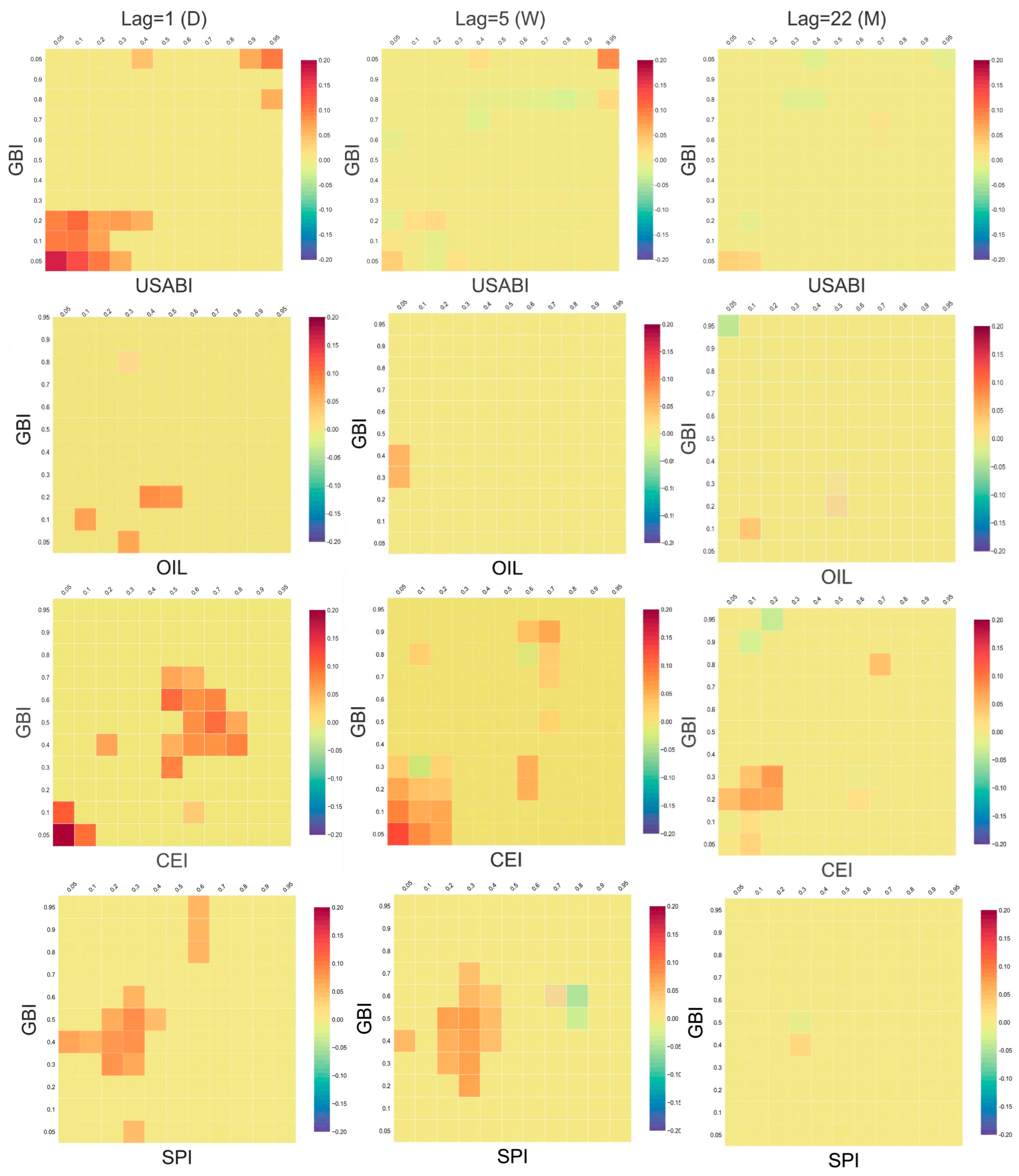
Cross-quantile correlations are employed to determine the symmetrical or asymmetrical nature of the relationship between green bonds and financial markets. Based on the tail and average dependencies, it can be shown whether green bonds are a safe haven or hedge against financial market fluctuations. Green bonds are a weak hedge when they are uncorrelated with other assets on average. They act as a weak safe haven if there is no dependence in lower quantiles and as a strong safe haven if negative dependence exists. A diversifier is an asset that is weakly positively correlated with another asset on average. Figure 2 presents the directional dependence from financial markets to the green bond market over different time frames (lags of 1, 5, and 22 days). The results are illustrated through heatmaps where the color scale indicates dark blue for negative dependence, yellow for no correlation, and dark red for highly positive dependence. The x-axis displays the quantiles of green bonds, and the y-axis displays the quantiles of the other assets.

According to the Ljung–Box test from Equation (3), a non-significant correlation is considered zero. The impact of conventional bonds (USABI) on green bonds (GBI) is depicted in the first heatmap (lag 1) to identify the presence of tail dependence. This indicates that USABI and GBI experience simultaneous surges and declines during different market events. This is consistent with the findings of Reboredo (2018), who shows that green and conventional bonds strongly co-move. Conversely, there is a very weak positive correlation with no evidence of tail dependence between oil and green bonds. The absence of dependence on average suggests that green bonds are used for diversification by investors in the oil market, which is in contrast with Reboredo (2018), who provides evidence of weak co-movement and tail dependence between green bond and energy commodity markets under regular market conditions. This may be due to the fact that the previous study examined a broader global energy market index, while the current research focused on the US oil market. Regarding the stock market, there is no tail dependence, which makes green bonds a good diversifier for investors in this market. Similarly, Reboredo (2018) finds that the green bond market weakly co-moves with the stock market as represented by the MSCI World Index (MSCI).

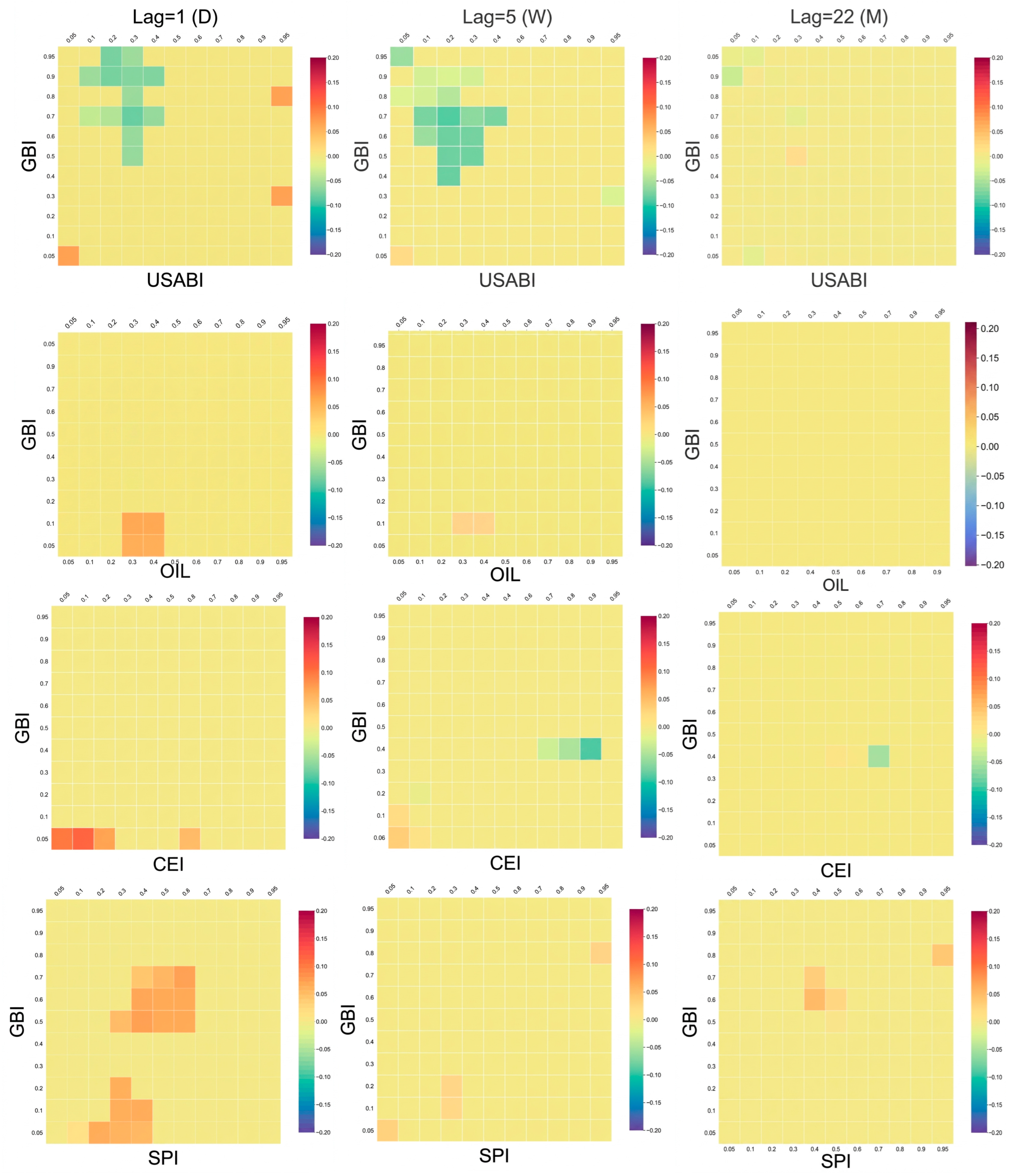
Furthermore, there is weak dependence in the lower quantiles between GBI and clean energy stocks (CEI), while there is a positive dependence on average. Thus, this indicates that green bonds serve as a weak diversifier for clean energy investors. As we move to longer lags, the influence of financial markets on green bonds deteriorates over time; it persists over one week and vanishes over one month. This suggests that over one week, the previously mentioned markets do not influence green bonds, proving that investors in these financial markets react similarly to information over short timeframes. Figure 3 presents the results of reverse bidirectionality, examining the influence of green bonds on financial markets. There is a negative asymmetric spillover from the green bond market to the fixed-income market, suggesting that green bonds exert a negative influence on conventional bonds when they have positive returns. Investors prefer green bonds over regular bonds, highlighting that they adopt opposite strategies in the two markets. The intensity of predictability persists after one week (lag 5), highlighting investors’ differing reactions to new information in both markets. We observe a symmetric positive spillover from GBI to SPI within the middle quantiles in the stock market, indicating a symmetric relationship under regular market conditions. This implies that green bonds can serve as a diversifier in the stock market. In the energy market, the negative dependence between green bonds and oil and clean energy stocks is primarily observed under normal market conditions. This indicates that the relationship between these assets is most pronounced during typical market fluctuations. These findings underscore the role of green bonds in portfolio diversification, particularly within stable market environments. The empirical results are summarized in

Table A2. Summary of cross-quantilogram results.

Correlations from Financial Markets to the Green Bond Market
Variables	Results	Interpretations
USABI-GBI	USABI has an impact on GBI.	Green and conventional bonds undergo booms and busts simultaneously.
OIL-GBI	No particular correlations.	Green bonds are considered diversifiers for investors in the oil market.
SPI-GBI	No tail dependence, with small dependence in the rest of the quantiles.	Green bonds act as a diversifier in the stock market.
CEI-GBI	Little dependence in lower quantiles and average positive dependence.	Used for diversification in the clean energy market.
The influence of financial markets on green bonds persists over one week (lag 5) and vanishes over one month (lag 22). The dependence structures deteriorate over time: Over one week, the above-mentioned markets no longer affect green bonds, proving that investors in these financial markets react similarly to information in a short period.
Correlation from the Green Bond Market to Financial Markets
Variables	Results	Interpretations
GBI-USABI	Negative correlation among the upper and lower quantiles.	When green bonds have positive returns, they have a negative influence on conventional bonds, which makes investors tend to buy green bonds rather than regular bonds.
GBI-SPI	Positive spillover when they are in the middle.	There are homogeneous dependence structures between these assets, which implies a symmetric spillover relationship in regular market conditions, making green bonds a good diversifier in the stock market.
GBI-OIL	GBI has little influence on OIL.	Investors in the green bond market can diversify their portfolios by investing in OIL.
GBI-CEI	Small correlation	Investors in the green bond market can diversify their portfolios by investing in CEI.
The intensity of predictability holds out after one week (lag 5), proving the different behaviors of investors towards new information in both markets. The relationship between green bonds and conventional bonds is asymmetric. The relationship between green bonds, stock, oil, and clean energy markets is symmetric.

.

4.3. The Effect of Uncertainties on the Dependence Structures

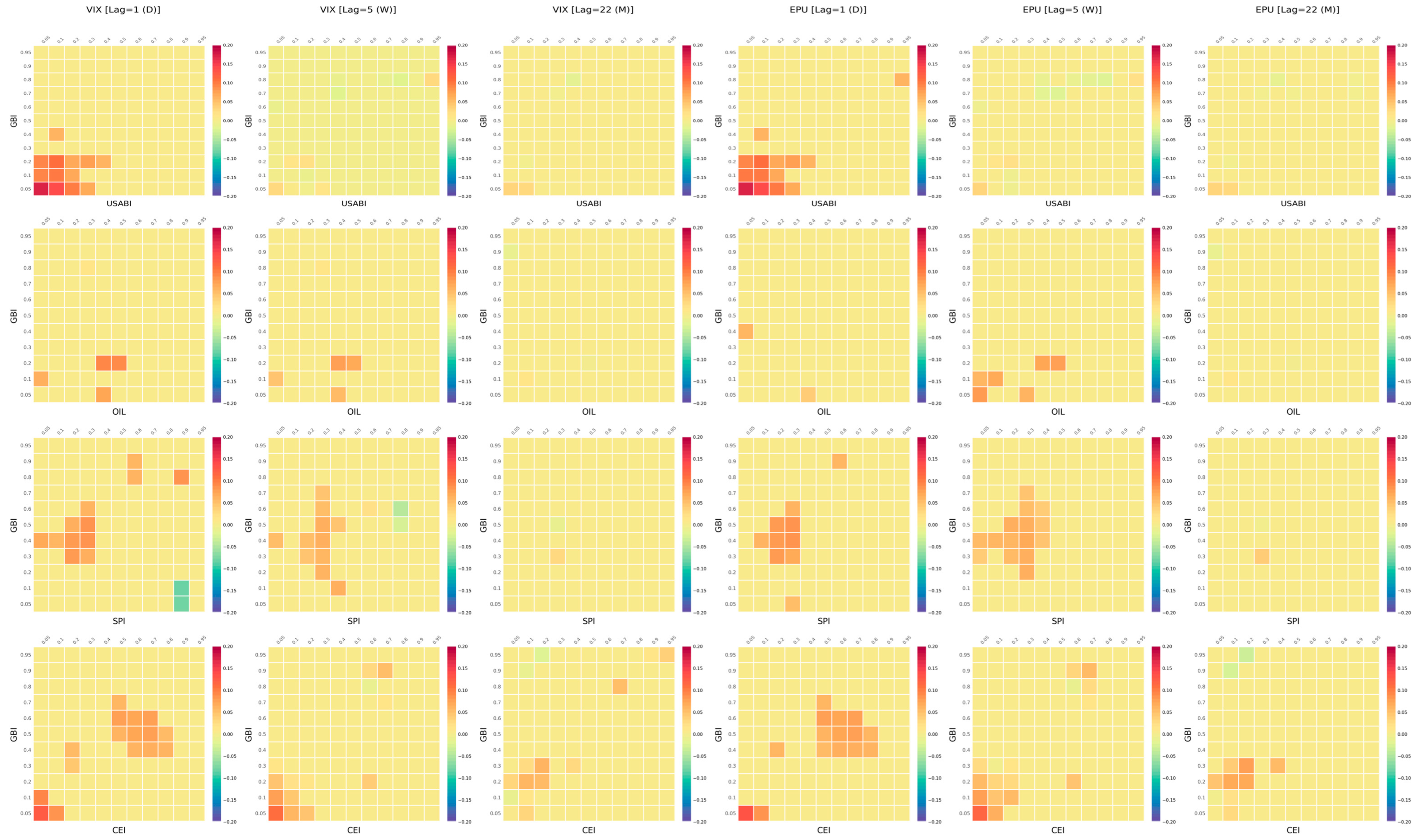
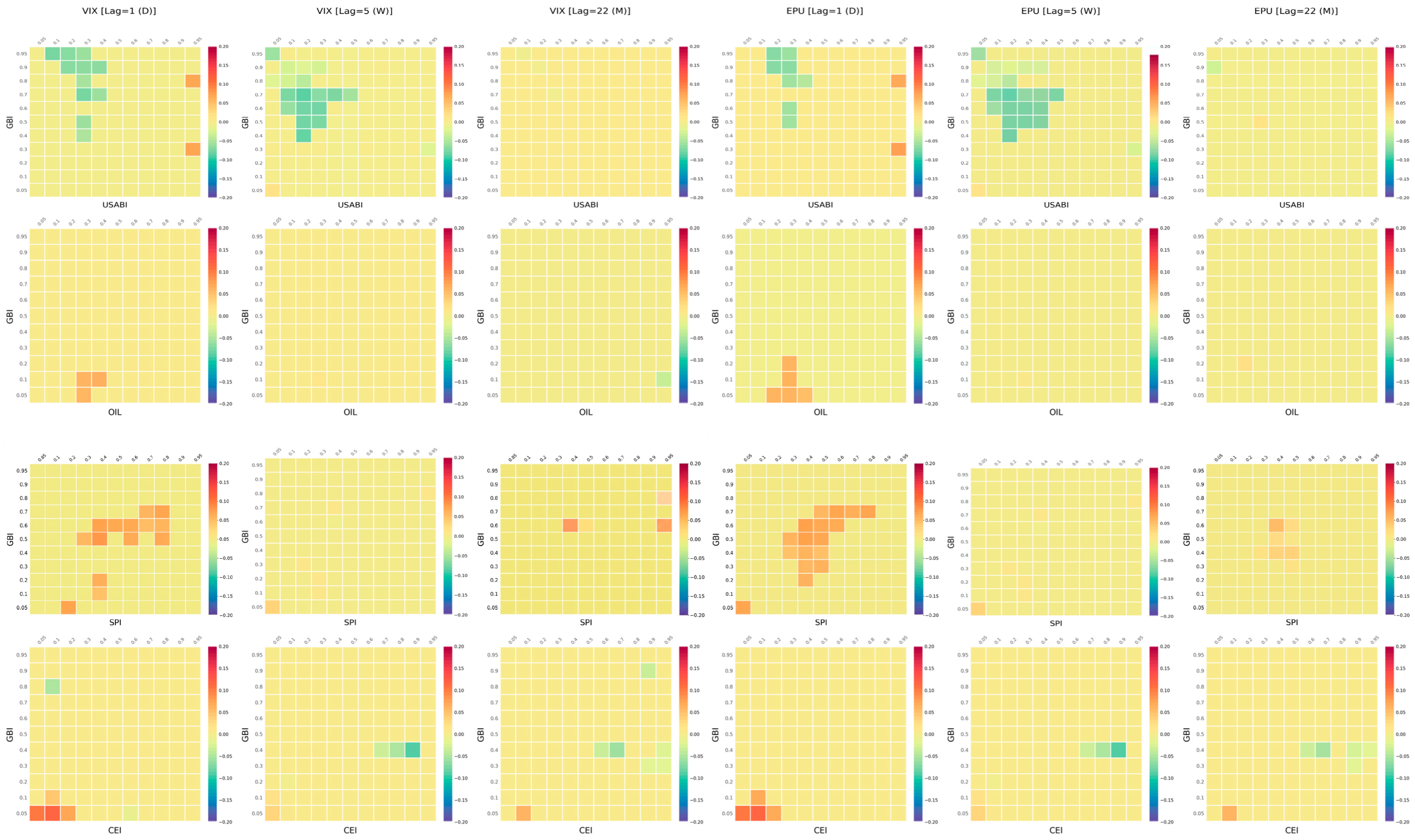
To assess whether VIX and EPU drive the dependence structures previously documented, the analysis is extended through the partial cross-quantilogram (PCQ). Figure 4 and Figure 5 present the results of the PCQ after introducing the uncertainty factors as conditioning variables. The results reveal that the cross-quantile correlations remain unchanged, as only marginal differences exist compared to the full cross-quantilogram results (Figure 2 and Figure 3). This indicates that neither EPU nor VIX shapes the dependence structures of green bonds and the studied financial assets. Therefore, this suggests that market-specific drivers may be the primary influence on the relationship between green bonds and financial assets, rather than macroeconomic factors. Several factors could be considered in this regard, namely liquidity risk, as when the market is less liquid, prices respond more slowly to new information, which could affect the dynamic co-movement structure between green bonds and financial assets under study (Febi et al., 2018). Nevertheless, liquidity conditions are considerably shaped by the regulatory framework governing the green bond market, given that green taxonomies and ESG disclosure obligations determine the depth and composition of investor participation. Reflecting the degree of ambiguity surrounding environmental legislation and international climate commitments, climate policy uncertainty (CPU) is more directly aligned with the green bond market, as it may modify the hedging properties of green bonds during regulatory changes.

To formally assess whether conditioning on VIX and EPU alters the dependence structure, we complement the visual comparison of the cross-quantilogram and partial cross-quantilogram with quantitative evidence. For each asset pair, we compute the difference between the unconditional and partial cross-quantilogram across the full quantile grid, and we test the null hypothesis that the two are equal using a stationary bootstrap that jointly resamples the series to preserve their cross-dependence. The test yields both cell-wise significance and a joint statistic summarizing equality across the entire grid, and the difference measures are reported in

Table 2. Difference between the unconditional (CQ) and partial (PCQ) cross-quantilograms conditioning on VIX and EPU.

Conditioning	Asset Pair	Mean Abs. Difference	Max Abs. Difference	Joint Test (p-Value)
VIX	USABI → GBI	0.0024	0.0093	0.020
VIX	OIL → GBI	0.0035	0.0114	0.010
VIX	SPI → GBI	0.0066	0.0251	0.000
VIX	CEI → GBI	0.0042	0.0155	0.007
EPU	USABI → GBI	0.0019	0.0069	0.057
EPU	OIL → GBI	0.0008	0.0033	0.277
EPU	SPI → GBI	0.0019	0.0066	0.037
EPU	CEI → GBI	0.0019	0.0064	0.064

.

Table 2 reports the difference measures between the CO and PCQ for each asset pair, obtained after conditioning on VIX and EPU, respectively. The evidence indicates that conditioning on aggregate uncertainty leaves the dependence structure substantively intact. Across all asset pairs, the average absolute difference between the two estimates remains below 0.01, and the maximum difference recorded at any single quantile cell does not exceed 0.025, a magnitude that is economically negligible when set against the unconditional CQ values, which reach 0.175 for the green bond–conventional bond relationship. Conditioning on EPU produces the smaller adjustments of the two, with average absolute differences between 0.0008 and 0.0019 and no change to the dependence structure for the majority of asset pairs. Conditioning on VIX yields marginally negligible differences, with the most pronounced adjustment observed for the equity relationship. Taken together, these formal difference measures corroborate the conclusion previously drawn from the visual comparison of the heatmaps: neither VIX nor EPU meaningfully shapes the cross-quantile dependence between green bonds and the financial assets under study, reinforcing the interpretation that the documented dependence structures are governed by factors specific to the green bond market rather than by aggregate macroeconomic uncertainty.

5. Conclusions

ESG-aligned investments attract investors who seek to integrate ethical considerations into their portfolio strategies. The intense demand for sustainable investment has led to the emergence of green bonds, a powerful financial tool that integrates environmental goals with investment approaches. The evaluation of their diversification potential requires a thorough understanding of their relationships with broader financial markets. This research investigates the nexus between green bonds and major financial assets, namely conventional bonds, oil, equities, and clean energy, under different economic scenarios, and evaluates whether EPU and VIX influence these dependencies. The results reveal that green and conventional bonds exhibit significant tail dependence, indicating synchronized booms and busts. Thus, green bonds can serve as a diversifier for investors in equities, oil, and clean energy markets during periods of turmoil. The strength of the connectedness between all assets is most pronounced in the short term and tends to weaken over time, which is crucial for investors with different time horizons. After including EPU and VIX, the dependence structures persist with marginal differences, suggesting that neither of these uncertainty measures has a meaningful impact on the co-movement structures. This may be related to the distinct characteristics of investor sentiment within the green bond market and to other factors, such as sustainability-specific uncertainty and regulatory changes, that may play a more significant role in shaping dependence structures. Accordingly, an extension of the present analysis could employ the CPU index, which captures the thematic dimensions of uncertainty that are most likely to shape green bond linkages with other financial markets. As the green finance market continues to expand, a deep understanding of these dynamics is increasingly important for building responsible and ethical investment strategies.

References

1. Bachelet, M. J., Becchetti, L., & Manfredonia, S. (2019). The green bonds premium puzzle: The role of issuer characteristics and third-party verification. Sustainability, 11(4), 1098. [Google Scholar] [CrossRef] [Scilit]
2. Baker, M., Bergstresser, D., Serafeim, G., & Wurgler, J. (2018). Available online: https://www.nber.org/papers/w25194 (accessed on 12 December 2025).
3. Belguith, R. (2025). Dynamics of green and conventional bonds: Hedging effectiveness and sustainability implication. International Journal of Financial Studies, 13(2), 106. [Google Scholar] [CrossRef] [Scilit]
4. Broadstock, D. C., & Cheng, L. T. W. (2019). Time-varying relation between black and green bond price benchmarks: Macroeconomic determinants for the first decade. Finance Research Letters, 29, 17–22. [Google Scholar] [CrossRef] [Scilit]
5. Climate Bonds Initiative. (2025). Sustainable debt global state of the market 2024. Available online: https://www.climatebonds.net/data-insights/publications/global-state-market-2024 (accessed on 12 November 2025).
6. Diebold, F. X., & Yilmaz, K. (2012). Better to give than to receive: Predictive directional measurement of volatility spillovers. International Journal of Forecasting, 28(1), 57–66. [Google Scholar] [CrossRef] [Scilit]
7. Febi, W., Schäfer, D., Stephan, A., & Sun, C. (2018). The impact of liquidity risk on the yield spread of green bonds. Finance Research Letters, 27, 53–59. [Google Scholar] [CrossRef] [Scilit]
8. Fernandes, L. H. S., Silva, J. W. L., de Araujo, F. H. A., & Tabak, B. M. (2023). Multifractal cross-correlations between green bonds and financial assets. Finance Research Letters, 53, 103603. [Google Scholar] [CrossRef] [Scilit]
9. Flaherty, M., Gevorkyan, A., Radpour, S., & Semmler, W. (2017). Financing climate policies through climate bonds—A three stage model and empirics. Research in International Business and Finance, 42, 468–479. [Google Scholar] [CrossRef] [Scilit]
10. Flammer, C. (2021). Corporate green bonds. Journal of Financial Economics, 142(2), 499–516. [Google Scholar] [CrossRef] [Scilit]
11. Gianfrate, G., & Peri, M. (2019). The green advantage: Exploring the convenience of issuing green bonds. Journal of Cleaner Production, 219, 127–135. [Google Scholar] [CrossRef] [Scilit]
12. Han, H., Linton, O., Oka, T., & Whang, Y. J. (2016). The cross-quantilogram: Measuring quantile dependence and testing directional predictability between time series. Journal of Econometrics, 193(1), 251–270. [Google Scholar] [CrossRef] [Scilit]
13. ICMA. (2017). Summary of green fixed income indices providers. ICMA. [Google Scholar]
14. Karpf, A., & Mandel, A. (2018). The changing value of the “green” label on the US municipal bond market. Nature Climate Change, 8(2), 161–165. [Google Scholar] [CrossRef] [Scilit]
15. Liu, N., Liu, C., Da, B., Zhang, T., & Guan, F. (2021). Dependence and risk spillovers between green bonds and clean energy markets. Journal of Cleaner Production, 279, 123595. [Google Scholar] [CrossRef] [Scilit]
16. Naeem, M. A., Bouri, E., Costa, M. D., Naifar, N., & Shahzad, S. J. H. (2021). Energy markets and green bonds: A tail dependence analysis with time-varying optimal copulas and portfolio implications. Resources Policy, 74, 102418. [Google Scholar] [CrossRef] [Scilit]
17. Park, D., Park, J., & Ryu, D. (2020). Volatility spillovers between equity and green bond markets. Sustainability, 12(9), 3722. [Google Scholar] [CrossRef] [Scilit]
18. Pham, L. (2016). Is it risky to go green? A volatility analysis of the green bond market. Journal of Sustainable Finance and Investment, 6(4), 263–291. [Google Scholar] [CrossRef] [Scilit]
19. Pham, L., & Nguyen, C. P. (2022). How do stock, oil, and Economic Policy Uncertainty influence the green bond market? Finance Research Letters, 45, 102128. [Google Scholar] [CrossRef] [Scilit]
20. Reboredo, J. C. (2018). Green bond and financial markets: Co-movement, diversification and price spillover effects. Energy Economics, 74, 38–50. [Google Scholar] [CrossRef] [Scilit]
21. Reboredo, J. C., & Ugolini, A. (2020). Price connectedness between green bond and financial markets. Economic Modelling, 88, 25–38. [Google Scholar] [CrossRef] [Scilit]
22. Reboredo, J. C., Ugolini, A., & Aiube, F. A. L. (2020). Network connectedness of green bonds and asset classes. Energy Economics, 86, 104629. [Google Scholar] [CrossRef] [Scilit]
23. Siddique, M. A., Nobanee, H., Hasan, M. B., Uddin, G. S., & Nahiduzzaman, M. (2024). Is investing in green assets costlier? Green vs. non-green financial assets. International Review of Economics and Finance, 92, 1460–1481. [Google Scholar] [CrossRef] [Scilit]
24. Tang, D. Y., & Zhang, Y. (2020). Do shareholders benefit from green bonds? Journal of Corporate Finance, 61, 101427. [Google Scholar] [CrossRef] [Scilit]
25. Uddin, G. S., Rahman, M. L., Hedström, A., & Ahmed, A. (2019). Cross-quantilogram-based correlation and dependence between renewable energy stock and other asset classes. Energy Economics, 80, 743–759. [Google Scholar] [CrossRef] [Scilit]
26. Wei, P., Yuan, K., Ren, X., Yan, C., & Lu, Z. (2023). Time-varying spillover networks of green bond and related financial markets. International Review of Economics and Finance, 88, 298–317. [Google Scholar] [CrossRef] [Scilit]
27. Zerbib, O. D. (2019). The effect of pro-environmental preferences on bond prices: Evidence from green bonds. Journal of Banking and Finance, 98, 39–60. [Google Scholar] [CrossRef] [Scilit]
28. Zheng, J., Jiang, Y., Cui, Y., & Shen, Y. (2023). Green bond issuance and corporate ESG performance: Steps toward green and low-carbon development. Research in International Business and Finance, 66, 102007. [Google Scholar] [CrossRef] [Scilit]
Figure 1. Asset price dynamics.
Ijfs 14 00219 g001
Figure 2. Cross-quantilogram correlation heatmaps between green bond returns and asset markets: Asset markets return to green bonds.3
Ijfs 14 00219 g002
Figure 3. Cross-quantilogram correlation heatmaps: the spillover from green bond returns to asset markets.
Ijfs 14 00219 g003
Figure 4. Partial cross-quantilogram correlations between green bonds and financial asset returns after controlling for uncertainties.
Ijfs 14 00219 g004
Figure 5. Partial cross-quantilogram correlations from green bond returns to asset markets after controlling for uncertainties.
Ijfs 14 00219 g005