A Framework for Gold Price Prediction Combining Classical and Intelligent Methods with Financial, Economic, and Sentiment Data Fusion

Abstract

Accurate gold price forecasting is essential for informed financial decision-making, as gold is sensitive to economic, political, and social factors. This study presents a hybrid framework for multivariate gold price prediction that integrates classical econometric modelling, traditional machine learning, modern deep learning methods, and their combinations. The framework incorporates financial, macroeconomic, and sentiment indicators, allowing it to capture complex temporal patterns and cross-variable relationships over time. Empirical validation on an eleven-year dataset (2014–2024) demonstrates the framework effectiveness across diverse market conditions. Results show that advanced supervised techniques outperform traditional econometric models under dynamic market environment. Key advantages of the framework include its ability to handle multiple data types, apply a structured variable selection process, employ diverse model families, and support model hybridisation and meta-modelling, providing practical guidance for investors, institutions, and policymakers.

1. Introduction

Gold remains a strategic asset in global finance, recognized for its role as both a store of value and a hedge against inflation, currency risk, and geopolitical uncertainty (Reboredo, 2013). It is traded in various forms, including physical bullion, ETFs, and derivatives. Among these, gold futures stand out for their liquidity, standardization, and responsiveness to economic conditions, making them well suited for predictive modelling. Gold futures contracts (GC = F), commonly used as hedging tools and safe-haven assets, have gained prominence for their ability to mitigate price volatility (Fang et al., 2018). As they represent a growing share of global commodity trading (CME Group, 2025), interest in advanced forecasting methods, especially deep learning (DL), has increased, driven by the need to capture complex market dynamics and improve predictive accuracy.

The heightened volatility in gold prices has raised concerns about financial stability among policymakers, economists, and investors. Empirical studies confirm that gold price movements are closely linked to macroeconomic uncertainty, including inflation expectations, exchange rate fluctuations, and central bank interest rate policies (Beckmann et al., 2019). In addition to traditional macroeconomic indicators, sentiment has emerged as a critical factor influencing financial markets. In machine learning (ML), sentiment typically refers to the computational classification of opinions in text as positive, negative, or neutral (Liu, 2012). Social sentiment, more broadly, reflects the collective emotional or attitudinal responses of a population to events or topics, often extracted from news sources and social media (Cortis & Davis, 2021). Advances in information technologies now enable real-time monitoring of such sentiment, significantly increasing the volume and diversity of available data. Understanding these influencing factors is essential for effective risk management, informed monetary policy, and the promotion of stable and transparent financial systems.

Recent trends indicate increasing global demand for gold (WGC, 2025), accompanied by shifts in trade patterns and more assertive investment strategies aimed at managing financial uncertainty. Gold futures trading volumes are rising steadily, particularly in both developed and emerging markets where inflation and geopolitical tensions shape investor behaviour (Raza et al., 2018). In response, financial institutions are diversifying their offerings through leveraged gold instruments and digital trading platforms, aiming to attract risk-sensitive investors and maintain competitiveness (Gold Trading Platforms, 2024).

Despite its growing importance, gold price forecasting still lacks a unified framework that incorporates the diverse set of influencing factors. Predicting gold movements remains a complex problem for two main reasons:

• First, gold prices are shaped by a broad and interconnected set of factors, financial, macroeconomic, and geopolitical, which interact in dynamic and unstable environment. Market indicators such as equity indices, bond yields, and commodity prices reflect investor attitudes, while geopolitical shocks, captured by risk indices, can trigger sudden shifts in market state (Baur & Smales, 2020). The nonlinear nature of these relationships complicates efforts to represent gold price behaviour within a single modelling structure.
• Second, the increasing availability of high frequency and sentiment-related data requires more sophisticated forecasting techniques. Traditional models such as ARIMA (Adebiyi et al., 2014) and GARCH (Kristjanpoller & Minutolo, 2015) offer foundational insights, but often struggle to capture complex, nonlinear dynamics (Qiu et al., 2024). Recent advances in information technology now permit real-time monitoring of social sentiment and market behaviour, expanding the scope and granularity of data available for forecasting. Consequently, DL techniques are adopted (Fischer & Krauss, 2018) for their ability to model sequential dependencies and uncover hidden patterns in high-dimensional data.

These challenges motivate the development of an integrated forecasting framework that brings together financial indicators, macroeconomic variables, and sentiment-based measures to improve gold price prediction. According to the framework, the process begins with collecting a dataset that includes key economic indicators, commodity prices, and sentiment indices. Next, after a preprocessing, a representative subset of predictive variables is selected using a combination of statistical analyses and model-based techniques. Finally, a range of forecasting models, from classical econometric approaches to modern DL architectures, is developed and evaluated across different market conditions.

The contributions of this study are as follows. The proposed forecasting framework integrates multi-type inputs, capturing a broader range of factors that influence gold price dynamics. A structured process for selection of appropriate independent variables is implemented, combining a variety of econometric and ML methods to ensure the relevance of inputs. The framework employs a diverse set of prediction methods, including classical econometric techniques, ML algorithms, DL architectures, and their hybrid forms, enabling a comprehensive model performance comparison. It also supports meta-modelling, allowing flexible model combinations to improve forecast accuracy and adaptability. Finally, by embedding explainable techniques, the framework offers transparency even in case of complex models and translates empirical results into actionable recommendations for stakeholders, operating in volatile market environments.

The remainder of the paper is structured as follows. Section 2 surveys recent work on gold-price prediction, with particular attention to the economic, financial, and sentiment-driven factors that influence price dynamics. Section 3 sets out the methodological framework, explaining the data sources, independent-variable selection procedure, and forecasting techniques. Section 4 empirically evaluates the effectiveness of the proposed framework by addressing the problem of gold futures price prediction, using an eleven-year multivariate dataset composed of diverse input variables. Section 5 concludes by summarising the main findings, acknowledging the study’s limitations, and outlining future research directions.

2. Related Work

In this section, we review recent studies on gold price forecasting with emphasis on both the types of data used and the modelling techniques applied. The analysis compares key aspects such as target variables, input features, modelling approaches, and evaluation metrics, highlighting current trends and best practices that support the development of data-driven and interpretable gold price forecasting frameworks.

Hajek and Novotny (2022) presented an interpretable fuzzy rule-based framework combining financial variables with news sentiment for short-term gold price forecasting. Their findings highlight the relevance of sentiment for one-day-ahead predictions, while traditional financial indicators remain more effective over longer horizons. The model balances predictive accuracy with transparency through rule-based insights.

Liang et al. (2022) proposed a hybrid framework (ICEEMDAN-LSTM-CNN-CBAM) that integrates signal decomposition and DL. The model uses Improved Complete Ensemble Empirical Mode Decomposition with Adaptive Noise (ICEEMDAN) to extract time series components, which are then processed by a combined Long Short-Term Memory (LSTM)–Convolutional Neural Network (CNN) architecture with an attention mechanism (Convolutional Block Attention Module (CBAM)). Their results show that this approach significantly outperforms conventional and hybrid baselines, as confirmed by the Model Confidence Set (MCS) test.

Mamoudan et al. (2023) developed a hybrid DL framework combining CNN and Bidirectional Gated Recurrent Unit (BiGRU) networks, with hyper-parameters optimized via metaheuristic algorithms such as the Grey Wolf Optimizer (GWO), Artificial Bee Colony Algorithm (ABC), Earthworm Optimization Algorithm (EWA), BAT algorithm (BAT), and Firefly Algorithm (FA). Trained on 112 technical indicator-based features from 10 months of gold market data, the model demonstrated the effectiveness of integrating neural networks with metaheuristics for classification and prediction in highly volatile commodity markets.

Stanković et al. (2023) introduced a univariate forecasting model based on a Bidirectional LSTM (BiLSTM) network, enhanced by an Improved Teaching–Learning Based Optimization (ITLB) algorithm and Variational Mode Decomposition (VMD) for signal preprocessing. Evaluated on daily gold prices from 2020 to 2022, the VMD-BiLSTM-ITLB model outperformed alternative metaheuristic-based methods, showing robustness and forecasting accuracy in multi-step forecasting.

Amini and Kalantari (2024) designed a hybrid DL framework combining a CNN and BiLSTM for gold price prediction. Their model leverages the CNN for spatial feature extraction and BiLSTM for temporal modelling, effectively capturing nonlinear dynamics in gold price behaviour.

Pokou et al. (2024) created a hybrid framework that combines ARIMA processes and ML models to enhance stock market forecasting. By incorporating temporal dependencies and feature attention, the model addresses limitations of traditional time series methods. Using daily data from 2012 to 2022, it outperformed standard LSTM, GRU, and other ML baselines in predictive accuracy.

Qiu et al. (2024) built a two-stage hybrid DL framework that first applies VMD for time series clustering, followed by a residual correction step using backpropagation (BP), LSTM, and CNN models. Tested on gold futures data from four major markets, the model outperforms single-model approaches in prediction accuracy.

Tashakkori et al. (2024) proposed a new model based on Multi-layer Perceptron (MLP) neural networks for forecasting gold prices using gold trading data. Unlike hybrid DL approaches, the study focuses on assessing the standalone performance of an optimized MLP architecture using historical gold prices, specifically the Open, High, Low, Close prices, and trading Volume (OHLCV) as input features. The results show that the model achieves competitive accuracy, offering a lightweight and efficient option for financial time series prediction.

In their study, Zangana and Obeyd (2024) created a DL-based framework for gold price forecasting using historical time series data. The authors employ LSTM and BiLSTM models to capture temporal dependencies and improve prediction accuracy. The model inputs include key economic indicators such as crude oil prices, exchange rates, inflation, and interest rates. SHapley Additive exPlanations (SHAP) analysis revealed that crude oil and USD/EUR exchange rates were key contributors to prediction performance.

Table 1. Summary of recent studies on gold price forecasting.

Reference	Research Objective	Dataset Characteristics	Prediction Methods	Model Evaluation
(Hajek & Novotny, 2022)	Framework for gold price prediction using different indicators and news sentiment	Gold futures, financial indicators, news sentiment (2007–2017)	FURIA with evolutionary tuning	Accuracy, AUC, interpretability via IF–THEN fuzzy rules
(Liang et al., 2022)	Hybrid DL-based prediction method	Gold futures and spot prices (2010–2020)	ICEEMDAN + LSTM + CNN + CBAM	MAE 1, MSE 2, RMSE 3, MAPE 4, SMAPE 5 in MCS test
(Mamoudan et al., 2023)	Hybrid DL-based framework using trading signals from technical indicators	112 features from MACD, Ichimoku, MA indicators (10 months of 2020)	CNN + BiGRU, optimized by GWO, ABC, EWA, BAT, and FA	Accuracy, Precision, Recall, F1, ROC-AUC
(Stanković et al., 2023)	Hybrid DL-based method with trend extraction and hyper-parameter optimization procedure	Gold prices (2020–2022)	VMD + BiLSTM + ITLB	MAE, MSE, RMSE, R2 6
(Amini & Kalantari, 2024)	Hybrid DL-based method with parameter tuning	Gold prices (1978–2021)	CNN + BiLSTM	MSE, RMSE, MAE, R2
(Pokou et al., 2024)	Hybrid ARIMA+ML methods	Gold prices (2016–2023, three periods)	ARIMA + ML combinations	RMSE, MAPE, NSE 7
(Qiu et al., 2024)	DL framework with features fusion and residual correction	Four gold futures series (2004–2022)	VMD + BP + CNN + LSTM	MSE, MAE, RMSE, R2, MAPE
(Tashakkori et al., 2024)	MLP-based model using gold trading features	Gold trading indicators OHLCV (2012–2022)	MLP	Loss rate
(Zangana & Obeyd, 2024)	Two LSTM variants with explainability	Gold prices and macroeconomic data (oil, USD/EUR, inflation, interest)	LSTM, BiLSTM, SHAP	MAE, RMSE, R2

¹ MAE—Mean Absolute Error, ² MSE—Mean Squared Error, ³ RMSE—Root Mean Squared Error, ⁴ MAPE—Mean Absolute Percentage Error, ⁵ sMAPE—symmetric Mean Absolute Percentage Error, ⁶ R²—Coefficient of Determination, ⁷ NSE—Nash–Sutcliffe Efficiency.

summarises recent models for gold price prediction, outlining modelling approaches, data sources, and variables used. These studies can be grouped based on several criteria, including research objectives, prediction methods, dataset characteristics, target variables, input types, modelling techniques, evaluation metrics, and overall predictive performance.

Based on the proposed methodologies, Hajek and Novotny, Mamoudan et al., and Qiu et al. introduced new multi-stage or hybrid forecasting frameworks aimed at improving predictive performance through techniques such as feature fusion, metaheuristics, or residual correction (Hajek & Novotny, 2022; Mamoudan et al., 2023; Qiu et al., 2024). In contrast, the rest of the studies presented new predictive methods, including hybrid DL architectures with automated parameter tuning (Liang et al., 2022; Stanković et al., 2023; Amini & Kalantari, 2024; Zangana & Obeyd, 2024), enhanced ARIMA (Pokou et al., 2024), and MLP-based (Tashakkori et al., 2024) models specifically designed for financial time series forecasting.

An additional classification dimension is the modelling approach. Most studies apply advanced DL architectures, frequently in hybrid combinations. CNN and LSTM structures dominate, as seen in Liang et al. (2022), Mamoudan et al. (2023), Amini and Kalantari (2024), and Qiu et al. (2024), with spatial and temporal features learned simultaneously. Liang et al. (2022), Stanković et al. (2023), and Qiu et al. (2024) combine decomposition and prediction into multi-stage pipelines. In contrast, Hajek and Novotny (Hajek & Novotny, 2022) take an interpretable approach via fuzzy rule-based systems. Several studies use metaheuristic optimization techniques to tune model parameters ITLB Optimization (Stanković et al., 2023) and FA (Mamoudan et al., 2023), emphasizing an important trend in adaptive modelling.

Another way to classify the selected studies is by their input structure. Univariate models rely exclusively on past gold prices, often after signal decomposition—ICEEMDAN and VMD are used by Liang et al. (2022), Stanković et al. (2023), and Qiu et al. (2024) to smooth the raw series. In contrast, multivariate models incorporate additional predictors, as in Hajek and Novotny (2022), Mamoudan et al. (2023), Tashakkori et al. (2024), and Zangana and Obeyd (2024). Within this group, Hajek and Novotny (2022) and Mamoudan et al. (2023) employ technical indicators (e.g., moving average, RSI, rate of change), while Hajek and Novotny (2022) and Zangana and Obeyd (2024) further extend their inputs to include macroeconomic variables and sentiment measures, with Hajek and Novotny uniquely adding news-sentiment analysis.

A further distinction concerns the form of the dependent variable. Some focus on gold futures prices, while others target spot prices. For instance, Liang et al. (2022) and Qiu et al. (2024) model gold futures, whereas Amini and Kalantari (2024) and Tashakkori et al. (2024) use daily historical spot price series.

Finally, the studies differ in the evaluation metrics they use to validate their models. MAE and RMSE are the most widely reported, used across nearly all studies. R² is also frequently employed to assess model fit, particularly in DL settings such as those in Stanković et al. (2023), Amini and Kalantari (2024), Qiu et al. (2024), and Zangana and Obeyd (2024). For classification tasks like that in Mamoudan et al. (2023), metrics including accuracy, F1-score, and ROC-AUC are applied. Some studies incorporate additional dimensions of evaluation: Hajek and Novotny (2022) and Zangana and Obeyd (2024) emphasize interpretability, while Liang et al. (2022) use the MCS to statistically validate the superiority of their hybrid model.

The analysis confirms that most researchers rely on only one or two types of the main three modelling approaches—statistical, ML, or DL. Among these, LSTM-based architectures are the most widely used, appearing in 5 out of 9 studies, often in hybrid forms such as LSTM–CNN or BiLSTM–VMD. The second most common approach is CNN-based models, used in four studies, typically for feature extraction in combination with LSTM or BiGRU. Metaheuristic optimisation methods, such as GWO, ABC, EWA, BAT, FA, and ITLB, are also employed in three studies to enhance model performance through automated parameter tuning. Despite these advancements, only one study integrates both macroeconomic and sentiment variables, highlighting a gap in the comprehensive use of external inputs. The following section outlines a new forecasting framework that addresses this limitation.

3. Methodology for Gold Price Forecasting

This section begins with a brief review of the modelling techniques most commonly used in gold price forecasting, providing context for the methodological choices that follow. It then outlines the key evaluation metrics used to assess forecasting performance and inform model selection. Finally, the section presents the proposed conceptual framework, which illustrates how the various categories of input factors and prediction methods are integrated.

3.1. Overview of Preprocessing and Forecasting Techniques for Gold Prices

This subsection describes the principal preprocessing and prediction techniques applied to gold price data, along with common tuning practices.

In the preprocessing stage, a range of statistical and econometric methods can be employed:

• Correlation analysis to assess linear relationships between dataset features;
• Cross-correlation analysis to explore lead–lag relationships among variables;
• Variance Inflation Factor (VIF) diagnostics (O’Brien, 2007) to detect multicollinearity and remove or consolidate highly correlated variables, preventing distortion in regression-based models;
• Markov Regime Switching (MRS) models (Hamilton, 1989) to capture volatility regimes in the gold market, helping to distinguish between periods of stability and crisis;
• Linear and polynomial regression techniques to test the statistical significance and potential nonlinear effects of selected predictors;
• Ridge regression to identify key explanatory variables while mitigating the effects of multicollinearity, enhancing model stability;
• Cluster analysis to classify historical gold price patterns into distinct behavioural regimes;
• Wavelet analysis to examine long-term and cyclical co-movements between gold prices and input indicators.

These methods help identify and extract the most influential and reliable predictors of gold price dynamics under varying economic conditions, while systematically excluding irrelevant or redundant variables from the modelling process.

Among the numerous available techniques, the following represent some of the most widely used classical and advanced methods for gold price prediction:

• SARIMAX (Seasonal AutoRegressive Integrated Moving Average with eXogenous variables) is a time series model that can capture trend, seasonality, and the influence of external factors in a structured, interpretable form:

  $$Y_t=c+\sum _{i=1}^p{\varphi }_i·Y_{t-i}+\sum _{j=1}^q{\theta }_j·{\epsilon }_{t-j}+\sum _{k=0}^r{\beta }_k{·X}_{t-k}+{\epsilon }_t$$

  (1)

  where $Y_t$is the target variable (e.g., gold price), $c$ is the intercept or constant term in the regression, ${\varphi }_i$ are autoregressive coefficients, ${\theta }_j$ are moving average coefficients, ${\epsilon }_t$ is the white noise/error term, p is autoregressive order, q is moving average order, and r is number of lags of the are exogenous variables $X_{t-k}$. Seasonal components can also be incorporated similarly, extending the model to SARIMA (Hyndman & Athanasopoulos, 2021).
• Prophet (Taylor & Letham, 2018) is an additive model designed to handle seasonality, holidays, and missing data with minimal tuning, making it especially useful for business-oriented time series with regular cycles. Prophet is a statistical model with ML-friendly usability that lies between traditional time series methods and modern ML techniques. It does not require large datasets or GPU resources, making it well suited for fast, interpretable forecasting using limited data and minimal computational effort. The model decomposes a time series into trend, seasonality, and holiday components as follows:

  $$y\left(t\right)=g\left(t\right)+s\left(t\right)+h\left(t\right)+{\epsilon }_t$$

  (2)

  where $g\left(t\right)$ describes a trend function (piecewise linear/logistic), $s\left(t\right)$ is seasonality modelled using Fourier series, $h\left(t\right)$ are holiday effects, and ${\epsilon }_t$ is the white noise/error term.

A representative subset of ML methods used in gold price forecasting includes the following:

• Stochastic gradient descent (SGD) for regression is an iterative optimization algorithm that updates model parameters using the gradient of the loss function computed on a single or small batch of training examples to minimize prediction error efficiently (Bottou, 2010). Its update rule formula is as follows:

  $$\theta :=\theta -\eta ·\nabla L\left(\theta \right),$$

  (3)

  where $\theta$ is the vector of model parameters (weights), $\eta$ is the learning rate (step size), and $\nabla L\left(\theta \right)$ is the gradient of the loss function L with respect to θ, L(θ)–, the loss function (e.g., Mean Squared Error for regression).
• Support Vector Regression (SVR) (Smola & Schölkopf, 2004) is effective for high-dimensional regression problems. It uses kernel functions to model complex relationships and is robust to overfitting. SVR tries to find a function that deviates from the actual targets by at most ε:

  $$f\left(X\right)=〈w,X〉+b\mathit{subject}\mathit{to}\left|y_t-f\left(X_t\right)\right|\le \epsilon$$

  (4)

  where w is the weight vector, b is the bias, and $〈.〉$ is the dot product.
• Random Forest (RF) (Breiman, 2001) a tree-based ensemble method that improves prediction accuracy through bootstrapping and aggregation, while also offering feature importance insights:

  $$\widehat{y}={\displaystyle \frac{1}{N}}{\sum }_{i=1}^N{f}_i\left(X_i\right),$$

  (5)

  where $f_i$ is the prediction from the i-th decision tree, $X_i$ are the input features, and N is the number of trees.

In the context of DL, commonly applied methods for gold price forecasting comprise the following:

• GRU (Gated Recurrent Unit) (Cho et al., 2014) is a lightweight Recurrent Neural Network architecture that captures sequential patterns while requiring fewer parameters than traditional RNNs:

  $$z_t=\sigma \left(W_z\left[h_{t-1},x_t\right]\right)\left(\mathit{update}\mathit{gate}\right),r_t=\sigma \left(W_r\left[h_{t-1},x_t\right]\right)\left(\mathit{reset}\mathit{gate}\right),$$

  (6)

  $${\tilde{h}}_t=tanh\left(W\left[r_t\odot h_{t-1},x_t\right]\right),h_t=\left(1-z_t\right)\odot h_{t-1}+z_t\odot {\tilde{h}}_t$$

  (7)

  where $x_t$ is the input vector at time step t, $h_{t-1}$ is the hidden state from the previous time step, $z_t$ is the update gate vector controlling how much of the past state is kept, $r_t$ is the reset gate vector controlling how much of the past state is forgotten, ${\tilde{h}}_t$ is the candidate hidden state, $tanh$ is the hyperbolic tangent activation function, $h_t$ is the current hidden state, $W_z$, $W_r$, $W$ are the weight matrices for update, reset, and candidate state computation, $\sigma$ is the sigmoid activation function, and $\odot$ is element-wise (Hadamard) multiplication.
• LSTM (Long Short-Term Memory) networks are Recurrent Neural Networks (RNNs) capable of learning long-term dependencies in sequence data (Hochreiter & Schmidhuber, 1997). They address vanishing gradient issues using gating mechanisms. At each time step t:

  $$f_t=\sigma \left(W_f\left[h_{t-1},x_t\right]+b_f\right),i_t=\sigma \left(W_i\left[h_{t-1},x_t\right]+b_i\right),$$

  (8)

  $${\tilde{C}}_t=tanh\left(W_C\left[h_{t-1},x_t\right]+b_C\right),C_t=f_t\odot C_{t-1}+i_t\odot {\tilde{C}}_t,$$

  (9)

  $$o_t=\sigma \left(W_o\left[h_{t-1},x_t\right]+b_o\right),h_t=o_t\odot tanh\left(C_t\right),$$

  (10)

  where $f_t$ is forget gate vector, $i_t$ is the input gate vector, ${\tilde{C}}_t$ is the candidate cell state, $C_t$ is the updated cell state, $C_{t-1}$ is the cell state from the previous time step, $o_t$ is the output gate vector, $W_f$, $W_i$, $W_C$, $W_o$ are the weight matrices, and $b_f$, $b_i$, $b_C$, $b_o$ are the bias vectors. The final prediction is as follow:

  $${\widehat{y}}_t=W_y.h_t+b_y.$$

  (11)
• BiLSTM (Bidirectional LSTM) (Graves & Schmidhuber, 2005) is an extension of LSTM that processes the input sequence in both forward and backward directions, enhancing context comprehension:

  $$h_t=concat({h_t}^{forward},{h_t}^{backward}),$$

  (12)

  where ${h_t}^{forward}$ and ${h_t}^{backward}$ are the hidden states from the forward and backward LSTM passes, respectively.
• CNN (Convolutional Neural Network) (LeCun et al., 2015) detect local patterns and structural changes in time series data through convolutional filters.

  $$y=\sigma \left(Wx+b\right),$$

  (13)

  where W are the convolutional weights, x is the input, b is the bias, and σ is the activation function.
• ConvLSTM (Shi et al., 2015) is a hybrid model that combines the spatial feature extraction of the CNN with the temporal modelling capabilities of LSTM, making it particularly effective for spatiotemporal data.

  $$i_t=\sigma \left(W_{xi}·X_t+W_{hi}·H_{t-1}+W_{ci}\odot C_{t-1}+b_i\right)$$

  (14)

  $$f_t=\sigma \left(W_{xf}·X_t+W_{hf}·H_{t-1}+W_{cf}\odot C_{t-1}+b_f\right),$$

  (15)

  $$C_t=f_t\odot C_{t-1}+i_t\odot tanh\left(W_{xc}·X_t+W_{hc}·H_{t-1}+b_c\right)$$

  (16)

  $$o_t=\sigma \left(W_{xo}·X_t+W_{ho}·H_{t-1}+W_{co}\odot C_t+b_o\right),H_t=o_t\odot tanh\left(C_t\right),$$

  (17)

  where $X_t$ is input tensor at time t, $H_t$, $H_{t-1}$ is the hidden state (output feature map) at time t and t − 1, respectively; $C_t$, $C_{t-1}$is the cell state; Ws are the weight tensors for input, hidden, and peephole connections, and * is the convolutional operation.

Although gold prices do not exhibit strong seasonal patterns, SARIMAX can be employed for its flexibility to include exogenous variables and model temporal dependencies. In our case, the model functions as an ARIMAX by capturing trend and lagged effects of both the target and explanatory variables without relying on seasonality. Classical and hybrid models such as SARIMAX and Prophet, respectively, are transparent and easy to interpret, but they may struggle with nonlinear or irregular patterns. ML models like RF and SVR handle complex relationships better, though they require careful tuning and often lack interpretability. SGD-based regression was chosen for its efficiency and scalability in training linear models on time series data, offering a fast and adaptive ML approach suitable for high-frequency and volatile financial datasets such as gold prices. DL models offer the highest flexibility and accuracy, particularly for capturing long-term dependencies and interactions among multiple factors. However, they demand more data, computational resources, and expertise.

To optimize model performance and prevent underfitting or overfitting, each forecasting algorithm should undergo a systematic hyper-parameter tuning process. For classical models such as SARIMAX and Prophet, parameters related to trend, seasonality, and external regressors are selected based on information criteria (e.g., Akaike Information Criterion—AIC; Bayesian Information Criterion—BIC) and visual inspection of residual diagnostics. For ML models, hyper-parameters are fine-tuned using a grid search approach in combination with time series cross-validation. Key parameters such as kernel type and regularization strength (for SVR), the number of estimators and maximum depth (for RF), and learning rate and penalty function (for SGD) are varied within predefined ranges to identify configurations that minimize prediction error. For DL models, a combination of manual tuning and automated random search can be applied. Critical hyper-parameters include the number of hidden units, number of layers, dropout rate, activation functions, batch size, and number of epochs. Early stopping can be employed to halt training when validation loss stops improving, thereby reducing the risk of overfitting.

3.2. Performance Metrics for Gold Price Forecasting

Four widely accepted regression metrics can be employed to evaluate forecasting model performance:

MAE measures the average magnitude of errors in predictions without considering their direction. It is simple to compute and provides an intuitive understanding of model accuracy.

MSE calculates the average of the squared differences between predicted and actual values, placing greater weight on larger errors. It is useful when large errors are particularly undesirable.

RMSE represents the square root of the MSE, retaining the unit of the target variable and offering better interpretability while still penalising large errors.

R² indicates the proportion of variance in the dependent variable that is predictable from the independent variables. It provides a relative measure of model performance compared to a simple mean-based prediction.

This list can be expanded with additional metrics depending on the method group used. For classical statistical models, metrics such as AIC and BIC are often applied. For ML models, metrics like Mean Bias Deviation (MBD) and Median Absolute Error may offer further insight. In the context of DL approaches, more advanced metrics such as sMAPE and Explained Variance Score are also commonly employed to assess model robustness and generalization.

Using standard performance metrics such as MAE, MSE, RMSE, and R², the multi-step tuning procedure outlined in the previous subsection ensures that models are optimized for both accuracy and generalizability across diverse market conditions.

3.3. New Conceptual Framework for Gold Price Forecasting Integrating Financial, Macroeconomic, and Sentiment Data

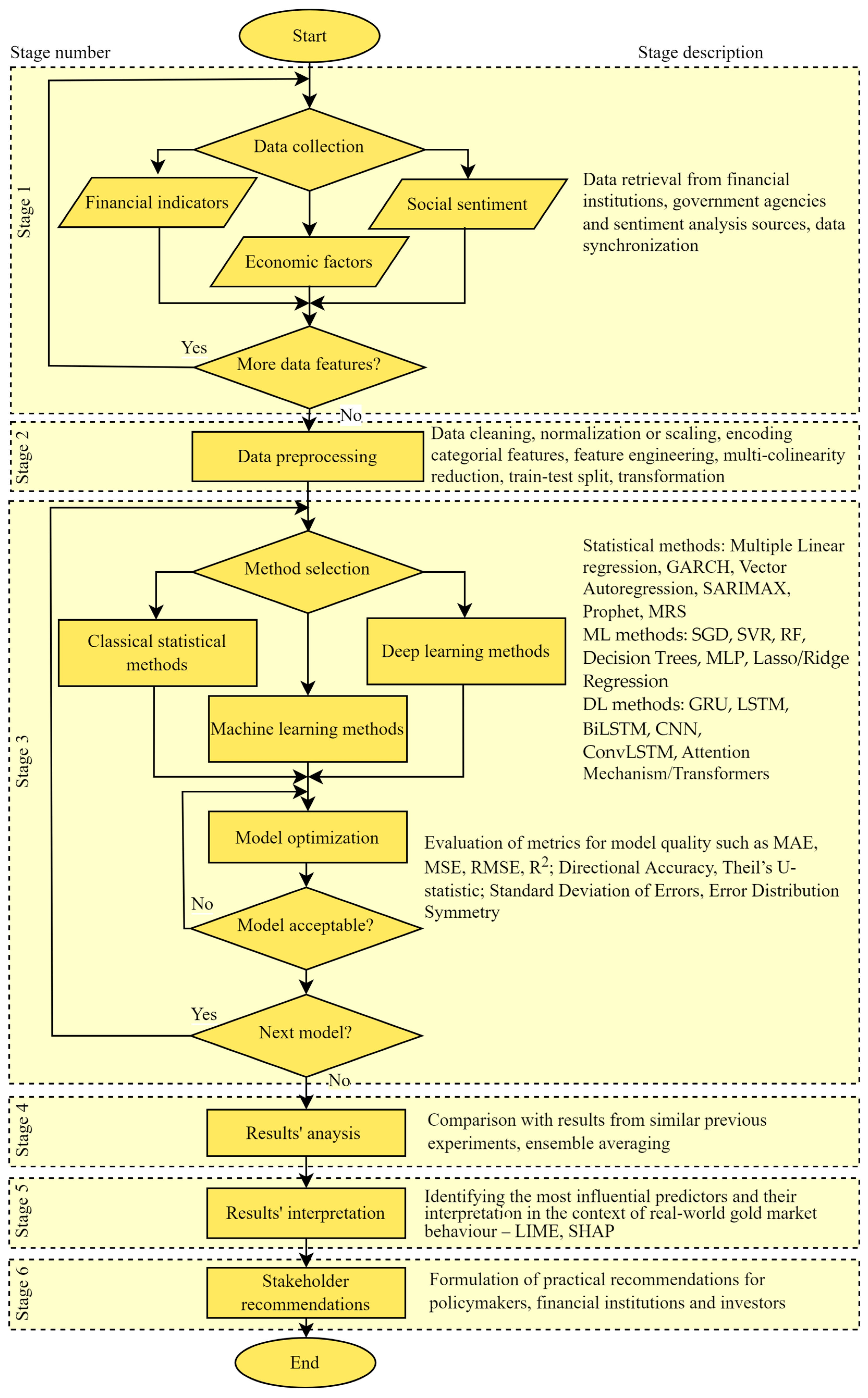
The proposed framework connects three categories of inputs (financial, macroeconomic, and sentiment indicators) with three modelling families (classical statistical techniques, ML algorithms, and DL architectures) (Figure 1). This design captures linear and nonlinear patterns, seasonal effects, and long-range dependencies of diverse gold price prediction factors using the strengths of each approach. Figure 1 presents the flowchart of this hybrid methodology with its six stages.

1.

Data Collection and Integration

Relevant financial indicators, macroeconomic variables, and sentiment measures are gathered from reliable commercial and non-commercial sources (financial data platforms, official economic databases, public sentiment feeds). All variables are synchronised to a common, high-frequency grid—daily and, where available, intraday—to ensure consistency and to provide the large sample sizes required for DL models. The aligned series are then merged into a single dataset for further processing.

2.

Data Preprocessing

The collected dataset is first cleaned and validated. Missing values are imputed or, where appropriate, removed, and outliers are detected and addressed to preserve data integrity. Numerical features are normalised with min-max scaling or standardised, while categorical or sentiment-based inputs are converted through label encoding or other numerical transformations. Optional feature-engineering steps add lag variables, rolling averages, and other constructs that capture temporal dynamics and cross-indicator interactions.

To build the predictor set, a multi-step screening procedure limits multicollinearity and overfitting. The workflow begins with correlation and cross-correlation analysis to probe linear and lagged links between gold prices and candidate variables. Granger causality tests (Granger, 1969) then identify significant lead–lag effects. Markov switching models capture regime shifts and nonlinear dependencies, and ridge regression gauges variable influence in a penalised linear setting. Clustering techniques reveal latent groupings, while VIF checks further reduce collinearity. Wavelet decomposition examines time–frequency relationships, isolating predictors that matter at different horizons. Finally, SHAP values from preliminary ML models quantify each variable’s marginal contribution, providing a robustness check on the preceding steps. Together, these methods yield a predictor set that is both theoretically grounded and empirically validated.

Once the input set is finalised, the data are split chronologically—never randomly—to avoid leakage of future information into model training. Three split strategies are used:

• Simple hold-out (Cerqueira et al., 2020), where the earliest x% of observations form the training set and the most recent (100 − x)% remain an untouched test set.
• Rolling-window validation (Tashman, 2000), in which a fixed-length training window moves forward through time; after each shift the model is retrained, the subsequent short period is forecast, and the error is recorded.
• Expanding-window validation, where the training set grows step by step; each expansion is followed by a short test window and error recording.

Note: Dataset partitioning is required only for the ML and DL models. For each split, scalers, encoders, and other preprocessing transformers are fitted exclusively on the current training data, then applied to the corresponding test data. Each model is subsequently trained and evaluated, ensuring that the assessment reflects real-time forecasting conditions and remains free of information leakage.

3.

Method Selection, Model Configuration, and Validation

At this stage, the prepared dataset is assigned to one of three modelling families. The tasks cover method choice, model construction, and validation. Each model is equipped with its own hyper-parameters: lag orders for econometric methods, kernel or tree settings for ML algorithms, and layer width, learning rate, or dropout for neural networks. Hyper-parameters are tuned strictly within the estimation window grid search for econometric models, random or Bayesian search for ML methods, and early-stopping schedules for DL networks.

Hyper-parameters are optimised strictly within the estimation windows grid search for statistical models, random or Bayesian search for ML algorithms, and early-stopping with dropout schedules for neural networks.

Model validation employs two chronologically ordered approaches, described in Stage 2. Beyond these splits, additional validation approaches—such as walk-forward analysis with expanding windows or fixed rolling windows—can be adopted within the same framework to suit different operational requirements. Forecast accuracy is reported via MSE, MAE, RMSE, and R².

The combination of diverse validation methods and complementary metrics ensures a comprehensive model assessment. This allows us to evaluate model generalization capability and practical applicability across different forecasting scenarios.

4.

Results’ Analysis

After training, tuning, and validation, the models are assessed on multiple criteria. Forecast accuracy is measured with standard error metrics across statistical, ML, and Dl models. Robustness can be evaluated by testing each model during periods of market volatility and external shocks (e.g., major geopolitical events). Diebold–Mariano tests and the MCS procedure can establish formal rankings, offering a rigorous basis for identifying the best-performing models.

The final gold price prediction can be derived either from the best-performing individual model or through a meta-modelling approach such as ensemble averaging, where forecasts are combined and weighted according to model performance metrics, thereby improving robustness and generalization.

5.

Results’ Interpretation

The interpretation of results is crucial for identifying the most influential predictors. Statistical significance tests highlight the impact of financial, macroeconomic, and sentiment indicators on the final predictions. To better understand the output of the ML and DL models used in this framework, model-agnostic interpretability tools can be employed. LIME (Local Interpretable Model-agnostic Explanations) (Ribeiro et al., 2016) and SHAP (Lundberg & Lee, 2017) can be employed because they provide transparent, consistent, and intuitive explanations of black-box model predictions—an important consideration in financial contexts where interpretability and trustworthiness are essential.

6.

Stakeholder Recommendations

Finally, practical recommendations follow directly from the empirical results. Investors and financial institutions are directed to the indicator combinations and forecasting models that deliver the most reliable forecasts for portfolio optimisation and hedging. Policymakers and supervisory authorities receive guidance on the macroeconomic and sentiment indicators that most strongly influence gold prices, information that can refine monetary-policy deliberations and broader financial-stability measures.

To minimize overfitting, the framework employs separation of data and regularization at every modelling stage. All data transformations—scaling, encoding, lag-creation, and feature engineering—are fitted exclusively on the training partition and then applied, without change, to validation or test splits. For classical econometric models, orders and exogenous-lag structures are chosen by information criteria (AIC, BIC) rather than by direct optimisation on the test data. ML algorithms undergo hyper-parameter tuning via time series cross-validation (e.g., rolling-window or expanding-window schemes) to ensure that each configuration is selected based on genuine out-of-sample performance. DL architectures incorporate dropout, L2 weight decay, and early stopping on a held-out validation segment, with training halted once the validation loss ceases to improve. In all cases, the final test block is never consulted until after the model pipeline and hyper-parameters are locked in, providing an unbiased assessment of predictive accuracy.

In summary, the framework ensures a holistic and structured workflow for multivariate gold price forecasting. The accuracy and stability of the resulting models are benchmarked with standard error measures and forecast comparison tests. The obtained rankings show the effective indicators–model combinations, delivering reliable guidance for investment decisions and policy analysis.

4. Framework Verification

This section demonstrates the reliability of the proposed forecasting framework through its application to gold-futures prediction. After fusing a wide array of factors, a feasible subset of input variables is selected. Following the presented workflow, a diverse set of models is then developed, and their performance and stability are evaluated. Achieving acceptable accuracy across these models confirms the framework’s practical applicability.

1.

Data Collection and Integration

The selection of independent variables for gold futures price prediction was grounded in both economic theory and empirical evidence, incorporating financial market dynamics, macroeconomic fundamentals, and sentiment-based influences. Initially, 19 candidate predictors were identified, reflecting three key domains: ten financial market indicators, seven macroeconomic variables, and two sentiment indices.

Table A1. Gold futures and extended set of potential independent factors for their prediction.

Abbreviation	Indicator Name	Description
GC = F	Gold Futures	A standardized contract to buy or sell gold at a predetermined price on a future date; widely used for hedging against inflation, managing risk, and speculating on gold price movements. Available online: https://www.investing.com/commodities/gold (accessed on 20 May 2025)
HG = F	Copper Futures	A contract to buy or sell copper at a future date, often viewed as an economic barometer. Available online: https://www.investing.com/commodities/copper (accessed on 20 May 2025)
CL = F	Crude Oil Futures	A standardized contract for buying or selling crude oil at a set price in the future. Available online: https://www.investing.com/commodities/crude-oil (accessed on 20 May 2025)
MSCI	MSCI World ETF (Global Equity Fund)	An exchange-traded fund tracking a broad global equity index across developed markets. Available online: https://www.investing.com/etfs/ishares-msci-world (accessed on 20 May 2025)
NASDAQ	NASDAQ-100	A global electronic marketplace listing many of the largest technology companies. Available online: https://www.investing.com/indices/nq-100 (accessed on 20 May 2025)
PA = F	Palladium Futures	A futures contract for palladium, a precious metal important in industrial applications. Available online: https://www.investing.com/commodities/palladium (accessed on 20 May 2025)
PL = F	Platinum Futures	A futures contract for platinum, used as both an industrial metal and investment asset. Available online: https://www.investing.com/commodities/platinum (accessed on 20 May 2025)
S&P 500	S&P 500	A market-capitalization-weighted index of 500 leading publicly traded companies in the US. Available online: https://www.investing.com/indices/us-spx-500 (accessed on 20 May 2025)
SI = F	Silver Futures	A contract to buy or sell silver at a future date, reflecting investors’ views on silver prices. Available online: https://www.investing.com/commodities/silver (accessed on 20 May 2025)
US 10Y Treasury	10-Year US Treasury Bond Yield	The yield (interest rate) on the US government’s 10-year bond, a benchmark for global borrowing costs. Available online: https://www.investing.com/rates-bonds/u.s.-10-year-bond-yield (accessed on 20 May 2025)
VIX	Volatility Index	A real-time market index indicating the market’s expectations of 30-day forward volatility. Available online: https://www.investing.com/indices/volatility-s-p-500 (accessed on 20 May 2025)
CPALTT01USM657N	Consumer Price Index	Measures the weighted average of prices of a basket of consumer goods and services. Available online: https://fred.stlouisfed.org/series/CPALTT01USM657N (accessed on 20 May 2025)
CIVPART	Civilian Labour Force Participation Rate	The percentage of the civilian population that is employed or actively seeking employment. Available online: https://fred.stlouisfed.org/series/CIVPART (accessed on 20 May 2025)
EMRATIO	Employment-Population Ratio	The proportion of a country’s working-age population that is employed. Available online: https://fred.stlouisfed.org/series/EMRATIO (accessed on 20 May 2025)
FEDFUNDS	Federal Funds Rate	The interest rate at which depository institutions lend balances at the Federal Reserve to each other overnight. Available online: https://fred.stlouisfed.org/series/FEDFUNDS (accessed on 20 May 2025)
GFDEGDQ188S	US Federal Debt to GDP Ratio	The ratio of total federal debt to the nation’s gross domestic product. Available online: https://fred.stlouisfed.org/series/GFDEGDQ188S (accessed on 20 May 2025)
PSAVERT	US Personal Savings Rate	The proportion of disposable income that households save rather than spend. Available online: https://fred.stlouisfed.org/series/PSAVERT (accessed on 20 May 2025)
UNRATE	Unemployment Rate	The percentage of the total labour force that is jobless and actively seeking employment. Available online: https://fred.stlouisfed.org/series/UNRATE (accessed on 20 May 2025)
GEPUCURRENT	Global Economic Policy Uncertainty Index	Captures the frequency of terms related to economic policy uncertainty across news sources worldwide. Available online: https://fred.stlouisfed.org/series/GEPUCURRENT (accessed on 20 May 2025)
GPRD	Geopolitical Risk Index	Measures the frequency of references to geopolitical tensions in major international newspapers. Available online: https://www.matteoiacoviello.com/gpr.htm (accessed on 20 May 2025)

Note: The indicators in the table are grouped and listed alphabetically within three main categories: financial, macroeconomic, and social sentiment indicators. This structure reflects the classification used in the proposed forecasting framework.

provides a complete list of indicator abbreviations, full names, and descriptions.

From the financial viewpoint, the model includes leading indicators such as continuous commodity futures (Copper, Crude Oil, Palladium, Platinum, and Silver), benchmark stock indices (MSCI World ETF, NASDAQ, and S&P 500), the 10-year U.S. Treasury bond yield, and the Volatility Index (VIX). These indicators reflect investor expectations, global risk perceptions, and market sentiment, and capture the relationships between gold and other strategic assets.

The selection of specific variables was guided by their economic relevance and theoretical linkage to gold market behaviour. For example, Copper Futures (HG = F) are widely used in industry and strongly connected to economic activity, making them a useful proxy for growth expectations. As shifts in copper prices often precede broader economic changes, they can influence gold demand as an alternative investment. Crude Oil Futures (CL = F) are also critical, as rising oil prices lead to higher production costs and inflation, both of which increase investor interest in gold as a hedge. Palladium (PA = F) and Platinum (PL = F), precious metals closely related to gold, reflect broader sentiment shifts in the metals market. Silver Futures (SI = F) typically correlate strongly with gold prices, offering additional insights into market trends. Regarding stock indices, the MSCI World ETF tracks equities from developed economies, serving as a global benchmark. The NASDAQ index reflects the technology sector’s sensitivity to innovation and risk appetite; during uncertainty, gold often emerges as a safer alternative. The S&P 500 serves as a crucial benchmark for the U.S. market, with changes in this index signalling shifts in capital flows that affect gold prices. The 10-year U.S. Treasury yield indicates inflation expectations and monetary policy stances; rising yields typically make non-interest-bearing assets like gold less attractive. Finally, the VIX measures market uncertainty and investor anxiety, with higher volatility often leading to increased gold demand. These financial variables were sourced from the website www.investing.com (accessed on 3 June 2025).

Given the central role of the U.S. in the global economy and gold’s primary denomination in U.S. dollars, the dataset includes seven U.S. macroeconomic indicators linked to inflation, labour markets, interest rates, public debt, and economic growth. The Consumer Price Index (CPALTT01USM657N) tracks inflation and consumer purchasing power, crucial due to gold’s traditional role as an inflation hedge. The Federal Funds Rate (FEDFUNDS), set by the U.S. Federal Reserve, directly affects gold’s attractiveness relative to interest-bearing assets. Three labour market indicators were also included, the Employment–Population Ratio (EMRATIO), Labour Force Participation Rate (CIVPART), and Unemployment Rate (UNRATE), which provide insights into overall economic strength. Economic weakness often increases gold’s appeal as an investment. Additionally, the Personal Savings Rate (PSAVERT), indicating household saving behaviour, was selected; high savings rates may reflect economic uncertainty, prompting investors to seek safer assets like gold. The final macroeconomic indicator, Federal Debt to GDP Ratio (GFDEGDQ188S), measures fiscal sustainability, as high national debt can weaken confidence in a currency and stimulate demand for gold. These official economic indicators were sourced from Federal Reserve Economic Data and the World Bank databases.

To strengthen the model further, two sentiment-based indicators were included. The Global Economic Policy Uncertainty Index (GEPUCURRENT) captures uncertainty regarding global economic policies, directly influencing investor behaviour. The daily Geopolitical Risk Index (GPRD) reflects international tensions and conflicts, typically driving gold demand upward during crises. These sentiment measures were sourced from PolicyUncertainty.com (Baker et al., 2025) and the Geopolitical Risk Index database by Caldara and Iacoviello (Caldara & Iacoviello, 2022) (accessed on 3 June 2025).

To achieve data consistency, all variables were converted to a daily frequency using linear interpolation, especially for macroeconomic factors originally available at lower frequencies. This ensures full dataset synchronization, maintaining accuracy and coherence throughout the modelling process. The collected and synchronized dataset comprises 20 features and 2764 observations.

2.

Data Preprocessing

Following the preprocessing (data cleaning, correlation analysis, multicollinearity diagnostics using VIF scores, and feature importance ranking using ML techniques), a refined set of independent variables was selected.

The analysis of descriptive statistics indicates that most financial variables are reasonably distributed, while certain metals and volatility indices exhibit heavy-tailed behaviour. Macroeconomic and sentiment indicators display structural asymmetries and periodic spikes, suggesting their suitability for regime-switching or interaction-based modelling. VIX shows pronounced non-normality, highlighting the need for careful preprocessing.

Silver is included in the input variable set due to its strong economic alignment with gold as a precious metal and safe-haven asset. Both respond similarly to inflation, geopolitical tensions, and shifts in investor sentiment, and are commonly treated as substitutes in portfolio strategies. Silver is also traded through comparable financial instruments, such as futures and ETFs, and is influenced by similar market forces. Its inclusion can enhance the models’ ability to capture investment-driven dynamics and safe-haven behaviour that are central to gold price movements.

Crude Oil is selected due to its role as a key inflation proxy and macroeconomic indicator; its price movements often reflect global economic conditions and geopolitical tensions, both of which influence gold demand. The U.S. 10-year Treasury yield is also retained, as it represents the benchmark interest rate and reflects investor expectations for inflation and monetary policy—factors that affect the opportunity cost of holding gold. Its economic relationship to the gold price is typically inverse, making it a valuable explanatory variable. The Employment-to-Population Ratio (EMRATIO) is preserved for its ability to capture overall labour market health more effectively than other employment metrics. A lower EMRATIO is often associated with increased demand for gold as a safe-haven asset during periods of economic uncertainty. Lastly, the Federal Funds Rate (FEDFUNDS) is retained as a direct measure of monetary policy. It significantly influences real interest rates and investor behaviour, with rate increases generally leading to downward pressure on gold prices. Each of these variables contributes uniquely to understanding gold price movements and complements the broader macroeconomic and market sentiment context.

GEPUCURRENT (Global Economic Policy Uncertainty Index) is selected for the input variable set due to its strong theoretical and empirical relevance to gold price movements. As a measure of global economic policy uncertainty, it captures shifts in investor sentiment that often drive demand for gold as a safe-haven asset. The variable demonstrates statistically significant relationships with gold in both linear and nonlinear analyses (Granger causality test and Markov switching model) and complements other macroeconomic indicators by reflecting real-time market concerns that are not captured by structural data alone. Its inclusion enhances the model’s ability to predict gold price dynamics under varying economic and geopolitical conditions. To apply the Granger causality test and Markov switching model, we use Python (version 3.12.3) with the grangercausalitytests() function and MarkovRegression() class from the statsmodels library (version 0.14.4).

The inclusion of GPRD is justified based on the results of the polynomial regression, which reveal a significant nonlinear relationship with gold prices. The analysis also shows that moderate increases in geopolitical risk tend to raise gold demand, aligning with gold’s role as a safe-haven asset. However, the negative quadratic term suggests that when geopolitical uncertainty becomes extreme, this positive relationship weakens or may even reverse, indicating that investor behaviour can shift under conditions of severe crisis. These findings highlight that GPRD captures context-dependent effects not reflected in linear models and is particularly valuable for explaining gold price dynamics during periods of heightened geopolitical tension. Therefore, retaining GPRD enhances the model’s ability to reflect real-world investor responses under different market regimes.

The obtained final dataset consists of the following seven independent variables from the three factor groups: Crude Oil Futures (CL = F), Silver Futures (SI = F), US 10Y Treasury Yield; Employment–Population Ratio (EMRATIO), Federal Funds Rate (FEDFUNDS); Geopolitical Risk Index (GPRD), and Global Economic Policy Uncertainty Index (GEPUCURRENT). This subset was chosen based on their statistical significance, predictive power, and economic interpretability. These variables exhibit low multicollinearity, consistent availability throughout the analysis period, and strong theoretical relevance to gold price fluctuations. Although some are originally reported at a lower frequency, their inclusion allows the model to capture a balanced range of influences—from monetary policy and labour dynamics to market volatility and geopolitical risk—thereby supporting more accurate and generalizable forecasting outcomes.

In this stage, we used only the hold-out approach for dataset splitting. The selected dataset comprises eight features, and the observations were split using an 80/20 ratio into training and test sets. All tuning decisions were performed to the training set, and appropriate regularisation techniques were applied to mitigate overfitting. Future work will extend the evaluation to the full range of partitioning and validation schemes outlined in the framework, including cross-validation and rolling-window testing.

3.

Method Selection, Model Configuration, and Validation

SARIMAX, SGD, Prophet, GRU, LSTM, Bi-LSTM, CNN, and ConvLSTM were selected to validate the proposed framework due to their complementary advantages in capturing distinct features of time series data. These methods collectively address linear and nonlinear dependencies, seasonality, trend decomposition, and temporal dynamics—core aspects of gold price behaviour. Their diversity aligns with the structure of the proposed framework, ensuring that each component of the methodology is thoroughly evaluated using multiple methods within each modelling category.

The SARIMAX model is configured with non-seasonal parameters (order = (0, 0, 0)) and disabled seasonal components (seasonal_order = (0, 0, 0, 12)), effectively reducing it to a regression model with exogenous variables—functionally equivalent to ARIMAX. This simplified configuration yielded the best empirical performance in the current experimental setup, likely due to the absence of strong seasonal patterns and the dominance of external macroeconomic factors. Nevertheless, the SARIMAX is retained in full within the modelling pipeline, as it allows for future extensions involving seasonal dynamics and autoregressive behaviour, which may become relevant with longer time series or additional training data. The SARIMAX model is implemented using the SARIMAX class from the statsmodels library (version 0.14.0).

The SGD model is developed using the SGDRegressor class from the scikit-learn library (version 1.3.2). It functions as a linear regression model optimized via stochastic gradient descent. In this configuration, the model minimizes the Mean Squared Error loss (loss = ‘squared_error’), equivalent to ordinary least squares regression solved through iterative updates. Parameter estimation is performed using randomly selected mini-batches from the training data, which allows for significantly faster convergence, particularly in high-dimensional or large-scale datasets. The initial learning rate is set via eta0, and adaptive scheduling mechanisms are used to refine it during training.

The Prophet model (Figure 2) decomposes the gold price into components such as trend, seasonality, holiday effects, and user-defined external regressors. In this implementation, a changepoint prior scale of 0.1 (changepoint_prior_scale = 0.1) is applied to control trend flexibility, balancing generalization with sensitivity to macroeconomic shifts. The model incorporates seven exogenous variables through the add_regressor() function and performs maximum a posteriori (MAP) optimization over the specified priors. Prophet uses automated changepoint detection and applies the L-BFGS algorithm for parameter estimation within a generalized additive model (GAM) framework. No holiday effects or multiplicative seasonality were included, and regressors were kept unscaled to preserve interpretability. The model is implemented via the Prophet class from the prophet library (version 1.1.4).

The GRU model uses a 64-unit recurrent layer followed by dense layers of 64 and 32 neurons. The standard LSTM model contains a single LSTM layer with 64 memory cells, again followed by two dense layers. The Bidirectional LSTM model includes a bidirectional recurrent layer with 64 hidden units (units = 64), followed by two fully connected layers with 64 and 32 neurons, and a final output neuron for regression. The CNN model starts with a Conv1D layer (filters = 64, kernel_size = 3), followed by MaxPooling1D, flattening, and dense layers. The ConvLSTM model captures spatiotemporal patterns using a 2D convolutional recurrent layer with 64 filters (filters = 64) and kernel size (1, 3), followed by flattening and dense layers.

All DL models were implemented using TensorFlow Keras version 2.15.0. The Bi-LSTM was constructed with Bidirectional and LSTM layers; the LSTM model used the LSTM layer; the CNN model included Conv1D, MaxPooling1D, and dense layers; and the ConvLSTM model employed the ConvLSTM2D layer. Each model was trained for 100 epochs using a batch size of 16 and optimized using the Adam algorithm with Mean Squared Error as the loss function.

To minimize overfitting, all preprocessing steps are fitted only on the training data and applied unchanged to test partition. DL hyper-parameters (dropout rate, patience, L2 penalty) are optimised via early stopping. In every case, the test set is consulted only once, after all configurations are fixed.

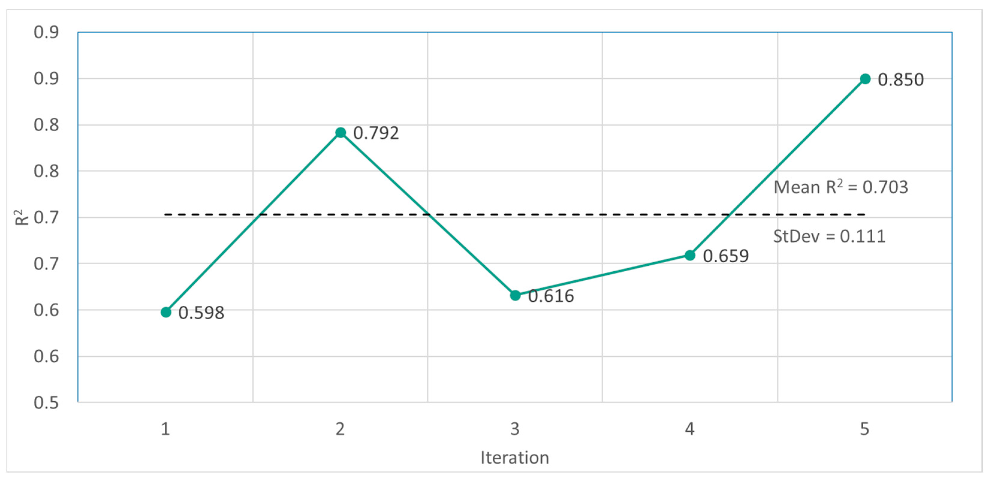
To validate the models, we conducted a stability test aimed at evaluating the consistency of its performance across multiple independent runs. The stability test for the BiLSTM model, based on five independent runs using the same test set (Figure 3), reveals notable variability in its predictive performance as measured by the Coefficient Of Determination R².

Forecast accuracy ranges from 0.598 to 0.850 with a mean R² of 0.703 with a standard deviation of 0.111. Although most runs converge to reasonably similar levels, four out of five exceed an R² of 0.60 and two surpass 0.79, and the observed spread underscores the impact of random weight initializations and training dynamics. These results suggest that while the BiLSTM model is generally robust, employing ensemble methods or repeated training with multiple seeds could further enhance predictive stability.

Note: Due to space constraints, in this stage verification we have included only one chart of actual versus predicted values for the top-performing Prophet model (Figure 2), alongside a stability test chart for the second-best BiLSTM model (Figure 3).

4.

Results’ Analysis

The forecasting results from the obtained models reveal distinct patterns in their ability to capture temporal dependencies (see Figure 4 for the LSTM model) and in their predictive performance on gold futures prices (

Table 2. Forecasting performance of models on the test set.

Model	MAE	RMSE	R2
SARIMAX	148.75	185.31	0.577
SGD	190.96	229.21	0.353
Prophet	76.30	102.34	0.871
GRU	201.07	222.53	0.390
LSTM	129.67	159.05	0.688
BiLSTM	113.65	145.60	0.739
CNN	181.30	227.17	0.364
ConvLSTM	199.03	227.23	0.364

). In this section, we compare each model’s accuracy and evaluate its stability across multiple independent runs to assess robustness under varying initializations and training conditions.

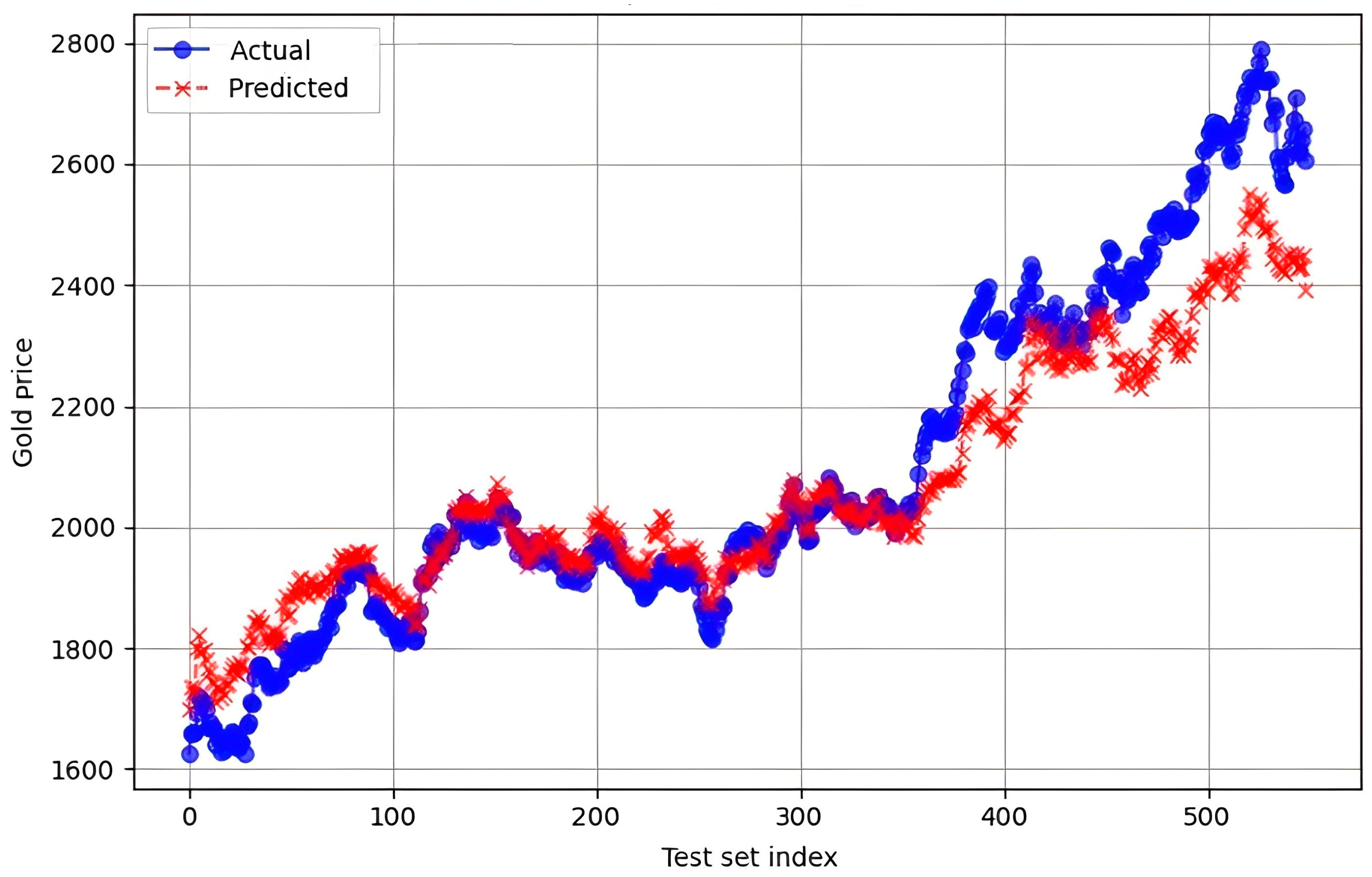
The Prophet model (Figure 2) shows strong predictive performance overall (R² = 0.871) and close tracking of actual gold prices through most of the test period. However, in the last segment (early 2024), the model begins to underestimate gold prices. This decline in accuracy reflects increased market volatility during that time, possibly caused by unexpected changes in interest rates, inflation trends, or geopolitical tensions. Such sudden shifts are harder for the model to capture, especially when they fall outside of established seasonal or trend patterns.

The traditional econometric model, SARIMAX, delivers moderate performance with an MAE of 148.75, RMSE of 185.31, and R² of 0.577. Although it incorporates exogenous variables and captures linear trends, its limited capacity to model nonlinearities and structural breaks constrains its effectiveness. Nevertheless, SARIMAX outperforms several ML and DL models, underscoring its continued relevance when model interpretability is a priority.

In the ML category, the SGD regressor shows lower predictive accuracy (MAE = 190.96, RMSE = 229.21, R² = 0.353). While SGD is computationally efficient and well suited to high-dimensional data, its linear formulation and sensitivity to hyper-parameters reduce its effectiveness in modelling complex, nonlinear patterns typical of financial time series.

Among DL architectures, the BiLSTM model achieves the strongest performance (MAE = 113.65, RMSE = 145.60, R² = 0.739), outperforming the standard LSTM (Figure 4) (MAE = 129.67, RMSE = 159.05, R² = 0.688) and GRU (MAE = 201.07, RMSE = 222.53, R² = 0.390). These results reflect the benefits of bidirectional processing in capturing both past and future dependencies. In contrast, convolutional models such as CNN (MAE = 181.30, RMSE = 227.17, R²= 0.364) and ConvLSTM (MAE = 199.03, RMSE = 227.23, R² = 0.364) underperform, likely due to their limited ability to model long-term sequential dependencies.

Surprisingly, the advanced forecasting model, Prophet, achieves the best overall performance (MAE = 76.30, RMSE = 102.34, R² = 0.871). Its strength lies in capturing structural trend changes and integrating external regressors, which are critical for modelling gold futures influenced by macroeconomic shocks. Unlike DL models that require large datasets and are prone to overfitting in volatile markets, Prophet handles irregularities and limited data more effectively through its additive structure and built-in changepoint detection.

In summary, the model analysis confirms that Prophet and Bi-LSTM offer the highest forecasting accuracy. These models outperform traditional econometric and AI approaches, highlighting the importance of capturing nonlinearity, temporal memory, and structural dynamics—especially when using enriched input features such as macroeconomic indicators and sentiment signals.

5.

Results’ Interpretation

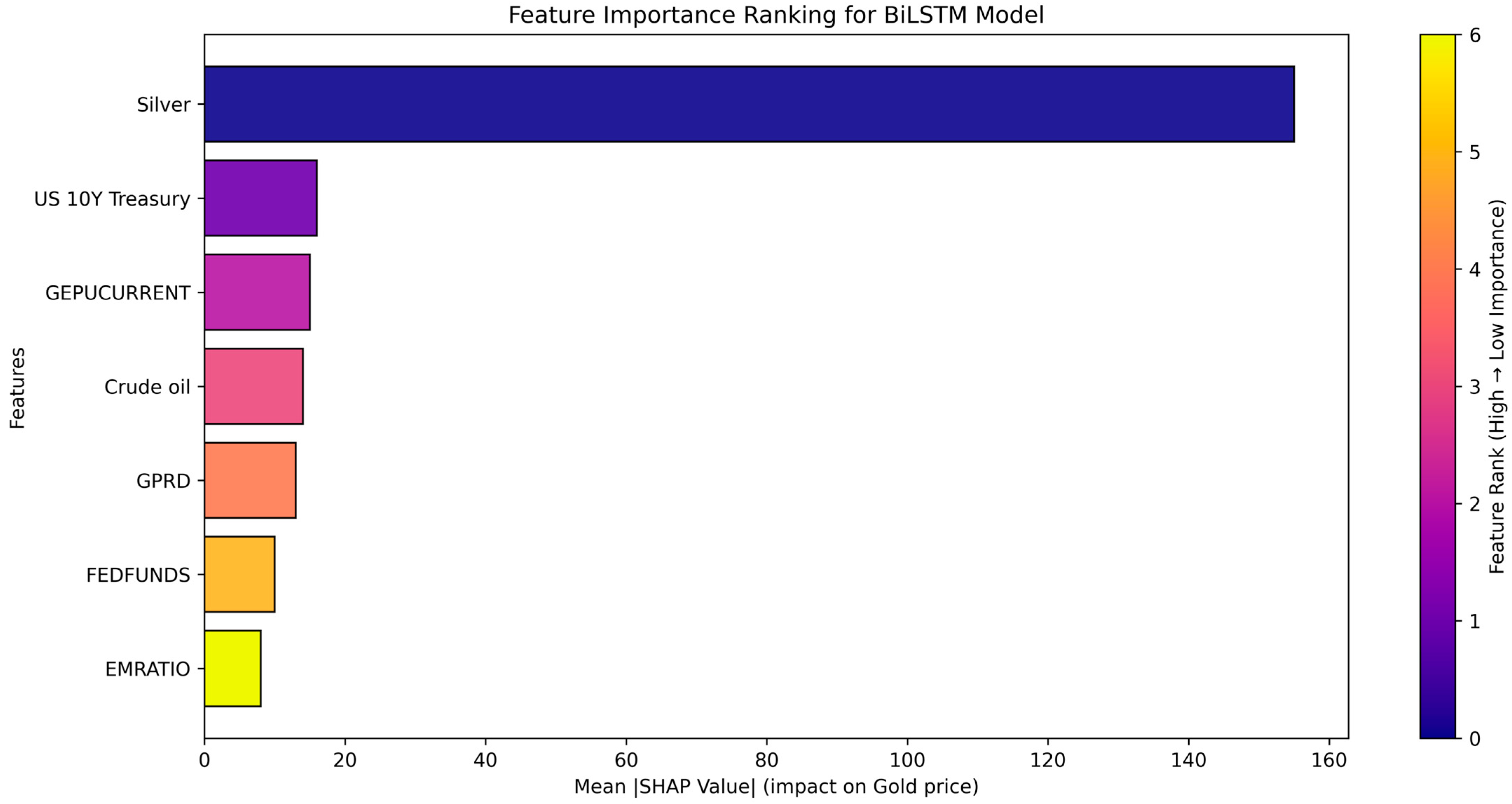
We now proceed to the next stage of the gold price prediction framework—result interpretation—with the goal of understanding the influence of different input variables on model predictions. Prophet and SARIMAX offer built-in interpretability through trend decomposition and regression coefficients. For ML (SGD) and DL (CNN, LSTM, GRU, BiLSTM, and ConvLSTM) models, interpretability can be achieved using post hoc tools like LIME and SHAP, though at higher computational cost. For illustration, we focus on the BiLSTM model, which demonstrated the strongest performance among the DL methods in terms of predictive accuracy and temporal learning capability. Feature contributions within the BiLSTM model are visualized in Figure 5 and Figure 6.

The SHAP results indicate that Silver Futures (SI = F) are the most influential predictor of gold prices, with higher values generally increasing predictions and lower values reducing them. Other important variables include macroeconomic uncertainty measures such as the GEPUCURRENT and the GPRD, reinforcing gold’s role as a safe-haven asset. Additional contributors such as crude oil prices, interest rates (US 10Y Treasury, FEDFUNDS), and the EMRATIO demonstrate moderate yet context-dependent effects. The presence of both positive and negative SHAP values for individual features reflects the model’s ability to capture nonlinear and interaction-driven patterns typical in financial time series.

6.

Stakeholder Recommendations

Based on the forecasting results and model interpretations, stakeholders in gold futures markets, such as investors, analysts, and policymakers, can be advised to prioritize models that offer both strong predictive accuracy and interpretability (in our case study—Prophet and BiLSTM). The SHAP analysis highlights the most influential predictors, indicating that closely monitoring these variables can enhance decision-making. Investors and traders may use the recommended models for dynamic portfolio adjustments, while policymakers can leverage the insights to better anticipate the financial effects of macroeconomic and geopolitical developments. Ensemble forecasts that combine linear and DL models are also recommended for producing robust, context-sensitive predictions that capture both trend shifts and nonlinear dependencies.

5. Discussion

Our experimental results can be compared with those of similar previous studies using several criteria: evaluation metrics, forecast accuracy, computational cost, and interpretability. Regarding evaluation metrics, some studies assess directional-classification tasks, reporting accuracy, F1-score, and AUC rather than regression measures (Hajek & Novotny, 2022; Mamoudan et al., 2023). This choice reflects that trading decisions often depend on up-versus-down moves, not precise price levels. Moreover, a ten-month, highly volatile sample makes classification more stable than point forecasting (Mamoudan et al., 2023). All other studies—including ours—predict continuous prices, so regression performance metrics remain the appropriate performance metrics.

In terms of forecast accuracy, on our multivariate, daily frequency gold futures dataset, Prophet, BiLSTM, and LSTM achieved the best performance, with R² values of 0.871, 0.739, and 0.688, respectively. While some deep hybrid models show higher values—ICEEMDAN–CNN–CBAM–LSTM (Liang et al., 2022) reports R² ≈ 0.98 and BiLSTM (Zangana & Obeyd, 2024) R² = 0.95—these models use univariate or narrowly engineered inputs, respectively. Despite their theoretical capacity to model nonlinear and sequential patterns, our GRU, CNN, and ConvLSTM models underperformed in terms of predictive accuracy (R² = 0.39, 0.364, and 0.364, respectively). Several factors may account for this. First, DL models generally require large, high-quality datasets to generalize well; in our case, the sample size, while sufficient, may not have fully supported the depth and complexity of these architectures. Second, our choice to avoid computationally intensive preprocessing techniques such as signal decomposition may have limited the models’ ability to extract meaningful temporal features. Third, the use of standardized hyper-parameter tuning across all models, rather than model-specific optimization, may have resulted in suboptimal configurations. Lastly, the fused multivariate input structure, while rich in information, may have introduced noise or redundancy that obscured the signal patterns these deep models are best suited to detect.

The next comparison criterion is computational efficiency. Prophet trains in seconds on a CPU, SARIMAX in minutes, and BiLSTM (64 units, 100 epochs) converges in under 10 min on a standard GPU. In contrast, complex architectures like the triple-network pipeline (Liang et al., 2022) or the metaheuristic-optimized CNN–BiGRU (Mamoudan et al., 2023) require significantly more GPU time, making them less suitable for real-time or daily retraining scenarios.

Regarding interpretability, Prophet and SARIMAX offer direct transparency through built-in trend decomposition and regression coefficients. For ML and DL models, SHAP is required to provide post hoc explanations. Among reviewed studies, only Hajek and Novotny (2022) (using fuzzy rule-based systems) and Zangana and Obeyd (2024) (using SHAP) explicitly incorporate interpretability tools, offering a comparable level of transparency. Most other hybrid approaches prioritize prediction accuracy at the expense of model explainability.

Previous studies commonly follow four methodological strategies: signal decomposition combined with deep networks, metaheuristic hyper-parameter tuning, input fusion, and post hoc explainability. In verifying our framework, we emphasize the latter two—a fusion of financial, macroeconomic, and sentiment data, alongside explainable AI techniques—while deliberately excluding resource-intensive approaches such as signal decomposition and evolutionary optimization. This design choice prioritizes interpretability, scalability, and practical implementation over maximizing predictive accuracy. Consequently, although some of our advanced models (e.g., Prophet, BiLSTM, LSTM) show competitive performance, they may not fully capture the most intricate temporal dependencies compared to highly optimized or decomposed pipelines. Still, the trade-off supports faster retraining, more transparent model behaviour, and broader applicability in real-world forecasting contexts.

6. Conclusions

This study introduces a conceptual framework for forecasting gold futures that combines classical econometric methods with modern ML and DL techniques. It integrates a variety of financial, macroeconomic, and sentiment indicators into a unified workflow, enabling the capture of hidden and complex nonlinear patterns in price dynamics. A well-structured variable selection process helps identify some of the most promising input variables. The experimental results confirm the effectiveness of the proposed holistic methodology in forecasting gold prices and uncovering the most influential factors.

The framework contributes to existing research by showing how the combination of heterogeneous inputs and diverse modelling approaches can support both accurate and interpretable financial time series forecasts. It bridges the gap between transparent, rule-based models and high-capacity neural networks by incorporating explainability techniques, enabling nuanced insights into variable importance—even within complex DL architectures. An additional internal variable selection procedure refines the final input set, reducing noise and redundancy, while the optional meta-modelling component enhances predictive robustness by synthesizing outputs from multiple models. This makes the framework well suited for both academic analysis and practical implementation.

The obtained results provide practical guidance for stakeholders. The ability to identify volatility regimes, evolving macro-financial relationships, and key predictive signals supports more informed portfolio management, policy formulation, and risk mitigation. In particular, the strong and stable performance of certain models developed within the proposed framework underscores their suitability for operational forecasting systems that require both accuracy and interpretability. Overall, the study emphasises the importance of adaptive and transparent forecasting tools in today’s increasingly complex and data-driven financial landscape.

This study has several limitations: (1) the framework relies solely on historical data, excluding real-time inputs, which could enhance predictive performance; (2) the macroeconomic variables in the dataset are available at lower frequencies and require interpolation, potentially introducing noise; (3) the selection of independent variables in the validation phase does not follow a formal optimisation procedure; (4) although multiple models were evaluated, hyper-parameter tuning was applied in a standardised fashion, limiting the potential for model-specific fine-tuning; and (5) evolving market dynamics necessitate ongoing model retraining and drift detection to sustain forecasting accuracy over time.

In the future, we plan to explore the integration of multimodal inputs, combining structured time series data with real-time textual streams. These streaming sources could be analysed using large language models to extract social sentiment and align it with temporal data via attention mechanisms or transformer-based architectures. Additionally, incorporating transfer learning techniques, such as domain adaptation or fine-tuning pre-trained forecasting networks, may enhance model generalisation across different time periods and geographic contexts. Finally, expanding the current framework to support comparative studies involving other commodities or major currencies could deepen insights into interconnected financial systems and promote more adaptive, stable, and informed decision-making in commodity finance.