The Impact of Intangible Capital on Firm Profitability in the Technology and Healthcare Sectors

Abstract

The aim of the present study is to assess the impact of structural capital intensity and utilization on firm profitability in an international setting: the European Union countries, plus Norway, Switzerland and the United Kingdom. The indicators are calculated based on financial data downloaded from the Refinitiv Eikon database. Two financial ratios are used as proxies for the intensity and utilization of structural capital. The balanced panel consists of 625 companies from 25 countries, over the period from 2013 to 2022. The panel includes financial information on two industries that are considered innovation-oriented, namely technology and healthcare. Alternative model specifications are proposed to test the robustness of the basic model, including dynamic models (with lagged dependent variables). The present study indicates that a higher proportion of structural capital (intangible assets, excluding goodwill) is a negative factor for company profitability in the technology and healthcare sectors. There is no indication that a more intense use of intangible assets and more investments in R&D positively contribute to company profitability in the respective industries, for a large sample of listed companies. A higher proportion of intangible assets, as reported in financial statements, is possibly related to inefficiencies in the management of structural capital. The inverse relationship between profitability and investments in intangible assets is likely due to failures in cost accounting. Limitations and future research propositions are provided in the conclusions.

1. Introduction

When considering innovation-oriented sectors, value creation is determined primarily by the effective use of intangible assets (Chowdhury et al. 2019). However, intangible assets, in particular, and intellectual capital, in general, are often omitted from accounting and finance research (Clausen and Hirth 2016). This is because most authors agree that accounting numbers do not reflect the size and importance of intellectual capital (Ahmad 2023). Furthermore, it is believed that the most important components of intellectual capital cannot be reliably measured in monetary terms (Krstić et al. 2023). In particular, structural capital is the term given to intangible assets and other elements in the model proposed by Moon and Kym (2006). From another perspective, structural capital is “a set of procedures, standards, systems, routines, rules, and so on, that together make up the organizational system” (Novas et al. 2017, p. 292). By focusing on structural capital, the present research seeks to narrow down the measurement dilemma regarding intangibles and investigate the impact of structural capital on financial performance, in a replicable setting (i.e., using financial data from Refinitiv).

Structural capital is a conglomerate of infrastructure elements such as intellectual property, internal processes and procedures, information systems, research and development investments, and, more generally, knowledge-related assets (Moon and Kym 2006; Nguyen 2023). A readily available approximation is the size of intangible assets, excluding goodwill. Under internationally recognized accounting standards, intangible assets are reliably measured but with a high degree of accounting conservatism (Butt et al. 2023). Research and development (R&D) expenditure is similarly governed by strict rules regarding recognition and measurement during the development of new products and services. Although this measurement is imperfect, it is the most reliable and comparable method to assess structural capital without resorting to interpretations and approximations (Marzo 2022; Marzo and Bonnini 2023).

Intangible assets are strategic resources used in operational activities and developed by investing in R&D (Clausen and Hirth 2016). Therefore, a higher proportion and increased utilization of such resources are expected to provide a competitive advantage to the firm and lead to superior financial performance (Rahman and Liu 2023). By applying the calculation model proposed by Pulic (2004), previous authors found a positive effect of structural capital efficiency on financial performance in different industries: banking and insurance (Chen et al. 2014; Nawaz and Ohlrogge 2023), tourism (Sardo et al. 2018), healthcare (Scafarto et al. 2023; Tiwari 2022), transportation (Rahman and Liu 2023) and listed firms in general (Kasoga 2020; Katona 2018; Nguyen 2023). The research setting in previous studies was often limited to one country: China (Rahman and Liu 2023), Germany (Nawaz and Ohlrogge 2023), India (Gupta et al. 2023; Tiwari 2022), Hungary (Katona 2018), Malaysia (Chen et al. 2014), Portugal (Sardo et al. 2018) and Tanzania (Kasoga 2020). In an international context, the study of Scafarto et al. (2023) analyzed the relationship between structural capital efficiency in 193 listed healthcare firms from 12 European Union (EU) countries over the period 2017–2021.

The aim of the present study is to assess the impact of structural capital intensity and utilization on firm profitability in an international setting, namely, EU countries plus Norway, Switzerland and the United Kingdom. All listed companies in these countries apply convergent financial reporting standards. The indicators are calculated based on financial data downloaded from the Refinitiv Eikon database. Two financial ratios are used as proxies for the intensity and utilization of intangible assets. The panel data comprise 10 years and 25 countries. Most importantly, the balanced panel includes information on two industries that are considered innovation-oriented, namely technology and healthcare. Alternative model specifications are proposed to test the robustness of the basic model, including dynamic models (with lagged dependent variables) and the generalized method of moments (GMM). These statistical solutions are expected to open up new avenues for research beyond single-country investigations and controversial indicators (Iazzolino and Laise 2013; Marzo 2022; Ståhle et al. 2011).

The contributions of the present study are twofold. First, the proportion and utilization of structural capital are strictly defined as the proportion of intangible assets and the expenditure related to intangible capital creation and utilization. These proxy variables go against the tradition of using the efficiency indicators proposed by Pulic (2000, 2004). The present methodological solution is superior because it clearly connects the studied phenomenon with the measurement instrument. Second, the results of the study draw attention to potential inefficiencies in the utilization of intangible assets and the incongruence between management accounting and structural capital measurement. Accounting conservatism is a double-edged sword on the topic of intangibles: it favors reliability to the detriment of relevance. This assertion is supported by the results of the present study.

The structure of the paper is as follows. The literature review clarifies the terminology in the domain and introduces the two hypotheses of the study. The methodology presents the variables and regression models (basic and alternative tests). The sample description and econometric methods are also detailed in the methodology section. The results section starts with the presentation of descriptive statistics and moves on to the estimation of the base model and several alternative specifications for robustness tests. Each section of the results is clearly linked to the regression models introduced in the methodology section. The discussion and conclusions present the link to previous findings and managerial implications. Alternative explanations of the results are introduced to the reader. Several limitations are enumerated, in addition to ideas for future research.

2. Literature Review

Intangible assets can be viewed from a wide perspective or from a narrow perspective. From a wide perspective, intangible assets refer to intellectual capital and comprise resources that are valuable, rare, inimitable and non-transferable (Kristandl and Bontis 2007). The wide perspective is linked to the resource-based theory, a management theory stating that competitive advantage is based on strategic resources, including intangible assets (Chu et al. 2023). In this perspective, intangible assets are supported by core competencies such as information technology, human resources management, knowledge management, innovation capacity and organizational culture (Moon and Kym 2006). The resource-based theory highlights the unique and strategic characteristics of intangible assets (Ashraf et al. 2023), but such assets can also be reproducible, sellable and of relatively little value. From a narrow perspective, intangible assets are recognized in financial accounting according to a set of principles and rules, irrespective of their cost, rarity or transferability (Zéghal and Maaloul 2011).

From the accounting perspective, intangible assets are long-term (non-current) assets without physical substance that are used in the current operations of the entity in the production process or supply of services, for rental or administrative purposes (IASB 2014). These assets are acquired or created by the enterprise, recognized in accounting, amortized and fully controlled by the entity. The usual types of intangible assets are patents, copyrights, customer lists, software, licenses, franchises, marketing rights, exploitation quotas, etc. If these are acquired, their recognition is straightforward. When intangible assets are generated within the entity, their costs must be identified. Any of the elements on the list above can be recognized separately, with a market value apart from the entity, and can potentially be sold. However, goodwill is a specific type of intangible asset. Goodwill is the difference between the price paid to acquire an entity and its book value of equity. Therefore, it cannot be evaluated and sold separately from the enterprise. In the following discussion and methodology, intangible assets do not refer to goodwill.

In many situations, intangible capital is equated with technological and innovation capital (Feleagă et al. 2013; Fernández et al. 2000). These resources may be created, perfected and expanded through research and development (R&D) activities (Katona 2018). Knowledge capital is another synonym of intangible capital, encompassing patents, formulae, blueprints, engineering specifications and other intellectual products that can be protected by law (through patents). The recognition of patents is in line with the accounting definition of organizational assets, as they are expected to generate future economic benefits in terms of marketable products or services. Some intangible resources are never recognized in the accounting system, such as brand equity, stakeholder relations, human capital, innovation capacity, work efficiency and marketing expenditure (Butt et al. 2023). According to the accounting standard IAS 38, research expenditure is disclosed in the income statement if the technical feasibility of completing a research project is not yet demonstrated. R&D projects can be risky, complex, difficult to monitor and inherently uncertain (Norkio 2023). Therefore, it is difficult for companies to fully internalize their R&D investments (Dai et al. 2022). However, the restrictions on recognizing internally generated intangible assets tend to distort business valuation and compromise the true and fair view of the financial statements (Fontana et al. 2019).

The concept of “structural capital” is closely related to knowledge and organizational performance (Faraji et al. 2022). This concept was employed by Pulic (2004) as a component of intellectual capital. According to Moon and Kym (2006), structural capital refers to the synergy of organizational processes, information systems, intellectual property and “culture”. It is obvious that structural capital provides infrastructure support to employee performance (Chowdhury et al. 2019). Knowledge is also an integral part of structural capital (Chu et al. 2023), but the accounting perspective demands that knowledge-related assets be measured reliably. From another perspective, structural capital encompasses total R&D expenses (Gupta et al. 2023), but R&D activity is not immediately recognized as an asset in the statement of financial position (Zéghal and Maaloul 2011). Some elements of structural capital, such as information systems, procedures and processes, may not be recognized in accounting if developed internally (Krstić et al. 2023). All of these elements are more than just purchased software, which is immediately recognized in accounting and amortized. Therefore, the general understanding is that “structural capital” encompasses more than just intangible assets and R&D expenditure, but that this construct cannot be comprehensively measured using conservative accounting rules (Marzo and Bonnini 2023).

Following the conceptualization of Molloy et al. (2011), resource-based theory is the foundation for testing the impact of intangible capital on firm performance. Intangible assets are linked to value creation logic because they reflect the firm’s strategy, value proposition, products and services and efficiency goals. Intangibles and R&D are embedded in value chains (Porter 2001) because they support the transformation of capital, human effort, energy and knowledge into products and services. Most of the components of structural capital (routines, capabilities, information systems, trademarks, copyrights) are difficult to imitate by competitors. Structural capital contributes to performing operational and administrative activities, thus improving employee productivity and driving revenue growth (Rahman and Liu 2023). Procedures, know-how, databases and processes are the foundation for maintaining long-term relationships with key stakeholders that shape the financial success of the company (Sardo et al. 2018). Therefore, structural capital has a synergistic relationship with other components of intellectual capital such as human capital (talent, skills and expertise) and relational capital (relationships with customers, suppliers, value chain partners or other direct counterparties).

In the technological realm, structural capital encompasses infrastructure and processes that are vital for the functioning of enterprises. Some examples are machine-to-machine communications, cloud computing, big data and predictive analytics, generative algorithms based on artificial intelligence, cross-platform integration and blockchain capabilities (Scafarto et al. 2023). R&D expenditures are recorded by companies that test new technologies and innovative solutions in a dedicated research department (Ahmad 2023). The disclosure of R&D expenditure is a signal that the company engages in continuous learning and seeks to develop innovative products and services, while expanding the internal knowledge base (Ahmad 2023; Chowdhury et al. 2019). Even when these expenses are not capitalized, R&D expenditures contribute to knowledge accumulation and increased productivity at the micro, sectoral and macro levels (Dai et al. 2022). A visual summary of accounting elements that are assigned to structural capital is provided in Figure 1.

The present research focuses on the relationship between intangible (structural) capital utilization and company profitability. In this regard,

Table 1. A summary of previous empirical results from the relevant literature.

Study	Industry	Countries	Sample (Firms)	Dependent	Predictor	Relationship 1
Ahmad (2023)	All	US	6019	ROA, ROE, MB	Innovation capital efficiency	All: + (sig.)
Ashraf et al. (2023)	Hospitality	18 EU countries	42,516	ROA, AG	Structural capital = working capital turnover	ROA: − (sig.) AG: + (sig.)
Chowdhury et al. (2019)	Pharma	Bangladesh	23	AT, ROA, ROE, MB	Structural capital efficiency	All: n/s
Chu et al. (2023)	Technology	China	44	ROA	Invention patents	+ (sig.)
Dancaková et al. (2022)	All	Germany, France, Switzerland	250	TQ	Intangible assets intensity	n/s
Duho (2022)	Not specified	West African countries	59	ROA	Structural capital efficiency	+ (sig.)
Gupta et al. (2023)	Pharma	India	82	ROA, ROE, ROS	Structural capital efficiency	ROA, ROE− (sig.) ROS: n/s
Kasoga (2020)	Manufacturing	Tanzania	22	ROA, AT, SG, TQ	Structural capital efficiency	All: + (sig.)
Katona (2018)	7 industries	Hungary	36,801	Firm production	Technological capital	1996–2005: − (sig.) 2005–2014: + (sig.)
Krstić et al. (2023)	Not specified	International (global brands)	36	ROA, RUE	Efficiency in the use of intangible assets	All: + (sig.)
Marzo and Bonnini (2023)	All	Italy	126	ROA, ROE, MB	Structural capital efficiency	ROA 2018: n/s ROE 2018: + (sig.) MB 2018: n/s
Meles et al. (2016)	Banks	US	5749	ROA, ROE	Structural capital efficiency	All: n/s
Nawaz and Ohlrogge (2023)	Banks	Germany	1 (60 years)	ROA, ROE	Structural capital efficiency	All: + (sig.)
Nguyen (2023)	Services	Vietnam	Not specified	ROE	Structural capital efficiency	Small firms: n/s Large firms: + (sig.)
Radonić et al. (2021)	Technology	Serbia	101	ROA, ROE	Structural capital, innovation capital	+ (sig.)
Rahman and Liu (2023)	Transportation	China	76	ROA, ROE, AT	Structural capital efficiency	All: n/s
Sardo et al. (2018)	Hotels	Portugal	934	ROA	Structural capital = working capital turnover	+ (sig.)
Scafarto et al. (2023)	Healthcare	EU	193	ROA	Structural capital efficiency	+ (sig.)
Tiwari (2022)	Healthcare	India	84	ROA	Structural capital efficiency	+ (sig.)

¹ Relationships indicated by a sign +/− are significant at conventional levels. Non-significant relationships are indicated as n/s. Abbreviations for financial performance variables are as follows: return on assets (ROA), return on equity (ROE), return on sales (ROS), market-to-book ratio (MB), asset growth (AG), asset turnover (AT), sales growth (SG), Tobin’s Q (TQ), resource use efficiency (RUE).

presents a summary of empirical results from the literature. From the list of predictors in each relevant study, only intangible (structural) capital was selected. Most studies use the indicator “structural capital efficiency” based on the proposal by Pulic (2004). This proxy is based on a residual value calculation, where the structural capital of the company is equal to the difference between the value added and wage expenses (which are equivalent to human capital). Structural capital efficiency is the ratio of structural capital to value added, while value added is the sum of operating profits, employee costs, depreciation and amortization. On a closer look, structural capital is equal to earnings before interest, tax, depreciation and amortization, also known as EBITDA (Marzo and Bonnini 2023). Therefore, it is apparent that structural capital efficiency, as calculated by Pulic (2004), is not a good proxy of intangible capital efficiency, because it has no factual connection to the financial elements classified as intangible assets. However, structural capital efficiency has been extensively used in the literature (see Table 1), despite its theoretical drawbacks (Marzo 2022).

Table 1 shows that the literature is dominated by the model proposed by Pulic (2000, 2004). Very few authors have tried to suggest other solutions for the measurement of structural capital, despite the obvious problem of equating intangible capital with EBITDA. Ashraf et al. (2023) used working capital turnover as a proxy of structural capital. The premise is that working capital turnover is an indicator of operational efficiency, shorter operating cycles, and better firm performance. However, this indicator has no direct connection to the utilization of intangible assets (i.e., patents, copyrights, trademarks and databases). Chu et al. (2023) chose the total number of invention patents acquired by the company in a year, which is closer to the concept of intellectual property but does not provide any monetary values for such investments. Dancaková et al. (2022) proposed the indicator that is closest to the domain of intellectual capital, namely intangible asset intensity as the ratio between the book value of intangible assets and the book value of total assets. A modified version of this indicator will also be used in the present study.

The current study relies on financial information that is immediately available from the financial statements of the enterprises. However, a limitation of this approach is that the value of net intangible assets contains only a small fraction of a company’s structural capital (Clausen and Hirth 2016). For this reason, the utilization of intangible capital is proxied by the amortization of intangibles and R&D expenditures. These values are indicators of the use of intangible assets and the firm’s spending on knowledge creation (Clausen and Hirth 2016). Net intangible assets, amortization and R&D expenditures point to different facets of the same phenomenon, namely the company’s dependence on intangible capital. The prevalence and utilization of structural capital, as well as R&D expenditures, are expected to have an impact on corporate financial performance (Dai et al. 2022; Nawaz and Ohlrogge 2023; Rahman and Liu 2023). The following hypotheses will guide the present empirical investigation:

H₁. 

A higher proportion of structural capital leads to higher corporate profitability.

H₂. 

Increased intangible capital utilization leads to higher corporate profitability.

3. Methods and Sample

3.1. Variable Descriptions and Model Specifications

The present research relies on financial accounting information to explore the relationship between intangible capital and company profitability. The solution adopted was to avoid the indicators proposed within the value added intellectual coefficient (VAIC) model (Marzo 2022; Pulic 2000, 2004) and rely on financial ratios that have a straightforward interpretation. Moreover, all companies in the sample apply the International Financial Reporting Standards (IFRS) or the US Generally Accepted Accounting Principles (GAAP), which means that the financial indicators are determined based on a common set of principles. A simple representation of the proposed model and variables is shown in Figure 2, in relation to the hypotheses. As indicated below, intangible capital variables do not refer to intellectual capital efficiency (as in the VAIC model) but to intangible capital prevalence and utilization.

Company profitability (dependent variable) is proxied by three indicators, which are expected to be highly correlated:

• Basic earnings power (BEP) illustrates the capacity of the firm to generate profits before tax and debt service, in relation to total assets. BEP is comparable across various tax conditions and levels of financial leverage, so that it is a financial ratio that is still relevant in an international comparison. BEP can be positive or negative depending on the sign of numerator (earnings before interest and tax). This indicator has been used before in a similar model by Tiwari (2022).
• Return on assets (ROA) shows how profitable a company is in relation to its total assets. ROA is a financial performance ratio which is frequently used in accounting research as a dependent variable, while being sector-specific. This indicator is calculated starting from net income but excluding extraordinary (one-time) elements that could influence financial performance (such as mergers or divestments). ROA can be positive or negative, depending on the sign of the numerator (net income). This profitability indicator has been used in several articles testing similar models (Chowdhury et al. 2019; Rahman and Liu 2023; Sardo et al. 2018; Scafarto et al. 2023).
• Return on equity (ROE) is a financial performance indicator in relation to net assets (i.e., total assets minus total liabilities). Shareholders’ equity is a residual amount that can be positive or negative, depending on the size of the total liabilities compared to total assets. If net income is a loss and total equity is negative, ROE becomes positive. Database cleaning solves this situation by removing entries with negative shareholders’ equity. This profitability indicator has been used in several articles testing similar models (Chowdhury et al. 2019; Rahman and Liu 2023; Scafarto et al. 2023).

The main predictors are two indicators of intangible resource capitalization and utilization, respectively, that are not expected to be correlated:

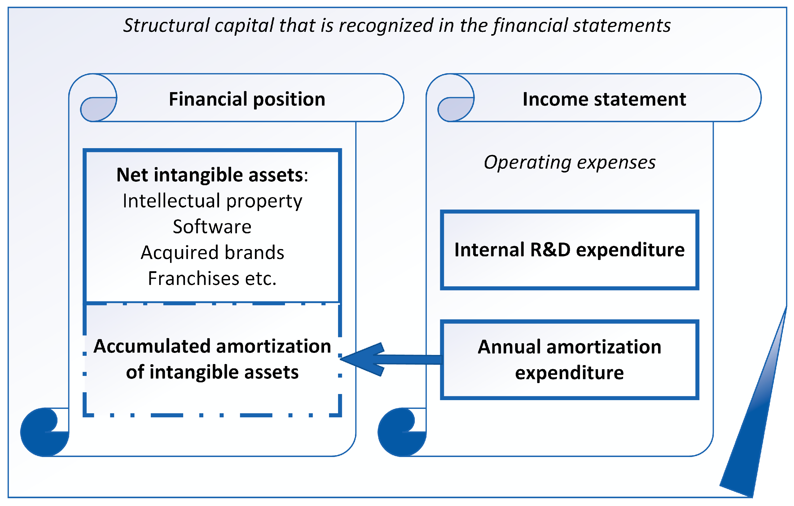
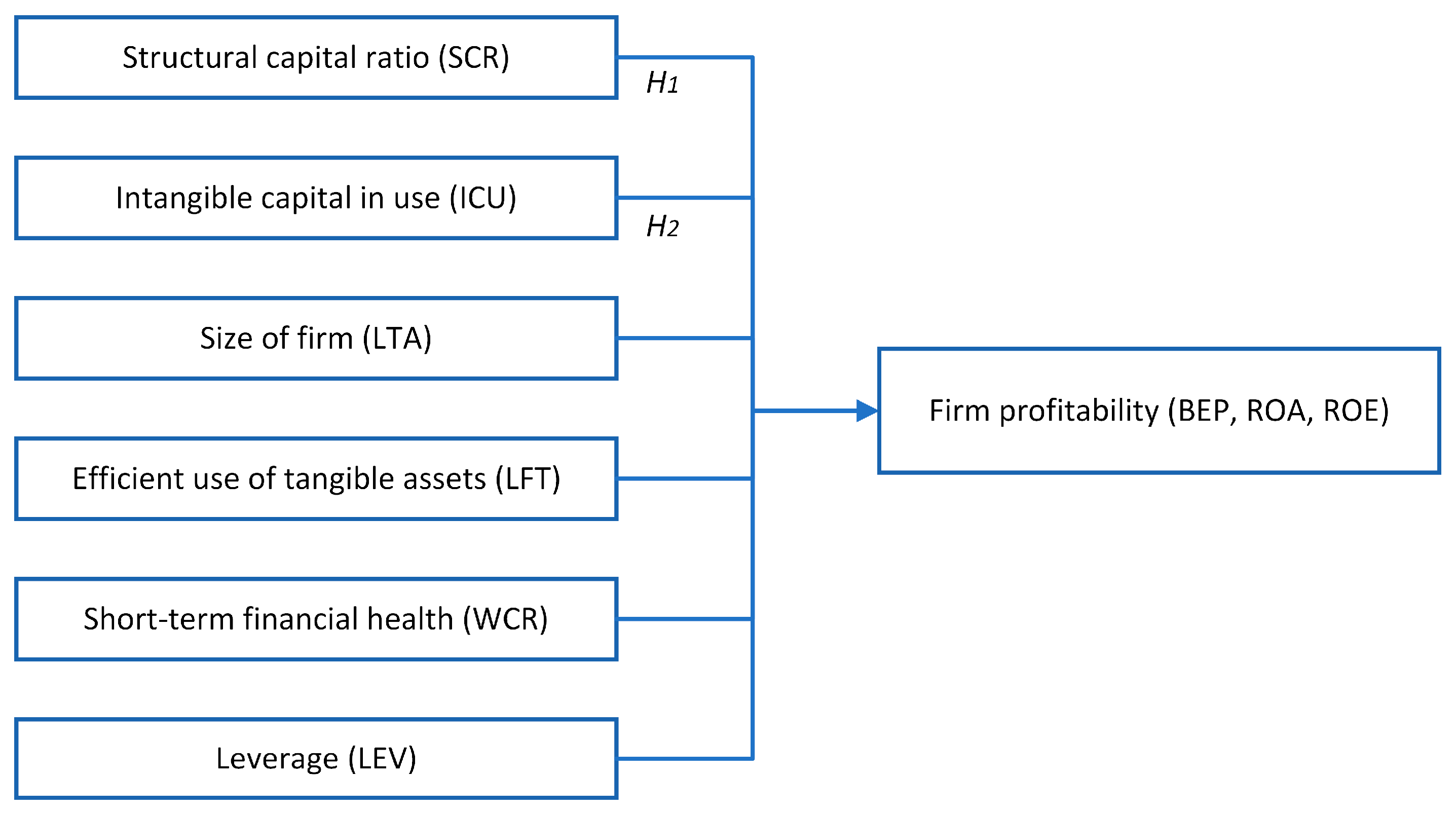
• The structural capital ratio (SCR) is calculated as the proportion of intangible assets (excluding goodwill) to total non-current assets (net of depreciation and amortization). This ratio shows the degree of reliance on intangible assets during operations. This ratio is a snapshot at year end, after the utilization of these assets. From another perspective, it shows the proportion of intangible assets that are available for use during the next financial year. Therefore, SCR at the end of year t is expected to have an effect in the t + 1 period.
• Intangible capital in use (ICU) is the ratio of intangible asset-related expenses to total operating expenses. It shows how much intangible capital (if quantified) was used during the year, in relation to the use of the entire set of company resources. The ICU is expected to have an immediate effect on profitability, but also a delayed effect because intangible capital is an investment. Intangible capital in use captures a different economic reality than SCR because it does not strictly refer to capitalized resources, but also to expenditures that may not appear on the balance sheet. The ICU depends on the correct classification of R&D expenditures according to the IFRS or US GAAP.

The following control variables are introduced to capture other aspects of company efficiency and performance:

• Company size (LTA), calculated as the natural logarithm of total assets, is a control variable frequently used in similar models (Chowdhury et al. 2019; Rahman and Liu 2023; Sardo et al. 2018; Scafarto et al. 2023; Tiwari 2022). It is expected that larger companies are different in terms of their profitability compared to smaller companies. This variable isolates this effect.
• Fixed assets turnover (LFT) indicates the efficiency in the use of property, plant and equipment (PPE). This indicator shows how tangible non-current assets are used by the company, distinct from intangible capital. Compared to the intangible capital ratios used in this paper, LFT is an efficiency indicator, meaning that the numerator is sales, the outcome of economic activity.
• The working capital ratio (WCR) is an indicator of the short-term liquidity and financial health of the business. It measures the capacity of the company to pay its short-term obligations using current assets other than cash. The denominator (total assets) is introduced to provide a relative scale for the numerator (which can also be negative). WCR has been used before in a similar model by Rahman and Liu (2023).
• Leverage (LEV) is an indicator used to isolate the effect of company indebtedness. It is a structural ratio for which total debt has been chosen as the numerator and total equity as the denominator. Variables with the same significance have been used in articles testing similar models (Rahman and Liu 2023; Sardo et al. 2018; Scafarto et al. 2023; Tiwari 2022). It is expected that higher levels of leverage are associated with a less strong financial position and a lower capacity to generate revenue and cash flows.

Variable descriptions and formulas are provided in

Table 2. Variable descriptions.

Abbreviation	Description	Calculation
Dependent variables
BEP 1	Basic earnings power	Earnings before interest and tax (EBIT)/Total assets
ROA 1	Return on assets	Net income before extraordinary items/Total assets
ROE 2	Return on equity	Net income before extraordinary items/Total equity
Main predictors
SCR 1	Structural capital ratio (proportion of intangible assets)	Intangible assets (net)/ Total non-current assets (net)
ICU 1	Intangible capital in use	(Expenses with amortization of intangibles + R&D expenditures)/Total operating expenses
Control variables
LTA 2	Company size	Natural logarithm (Total assets)
LFT 2	Fixed asset turnover (efficient use of PPE)	Natural logarithm (Net sales/Property, plant, and equipment, PPE)
WCR 1	Net working capital ratio (short-term financial health)	Net working capital/Total assets
LEV 1	Leverage	Total debt/Total equity

¹ Calculated by the author based on Refinitiv data. ² Indicators calculated by Refinitiv. The original denominations of these indicators from the Refinitiv database are provided in Table A1 (in Appendix A).

.

The main model is expressed as follows:

$${FP}_{it}={\alpha }_i+{\beta }_1{SCR}_{it}+{\beta }_2{ICU}_{it}+{\beta }_3{LTA}_{it}+{\beta }_4{LFT}_{it}+{\beta }_5{WCR}_{it}+{\beta }_6{LEV}_{it}+{\delta }_t+u_i+e_{it}$$

(1)

where FP_it is any of the three profitability ratios (BEP, ROA, ROE) for entity i at time t, α_i is the unknown intercept for each entity (entity-specific intercepts), SCR_it to LEV_it are the predictors (for entity i at time t), β represents the common effect across entities controlling for individual and time heterogeneity, δ_t is the unknown coefficient for the time regressors (t), u_i is the within-entity error term and e_it is the overall error term. This is the fixed effects (FE) specification of the panel model.

To assess the robustness of the estimation results in Model (1) and to validate the microeconomic interpretation of the phenomenon, the first-difference formula proposed in Model (2) takes into account only the dependent variable and the main predictors (with no intercept). This model tests hypothesis H₂, that increased utilization of intangible capital leads to higher corporate profitability (in differences over several periods):

$${\Delta FP}_{it}={\beta }_1{\Delta SCR}_{it}+{\beta }_2{\Delta ICU}_{it}$$

(2)

Considering that company profitability has an inertia from the previous periods, the following model introduces the one-year-lagged dependent variable as a predictor:

$${FP}_{it}={\alpha }_i+{FP}_{it-1}+{\beta }_1{SCR}_{it}+{\beta }_2{ICU}_{it}+{\beta }_3{LTA}_{it}+{\beta }_4{LFT}_{it}+{\beta }_5{WCR}_{it}+{\beta }_6{LEV}_{it}+{\delta }_t+u_i+e_{it}$$

(3)

Building on the estimation of Model (3), it is assumed that the structural capital ratio and the intangible capital in use can have an asynchronous influence. The following model uses the SCR and ICU as one-year-lagged predictors:

$${FP}_{it}={\alpha }_i+{FP}_{it-1}+{\beta }_1{SCR}_{it-1}+{\beta }_2{ICU}_{it-1}+{\beta }_3{LTA}_{it}+{\beta }_4{LFT}_{it}+{\beta }_5{WCR}_{it}+{\beta }_6{LEV}_{it}+{\delta }_t+u_i+e_{it}$$

(4)

Finally, to push the asynchronous effect even further into the past, the following model introduces the two-year-lagged values of the structural capital ratio and the intangible capital in use as main predictors:

$${FP}_{it}={\alpha }_i+{FP}_{it-1}+{\beta }_1{SCR}_{it-2}+{\beta }_2{ICU}_{it-2}+{\beta }_3{LTA}_{it}+{\beta }_4{LFT}_{it}+{\beta }_5{WCR}_{it}+{\beta }_6{LEV}_{it}+{\delta }_t+u_i+e_{it}$$

(5)

3.2. Data Collection and Cleaning

All data have been collected from Refinitiv Eikon, an instrument of Refinitiv, part of LSEG (see

Table A1. Indicators used in the present articles mapped against Refinitiv.

Indicator	Name in Refinitiv	Description from Refinitiv
Expenses with amortization of intangibles	Amortization of Intangibles, Operating	Represents the financial year’s amortization expense by allocating the cost of assets that lack physical existence over those periods expected to benefit from the use of these assets.
Earnings before interest and tax (EBIT)	EBIT	Computed as total revenues for the fiscal year minus total operating expenses plus operating interest expense, unusual expense/income and non-recurring items, for the same period. This definition excludes non-operating income and expenses.
Fixed asset turnover	Fixed Asset Turnover	The amount of revenue generated for each unit of fixed assets. It is calculated as primary revenue for the fiscal period divided by the sum of total net property, plant and equipment and total net utility plant for the same period.
Intangible assets (net)	Intangibles, Net	Represents intangibles, gross reduced by accumulated intangible amortization. Excludes goodwill net of amortization.
Net income before extraordinary items	Net Income Before Extraordinary Items	Represents net income before being adjusted by extraordinary items, such as accounting change, discontinued operations, extraordinary items and taxes on extraordinary items.
Net sales	Net Sales	Represents sales receipts for products and services, less cash discounts, trade discounts, excise tax and sales returns and allowances. Revenues are recognized according to applicable accounting principles.
Net working capital	Working Capital	This item is defined as the difference between current assets and current liabilities for the fiscal period. Available for industrial and utility companies. Can take negative values.
Primary revenue	Revenue	Is used for industrial and utility companies. It consists of revenue from the sale of merchandise, manufactured goods and services and the distribution of regulated energy resources, depending on a specific company’s industry.
R&D expenditures	Research and Development	Represents expenses for the research and development of new products and services by a company to obtain a competitive advantage.
ROE	ROE Total Equity %	This value is calculated as the net income before extraordinary items for the fiscal period divided by the same period’s average total equity and is expressed as a percentage. Average total equity is the average of total equity at the beginning and the end of the year. Available for industrial and utility companies.
Total assets	Total Assets, Reported	Represents the total assets of a company.
Total debt	Total Debt	Represents total debt outstanding, which includes notes payable/short-term debt, current portion of long-term debt/capital leases and total long-term debt.
Total equity	Total Equity	Consists of the equity value of preferred shareholders, general and limited partners and common shareholders, but does not include minority shareholders’ interest.
Total non-current assets (net)	Total Fixed Assets, Net	This item represents the sum of total net property, plant and equipment, net intangibles, long term investments, other total long-term assets, other total assets and total net utility plant for the fiscal period. Not available for banks and insurance (financial) companies.
Total operating expenses	Total Operating Expense	Represents the sum of the cost of revenue; selling/general/administrative expenses; research and development; depreciation and amortization; net-operating interest expense (income); unusual expenses (income); and other operating expenses.

for full details on collected data). This source has been previously used in high-impact research (Bătae et al. 2021; Cillo et al. 2022; Mooneeapen et al. 2022; Shakil et al. 2019; Sichigea et al. 2020). Refinitiv Eikon is a tool for financial markets professionals, providing access to industry-leading data going back to 2010. Access was granted through the university’s premium subscription. Two filters were selected:

• Countries of incorporation: all 27 European Union (EU) countries, plus the United Kingdom, Norway and Switzerland. In total, the population included 30 countries. All EU-based companies in the sample apply IFRS (Regulation (EC) 1606 2002; Zeghal et al. 2012). Companies listed on the London Stock Exchange apply IFRS (IFRS Foundation 2021). The authorities in Norway require the application of IFRS for listed companies on the Oslo Stock Exchange. The SIX Exchange in Switzerland allows reporting according to IFRS or US GAAP. The differences between IFRS and US GAAP on the matter of intangibles do not affect the reported values (EY 2021). Therefore, the measurement of intangibles and the recognition of amortization and R&D expenditures are consistent throughout the sample.
• Industries: technology and healthcare, as these are the most intangible-oriented economic sectors.

A balanced panel is a robust database that contains only valid data and that allows testing for time effects and lagged predictors (Baltagi 2005; Hsiao 2007). The baseline population was selected starting from companies with valid data for the financial year 2022 in the respective countries and industries. Going backward in time, the sample is subject to attrition because the Refinitiv database has constantly expanded over time. A balanced panel would have the largest number of units (companies) in 2021–2022, while progressively diminishing towards the beginning of the sampled period. A two-year balanced panel (financial years 2021 and 2022) would have 1289 companies (2578 firm-year observations), while the ten-year balanced panel has 625 valid companies (6250 firm-year observations, selected from a total of 19,780 observations). An unbalanced panel would not be feasible because it would put more weight on data from recent years, as opposed to the full interval. Therefore, the final sample covered companies from 25 countries (listed in

Table 3. Distribution of companies by country in the technology and healthcare sectors.

Country	No. of Companies	Country	No. of Companies
Austria	3	Malta	3
Belgium	14	Netherlands	12
Bulgaria	3	Norway	13
Croatia	3	Poland	48
Denmark	17	Portugal	4
Finland	22	Romania	3
France	94	Slovak Republic	1
Germany	117	Slovenia	3
Greece	13	Spain	19
Hungary	5	Sweden	79
Italy	17	Switzerland	31
Latvia	1	United Kingdom	99
Lithuania	1

) over a period of ten years, from the financial year 2013 to the financial year 2022, resulting in 6250 firm-year observations.

Consolidated financial data were downloaded from Refinitiv Eikon for ten financial years and merged into a single database. All data analysis procedures were performed in the R statistical environment. The R script is provided in the Supplementary Materials. The following data-cleaning criteria were implemented to obtain a balanced sample from the Refinitiv data (i.e., valid data for each period and calculated variable):

• Checked and removed negative values on total assets.
• Removed negative values on intangible assets and total non-current assets.
• Removed zeros and negative values on fixed assets turnover. The natural logarithm of fixed assets turnover was computed to normalize the distribution.
• Removed negative values on total debt and total equity. While total equity can be negative (if the net loss is higher than common equity), the calculated leverage would not make sense with a negative denominator.
• Removed negative values on research and development expenses and the amortization of intangibles.
• Removed zeros and negative values on total operating expenses (i.e., the denominator of ICU).

Values not available (NAs) for the variables in Table 2 were flagged in the database, and each case with NAs was removed entirely. Therefore, a balanced panel over a period of 10 years was obtained for the two selected industries: technology and healthcare. The variables in Table 2 were winsorized at 2% and 98% of their distribution within the balanced panel.

3.3. Panel Estimation

The estimation procedure was performed in the R statistical environment using the package plm, following the steps recommended by Croissant and Millo (2018). The R script for model estimation is provided in the Supplementary Materials. The existence of panel effects was tested using the Lagrange multiplier test (Breusch–Pagan). In all cases, the test statistic was highly significant, meaning that panel estimation is better than simple OLS estimation. The existence of time-fixed effects was tested using the Lagrange multiplier test–time effects (Breusch–Pagan). A non-significant value of the test means that time effects (heterogeneity across periods) are not observed in the sample. Finally, the fixed effects (FE) estimation (within) was tested against the random effects estimation using the Hausman test. If the p-value of the Hausman test is smaller than the significance threshold, fixed effects are used instead of random effects. The one-way (individual) effect first-difference model contains only the main predictors (SCR and ICU) to ascertain the correct interpretation of effects (levels vs differences).

To control for heteroskedasticity and serial correlations, a robust covariance matrix estimation is supplied by the package plm, using the option vcovHC (Croissant et al. 2023). The Wooldridge test for AR(1) errors (serial correlation) in FE panel models was applied using the function pwartest. A significant F value in this test indicates the presence of serial correlation for (the idiosyncratic component of) errors in FE panel models. In this case, the results rely on the error covariance matrix of every group of observations by applying the estimation option arellano accommodating a fully general structure (Arellano 1987), i.e., heteroskedasticity and serial correlation. Reporting robust standard errors is standard practice in this line of research (Habibniya et al. 2022).

The dynamic panel model (Nguyen 2023), using the one-year-lagged dependent variable as the regressor, was estimated using system GMM (generalized method of moments), as implemented by the pdynmc package in the R statistical environment (Fritsch et al. 2019). The estimation uses the two-step model with time dummy variables. Moment conditions from equations in differences (instruments in levels) are used. GMM instruments are derived from the lags of the dependent variable and from the covariates. Windmeijer-corrected standard errors for two-step GMM are reported. A non-significant value in the Hansen J-test does not reject the overidentifying restrictions and does not provide any indication that the instruments may not be valid.

4. Results

4.1. Descriptive Statistics and Correlations

The descriptive statistics for the entire balanced sample are presented in

Table 4. Descriptive statistics for the balanced panel.

Variable 1	Min	Median	Mean	Max	SD	Zeros	Skewness	Kurtosis
BEP	−0.4982	0.0595	0.0357	0.3315	0.1457	-	−1.5490	3.8332
ROA	−0.5275	0.0361	0.0092	0.2595	0.1412	-	−1.8459	4.4530
ROE	−1.0565	0.0856	0.2744	0.5946	0.2878	-	−1.6549	4.1161
SCR	0.0027	0.3945	0.4187	0.9618	0.2961	-	0.2340	−1.2118
ICU	0	0.0166	0.0699	0.5643	0.1158	34%	2.5269	6.7794
LTA	15.0259	18.5929	18.8279	24.6027	2.2453	-	0.5675	−0.1597
LFT	−0.5171	2.2536	2.2867	5.2452	1.3525	-	0.0504	−0.5291
WCR	−0.1846	0.1892	0.2126	0.7621	0.2204	-	0.4785	0.2862
LEV	0	0.2674	0.4859	3.0187	0.6313	10.6%	2.2008	5.1739

¹ All variables have been winsorized at 2% and 98%. Valid obs. = 6250 firm-year observations, balanced panel (625 companies over 10 years). Variables and abbreviations are defined in Table 2.

. After cleaning the database of errors and performing the winsorization of extreme values, the distribution of sample values is adequate for econometric analysis. The sign and magnitude of each variable are in line with the theoretical expectations of the study, considering the profitability ratios, which can have negative values, and the structural ratios, which can take values between 0 and 1. The industries have been correctly identified, given that the minimum SCR is higher than zero for the entire sample. The theoretical maxima for SCR and ICU are 1. However, the ICU has a high proportion of zero values (which leads to positive skewness and high kurtosis), indicating that, in 34% of firm-year observations, the respective company has not recorded expenses with intangible capital.

The correlations between the study variables are in line with the study’s expectations (see

Table 5. The correlation matrix (Pearson correlations) of same-period variables.

Vars.	BEP	ROA	ROE	SCR	ICU	LTA	LFT	WCR	LEV
BEP	1	0.9365 **	0.8625 **	−0.1714 **	−0.2706 **	0.3016 **	0.1406 **	−0.0627 **	−0.0381 **
ROA		1	0.9211 **	−0.1803 **	−0.2532 **	0.2766 **	0.1336 **	−0.0271 *	−0.0825 **
ROE			1	−0.1639 **	−0.2259 **	0.2870 **	0.1351 **	−0.0073	−0.1223 **
SCR				1	0.1768 **	−0.1993 **	0.3736 **	−0.1203 **	−0.0906 **
ICU					1	0.0976 **	−0.1425 **	0.1938 **	−0.0933 **
LTA						1	−0.3296 **	−0.2743 **	0.2548 **
LFT							1	0.1201 **	−0.2021 **
WCR								1	−0.4397 **
LEV									1

* p < 0.05; ** p < 0.01. Variables and abbreviations are defined in Table 2.

). The profitability variables (BEP, ROA, ROE) are highly correlated, which means that the regression results will be similar for these dependent variables. There are no other correlations above the 0.50 threshold, which means that multicollinearity in the regression analysis will not be a problem. Leverage (LEV) is negatively correlated with profitability, while fixed asset turnover (as a measure of efficiency) is positively correlated with profitability. Larger companies (LTA) are significantly more profitable, but the working capital ratio (a measure of financial health) has a very small negative correlation with profitability. This indicates that the management of short-term liabilities is not tied to profitability. Finally, the main predictors (SCR and ICU) are negatively correlated with firm profitability, which is contrary to the theoretical prediction. These relationships will be explored in several panel models in the following sections.

4.2. Main Model Estimation for the Full Sample

The results of the basic model estimation (1) are presented in

Table 6. Panel regression results for Model (1) in full sample estimation.

	Models
Predictors/Statistics	BEP Coeff. (t-Value)	ROA Coeff. (t-Value)	ROE Coeff. (t-Value)
SCR	−0.0941 (−6.907) **	−0.0902 (−6.654) **	−0.1607 (−5.773) **
ICU	−0.1264 (−2.359) *	−0.0629 (−1.269)	−0.1791 (−2.116) *
LTA	0.0366 (8.276) **	0.0385 (9.173) **	0.0804 (8.915) **
LFT	0.0409 (10.455) **	0.0381 (10.662) **	0.0712 (9.653) **
WCR	0.1021 (6.256) **	0.1146 (7.294) **	0.2496 (7.505) **
LEV	−0.0133 (−3.128) **	−0.0203 (−4.234) **	−0.0961 (−7.139) **
Firms (periods)	625 (10)	625 (10)	625 (10)
Obs. (balanced)	6250	6250	6250
Countries	25	25	25
Breusch–Pagan time effects test: chi-sq (df)	0.0009 (1)	1.2957 (1)	0.7056 (1)
Time effects	Non-significant	Non-significant	Non-significant
Hausman: chi-sq (df)	88.732 (6) **	124.26 (6) **	113.66 (6) **
Wooldridge’s test for serial correlation	277.48 (1, 5623) **	138.48 (1, 5623) **	170.74 (1, 5623) **
Estimation	FE (firms)	FE (firms)	FE (firms)
R-squared	0.1637	0.1492	0.1693
F (df)	43.2411 (6, 624) **	52.3138 (6, 624) **	51.1267 (6, 624)

* p < 0.05; ** p < 0.01. Variables and abbreviations are defined in Table 2. A robust coefficient variance–covariance (heteroscedastcity- and serial-correlation-consistent) matrix is supplied.

for the entire sample. The structural capital ratio (SCR) recorded at year-end has a significant negative contribution to profitability in the same year. In other words, a higher proportion of intangible assets to total non-current assets is a burden for the entity in terms of financial performance for the technology and healthcare sectors pooled together. These results are consistent for all profitability measures. A similar interpretation can be attached to the intangible capital in use (ICU) during the period. While the regression coefficient of ICU is negative, the strength of its influence is not uniform between the three model variations. The results show that, for the sample companies, investing in more intangible assets and raising the level of intangible asset-related expenditures have a negative impact on same-year profitability. This counterintuitive result will be explored in further specifications of the base model.

4.3. Robustness Tests: Main Model Estimation for First Differences

The estimation in

Table 7. Panel regression results for Model (2) in full sample estimation.

	Models
Predictors/Statistics	ΔBEP Coeff. (t-Value)	ΔROA Coeff. (t-Value)	ΔROE Coeff. (t-Value)
ΔSCR	−0.0450 (−3.821) **	−0.0355 (−2.510) *	0.0681 (−2.164) *
ΔICU	−0.0888 (−1.249)	0.0618 (0.908)	0.1228 (1.054)
Firms (periods)	625 (9)	625 (9)	625 (9)
Obs. (balanced)	5625	5625	5625
Countries	25	25	25
Estimation	FE (firms)	FE (firms)	FE (firms)
R-Squared	0.0055	0.0022	0.0017
F (df)	8.4706 (2, 624) **	3.4902 (2, 624) *	2.8525 (2, 624)

* p < 0.05; ** p < 0.01. Variables and abbreviations are defined in Table 2. A robust coefficient variance–covariance (heteroscedastcity- and serial-correlation-consistent) matrix is supplied. Serial correlation tests are not provided by the package plm for the first-difference estimation.

is provided to establish the true type of effect: levels or first differences. The results indicate that the variation in SCR has a significant negative impact on the variation in profitability, for all three model variants. There is no significant effect of changes in ICU on the variation in profitability. These models have very low predictive power, so we can assume that, from the empirical evidence, the actual levels of SCR and ICU, respectively, influence the level of profitability. These assumptions will be explored through the analysis by industry.

4.4. Robustness Tests: Main Model Estimation for Each Industry

The results for the base Model (1) on the whole sample are robust on a sub-sample in the technology industry (as classified by Refinitiv).

Table 8. Panel regression results for Model (1) in the technology industry.

	Models (Technology Sample)
Predictors/Statistics	BEP Coeff. (t-Value)	ROA Coeff. (t-Value)	ROE Coeff. (t-Value)
SCR	−0.0772 (−4.973) **	−0.0785 (−5.110) **	−0.1606 (−5.125) **
ICU	−0.1601 (−2.114) *	−0.0412 (−0.589)	−0.0914 (−0.723)
LTA	0.0266 (4.987) **	0.0301 (6.001) **	0.0695 (6.204) **
LFT	0.0336 (7.765) **	0.0302 (7.870) **	0.0619 (7.118) **
WCR	0.0911 (4.222) **	0.1118 (5.417) **	0.2368 (5.647) **
LEV	−0.0176 (3.235) **	−0.0243 (−3.883) **	−0.0927 (−5.253) **
Firms (periods)	429 (10)	429 (10)	429 (10)
Obs. (balanced)	4290	4290	4290
Countries	23	23	23
Breusch–Pagan time effects test: chi-sq (df)	1.2832 (1)	0.0002 (1)	0.0315 (1)
Time effects	Non-significant	Non-significant	Non-significant
Hausman: chi-sq (df)	26.472 (6) **	42.14 (6) **	46.237 (6) **
Wooldridge’s test for serial correlation	190.54 (1, 3859) **	88.135 (1, 3859) **	102.67 (1, 3859) **
Estimation	FE (firms)	FE (firms)	FE (firms)
R-squared	0.1229	0.1126	0.1310
F (df)	20.5925 (6, 428) **	25.9047 (6, 428) **	27.6549 (6, 428) **

* p < 0.05; ** p < 0.01. Variables and abbreviations are defined in Table 2. A robust coefficient variance–covariance (heteroscedastcity- and serial-correlation-consistent) matrix is supplied.

includes estimation details for Model (1) on 68% of the full sample. The results are qualitatively the same as for the entire sample. SCR is a significant negative predictor of profitability, while ICU has a negative influence that is not consistent between model variants. In this estimation, the time effects are not significant. This means that the introduction of dummy variables for each financial year does not have a significant influence on the outcome.

The results for the healthcare sector are consistent with the full-sample results (see

Table 9. Panel regression results for Model (1) in the healthcare industry.

	Models (Healthcare Sample)
Predictors/Statistics	BEP Coeff. (t-Value)	ROA Coeff. (t-Value)	ROE Coeff. (t-Value)
SCR	−0.1284 (−4.687) **	−0.1144 (−4.141) **	−0.1594 (−2.758) **
ICU	−0.1066 (−1.690)	−0.0893 (−1.495)	−0.2690 (−2.607) **
LTA	0.0497 (7.053) **	0.0505 (7.156) **	0.0952 (6.283) **
LFT	0.0555 (7.855) **	0.0554 (8.079) **	0.0922 (7.142) **
WCR	0.0983 (3.964) **	0.0984 (3.929) **	0.2442 (4.427) **
LEV	−0.0063 (−0.979)	−0.0138 (−1.944)	−0.1019 (−5.006) **
Firms (periods)	196 (10)	196 (10)	196 (10)
Obs. (balanced)	1960	1960	1960
Countries	20	20	20
Breusch–Pagan time effects test: chi-sq (df)	0.2009 (1)	0.6118 (1)	0.1224 (1)
Time effects	Non-significant	Non-significant	Non-significant
Hausman: chi-sq (df)	65.545 (6) **	75.22 (6) **	67.699 (6) **
Wooldridge’s test for serial correlation	84.819 (1, 1762) **	49.803 (1, 1762) **	67.541 (1, 1762) **
Estimation	FE (firms)	FE (firms)	FE (firms)
R-squared	0.2512	0.2284	0.2497
F (df)	26.7485 (6, 195) **	31.4943 (6, 195) **	25.5486 (6, 195) **

** p < 0.01. Variables and abbreviations are defined in Table 2. A robust coefficient variance–covariance (heteroscedastcity- and serial-correlation-consistent) matrix is supplied.

). The increase in structural capital investments has a negative impact on same-year profitability. The increase in intangible capital in use (ICU) has the same effect, which is highly significant in the ROE model. The healthcare sub-sample is 32% of the entire sample, but the model has a higher predictive power than the full-sample estimation (R-squared > 0.20). This suggests that an increase in intangible capital in use can affect the interests of shareholders (as proxied by ROE). It is also interesting that SCR and ICU have a higher negative effect on profitability than leverage (LEV) for a one-point increase in any of these ratios. In the healthcare sector, LEV has impact only on ROE, which means that indebtedness also affects the interests of shareholders.

4.5. Robustness Tests: Estimation with One-Year-Lagged Dependent Variables

The introduction of the lagged dependent variable in Model (3) is a correct choice in this research design. The results in

Table 10. Panel regression results with one-year-lagged dependent variables, Model (3).

	Models
Predictors/Statistics	BEP Coeff. (t-Value)	ROA Coeff. (t-Value)	ROE Coeff. (t-Value)
BEPt−1	0.2694 (9.162) **
ROAt−1		0.1502 (5.333) **
ROEt−1			0.1720 (6.301) **
SCR	−0.0931 (−7.768) **	−0.0930 (−7.091) **	−0.1626 (−5.742) **
ICU	−0.0833 (−1.746)	−0.0087 (−0.196)	−0.0614 (−0.792)
LTA	0.0223 (4.636) **	0.0297 (5.804) **	0.0583 (5.386) **
LFT	0.0391 (9.812) **	0.0393 (9.611) **	0.0710 (8.040) **
WCR	0.0727 (4.588) **	0.0957 (5.871) **	0.2175 (6.531) **
LEV	−0.0090 (−2.194) *	−0.0171 (−3.390) **	−0.0874 (−6.219) **
Firms (periods)	625 (9)	625 (9)	625 (9)
Obs. (balanced)	5625	5625	5625
Countries	25	25	25
Breusch–Pagan time effects test: chi-sq (df)	18.751 (1) **	29.348 (1) **	16.952 (1) **
Time effects	Significant 2020 (+), 2021 (+)	Significant 2021 (+)	Significant 2021 (+)
Hausman: chi-sq (df)	2658.5 (7) **	3062.3 (7) **	2512.1 (7) **
Wooldridge’s test for serial correlation	34.499 (1, 4998) **	31.343 (1, 4998) **	35.894 (1, 4998) **
Estimation	FE (firms and years)	FE (firms and years)	FE (firms and years)
R-squared	0.2363	0.1716	0.2007
F (df)	60.784 (7, 624) **	48.792 (7, 624) **	55.643 (7, 624) **

* p < 0.05; ** p < 0.01. Variables and abbreviations are defined in Table 2. A robust coefficient variance–covariance (heteroscedastcity- and serial-correlation-consistent) matrix is supplied. Time effects are significant for the indicated year(s) with the respective sign.

show that the BEP, ROA and ROE of the previous financial year are significantly correlated with the values in the current period. However, the estimation in Model (1) is still robust. SCR is a significant negative predictor of profitability, but ICU is no longer a significant factor in any model variant. The results indicate that a higher proportion of intangible assets (excluding goodwill) does not lead to increased profitability in the same period. However, the level of intangible capital use does not have any statistical influence on the level of profitability. There is an indication that investing in more intangibles (and hence increasing the structural capital ratio) can hurt the profitability of an entity, at least in the short term. The time effects are significant for the COVID-19 pandemic years, which was expected. During this period, technology and healthcare companies were significantly favored by the lockdowns around the world (Bouri et al. 2022).

4.6. Robustness Tests: One-Year-Lagged Dependent and Main Predictor Variables

There are very strong correlations between current-year SCR, one-year-lag SCR and two-year-lag SCR (see

Table 11. The correlation matrix (Pearson correlations) of current and lagged variables.

Vars.	SCR	SCRt−1	SCRt−2	ICU	ICUt−1	ICUt−2
SCR	1	0.9216 **	0.8479 **	0.1768 **	0.1659 **	0.1563 **
SCRt−1		1	0.9202 **	0.1818 **	0.1728 **	0.1629 **
SCRt−2			1	0.1812 **	0.1815 **	0.1729 **
ICU				1	0.9405 **	0.9017 **
ICUt−1					1	0.9408 **
ICUt−2						1

** p < 0.01. Variables and abbreviations are defined in Table 2.

). This also applies to ICU. In econometric terms, it is not advisable to introduce current-year and corresponding lagged variables simultaneously into the model because of multicollinearity.

A further exploration of the relationship between intangible capital and profitability involves the simultaneous introduction of the lagged dependent and lagged main predictors in the model (presented in

Table 12. Panel regression results with one-year-lagged dependent variables and main predictors, Model (4).

	Models
Predictors/Statistics	BEP Coeff. (t-Value)	ROA Coeff. (t-Value)	ROE Coeff. (t-Value)
BEPt−1	0.2634 (8.807) **
ROAt−1		0.1433 (4.983) **
ROEt−1			0.1668 (6.045) **
SCRt−1	−0.0724 (−6.361) **	−0.0782 (−5.932) **	−0.1349 (−4.773) **
ICUt−1	−0.0459 (−1.165)	−0.0909 (−2.279) *	−0.2102 (−2.543) *
LTA	0.0205 (4.232) **	0.0284 (5.474) **	0.0561 (5.118) **
LFT	0.0371 (9.111) **	0.0374 (9.113) **	0.0678 (7.822) **
WCR	0.0826 (5.256) **	0.1060 (6.666) **	0.2362 (7.230) **
LEV	−0.0085 (−2.039) *	−0.0168 (−3.321) **	−0.0869 (−6.163) **
Firms (periods)	625 (9)	625 (9)	625 (9)
Obs. (balanced)	5625	5625	5625
Countries	25	25	25
Breusch–Pagan time effects test: chi-sq (df)	17.62 (1) **	28.341 (1) **	16.854 (1) **
Time effects	Significant 2020 (+), 2021 (+)	Significant 2021 (+)	Significant 2021 (+)
Hausman: chi-sq (df)	2619.3 (7) **	3032.4 (7) **	2496.7 (7) **
Wooldridge’s test for serial correlation	36.541 (1, 4998) **	34.171 (1, 4998) **	37.579 (1, 4998) **
Estimation	FE (firms and years)	FE (firms and years)	FE (firms and years)
R-squared	0.2271	0.1697	0.20001
F (df)	59.9877 (7, 624) **	46.8963 (7, 624) **	53.6279 (7, 624) **

* p < 0.05; ** p < 0.01. Variables and abbreviations are defined in Table 2. A robust coefficient variance–covariance (heteroscedastcity- and serial-correlation-consistent) matrix is supplied. Time effects are significant for the indicated year(s) with the respective sign.

). Considering that the main predictors in period t are very highly correlated with their first lag (r > 0.90), only SCR_t−1 and ICU_t−1 are introduced in the model. The results show that the basic model is robust. Prior-year SCR is a significant negative factor in current-year profitability (BEP, ROA, and ROE). Regarding ICU, the prior-year level of intangible capital in use has a significant negative relationship with current-year ROA and ROE. In conclusion, higher ratios of structural capital (SCR) are associated with lower levels of same-year and future profitability, but the relationship is not sufficiently robust for intangible asset-related expenditure (ICU).

4.7. Robustness Tests: One-Year-Lagged Dependent and Two-Year-Lagged Main Predictor Variables

The estimation of Model (5) is expected to provide insights into the delayed effects of SCR and ICU on profitability. In fixed-effects panel estimations (presented in

Table 13. Panel regression results with one-year-lagged dependent variables and two-year-lagged main predictors, Model (5).

	Models
Predictors/Statistics	BEP Coeff. (t-Value)	ROA Coeff. (t-Value)	ROE Coeff. (t-Value)
BEPt−1	0.2471 (7.660) **
ROAt−1		0.1272 (4.098) **
ROEt−1			0.1514 (5.139) **
SCRt−2	−0.0347 (−3.135) **	−0.0366 (−2.752) **	−0.0460 (−1.356)
ICUt−2	−0.0383 (−0.857)	−0.0842 (−1.773)	−0.2248 (−2.535) *
LTA	0.0193 (3.709) **	0.0282 (5.015) **	0.0532 (4.474) **
LFT	0.0341 (7.707) **	0.0341 (8.014) **	0.0595 (6.554) **
WCR	0.0932 (5.039) **	0.1167 (6.443) **	0.2482 (6.821) **
LEV	−0.0092 (−2.019) *	0.0169 (−3.034) **	−0.1009 (−6.665) **
Firms (periods)	625 (8)	625 (8)	625 (8)
Obs. (balanced)	5000	5000	5000
Countries	25	25	25
Breusch–Pagan time effects test: chi-sq (df)	26.57 (1) **	39.801 (1) **	22.618 (1) **
Time effects	Significant 2020 (+), 2021 (+)	Significant 2020 (+), 2021 (+)	Significant 2019 (−) 2021 (+)
Hausman: chi-sq (df)	2351.1 (7) **	2794.1 (7) **	2372.2 (7) **
Wooldridge’s test for serial correlation	45.115 (1, 4373) **	35.232 (1, 4373) **	33.718 (1, 4373) **
Estimation	FE (firms and years)	FE (firms and years)	FE (firms and years)
R-squared	0.1979	0.1482	0.1915
F (df)	53.328 (7, 624) **	43.634 (7, 624) **	49.035 (7, 624) **

* p < 0.05; ** p < 0.01. Variables and abbreviations are defined in Table 2. A robust coefficient variance–covariance (heteroscedastcity- and serial-correlation-consistent) matrix is supplied. Time effects are significant for the indicated year(s) with the respective sign.

), two-year-lagged SCR still has a negative effect on profitability, but the results are not consistent between the three performance outcomes. The same can be said about ICU, for which only ROE is negatively influenced by the two-year-lagged value of intangible capital in use. While structural capital has a significant time inertia, intangible capital in use can fluctuate or be zero during the financial year. A two-year period cancels the delayed effects of structural capital investments and intangible capital utilization on profitability.

The GMM estimation in

Table 14. System GMM estimation of the dynamic panel model with one-year-lagged dependent variables and two-year-lagged main predictors, Model (5).

	Models
Predictors/Statistics	BEP Coeff. (z-Value)	ROA Coeff. (z-Value)	ROE Coeff. (z-Value)
BEPt−1	0.4493 (9.535) **
ROAt−1		0.3403 (6.664) **
ROEt−1			0.2997 (6.741) **
SCR	−0.1018 (−5.718) **	−0.0797 (−3.902) **	−0.1501 (−3.703) **
SCRt−1	−0.0220 (−1.379)	−0.0266 (−1.483)	−0.0734 (−2.168) *
SCRt−2	0.0049 (0.338)	0.0081 (0.513)	0.0494 (1.539)
ICU	0.0106 (0.110)	0.2417 (2.348) *	0.4184 (2.555) *
ICUt−1	−0.0353 (−0.629)	−0.1528 (−2.276) *	−0.1718 (−1.329)
ICUt−2	−0.0195 (−0.415)	−0.0244 (−0.435)	−0.0751 (−0.696)
LTA	0.0452 (4.433) **	0.0715 (6.949) **	0.1430 (8.091) **
LFT	0.0591 (9.105) **	0.0571 (8.886) **	0.0969 (8.441) **
WCR	0.0767 (4.048) **	0.1025 (4.927) **	0.2131 (4.944) **
LEV	−0.0192 (−3.107) **	−0.0264 (−3.608) **	−0.1198 (−6.151) **
Firms (periods)	625 (10)	625 (10)	625 (10)
Obs. (balanced)	6250	6250	6250
Countries	25	25	25
Time effects	Significant	Significant	Significant
No of instruments	37	37	37
J-Test: ch-sq (df) overidentifying restrictions are valid	16.29 (19)	24.73 (19)	14.99 (19)
Estimation	GMM (time effects)	GMM (time effects)	GMM (time effects)
F-Statistic (slope coeff.)	329.86 (11) **	308.97 (11) **	353.04 (11) **
F-Statistic (time dummies)	52.88 (7) **	52.26 (7) **	42.65 (7) **

* p < 0.05; ** p < 0.01. Variables and abbreviations are defined in Table 2. A robust coefficient variance–covariance matrix is supplied.

is expected to corroborate the results of the fixed-effects models. The structural capital ratio (SCR) has a significant negative and contemporaneous effect on profitability in all model variants. However, this effect declines over time, as shown in previous estimations. In the case of ICU, the results are inconsistent between periods, probably due to sample attrition and the large proportion of zero values in the sample. The distribution of ICU is not normal because 34% of the sample consists of zeros. The effect of ICU cannot be determined with sufficient precision in the present sample, but the results from the robustness tests point to the fact that ICU is not a significant predictor of profitability proxied by BEP, ROA and ROE.

5. Discussion and Conclusions

The results of the present study strongly reject H₁ (higher proportion of intangible assets → higher profitability) and do not support H₂ (higher utilization of intangible capital → higher profitability). Several model specifications show that a higher intangible intensity ratio does not improve the value of the firm. Furthermore, the present study indicates that a higher proportion of structural capital (i.e., intangible assets excluding goodwill) is a negative factor in company profitability in the technology and healthcare sectors. There is no indication that the use of intangible assets and higher investments in R&D positively contribute to company profitability for a large sample of listed companies. These results confirm the more recent contribution of Ashraf et al. (2023), who used a different proxy of structural capital. However, the present methodology goes beyond the tradition of using the indicators of intellectual capital efficiency from the VAIC model (Pulic 2004). The transparency and clear interpretation of the indicators proposed in this article suggest that the present results open an avenue for research that should be followed in future extensions and refinements of the model.

When comparing the present methodology with the literature summarized in Table 1, it is notable that proxies used for structural capital efficiency are not compatible with proxies for structural capital investment and utilization. While most previous results point to the fact that structural capital efficiency is positively related to company profitability, the relationship between structural capital utilization and firm profitability has not been sufficiently explored. The contribution of the present study is the proposal and testing of two indicators that are logically linked to structural capital: the proportion of intangible assets and the utilization rate of intangible capital. These indicators do not measure structural capital efficiency but provide a clear connection between the instrument and the phenomenon studied. The fundamental assumption of this article is that structural capital is a “major idiosyncratic resource that affects performance and growth of firms” (Lev and Radhakrishnan 2005, p. 96).

The fact that a higher proportion of structural capital leads to lower profitability points to operational inefficiencies (Nawaz and Ohlrogge 2023). Current evidence also indicates that structural capital investments may be a “burden” on company profitability (Ashraf et al. 2023). The present results indicate that a larger share of intangible assets, as recorded in financial accounting, has a negative effect on profitability, and this effect is perpetual. Moreover, does R&D productivity (Chu et al. 2023) really exist? R&D expenditure and the amortization of intangibles have a direct and negative effect on net income (the bottom line), and there is no indication that R&D investments and the use of intangibles positively contribute to higher profitability. Vergauwen et al. (2007) consider that nontraditional industries—such as technology and healthcare—are not sufficiently transparent regarding their R&D expenditure and tend to under-report such items for secrecy reasons. Norkio (2023) considers that the presence of intangibles on the face of the balance sheet is a sign of riskiness for the lenders, especially if R&D expenditures are disclosed in the income statement. The present article suggests that a high proportion of intangible assets adds a coefficient of “risk” to the company’s valuation, after controlling for size, leverage and financial health.

There may be another explanation for these results. Intangible assets (e.g., patents) are fundamentally different from tangible assets (e.g., equipment) in terms of their useful lives. Each production line has a strictly measurable output, with fixed and variable costs that are reasonably allocated to product items. The depreciation of equipment is mandatory under IFRS, and some tangible assets may even need to be replaced. In contrast, a patent (as part of structural capital) has a virtually infinite stream of outputs, with no maintenance costs and no need to replace the intangible asset. However, patents expire after some time (depending on the industry) or become obsolete. Newer technologies are more expensive, but older and cheaper technologies can be damaging to the natural environment (Barbiroli 2011). On the one hand, a company would need to update its structural capital and write off any obsolete items of intellectual capital. On the other hand, the present results suggest that intangible “costs” are not adequately factored into the costs of products or services. Patents are amortized over their useful lives, but they do not have a production capacity per se. Therefore, unit costs (which are part of the profitability equation) are underestimated in terms of their “intellectual” components (technological, innovative, digital, procedural). Structural capital is connected to the management accounting system (Novas et al. 2017) because it is necessary to correctly allocate intangible capital costs to products and services.

There are several managerial implications of the results. First, considering that investments in intangible assets are necessary, managers need to check whether these assets are used to their full potential. For example, recognizing crypto-assets as intangible assets (Dragomir and Dumitru 2023) rarely leads to an increase in productivity or efficiency at the operational level. There are other types of intangible assets that remain idle and are not involved in product manufacturing or service delivery. Intangible assets do not occupy physical space but increase the value of total assets in the statement of financial position. This article has provided evidence that a higher proportion of intangibles is a signal of inefficiency. Second, when these assets are used in operational activities, their amortization costs may not be correctly allocated to products or services. Managers would need to check whether market prices adequately reflect the “intellectual” components of goods sold. Third, the accounting treatment of R&D expenditure leans toward extreme prudence (IASB 2014). Even if the research phase of a project is expensed in profit or loss when incurred, internal R&D expenditures are expected to have significant future economic benefits to the firm (Ballester et al. 2003). From this perspective, some purchased intangible assets may not behave like valuable resources, whereas research expenditure can be the foundation of new scientific or technical knowledge. These implications should be considered when assessing what is and what is not structural capital.

Some limitations must be acknowledged. The value of intangibles is only a proxy of structural capital, and other aspects of knowledge capital could be significant but are not measured. This is a general limitation in this domain of research: the difficulty to find adequate proxies of “intangible” or “intellectual” capital. Compared to previous literature, the intangible capital indicators used in the present paper do not measure structural capital efficiency. Furthermore, the high correlations between current-year and prior-year indicators mean that it is hard to disentangle contemporary from deferred effects. Regarding the distribution of the main predictors, the fact that the structural capital ratio is between 0 and 1 means that testing a nonlinear (quadratic) effect is not feasible. Finally, the presence of a large proportion of null values for intangible capital in use (amortization and R&D expenditure) means that these elements are probably not adequately classified in some cases. However, the statistical results concerning the structural capital ratio are robust and leave room for future research.

New avenues in this domain should depart from the contentious VAIC model while retaining the main objective: to measure the efficiency of intellectual capital and its dimensions. Structural capital is the easiest to measure, but human capital and relational capital pose bigger challenges. Accounting indicators are too conservative and may be fraught with under-reporting, especially in sectors that are oriented toward innovation and research. This is a promising avenue for investigation: to estimate the degree to which intangible assets are under-represented in financial statements. This estimation would also serve to grasp the real size and significance of structural capital. In another avenue of research, the models included in this paper could be refined and retested in other industries, or for different geographies. The European setting was considered homogenous, but this is an assumption that should also be subject to further scrutiny. Comparative research between Europe, the United States, Canada, Australia and other countries that apply IFRS and US GAAP could also be pursued. Finally, researchers are still seeking solutions to adequately measure structural capital in empirical settings. Reliable and rich data provided by Refinitiv Eikon and other financial data providers can lead to more sophisticated models in this domain.

References

1. Ahmad, Fawad. 2023. Modified VAIC model: Measuring missing components information and treatment of exogenous factors. Managerial Finance 49: 1453–73. [Google Scholar] [CrossRef]
2. Arellano, Manuel. 1987. Computing Robust Standard Errors for Within-groups Estimators. Oxford Bulletin of Economics and Statistics 49: 431–34. [Google Scholar] [CrossRef]
3. Ashraf, Sumaira, Misbah Sadiq, Paulo Ferreira, and António Martins Almeida. 2023. Intellectual Capital and a Firm’s Sustainable Performance and Growth before and during the COVID-19 Crisis: A Comparative Analysis of Small and Large European Hospitality Firms. Sustainability 15: 9743. [Google Scholar] [CrossRef]
4. Ballester, Marta, Manuel Garcia-Ayuso, and Joshua Livnat. 2003. The economic value of the R&D intangible asset. European Accounting Review 12: 605–33. [Google Scholar] [CrossRef]
5. Baltagi, Badi H. 2005. Econometric Analysis of Panel Data, 3rd ed. Hoboken: John Wiley & Sons. [Google Scholar]
6. Barbiroli, Giancarlo. 2011. Economic consequences of the transition process toward green and sustainable economies: Costs and advantages. International Journal of Sustainable Development & World Ecology 18: 17–27. [Google Scholar] [CrossRef]
7. Bătae, Oana Marina, Voicu Dan Dragomir, and Liliana Feleagă. 2021. The relationship between environmental, social, and financial performance in the banking sector: A European study. Journal of Cleaner Production 290: 125791. [Google Scholar] [CrossRef]
8. Bouri, Elie, Muhammad Abubakr Naeem, Safwan Mohd Nor, Imen Mbarki, and Tareq Saeed. 2022. Government responses to COVID-19 and industry stock returns. Economic Research-Ekonomska Istraživanja 35: 1967–90. [Google Scholar] [CrossRef]
9. Butt, Moeen Naseer, Ahmed S. Baig, and Fazal Jawad Seyyed. 2023. Tobin’s Q approximation as a metric of firm performance: An empirical evaluation. Journal of Strategic Marketing 31: 532–48. [Google Scholar] [CrossRef]
10. Chen, Fu-Chiang, Z.-John Liu, and Qian Long Kweh. 2014. Intellectual capital and productivity of Malaysian general insurers. Economic Modelling 36: 413–20. [Google Scholar] [CrossRef]
11. Chowdhury, Leena Afroz Mostofa, Tarek Rana, and Mohammad Istiaq Azim. 2019. Intellectual capital efficiency and organisational performance: In the context of the pharmaceutical industry in Bangladesh. Journal of Intellectual Capital 20: 784–806. [Google Scholar] [CrossRef]
12. Chu, Hanfang, Hanxin Wang, and Zhaoyun Wang. 2023. Impact of Innovation Quality on the Growth Performance of Entrepreneurial Enterprises: The Role of Knowledge Capital. Sustainability 15: 8207. [Google Scholar] [CrossRef]
13. Cillo, Valentina, Gian Luca Gregori, Lucia Michela Daniele, Francesco Caputo, and Nathalie Bitbol-Saba. 2022. Rethinking companies’ culture through knowledge management lens during Industry 5.0 transition. Journal of Knowledge Management 26: 2485–98. [Google Scholar] [CrossRef]
14. Clausen, Saskia, and Stefan Hirth. 2016. Measuring the value of intangibles. Journal of Corporate Finance 40: 110–27. [Google Scholar] [CrossRef]
15. Croissant, Yves, and Givanni Millo, eds. 2018. Panel Data Econometrics with R, 1st ed. Hoboken: Wiley. [Google Scholar] [CrossRef]
16. Croissant, Yves, Givanni Millo, and Kevin Tappe. 2023. Package ‘Plm’. Version 2.6-3. Available online: https://cran.r-project.org/web/packages/plm/plm.pdf (accessed on 27 November 2023).
17. Dai, Lu, Jiajun Zhang, and Shougui Luo. 2022. Effective R&D capital and total factor productivity: Evidence using spatial panel data models. Technological Forecasting and Social Change 183: 121886. [Google Scholar] [CrossRef]
18. Dancaková, Darya, Jakub Sopko, Jozef Glova, and Alena Andrejovská. 2022. The Impact of Intangible Assets on the Market Value of Companies: Cross-Sector Evidence. Mathematics 10: 3819. [Google Scholar] [CrossRef]
19. Dragomir, Voicu Dan, and Valentin Florentin Dumitru. 2023. Recognition and Measurement of Crypto-Assets from the Perspective of Retail Holders. FinTech 2: 543–59. [Google Scholar] [CrossRef]
20. Duho, King Carl Tornam. 2022. Intangibles, Intellectual Capital, and the Performance of Listed Non-Financial Services Firms in West Africa: A Cross-Country Analysis. Merits 2: 101–25. [Google Scholar] [CrossRef]
21. EY. 2021. US GAAP versus IFRS. The Basics. Ernst & Young LLP. Available online: https://assets.ey.com/content/dam/ey-sites/ey-com/en_us/topics/assurance/accountinglink/ey-ifrs11560-211us-01-14-2021.pdf (accessed on 27 November 2023).
22. Faraji, Omid, Kaveh Asiaei, Zabihollah Rezaee, Nick Bontis, and Ehsan Dolatzarei. 2022. Mapping the conceptual structure of intellectual capital research: A co-word analysis. Journal of Innovation & Knowledge 7: 100202. [Google Scholar] [CrossRef]
23. Feleagă, Liliana, Niculae Feleagă, Voicu Dan Dragomir, and Luciana Râbu. 2013. European evidence on intellectual capital: Linking methodologies with firm disclosures. Acta Oeconomica 63: 139–56. [Google Scholar] [CrossRef]
24. Fernández, Esteban, José M. Montes, and Camilo J. Vázquez. 2000. Typology and strategic analysis of intangible resources. Technovation 20: 81–92. [Google Scholar] [CrossRef]
25. Fontana, Stefano, Daniela Coluccia, and Silvia Solimene. 2019. VAIC as a Tool for Measuring Intangibles Value in Voluntary Multi-Stakeholder Disclosure. Journal of the Knowledge Economy 10: 1679–99. [Google Scholar] [CrossRef]
26. Fritsch, Markus, Andrew Adrian Yu Pua, and Joachim Schnurbus. 2019. Pdynmc—An R-Package for Estimating Linear Dynamic Panel Data Models Based on Linear and Nonlinear Moment Conditions (Passauer Diskussionspapiere-Betriebswirtschaftliche Reihe, No. B-39-19). Available online: https://www.econstor.eu/bitstream/10419/204584/1/1678189383.pdf (accessed on 27 November 2023).
27. Gupta, Juhi, Payal Rathore, and Smita Kashiramka. 2023. Impact of Intellectual Capital on the Financial Performance of Innovation-Driven Pharmaceutical Firms: Empirical Evidence from India. Journal of the Knowledge Economy 14: 1052–76. [Google Scholar] [CrossRef]
28. Habibniya, Houshang, Suzan Dsouza, Mustafa Raza Rabbani, Nishad Nawaz, and Rezart Demiraj. 2022. Impact of Capital Structure on Profitability: Panel Data Evidence of the Telecom Industry in the United States. Risks 10: 157. [Google Scholar] [CrossRef]
29. Hsiao, Cheng. 2007. Panel data analysis—Advantages and challenges. TEST 16: 1–22. [Google Scholar] [CrossRef]
30. IASB. 2014. IAS 38. Intangible Assets. IFRS Foundation. Available online: https://www.ifrs.org/content/dam/ifrs/publications/pdf-standards/english/2021/issued/part-a/ias-38-intangible-assets.pdf (accessed on 27 November 2023).
31. Iazzolino, Gianpaolo, and Domenico Laise. 2013. Value added intellectual coefficient (VAIC): A methodological and critical review. Journal of Intellectual Capital 14: 547–63. [Google Scholar] [CrossRef]
32. IFRS Foundation. 2021. Who uses IFRS Accounting Standards? United Kingdom. IFRS. September 3. Available online: https://www.ifrs.org/use-around-the-world/use-of-ifrs-standards-by-jurisdiction/view-jurisdiction/united-kingdom/ (accessed on 27 November 2023).
33. Kasoga, Pendo Shukrani. 2020. Does investing in intellectual capital improve financial performance? Panel evidence from firms listed in Tanzania DSE. Cogent Economics & Finance 8: 1802815. [Google Scholar] [CrossRef]
34. Katona, Klára. 2018. Impact of Knowledge Capital on the Production of Hungarian Firms. International Advances in Economic Research 24: 135–46. [Google Scholar] [CrossRef]
35. Kristandl, Gerhard, and Nick Bontis. 2007. Constructing a definition for intangibles using the resource based view of the firm. Management Decision 45: 1510–24. [Google Scholar] [CrossRef]
36. Krstić, Bojan, Ljiljana Bonić, Tamara Rađenović, Milica Jovanović Vujatović, and Jasmina Ognjanović. 2023. Improving Profitability Measurement: Impact of Intellectual Capital Efficiency on Return on Total Employed Resources in Smart and Knowledge-Intensive Companies. Sustainability 15: 12076. [Google Scholar] [CrossRef]
37. Lev, Baruch, and Suresh Radhakrishnan. 2005. The Valuation of Organization Capital. In Measuring Capital in the New Economy. Edited by Carol Corrado, John Haltiwanger and Dan Sichel. Chicago: University of Chicago Press, pp. 73–110. Available online: http://www.nber.org/chapters/c10619 (accessed on 27 November 2023).
38. Marzo, Giuseppe. 2022. A theoretical analysis of the value added intellectual coefficient (VAIC). Journal of Management and Governance 26: 551–77. [Google Scholar] [CrossRef]
39. Marzo, Giuseppe, and Stefano Bonnini. 2023. Uncovering the non-linear association between VAIC and the market value and financial performance of firms. Measuring Business Excellence 27: 71–88. [Google Scholar] [CrossRef]
40. Meles, Antonio, Claudio Porzio, Gabriele Sampagnaro, and Vincenzo Verdoliva. 2016. The impact of the intellectual capital efficiency on commercial banks performance: Evidence from the US. Journal of Multinational Financial Management 36: 64–74. [Google Scholar] [CrossRef]
41. Molloy, Janice C., Clint Chadwick, Robert E. Ployhart, and Simon J. Golden. 2011. Making Intangibles “Tangible” in Tests of Resource-Based Theory: A Multidisciplinary Construct Validation Approach. Journal of Management 37: 1496–518. [Google Scholar] [CrossRef]
42. Moon, Yun Ji, and Hyo Gun Kym. 2006. A Model for the Value of Intellectual Capital. Canadian Journal of Administrative Sciences/Revue Canadienne Des Sciences de l’Administration 23: 253–69. [Google Scholar] [CrossRef]
43. Mooneeapen, Oren, Subhash Abhayawansa, and Naushad Mamode Khan. 2022. The influence of the country governance environment on corporate environmental, social and governance (ESG) performance. Sustainability Accounting, Management and Policy Journal 13: 953–85. [Google Scholar] [CrossRef]
44. Nawaz, Tasawar, and Oliver Ohlrogge. 2023. Clarifying the impact of corporate governance and intellectual capital on financial performance: A longitudinal study of Deutsche Bank (1957–2019). International Journal of Finance & Economics 28: 3808–23. [Google Scholar] [CrossRef]
45. Nguyen, Nguyet Thi. 2023. The Impact of Intellectual Capital on Service Firm Financial Performance in Emerging Countries: The Case of Vietnam. Sustainability 15: 7332. [Google Scholar] [CrossRef]
46. Norkio, Antti. 2023. Intangible capital and financial leverage in SMEs. Managerial Finance. ahead-of-print. [Google Scholar] [CrossRef]
47. Novas, Jorge Casas, Maria Do Céu Gaspar Alves, and António Sousa. 2017. The role of management accounting systems in the development of intellectual capital. Journal of Intellectual Capital 18: 286–315. [Google Scholar] [CrossRef]
48. Porter, Michael. 2001. The value chain and competitive advantage. In Understanding Business: Processes. Edited by David Barnes. London: Routledge, Taylor and Francis Group, pp. 50–66. [Google Scholar]
49. Pulic, Ante. 2000. VAICTM an accounting tool for IC management. International Journal of Technology Management 20: 702. [Google Scholar] [CrossRef]
50. Pulic, Ante. 2004. Intellectual capital—Does it create or destroy value? Measuring Business Excellence 8: 62–68. [Google Scholar] [CrossRef]
51. Radonić, Milenko, Miloš Milosavljević, and Snežana Knežević. 2021. Intangible Assets as Financial Performance Drivers of IT Industry: Evidence from an Emerging Market. E+M Ekonomie a Management 24: 119–35. [Google Scholar] [CrossRef]
52. Rahman, Md. Jahidur, and Hongyi Liu. 2023. Intellectual capital and firm performance: The moderating effect of auditor characteristics. Asian Review of Accounting 31: 522–58. [Google Scholar] [CrossRef]
53. Regulation (EC) 1606. 2002. Regulation (EC) 1606/2002 of the European Parliament and of the Council of 19 July 2002 on the Application of International Accounting Standards 2002. Available online: http://data.europa.eu/eli/reg/2002/1606/oj (accessed on 27 November 2023).
54. Sardo, Filipe, Zélia Serrasqueiro, and Helena Alves. 2018. On the relationship between intellectual capital and financial performance: A panel data analysis on SME hotels. International Journal of Hospitality Management 75: 67–74. [Google Scholar] [CrossRef]
55. Scafarto, Vincenzo, Tamanna Dalwai, Federica Ricci, and Gaetano Della Corte. 2023. Digitalization and Firm Financial Performance in Healthcare: The Mediating Role of Intellectual Capital Efficiency. Sustainability 15: 4031. [Google Scholar] [CrossRef]
56. Shakil, Mohammad Hassan, Nihal Mahmood, Mashiyat Tasnia, and Ziaul Haque Munim. 2019. Do environmental, social and governance performance affect the financial performance of banks? A cross-country study of emerging market banks. Management of Environmental Quality: An International Journal 30: 1331–44. [Google Scholar] [CrossRef]
57. Sichigea, Mirela, Marian Ilie Siminica, Daniel Circiumaru, Silviu Carstina, and Nela-Loredana Caraba-Meita. 2020. A Comparative Approach of the Environmental Performance between Periods with Positive and Negative Accounting Returns of EEA Companies. Sustainability 12: 7382. [Google Scholar] [CrossRef]
58. Ståhle, Pirjo, Sten Ståhle, and Samuli Aho. 2011. Value added intellectual coefficient (VAIC): A critical analysis. Journal of Intellectual Capital 12: 531–51. [Google Scholar] [CrossRef]
59. Tiwari, Ranjit. 2022. Nexus between intellectual capital and profitability with interaction effects: Panel data evidence from the Indian healthcare industry. Journal of Intellectual Capital 23: 588–616. [Google Scholar] [CrossRef]
60. Vergauwen, Philip, Laury Bollen, and Els Oirbans. 2007. Intellectual capital disclosure and intangible value drivers: An empirical study. Management Decision 45: 1163–80. [Google Scholar] [CrossRef]
61. Zéghal, Daniel, and Anis Maaloul. 2011. The accounting treatment of intangibles—A critical review of the literature. Accounting Forum 35: 262–74. [Google Scholar] [CrossRef]
62. Zeghal, Daniel, Sonda M. Chtourou, and Yosra M. Fourati. 2012. The Effect of Mandatory Adoption of IFRS on Earnings Quality: Evidence from the European Union. Journal of International Accounting Research 11: 1–25. [Google Scholar] [CrossRef]
Figure 1. A visual representation of accounting elements integrated into structural capital.
Ijfs 12 00005 g001
Figure 2. A visual representation of the proposed model.
Ijfs 12 00005 g002