Abstract
Financial market data are abundant with outliers, and the search for an appropriate extreme value theory (EVT) approach to apply is an endless debate in the statistics of extremes research. This paper uses EVT methods to model the five-year daily all-share total return index (ALSTRI) and the daily United States dollar (USD) against the South African rand (ZAR) exchange rate of the Johannesburg stock exchange (JSE). The study compares the block maxima approach and the peaks-over-threshold (POT) approach in terms of their ability to model financial market data. The 100-year return levels for the block maxima approach were found to be almost equal to the maximum observations of the financial markets of 10,860 and R18.99 for the ALSTRI and the USD–ZAR, respectively. For the peaks-over-threshold (POT) approach, the results show that the ALSTRI and the USD–ZAR exchange rate will surpass 17,501.63 and R23.72, respectively, at least once in 100 years. The findings in this study reveal a clear distinction between block maxima and POT return level estimates. The POT approach return level estimates were comparably higher than the block maxima estimates. The study further revealed that the blended generalised extreme value (bGEVD) is more suitable for relatively short-term forecasting, since it cuts off at the 50-year return level. Therefore, this study will add value to the literature and knowledge of statistics and econometrics. In the future, more studies on bGEVD, vine copulas, and the r-largest-order bGEVD can be conducted in the financial markets.
1. Introduction
The financial sector is vital to the economy, as it encourages economic growth. Therefore, modelling the extremes and risk management of financial markets, such as stock returns and losses as well as currency exchange rates, is vital to the economic development and growth of both emerging and developing countries. In the financial markets, extreme events occur but are sparse in nature. Extreme value theory (EVT) assesses extreme events in the tails that diverge from the normal distribution and investigates how the samples of extremes behave. The problem of the limited amount of information has inspired the present study to examine the extreme value behaviour of Johannesburg stock exchange (JSE) financial market data using the r-largest-order statistics and peaks-over-threshold (POT) approaches. Rather than making use of a single maximum value within a block, the r-largest-order statistics and POT retain more data, therefore making maximum use of the available information. The r-largest-order statistics technique belongs to the block maxima approach.
The main purpose of this study is to model the extreme behaviour of the JSE financial market data and compare the block maxima approach and the POT approach in terms of their ability in modelling the financial market data. This research study is based on the use of advanced EVT methods such as the r-largest generalised extreme value theory (GEVD), the newly-proposed blended GEVD (bGEVD), and the Poisson point process. In South Africa, several studies have been conducted using EVT in the fields of hydrology, environmental sciences, and climatology, and there is a dearth of literature on research that uses advanced EVT techniques in the financial industry.
The findings in this study reveal a clear distinction between block maxima and POT return level estimates. The results from this study show that the POT approach return level estimates are comparably higher than the block maxima estimates. The block maxima return level estimates of roughly 11,100 and R19.23 for the all-share total return index (ALSTRI) and the United States dollar (USD) against the South African rand (ZAR) (USD–ZAR) exchange rate, respectively, are closer to reality than the POT estimates in this study. Another contribution of this study is the use of bGEVD in the financial markets, which has not been done in previous studies. The study further revealed that the bGEVD is more suitable for relatively short-term forecasting since it cuts off at the 50-year return level. The findings of this study imply that investors will experience higher gains in the ALSTRI and that the South African rand will become unstable in the long run. Therefore, the present study will add value to the literature and knowledge of statistics and econometrics. Furthermore, the results of this study will assist investors, investment analysts, risk experts, financial economists, financial analysts, and financial regulators in assessing the probability of rare events in modelling and predicting uncertainties and occurrences using limited available data. In the future, advanced studies on bGEVD, vine copulas, and r-largest-order bGEVD can be conducted in the financial markets and/or finance sector.
The rest of the paper is organised as follows: Section 2 presents the literature review, and Section 3 and its subsections present the research methodology and analytical procedures. Section 4 presents the results and discussions of the research findings. Section 5 presents the concluding remarks and recommendations for the study, including proposed areas for future research.
2. Literature Review
The primary engine of the economy that fosters economic growth and development is the financial system. Financial infrastructure enables economic development and growth by distributing funds from financial entities to potential investors (Darškuvienė 2010). In general, financial markets are frequently referred to as the global economy’s "barometer" of the nation (Wei and Han 2021). There are three main components of the financial system of an economy, namely financial regulators, financial intermediaries, and financial markets. The financial markets comprise, amongst others, the exchange rate, stock markets, government bonds, credit default swap markets, equity markets, debt markets, and derivatives markets (Darškuvienė 2010; Wei and Han 2021). According to Su (2020), the risk in one stock market is very likely to be diffused to another stock market because the global markets are not regulated and integrated. There are rare events that contribute towards the negative impact on the financial markets, such as pandemics and financial crises. Due to the instability and unpredictability of the financial markets, the manifestation of financial crises and pandemics can put investors, financial economists, and risk experts in an uneasy situation, not knowing whether the investments will return gains or losses, as well as not knowing the impact of these rare events on the stock and financial markets.
Several global financial crises worldwide emerged as early as the nineteenth century. Bordo and Landon-Lane (2010) identified the six global crises that occurred in the years 1880, 1890–1891, 1907–1908, 1913–1914, 1931–1932, and 2007–2008. According to Chikobvu and Jakata (2020), other international crises include but are not limited to the United States of America (USA) recession of the period of 1937–1938, the 1971 Brazilian stock market crash, the Japanese “asset price bubble” of the period from 1986 to 1991, and the 1997 Asian financial crises. These financial crises caused great recessions around the globe, which affected both emerging and advanced markets. Measurement of market risk, with a focus on the tails, is of primary relevance to investors and financial risk managers in determining the potential severity of market losses (Makatjane and Moroke 2021; McNeil and Frey 2000). The volatility in the financial markets leads to criticism about the existing risk management systems and motivates the search for more appropriate methodologies that can be able to cope with rare extreme events with heavy consequences (Gilli and Këllezi 2006). In accordance with Zhang and Hamori (2021), one of the examples of rare events instigated by health crisis was the Spanish flu outbreak, which occurred in the year 1918. The most recent pandemic worldwide is the coronavirus of 2019 (COVID-19) pandemic. Since the year 2020, the COVID-19 pandemic has been raging globally and has had a traumatic impact on the global economy, trade, and other aspects (Zhang and Hamori 2021).
The Johannesburg stock exchange (JSE) is the South African stock exchange located in Sandton, Johannesburg city, in the Gauteng province of South Africa. The JSE was established on 8 November 1887 by Benjamin Wollan and is currently the largest stock exchange in Africa (JSE Limited 2023). In addition to giving investors a return on their investment in the form of dividends, the JSE also helps the economy by reinvesting money. Among other things, it provides a capability for effective pricing determination as well as a method for managing price risk. Under the Securities Services Act of 2004 and Section 8 of the Financial Markets Act of 2012, the JSE is a licensed self-regulatory organisation and frontline provider of regulatory services, which provides services that include, but are not limited to, the equity markets, debt or interest rate markets, commodity markets, and foreign exchange markets (JSE Limited 2023; Makhwiting et al. 2014).
In accordance with Iyke and Ho (2021), one of the leading currencies in Africa is the South African rand (ZAR). Due to disrupted financial markets during the COVID-19 pandemic, the ZAR suffered even more. However, some sectors have benefited from exchange rate exposure, which includes, among others, personal and consumer goods, tobacco, beverages, and technology (Iyke and Ho 2021). South Africa is the dominant player in the southern African export markets in sectors and industries such as mining, tobacco, and beverages, but tends to import electric or electronic equipment, as well as automobile and car parts. Generally, the sectors and industries that are import or export-dependent experience an increase or decline in stock returns if the local currency depreciates. According to Takyi and Bentum-Ennin (2021), as the pandemic continued, economies of many countries were exposed to a great threat posed to economic growth and development. Evaluating the probability of the occurrence of rare and extreme events is crucial in the financial industry. The extreme value theory (EVT) is the best-suited statistical method to assist with the evaluation and modelling of extreme events. In accordance with Gencay and Selçuk (2004), EVT is able to model the left and the right tails independently, which is important because risk and reward are not equally likely, especially in emerging markets. EVT has become a fairly robust framework for the tail behaviours of distribution with regard to the probability of extreme events in the financial markets (Andreev et al. 2012).
The newly developed EVT approach called the bGEVD was employed by Vandeskog et al. (2021b) to model the annual extremes of the short-term precipitation of south Norway. This approach comprises the right tail of the Fréchet distribution and the left tail of the Gumbel distribution. The yearly precipitation maxima were modelled in order to generate better return levels of spatial maps. The study by Vandeskog et al. (2021b) applied the Bayesian hierarchical model along with the latent Gaussian field to model the annual short-term precipitation maxima over the period from 1967 to 2020. The integrated nested Laplace approximation (INLA) was used to perform inference. The research results indicated that the bGEVD performed better than the traditional block maxima models. Thus, the bGEVD generated good estimates for the large returns of the short-term precipitation.
Vandeskog et al. (2021a) used bGEVD to model block maxima. The main aim of the study focused on the newly advanced two-step hierarchical method, which considered the block maxima and the peaks-over-threshold (POT) as well as testing the performance of the bGEVD in a simulation study. The research findings illustrated that the bGEVD outperformed the traditional GEVD because it generates accurate estimates, caters for smaller and faster inference, and estimates good return levels. The bGEVD is considered to be the promising alternative to the GEVD for modelling block maxima. The two-step model was found to have the potential to improve the inference by using more data. The yearly maxima of sub-daily precipitation from the southern part of Norway were modelled by (Vandeskog et al. 2022) using the bGEVD. The yearly precipitation maxima were modelled using a Bayesian hierarchical model with a latent Gaussian field and bGEVD instead of the traditional generalised extreme value distribution (GEVD). The bGEVD’s scale parameter was modelled utilising the two-step method employing the POT to draw conclusions. Along with the stochastic partial difference equation technique, R-INLA was employed to perform inference. In order to create the spatial maps of the return level estimates, the model was fitted with the annual sub-daily precipitation maxima from south Norway. It was discovered that while modelling the yearly maxima of the sub-daily precipitation data with bGEVD, the two-step proposed method offered a better model fit than the traditional inference method.
Andreev et al. (2012) carried out a study in Russia that applied the POT approach of EVT to model the Russian stock market. The study utilised daily log losses (negative returns) of the largest Russian stock, namely the RTS index, over a 15-year period from 1995 to 2009. The proposed methods were employed to evaluate and model the tail-related risk and to test the volatility of risk-management tools. The maximum likelihood estimator (MLE) approach was used to estimate the parameters. The two most widely used methods in EVT, namely the block maxima and the POT, were applied to model the tail returns in order to integrate the EVT estimates into the risk measures. The Hill plot was used to determine the optimal threshold. The outcomes of the study illustrated that the generalised Pareto distribution (GPD) performed better and fitted the tail distribution of financial products more accurately compared to the traditional methods of risk measures. In the USA, Longin and Pagliardi (2016) employed EVT to investigate the correlation between the transaction volume and returns associated with crashes and booms in the USA stock markets. The authors utilised the daily Standard and Poor’s (S&P) 500 for the period from 3 January 1950 to 30 September 2015. The GPD values for each marginal distribution as well as the Gumbel copula models were fitted to assess model dependence. The POT approach was used to extract extreme returns and volumes in order to select the threshold exceedances for returns that lie above or below the extremes. The Gumbel copula function was used to model the dependence between bivariate exceedances. The findings of the study indicated that there was a very low significant correlation between the return and volume in the left and the right tails of the return distribution during the crashes and the boom of the stock markets. This implies that the returns do not depend on the transaction volumes.
Rydman (2018) applied the GPD to the automobile property insurance data in the USA, aiming at setting an appropriate threshold, and analysing and modelling the data. In order to set a threshold, rules of thumb and graphical methods such as the mean residual life plot and the parameter stability plot were employed. The MLE and the probability-weighted moments (PWM) were explored for estimating the parameters. It was found that the PWM parameter estimation approach was more efficient for small samples; thus, the MLE approach was selected as the best parameter estimation approach to fit the GPD using the automobile insurance claims data. The extreme behaviour of stock market returns for the five BRICS countries which comprise Brazil, Russia, India, China, and South Africa for the period 1995 to 2015 was studied by Afuecheta et al. (2023). The study was carried out to measure financial risk using EVT. Various copula models were fitted to determine the tail dependence of the markets. The Gumbel copula was found to be the best suitable model with significant relationships for all pairs of the markets for BRICS countries, and the GEVD was found to be the best fit.
Extremal dependence of monthly maximum temperatures of the Limpopo province in South Africa for the period 1994 to 2009 was modelled by Maposa et al. (2021). The authors employed two modelling approaches in the study, namely the bivariate conditional extremes model and time-varying threshold. The study was conducted in four meteorological stations located in the Limpopo province, namely Mara, Messina, Polokwane, and Thabazimbi. The research results showed significant positive and negative extremal dependence in some pairs of meteorological stations. Sikhwari et al. (2022) fitted EVT to extreme daily and monthly maximum rainfalls in Limpopo Province, South Africa. The extreme rainfall dataset was fitted using the yearly block maxima and the r-largest-order statistics approach. The automatic selection algorithm approach was employed to choose the maxima in the situation, where . The findings showed that GEVD was determined to be the most suitable fit for the data. Nemukula and Sigauke (2018) utilised the r-largest-order statistics to model the average maximum daily temperature from 2000 to 2010 excluding the non-winter season. The aim of the study focused on reducing the risk of disasters occurring due to heatwaves and extremely high temperatures using the South African Weather Service (SAWS) and Eskom data. The research results showed that out of the 10-order statistics, was considered to be the best fit. The r-largest-order statistics based on the joined GEVD was employed by Kajambeu et al. (2020) to model the probability of the extreme return levels of the flood heights of the Limpopo River at the Beitbridge. The r-largest-order statistics method was regarded to be a more effective approach for modelling the flood heights as compared to the traditional block maxima approach.
Van der Merwe et al. (2018) conducted a study titled: “Bayesian extreme value analysis of stock exchange data”. The authors explored the use of EVT in financial modelling using the share losses on the daily JSE Top 40 Index over a period of 10 years. Visual methods such as the mean excess plot, Hill plot, and the Pareto quantile plot were applied to select the threshold. The classical parameter estimation methods were employed and compared with the Bayes method. A simulation study was executed in order to compare the various estimators. The GPD above the threshold was combined with the non-parametric technique below the threshold. The Bayes estimator method was the best estimation technique and it was used in order to fit the POT model. The authors indicated that the Bayes estimator method can improve parameter estimation and computation of risk measures. The South African financial index (J580) for the period from 1995 to 2018 was analysed and modelled by Chikobvu and Jakata (2020) through the GEVD to estimate the extreme gains and losses. The quarterly block maxima and minima of the monthly returns were fitted to the GEVD and comparative analysis with GPD was conducted. The main findings of the research demonstrated that EVT is a proficient approach for forecasting potential high risks in advance.
A study carried out by Makatjane et al. (2021) focused on EVT to predict the tail behaviours of the Financial Times stock exchange/Johannesburg stock exchange (FTSE/JSE) closing banking indices. The closing banking indices of the five major South African banks, namely ABSA, Capitec, FNB, Nedbank, and Standard Bank, were considered to investigate the tail behaviour of the stock returns and relative risk. The MLE approach was used to estimate the parameters of the GEVD and GPD. The GEVD for the block minima was utilised as well as the GPD for the POT. It was found that all parameters of the GEVD were significantly positive for all five major banks in South Africa and the shape parameter was greater than zero. This implied that all the closing banking indices of the FTSE/JSE could be fitted with a Frèchet family of distribution. Jakata and Chikobvu (2022) applied EVT to model the monthly returns of the South African industrial index (J520) for the period from 1995 to 2018. The POT approach was used to assess the tail-related risk measure of the returns. The parameter estimation method employed in the study was MLE. Graphical assessment of goodness-of-fit of the models was carried out using approaches such as probability–probability (P-P) plots, quantile–quantile (Q-Q) plots, residual plots, scatter plots, return level and density plots. The findings of the study illustrated that the GDP provided a suitable fit for extreme gains and losses.
Rationale
Several studies have been conducted about EVT in various disciplines, which include, but are not limited to, financial risk measurement and assessment, financial markets, engineering, environmental sciences, and meteorology (Gencay and Selçuk 2004; Karmakar and Shukla 2015; Maposa et al. 2021; Nemukula and Sigauke 2018; Qian et al. 2023; Santos da Silva and Ferraz do Nascimento 2019). According to Coles et al. (2001), EVT has been used for more than 50 years as one of the essential statistical methodologies in the field of applied sciences. In the financial industry, EVT has recently been applied in South Africa and abroad (Andreev et al. 2012; Makatjane et al. 2021; Makhwiting et al. 2014; Rocco 2014; Rydman 2018; Szczygielski and Chipeta 2023; Takyi and Bentum-Ennin 2021).
Makhwiting et al. (2014) applied the GEVD to model the tail behaviour of daily share returns of the JSE markets over the period from 2002 to 2011. The findings of the study indicated that the daily share returns of the JSE follow the Weibull class distribution, implying that the GEVD offers a better fit for the daily share returns. Gencay and Selçuk (2004) applied EVT to examine the performance and the value-at-risk (VaR) of the emerging markets. The study aimed at investigating the non-linear estimation and forecasting of daily stock market returns of the emerging markets. The study focused on block maxima and minima. The results indicated that the GPD was the perfect fit for the left and the right tails of daily stock market returns.
Santos da Silva and Ferraz do Nascimento (2019) employed the Bayesian parameter estimation approach to estimate parameters of the r-largest-order statistics applied to economic and environmental data. The study used daily maximum temperature data as well as the mean daily return index of the Sao Paulo stock exchange (BOVESPA). In addition, the GEVD parameter estimation and return levels were compared to the r-largest-order statistics. The simulation findings showed that the Bayesian method performed comparably the same as the MLE in terms of parameter estimation. However, the Bayesian approach was more accurate compared to other estimators. The results indicated that r-largest-order statistics is an appropriate method for analysing enormous amounts of data with reduced observations.
Several authors in South Africa applied EVT in the financial industry to model the tail behaviour of returns and financial risk using JSE financial market data concentrating on the GPD and GEVD (Chikobvu and Jakata 2020; Kajambeu et al. 2020; Makatjane et al. 2021). Few studies have been conducted using advanced EVT methods in the financial sector such as the GEVD, bGEVD, and the Poisson point process. The literature on studies that apply advanced EVT methods in the financial industry is scarce in South Africa. Thus, this study employed advanced EVT methods such as the GEVD, bGEVD, and Poisson point process to model the behaviour of extremes of the JSE daily financial market data.
3. Research Methodology and Analytical Procedures
To examine and model the extreme value behaviour of the JSE financial markets data, the EVT is used in this study to offer good results in the solution of the research problem. This section mainly outlines the statistical techniques and analytical procedures that were employed to analyse the JSE financial market data.
3.1. Data Source and Study Area
The study employed secondary data acquired from the JSE in South Africa to analyse and model the financial markets data. The data consist of the all-share total return index (ALSTRI) and the United States of America’s currency, the US dollar, against the South African rand (USD–ZAR) exchange rate. The two datasets are recorded daily, starting from 1 February 2016 to 26 April 2021. The five-year datasets do not contain data for Saturdays or Sundays, as well as for the public holidays of South Africa.
3.2. Methods
The two most commonly used distributions for modelling extreme values are the GEVD and GPD (Ferreira and De Haan 2015). The GEVD is based on the block maxima realisation, whereas the GPD focuses on the POT or exceedances above the threshold. The GEVD is made up of the Fréchet, Weibull, and Gumbel parametric distributions (Coles et al. 2001).
3.2.1. Generalised Extreme Value Distribution (GEVD)
The block maxima is defined by
The distribution of is
If there exists a sequence of constants and such that
for a non-degenerate distribution of G, then G belongs to one of the following families:
for parameters and b. In the case of families II and III, (Coles et al. 2001). Thus, when the distribution is considered as Fréchet, when the distribution is Gumbel, and when the distribution is considered as the Weibull distribution (Coles et al. 2001).
The EVT, similarly to the central limit theorem, investigates how the sampled extremes behave. Given the history of EVT, it is well known that it commences with a limiting distributions of the normalised maxima Gnedenko (1943) and the advanced theory and applications in Coles et al. (2001). Let be i.i.d random variables with common distribution function and the corresponding normalisation sequences of constants and such that:
where is an extreme value index. Let . Then, there exists a non-degenerate function G that is the usual time-homogeneous GEVD in (9) (Gnedenko 1943).
where , and are the location, scale, and shape parameters, respectively.
3.2.2. Blended GEVD (bGEVD)
The bGEVD model was developed by Daniella Castro-Camilo to overcome the artificial limiting constraints of the alternative conventional GEVD model when the tail parameter is positive, implying that (Rue et al. 2009; Vandeskog et al. 2021b). To provide a more informative parameter interpretation, an alternative parameterisation for the GEVD is introduced. In terms of the bGEVD mean and standard deviation, statistically, the location-spread parameterisation is rather common (Rue et al. 2009). The GEVD parameterisation in terms of the location , the spread , and the tail parameter is defined as:
where and for any . In the case whereby , it implies that the bGEVD function is given by
where F is a GEVD with and G is a Gumbel distribution. The weight function p is equal to
where is the distribution function of a beta distribution with parameters , which leads to a symmetric and computationally efficient weight function. The weight is zero for and one for , which implies that the left tail of the bGEVD equals to the left tail in G, whereas the right tail equals to the right tail in F (Vandeskog et al. 2022). Thus, H is fully defined by the parameters and the hyperparameters (Castro-Camilo 2021).
3.2.3. bGEVD Models
Let denote the maximum JSE stock market at location during month , where S is the study area and T is the period in focus. The bGEVD for the monthly maximum is given by:
where all observations are assumed to be conditionally independent given the parameters , and .
To describe the structure of and , the two competing models, namely the joint model and the two-step model, will be constructed.
The package that will be used to model and test the performance of the bGEVD is called R-INLA. R-INLA is a new addition to the extreme value framework, which enables INLA inference using latent Gaussian models (Vandeskog et al. 2022).
3.2.4. r-Largest-Order GEVD (GEVD)
In analysing extreme values, one of the limitations in framing the extreme values is the limited amount of data available for parameter estimation, since extremes are rare and may result in massive variability (Santos da Silva and Ferraz do Nascimento 2019). The GEVD is then extended to provide an asymptotic model for the joint distribution of the r-largest-order statistics within annual blocks for fixed values of r (Nemukula and Sigauke 2018). Thus, the r-largest-order statistics is an alternative for analysing extreme events in blocks of size n and is defined as
3.2.5. Generalised Pareto Distribution (GPD)
Let be a sequence of i.i.d random variables, having a marginal distribution function F. Denoting an arbitrary term in the sequence by X, it follows that a description of the stochastic behaviour of extreme events is given by the conditional probability
where u is the threshold, and are excesses. The main results for GDP are given by the GEVD theorem as follows:
Theorem 1.
Let be a sequence of i.i.d random variables with common distribution function F, and let . Denote an arbitrary term in the sequence by X, and suppose that F satisfies
where
for some and ξ (Coles et al. 2001). Then, for large enough μ, the distribution function of , conditional on , is approximately
defined on , where . The family of distributions defined by (17) is called the generalised Pareto family.
3.2.6. Poisson Point Process
The framework for the Poisson point process provides an elegant way to formulate extreme value limit results (Coles et al. 2001).
Theorem 2.
Assume that is a series of i.i.d random variables for which there are sequences of constants and such that (16), where (17), and let and be the lower and upper endpoints of G, respectively (Coles et al. 2001). Then, the sequence of point processes, and .
Then, for sufficiently large u, on regions of the form is approximately a Poisson process, and the intensive measure on is defined as
4. Results and Discussion
This section presents the analysis and discussion of results using the methods outlined in Section 3. The five EVT methods were employed in conducting the data analysis. R programming data analysis software was utilised to analyse the financial market data. The study utilised secondary data acquired from the JSE in South Africa for the analysis of the financial markets. The data consist of the ALSTRI and USD–ZAR exchange rate. Both datasets are recorded daily, starting from 1 February 2016 to 26 April 2021. Thus, each dataset comprises 1307 observations. As previously stated, the five-year datasets do not contain data for Saturdays, Sundays, or the public holidays of South Africa.
4.1. Exploratory Data Analysis
Descriptive statistics analysis was conducted in order to obtain the minimum, maximum, mean, kurtosis, and skewness of the financial market data. Thus, this sub-section presents the summary statistics of the JSE’s ALSTRI and USD–ZAR exchange rate. Financial time series data are characterised by volatility, time-varying, and leptokurtic behaviour, amongst others, and financial markets are known to be heavy-tailed (Makhwiting et al. 2014).
The time series plots of the daily ALSTRI and the USD–ZAR exchange rate are displayed in Figure 1 and Figure 2. The ALSTRI and the USD–ZAR exchange rate data employed were recorded daily data from 1 February 2016 to 26 April 2021. Thus, each dataset comprises 1307 observations. The pattern of the time series plot in Figure 1 and Figure 2 indicates seasonal components and volatility within the data. The trends in mean and variance of the ALSTRI and the USD–ZAR exchange rate are non-stationary and unstable.
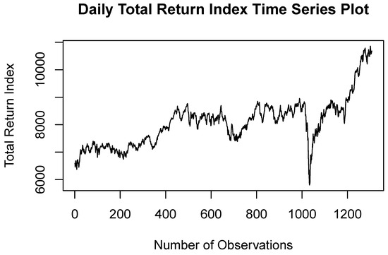
Figure 1.
Time series plot of the total return index of the ALSTRI from 1 February 2016 to 26 April 2021.
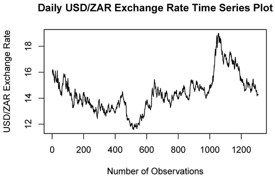
Figure 2.
Time series plot of the USD–ZAR exchange rate from 1 February 2016 to 26 April 2021.
On 5 March 2020, the National Institute for Communicable Diseases (NIDC) of South Africa reported the first case of COVID-19 in South Africa (NICD n.d.). As a result, the financial markets experienced a market shock. There was a decline in the ALSTRI on 19 March 2020. A nationwide lockdown was announced to commence on 26 March 2020. Thus, there was a steep decline in the ALSTRI during March 2020 as a result of the COVID-19 pandemic, whereas the USD–ZAR exchange rate was significantly high during March 2020 and was at its peak in April 2022 after the first reported COVID-19 case and the first national lockdown in South Africa. Figure 3 and Figure 4 illustrate the log returns of the ALSTRI and USD–ZAR exchange rate, respectively. The log returns were computed in order to stabilise the variance. The log returns data in Figure 3 and Figure 4 are centred around zero, which implies that the variance is stabilised and the data are stationary. The instability of the markets with a day-to-day change in prices exemplified positive spikes showing daily gains, and negative spikes showing daily losses. There were significant losses of the ALSTRI during March 2020 after the first reported COVID-19 case and the first national lockdown in South Africa, whereas the ZAR was significantly high during March 2020 and was at its peak in April 2022 after the first reported COVID-19 case and the first national lockdown in South Africa.
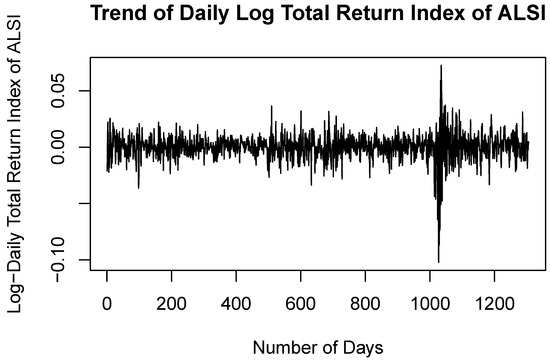
Figure 3.
Time series plot of log-returns for the ALSTRI from 1 February 2016 to 26 April 2021.
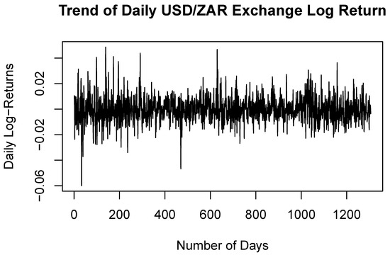
Figure 4.
Log-returns plot of the USD–ZAR exchange rate from 1 February 2016 to 26 April 2021.
Table 1 illustrates the summary statistics of the ALSTRI and USD–ZAR exchange rate daily data from 1 February 2016 to 26 April 2021. The results in Table 1 indicate that the ALSTRI ranges from 5802 recorded on 19 March 2020 to 10,860 recorded on 16 April 2021. In accordance with Table 1, the minimum and maximum indices are far from the mean, which demonstrates the presence of extreme events such as the COVID-19 pandemic. The mean is lower than the median and the skewness of the log returns is negative; this shows that the presence of extreme values lies more in the left tail. The kurtosis value of 4.175, which is greater than 3, demonstrates that the distribution of the returns is leptokurtic and fat-tailed. The lowest exchange rate was R11.58, recorded on 23 February 2018, and the highest exchange rate was R18.99, recorded on 23 April 2020, during the second month following the initial reported COVID-19 cases in South Africa. The minimum and maximum USD–ZAR exchange rates of R11.58 and R18.99, respectively, are far from the mean, which confirms the presence of extreme events. The mean is greater than the median and the skewness of the log returns is positive; this indicates the existence of extreme values in the right tail. The kurtosis value of 0.719 is less than 3, suggesting that the distribution of the exchange rate is platykurtic.

Table 1.
Descriptive statistics of the ALSTRI and USD–ZAR exchange rate.
4.2. EVT Results
This sub-section presents the EVT models, namely the GEVD, bGEVD, GEVD, GPD, and Poisson point process. The extreme values are fitted at the tails of the data. The block maxima approach as well as the POT approach were employed in the study. The monthly block maxima approach was used to model the ALSTRI and the USD–ZAR exchange rate. The MLE and the Bayesian parameter estimation methods were used to estimate the location (), scale (), and shape () parameters.
4.3. GEVD Models
The MLE parameter estimates for the GEVD monthly maxima of the ALSTRI and the USD–ZAR exchange rate are presented in Table 2. The estimate of the shape parameter is negative and the confidence intervals at of the shape parameter do not include zero, which implies that the data can be modelled by the Weibull family of distributions because .

Table 2.
MLE parameter estimates and standard errors (in parentheses) for the GEVD monthly maxima.
Makatjane and Moroke (2021) conducted a study titled “Predicting Extreme Daily Regime Shifts in Financial Time Series Exchange/Johannesburg stock exchange-all share index”. The Bayesian Markov chain Monte Carlo (MCMC) parameter estimation approach was employed to estimate the parameters for the GEVD. According to Makatjane and Moroke (2021), complex likelihood functions with higher dimensions are difficult to estimate; thus, the Bayesian methods have densities to solve complex model estimation. The shape parameter was found to be negative, suggesting that FTSE/JSE-ALSI returns conform to a Weibull class of distribution. The Bayesian parameter estimates for the GEVD monthly maxima of the ALSTRI and the USD–ZAR exchange rate are presented in Table 3. The estimate of the shape parameter is positive and the confidence intervals at of the shape parameter do not include zero, which implies that the data can be modelled by the Frèchet family of distributions.

Table 3.
Bayesian parameter estimates for the GEVD monthly maxima.
Diagnostic Plots
The diagnostic plot for assessing the GEVD monthly maxima are displayed in Figure 5 and Figure 6, respectively. The P-P plot, Q-Q plot, return level, and density plot assess whether the dataset follows the GEVD. The ALSTRI and the USD–ZAR exchange rate are plotted on the theoretical distribution, which indicates that the plotted points are linear, implying that the GEVD is a good fit for the financial market data. The return level plot shows the return period against the return level together with an estimated 95% confidence interval.
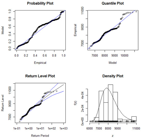
Figure 5.
GEVD monthly maxima diagnostic plots for the all-share total return index.
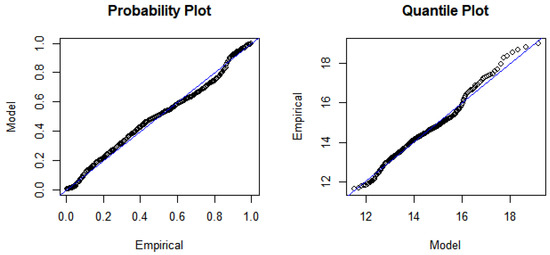
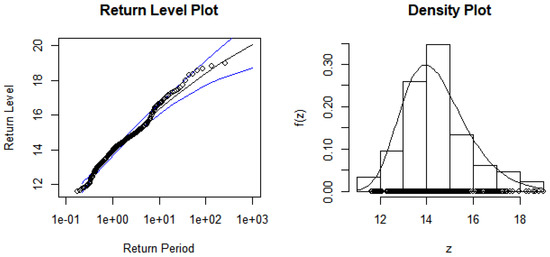
Figure 6.
GEVD monthly maxima diagnostic plots for the USD–ZAR exchange rate.
4.4. bGEVD Models
In accordance with Vandeskog et al. (2022), the bGEVD is only applicable for modelling heavy-tailed or exponential phenomena where > 0. No studies have been conducted on bGEVD in the field of finance or financial markets. However, there have been limited studies conducted on bGEVD in other fields of application (Vandeskog et al. 2021a, 2021b, 2022; Castro-Camilo 2021) In a study conducted by Vandeskog et al. (2021a), block maxima were used to model the data using bGEVD, whereas Vandeskog et al. (2022) modelled the yearly maxima of the sub-daily precipitation using bGEVD. The monthly maxima of the ALSTRI and the USD–ZAR exchange rate were used to model the bGEVD. Prior to modelling the JSE financial market data with the bGEVD model, the explanatory variables were standardised to have a mean of zero and a standard deviation of 1 (Vandeskog et al. 2021b). Thus, Figure 7 and Figure 8 display the standardised monthly maxima of the ALSTRI and the USD–ZAR exchange rate used in modelling the bGEVD model.
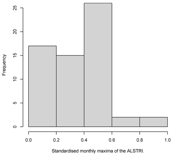
Figure 7.
Histogram displaying the standardised monthly maxima of the ALSTRI.
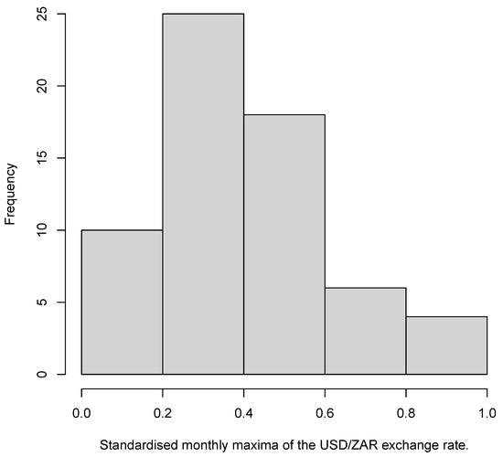
Figure 8.
Histogram displaying the standardised monthly maxima of the USD–ZAR exchange rate.
Statistically, the location-spread parameterisation predominates when compared to the mean and standard deviation of the distribution (Rue et al. 2009). Castro-Camilo (2021) assert that the new parameterisation allows for the interpretation of the location and spread parameters even when the mean and the variance are unknown. The results of the bGEVD for the ALSTRI and the USD–ZAR exchange rate monthly maxima are presented in Table 4. The R-INLA package was used to model the bGEVD.

Table 4.
Posterior means, standard deviation (SD ()), and quantiles for the estimated linear regression coefficients , and , and hyperparameters of the bGEVD INLA fits for the monthly maxima of the JSE financial market data.
Table 4 displays the bGEVD intercept, explanatory variables, which are the monthly maxima of the ALSTRI, and the USD–ZAR exchange rate, as well as the regression coefficients and . There is a positive linear trend term indicating an increase in the ALSTRI and the USD–ZAR exchange rate over time. The explanatory variables have a greater effect on the location parameter. Thus, an increase in the ALSTRI and the USD–ZAR exchange rate is expected with more variance in the distribution of the extremes.
4.5. GEVD Models
The r-largest-order statistics was employed with the aim to model the characterisation behaviour of extremes of the JSE financial data, rather than making use of a single maximum value within a block. The r-largest-order approach is usually used in cases where there are limited data. The monthly block maxima approach was employed to model the five-year daily data. In the case where , it is similar to the results of the GEVD, implying that the values are sampled from the monthly block maxima. The MLE and Bayesian parameter estimation methods were employed to fit the parameters of the GEVD. The MLE estimated parameters are location (), scale (), shape (), the confidence interval of the shape parameter, and the negative log-likelihood ().
The MLE parameter estimation approach was employed by various authors on GEVD (Kajambeu et al. 2020; Nemukula and Sigauke 2018). Table 5 presents the GEVD model parameter estimates for the location (), scale (), and shape () using the MLE parameter estimation technique for . The estimates of shape parameters of of the USD–ZAR exchange rate are all negative and the confidence intervals at of the shape parameters do not include zero, which implies that the data can be modelled by the Weibull family of distributions because . Table 5 shows that the estimates of shape parameters of of the ALSTRI are all negative and the confidence intervals at of the shape parameters for ,…, do not include zero, which implies that the data can be modelled by the Weibull family of distributions because .

Table 5.
MLE parameter estimates and standard errors (in parantheses) for the GEVD monthly maxima.
The study by Santos da Silva and Ferraz do Nascimento (2019) applied the Bayesian MCMC approach to model the GEVD for r = 1, … , r = 10. The results revealed that the Bayesian method produced more accurate estimates as compared to other parameter estimation approaches such as the MLE. The MCMC Bayesian parameter estimation method was employed by e Silva et al. (2020) to model the r-largest-order statistics of the environmental and financial data. As r increased, estimator accuracy improved. Table 6 presents the Bayesian parameter estimates for the ALSTRI and the USD–ZAR exchange rate. For both types of financial market data, the estimates of shape parameters for are positive and the confidence intervals at of the shape parameter do not include zero, which implies that the data can be modelled by the Frèchet family of distributions. In accordance with Nemukula and Sigauke (2018); Tawn (1988), the high values of r are likely to violate the model and lead to the occurrence of bias, whereas too low values of r can lead to a high variance of the estimator; thus, r must be as small as possible. The results of Nemukula and Sigauke (2018) revealed that was the best fit for the data. Kajambeu et al. (2020) found that the suitable-fit order statistics for the data was .

Table 6.
Bayesian MCMC parameter estimates for GEVD monthly maxima with r = 1, … , r = 10, posterior means and confidence intervals of the shape parameter with lower limit (2.5%) and upper limit (97.5%).
According to Table 5 and Table 6, the shape parameter decreases as r increases. In conclusion, the suitable model for the ALSTRI was found to be GEVD, and for the USD–ZAR exchange rate, the best model is GEVD, that is, for the present study.
4.5.1. Entropy Difference Test Results
Testing the GEVD goodness-of-fit using a sequence of the null hypotheses is fundamental (Nemukula and Sigauke 2018).The entropy difference test is used in this study to test if the null hypothesis : the GEVD fits the sample of the r-largest-order statistics well for ,…, R, where R is the maximum of the specified number of the top-order statistics test (Nemukula and Sigauke 2018).
Table 7 presents the entropy difference test results. The forward and the strong stop are also provided.

Table 7.
Entropy difference test for the GEVD monthly maxima.
4.5.2. Diagnostic Plots
The diagnostic plots for assessing the GEVD model for the ALSTRI and the USD–ZAR exchange rate are displayed in Figure 9 and Figure 10, respectively. The P-P plot, Q-Q plot, return level, and density plot are displayed.
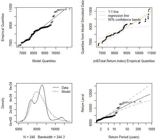
Figure 9.
GEVD diagnostic plots of the ALSTRI.
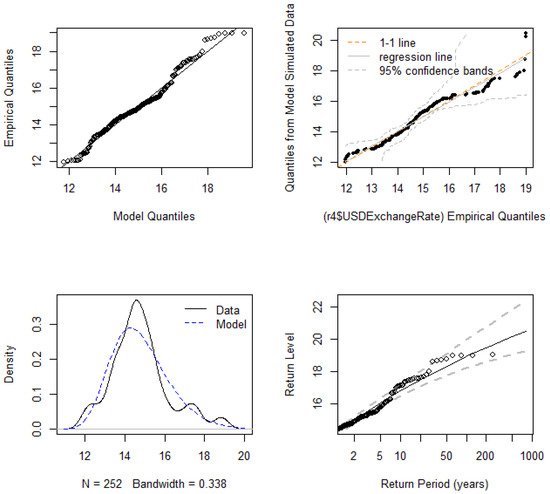
Figure 10.
GEVD diagnostic plots of the USD–ZAR exchange rate.
4.6. GPD Models
This sub-section presents the results of the analysis of the GPD. The POT method was employed to fit the GPD model. To fit the GPD model, a subjective choice of a suitable threshold value should be obtained. In order to select the suitable thresholds for the JSE financial data, the mean excess plot and the threshold stability plot were used. Zeng et al. (2022) fitted POT to the daily average return of the Shanghai stock market in different periods. The results of the study indicated that the POT model was found to be an effective fit for the thick tail distribution of the Shanghai stock market. Thus, it was concluded that the POT method is an effective method to measure extreme risk. Figure 11 and Figure 12 display the mean residual life plots of the ALSTRI and the USD–ZAR exchange rate, respectively. The mean residual life of the ALSTRI and the USD–ZAR exchange rate in Figure 11 and Figure 12 display the average excess values over given thresholds for a series of thresholds. In order to model and select a valid GDP model, the mean residual life plot should be approximately linear above the threshold (Coles et al. 2001).
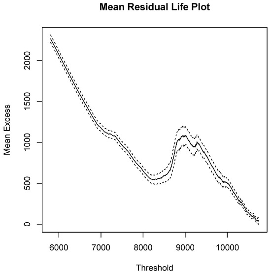
Figure 11.
Mean residual life plot for ALSTRI.
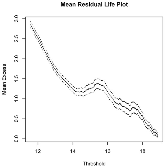
Figure 12.
Mean residual life plot for the USD–ZAR exchange rate.
The mean residual life plot of the ALSTRI in Figure 11 shows evidence of linearity above u = 8500 and Figure 12 provides evidence that the USD–ZAR exchange rate is approximately linear above u = 14.25. Table 8 displays the findings of the GPD parameter estimates of the ALSTRI and the USD–ZAR exchange rate. The shape parameter for the ALSTRI is positive () and the confidence intervals are significantly different from zero. This implies that the ALSTRI is equivalent to the Pareto distribution. The shape parameter for the USD–ZAR exchange rate is negative () and the confidence intervals contain zero. This means the ALSTRI has a light tail as compared to the exponential distribution. Thus, the tail of the USD–ZAR exchange rate is equivalent to the exponential distribution.

Table 8.
MLE parameter estimates and standard errors (in parentheses) for the GPD Model.
4.7. Poisson Point Process Models
In accordance with Coles et al. (2001), the Poisson point process method is similar to the GPD approach; this implies that the mean residual life plot of the ALSTRI and the USD–ZAR exchange rate are the same for the Poisson point process as those of the GPD.
Figure 11 and Figure 12 show the mean residual plots for the financial market data. Similarly to the GPD outcomes, the mean residual life plot of the ALSTRI in Figure 11 provides evidence of linearity above u = 8500 and Figure 12 provides evidence that the USD–ZAR exchange rate is approximately linear above u = 14.25 for the Poisson point process. The threshold stability plot of the ALSTRI and the USD–ZAR exchange rate are presented in Figure 13 and Figure 14, respectively. The parameter estimates are presented in Table 9.
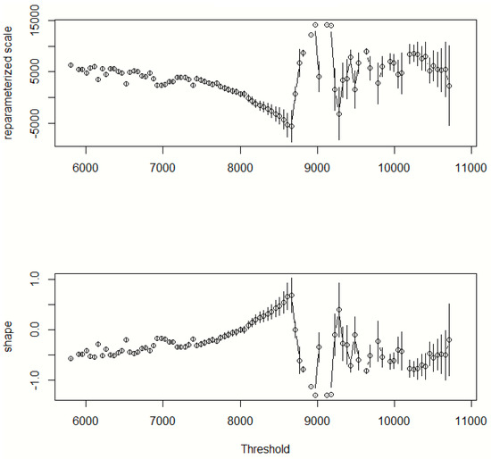
Figure 13.
Threshold stability plot for ALSTRI.
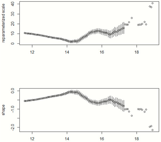
Figure 14.
Threshold stability plot for USD–ZAR exchange rate.

Table 9.
Parameter estimates and standard errors (in parentheses) for the Poisson point process.
Table 9 displays the results of the Poisson point process parameter estimates of the ALSTRI and the USD–ZAR exchange rate. The shape parameter of the ALSTRI is positive () and the confidence intervals are significantly different from zero. This implies that the ALSTRI can be modelled according to the Pareto family of distribution, whereas the shape parameter of the USD–ZAR exchange rate is negative () and the confidence intervals contains zero. This means that the USD–ZAR exchange rate data can be fitted by the exponential family of distributions.
4.8. Return Levels
Table 10 displays the return levels and corresponding return periods of the EVT models, namely GEVD, bGEVD, GEVD, GPD, and the Poisson point process. There is an increase in return levels as the return period rises. Return levels together with the corresponding return periods for 5 years, 10 years, 20 years, 50 years, and 100 years were computed.

Table 10.
Monthly block maxima return levels for GEVD, bGEVD, GEVD, GPD, and the Poisson point process.
The 100-year return levels of the GEVD and bGEVD are slightly equivalent to the maximum observed values for both the ASTRI and the USD–ZAR exchange rate, respectively. Thus, the monthly block maxima return levels reveal that the ALSTRI and the USD–ZAR exchange rate will exceed 10,860 and R18.99, respectively. In conclusion, the findings of the return levels for the bGEVD and GEVD models suggest that the two models result in similar return level outcomes. This suggests that bGEVD can be a suitable alternative for the GEVD for modelling block maxima (Castro-Camilo 2021; Vandeskog et al. 2021a). The return level results for the GEVD model suggest that the ALSTRI will exceed 10,796.5 at least once in 100 years, while the USD–ZAR exchange rate will surpass R18.87 at least once in 100 years. The GEVD return levels are closely comparable with the GEVD and bGEVD monthly block maxima estimates. According to Coles et al. (2001), the threshold approach is more efficient than the block maxima method and POT is a better alternative to the block maxima or block minima approach due to its capability to use as much as possible of the available information. In accordance with the findings of Table 10, the return levels of the GPD suggest that the ALSTRI will exceed 19,092.42 at least once in 100 years, while the USD–ZAR exchange rate will surpass R23.72 at least once in 100 years. Thus, the financial markets will exceed the maximum observations in the future. These findings further reveal that the GPD return level estimates are much higher than the GEVD, bGEVD, and GEVD return levels. According to the results for the Poisson point process return levels, the 100-year return level of the ALSTRI exceeds the maximum. This implies that the ALSTRI is likely to exceed the observed maximum total returns. With regards to the USD–ZAR exchange rate, the 100-year return levels of the exchange rate exceed the maximum of R18.99. This suggests that the maximum exchange rate is likely to be exceeded at least once in 100 years. In actual fact, the ALSTRI and USD–ZAR exchange rate will surpass 17,501.63 and R23.72, respectively, at least once in 100 years. The Poisson point process return level estimates are quite comparable with the GPD estimates.
Overall, the findings in this study reveal that the block maxima return level estimates are comparable regardless of the block maxima technique used. Likewise, the POT return level estimates are also comparable, and are much higher than the block maxima return level estimates. The block maxima return level estimates, however, are closer to the reality than the POT estimates in this study. It was also found that the bGEVD cuts off to the maximum observed value at the 50-year return period for both the ALSTRI and USD–ZAR exchange rate.
5. Conclusions and Recommendations
The main purpose of this study was to model the extreme behavious of the Johannesburg stock exchange (JSE) financial market data and compare the block maxima approach and the POT approach in terms of their ability in modelling the financial market data. The volatility of the markets and day-to-day fluctuation in prices were highlighted by positive spikes displaying daily profits and negative spikes showing daily losses in the study. The first recorded COVID-19 case and the first national lockdown in South Africa caused the USD–ZAR exchange rate to spike in March 2020 and reach its peak in April 2022, and there were significant losses of the ALSTRI during March 2020. The data for both the ALSTRI and USD–ZAR exchange rate stabilised after the log transformation and became stationary.
In conclusion, based on the GEVD findings, it will be expected that South Africa will experience an extreme increase in the USD–ZAR exchange rate. There will not be any unexpectedly high total returns for the ALSTRI, due to the fact that the 100-year return of the ALSTRI monthly maxima is roughly comparable to the maximum observation. The GEVD return levels reveal that the ALSTRI and USD–ZAR exchange rate will exceed 11,100.08 and R19.23, respectively, at least once in 100 years. The monthly maxima data were used in modelling the ALSTRI and the USD–ZAR exchange rate using the bGEVD method, which is an alternative to the GEVD technique. The bGEVD smoothly incorporates the left tail of a Gumbel distribution and the right tail of a Fréchet distribution. The results reveal that there is a positive linear trend term indicating an increase in the ALSTRI and the USD–ZAR exchange rate over time. The explanatory variables have a greater effect on the location parameter. The 100-year return levels are slightly equivalent to the maximum observed values for both the ALSTRI and the USD–ZAR exchange rate. Thus, the bGEVD return levels reveal that the ALSTRI and the USD–ZAR exchange rate will exceed 10,860 and R18.99, respectively. In conclusion, the findings of the return levels for the bGEVD and GEVD models suggest that the two models result in similar outcomes. This implies that bGEVD can be a feasible alternative to the GEVD for modelling block maxima. The 100-year return levels of the monthly GEVD, bGEVD, and GEVD models are almost equal to the maximum observations of the financial markets, while the 100-year return levels for the GPD and the Poisson point process models were very much higher than the maximum observations of the financial market data. The Poisson point process return level estimates are quite comparable with the GPD estimates. In actual fact, the ALSTRI and USD–ZAR exchange rate will surpass 17,501.63 and R23.72, respectively, at least once in 100 years. Overall, the findings in this study suggest that investors will experience higher gains in the total returns of the ALSI. The USD–ZAR exchange rate return levels suggest that the ZAR will become more unstable in the long run. As the ZAR goes higher it will affect the inflation and the economy of South Africa. The USD will become much stronger, and this will affect the ZAR as the USD appreciates or strengthens, which will depreciate or weaken the South African currency.
In conclusion, both the block maxima and POT approaches have revealed long-run increases in the ALSTRI and USD–ZAR exchange rate. One of the major findings of this study is that the return level estimates of the block maxima and POT approaches are not comparable for the JSE financial market data, although both approaches can be used to predict future volatility in the financial markets. The study further revealed that the bGEVD is more suitable for relatively short-term forecasting since it cuts off at the 50-year return level.
5.1. Recommendations
There are rare events that contribute towards the negative impact on the financial markets, such as pandemics and financial crises. Due to the instability and unpredictability of the financial markets, the manifestation of the financial crises and pandemics can put investors, financial economists, and risk experts in an uneasy situation, not knowing whether the investments will return gains or losses, as well as not knowing the impact of these rare events on the stock and financial markets. Financial market volatility can result in risk, whether big or small, that can be concealed in the tails rather than the mean. Therefore, it is recommended that risk management systems consider cutting-edge techniques such as advanced EVT methods, which comprise, among others, the Poisson point process, r-largest-order statistics, and bGEVD for anticipating the uncommon extreme occurrences with significant ramifications that could be harmful to the financial industry. Financial disasters can be mitigated by using the advanced EVT techniques to identify and examine the characteristics of extreme value behaviour and thereby prevent the risk. The insufficient amount of data available for model estimation is an inherent challenge in any extreme value investigation. Since extremes are by definition rare, the model estimates, particularly those of extreme return levels, have a high degree of variance. Instead of focusing merely on the traditional methods of block maxima, the use of advanced extreme value methods that accommodates even small datasets such as r-largest-order statistics, bGEVD, and the Poisson point process is encouraged. The use of statistical methods that can predict the occurrence of extremes, focusing on the tails of the distribution to predict the future events, is recommended.
5.2. Future Studies
The researchers discovered that there are no studies conducted on bGEVD in the field of finance or financial markets. In the future, more studies on bGEVD, vine copulas, and r-largest-order bGEVD can be conducted in the financial markets and/or finance sector. The frequency of the occurrence of extreme returns in the financial sector can be studied to assist in enhancing risk management systems.
Author Contributions
Conceptualization, M.K.M. and D.M.; methodology, D.M.; software, M.K.M.; validation, M.K.M. and D.M.; formal analysis, M.K.M. and D.M.; investigation, M.K.M. and D.M.; resources, M.K.M. and D.M.; data curation, M.K.M. and D.M.; writing–original draft preparation, M.K.M. and D.M.; writing–review and editing, M.K.M. and D.M.; visualization, M.K.M. and D.M.; supervision, D.M.; project administration, M.K.M. and D.M.; funding acquisition, D.M. All authors have read and agreed to the published version of the manuscript.
Funding
The APC was funded by the University of Limpopo as the institution of affiliation of the author.
Informed Consent Statement
Not applicable since the study does not involving humans.
Data Availability Statement
The data supporting this study is available from the Johannesburg Stock Exchange (JSE) upon request and more data from JSE can be accessed for a certain amount of fee.
Acknowledgments
The authors would like to thank the Johannesburg Stock Exchange (JSE) for providing the data used in this study, and the University of Limpopo for supporting the publication of this study.
Conflicts of Interest
The authors declare no conflict of interest. The funders had no role in the design of the study, in the writing of the manuscript, or in the decision to publish the results.
Abbreviations
The following abbreviations are used in this manuscript:
| ALSTRI | All-Share Total Return Index |
| bGEVD | Blended Generalised Extreme Value Distribution |
| COVID-19 | Coronavirus of 2019 |
| EVT | Extreme Value Theory |
| FTSE/JSE-ALSI | Financial Time Series Exchange/Johannesburg Stock Exchange–All-Share index |
| GEVD | Generalised Extreme Value Distribution |
| GEVD | r-largest Generalised Extreme Value Distribution |
| GPD | Generalised Pareto Distribution |
| i.i.d | independent and identically distributed |
| INLA | Integrated Nested Laplace Approximation |
| JSE | Johannesburg Stock Exchange |
| MCMC | Markov Chain Monte Carlo |
| MLE | Maximum Likelihood Estimation |
| NICD | National Institute for Communicable Diseases |
| POT | Peak-Over-Threshold |
| P-P plot | Probability–Probability plot |
| p-value | Probability Value |
| Q-Q plot | Quantile–Quantile plot |
| SAWS | South African Weather Services |
| USD–ZAR | United States Dollar against the South African Rand |
| ZAR | South African Rand |
References
- Afuecheta, Emmanuel, Chigozie Utazi, Edmore Ranganai, and Chibuzor Nnanatu. 2023. An Application of extreme value theory for measuring Financial Risk in BRICS Economies. Annals of Data Science 10: 251–90. [Google Scholar] [CrossRef]
- Andreev, Vladimir O., Sergey E. Tinykov, Oksana P. Ovchinnikova, and Gennady P. Parahin. 2012. Extreme value theory and peaks over threshold model in the Russian Stock Market. Journal of the Siberian Federal University. Series: Technique and Technology 5: 111–21. [Google Scholar]
- Bordo, Michael D., and John S. Landon-Lane. 2010. The Global Financial Crisis of 2007–2008: Is It Unprecedented? (No. w16589). Cambridge: National Bureau of Economic Research. [Google Scholar]
- Castro-Camilo, Daniela, Raphaël Huser, and Håvard Rue. 2021. Practical strategies for GEV-based regression models for extremes. arXiv arXiv:2106.13110. [Google Scholar]
- Chikobvu, Delson, and Owen Jakata. 2020. Analysing extreme risk in the South African Financial Index (J580) using the generalised extreme value distribution. Statistics, Optimization & Information Computing 8: 915–33. [Google Scholar]
- Coles, Stuart, Joanna Bawa, Lesley Trenner, and Pat Dorazio. 2001. An Introduction to Statistical Modeling of Extreme Values. London: Springer, vol. 208, p. 208. [Google Scholar]
- Darškuvienė, Valdonė. 2010. Financial Markets: Study Guide. Kaunas: Vytautas Magnus University. [Google Scholar]
- e Silva, Wyara Vanesa Moura, Fernando Ferraz do Nascimento, and Marcelo Bourguignon. 2020. A change-point model for the r-largest-order statistics with applications to environmental and financial data. Applied Mathematical Modelling 82: 666–79. [Google Scholar] [CrossRef]
- Ferreira, Ana, and Laurens De Haan. 2015. On the Block Maxima Method in Extreme Value Theory: PWM Estimators. Available online: https://www.jstor.org/stable/43556515 (accessed on 27 September 2023).
- Gencay, Ramazan, and Faruk Selçuk. 2004. Extreme value theory and Value-at-Risk: Relative performance in emerging markets. International Journal of Forecasting 20: 287–303. [Google Scholar] [CrossRef]
- Gilli, Manfred, and Evis Këllezi. 2006. An application of extreme value theory for measuring financial risk. Computational Economics 27: 207–28. [Google Scholar] [CrossRef]
- Gnedenko, Boris. 1943. Sur la Distribution Limite du Terme Maximum d’une Serie Aleatoire. Annals of Mathematics. pp. 423–53. Available online: https://www.jstor.org/stable/1968974 (accessed on 5 October 2023).
- Iyke, Bernard Njindan, and Sin-Yu Ho. 2021. Exchange rate exposure in the South African stock market before and during the COVID-19 pandemic. Finance Research Letters 43: 102000. [Google Scholar] [CrossRef]
- Jakata, Owen, and Delson Chikobvu. 2022. Extreme Value Modelling of the Monthly South African Industrial Index (J520) Returns. Statistics, Optimization & Information Computing 10: 383–400. [Google Scholar]
- JSE Limited. 2023. History of the JSE [Online]. Available online: http://www.jse.co.za/About-Us/History-Of-The-JSE.aspx (accessed on 27 June 2023).
- Kajambeu, Robert, Caston Sigauke, Alphonce Bere, Delson Chikobvu, Daniel Maposa, and Murendeni Maurel. 2020. Probabilistic Flood Height Estimation of the Limpopo River at the Beitbridge using r-Largest Order Statistics. Applied Mathematics 14: 191–204. [Google Scholar]
- Karmakar, Madhusudan, and Girja K. Shukla. 2015. Managing extreme risk in some major stock markets: An extreme value approach. International Review of Economics & Finance 35: 1–25. [Google Scholar]
- Longin, François, and Giovanni Pagliardi. 2016. Tail relation between return and volume in the US stock market: An analysis based on extreme value theory. Economics Letters 145: 252–54. [Google Scholar] [CrossRef]
- Makatjane, Katleho, and Ntebogang Moroke. 2021. Predicting Extreme Daily Regime Shifts in Financial Time Series Exchange/Johannesburg Stock Exchange—All Share Index. International Journal of Financial Studies 9: 18. [Google Scholar] [CrossRef]
- Makatjane, Katleho, Ntebo Moroke, and Elias Munapo. 2021. Predicting the Tail Behavior of Financial Times Stock Exchange/Johannesburg Stock Exchange (FTSE/JSE) Closing Banking Indices: Extreme Value Theory Approach. In Handbook of Research on Emerging Theories, Models, and Applications of Financial Econometrics. Cham: Springer, pp. 31–64. [Google Scholar]
- Makhwiting, Monnye Rhoda, Caston Sigauke, and Maseka Lesaoana. 2014. Modelling tail behavior of returns using the generalized extreme value distribution. Economics, Management and Financial Markets 9: 41. [Google Scholar]
- Maposa, Daniel, Anna M. Seimela, Caston Sigauke, and James J. Cochran. 2021. Modelling temperature extremes in the Limpopo province: Bivariate time-varying threshold excess approach. Natural Hazards 107: 2227–46. [Google Scholar] [CrossRef]
- McNeil, Alexander J., and Rüdiger Frey. 2000. Estimation of tail-related risk measures for heteroscedastic financial time series: An extreme value approach. Journal of Empirical Finance 7: 271–300. [Google Scholar] [CrossRef]
- Nemukula, Murendeni M., and Caston Sigauke. 2018. Modelling average maximum daily temperature using r largest order statistics: An application to South African data. Jàmbá: Journal of Disaster Risk Studies 10: 1–11. [Google Scholar] [CrossRef]
- NICD: Communiqué. n.d. Available online: https://www.nicd.ac.za/first-case-of-covid-19-coronavirus-reported-in-sa/ (accessed on 15 July 2021).
- Qian, Lingling, Yuexiang Jiang, and Huaigang Long. 2023. Extreme risk spillovers between China and major international stock markets. Modern Finance 1: 30–34. [Google Scholar] [CrossRef]
- Rocco, Marco. 2014. Extreme value theory in finance: A survey. Journal of Economic Surveys 28: 82–108. [Google Scholar] [CrossRef]
- Rue, Håvard, Sara Martino, and Nicolas Chopin. 2009. Approximate Bayesian inference for latent Gaussian models by using integrated nested Laplace approximations. Journal of the Royal Statistical Society: Series B (Statistical Methodology) 71: 319–92. [Google Scholar] [CrossRef]
- Rydman, Max. 2018. Application of the Peaks-Over-Threshold Method on Insurance Data. Uppsala: Department of Mathematics, Uppsala University. [Google Scholar]
- Santos da Silva, Renato, and Fernando Ferraz do Nascimento. 2019. Extreme Value Theory Applied to r Largest Order Statistics under the Bayesian Approach. Revista Colombiana de Estadística 42: 143–66. [Google Scholar] [CrossRef]
- Sikhwari, Thendo, Nthaduleni Nethengwe, Caston Sigauke, and Hector Chikoore. 2022. Modelling of extremely high rainfall in Limpopo Province of South Africa. Climate 10: 33. [Google Scholar] [CrossRef]
- Su, Xianfang. 2020. Measuring extreme risk spillovers across international stock markets: A quantile variance decomposition analysis. The North American Journal of Economics and Finance 51: 101098. [Google Scholar] [CrossRef]
- Szczygielski, Jan Jakub, and Chimwemwe Chipeta. 2023. Properties of returns and variance and the implications for time series modelling: Evidence from South Africa. Modern Finance 1: 35–55. [Google Scholar] [CrossRef]
- Takyi, Paul Owusu, and Isaac Bentum-Ennin. 2021. The impact of COVID-19 on stock market performance in Africa: A Bayesian structural time series approach. Journal of Economics and Business 115: 105968. [Google Scholar] [CrossRef]
- Tawn, Jonathan A. 1988. An extreme-value theory model for dependent observations. Journal of Hydrology 101: 227–50. [Google Scholar] [CrossRef]
- Van der Merwe, Sean, Darren Steven, and Martinette Pretorius. 2018. Bayesian extreme value analysis of stock exchange data. arXiv arXiv:1804.01807. [Google Scholar]
- Vandeskog, Silius M., Sara Martino, and Daniela Castro-Camilo. 2021a. Modelling block maxima with the blended generalised extreme value distribution. Paper presented at the 22nd European Young Statisticians Meeting, Ljubljana, Slovenia, Sepember 6–10; vol. 138. [Google Scholar]
- Vandeskog, Silius M., Sara Martino, Daniela Castro-Camilo, and Haavard Rue. 2021b. Modelling Short-Term Precipitation Extremes with the Blended Generalised Extreme Value Distribution. Available online: https://repository.kaust.edu.sa/handle/10754/669211.1 (accessed on 27 September 2023).
- Vandeskog, Silius M., Sara Martino, Daniela Castro-Camilo, and Håvard Rue. 2022. Modelling sub-daily precipitation extremes with the blended generalised extreme value distribution. Journal of Agricultural, Biological and Environmental Statistics 27: 598–621. [Google Scholar] [CrossRef]
- Wei, Xiaoyun, and Liyan Han. 2021. The impact of COVID-19 pandemic on transmission of monetary policy to financial markets. International Review of Financial Analysis 7: 101705. [Google Scholar] [CrossRef]
- Zeng, Xiaohua, Changzhou Liang, and Chiping Yuan. 2022. An empirical study on extreme risk of Chinese stock market based on POT model. Paper presented at 2022 3rd International Conference on Internet and E-Business, Madrid, Spain, June 15–17; pp. 89–93. [Google Scholar]
- Zhang, Wenting, and Shigeyuki Hamori. 2021. Crude oil market and stock markets during the COVID-19 pandemic: Evidence from the US, Japan, and Germany. International Review of Financial Analysis 74: 101702. [Google Scholar] [CrossRef]
Disclaimer/Publisher’s Note: The statements, opinions and data contained in all publications are solely those of the individual author(s) and contributor(s) and not of MDPI and/or the editor(s). MDPI and/or the editor(s) disclaim responsibility for any injury to people or property resulting from any ideas, methods, instructions or products referred to in the content. |
© 2023 by the authors. Licensee MDPI, Basel, Switzerland. This article is an open access article distributed under the terms and conditions of the Creative Commons Attribution (CC BY) license (https://creativecommons.org/licenses/by/4.0/).