Large-Scale Portfolio Optimization Using Biogeography-Based Optimization

Abstract

Portfolio optimization is a mathematical formulation whose objective is to maximize returns while minimizing risks. A great deal of improvement in portfolio optimization models has been made, including the addition of practical constraints. As the number of shares traded grows, the problem becomes dimensionally very large. In this paper, we propose the usage of modified biogeography-based optimization to solve the large-scale constrained portfolio optimization. The results indicate the effectiveness of the method used.

1. Introduction

A portfolio can be defined as a collection of assets, which can include cash, real estate, stocks, or crypto. Portfolio optimization concerns maximizing returns and minimizing risks; returns are the expected profit from the investment, whereas risks are the possible changes in values of the investment. In Markowitz (1952), the authors proposed the use of the means and variances of the portfolio as the return and risk measures. Good practice in portfolio optimization is very crucial in investment, because it greatly affects the outcome of the investment. In this paper, we focus on portfolios consisting of correlated stocks.

The model proposed by Markowitz (1952) has been studied by many researchers over the years. A possible approach for the problem is the capital asset pricing model (CAPM). CAPM has been used extensively by many financial practitioners. In Parmikanti et al. (2020), the authors studied portfolio optimization under CAPM with a heteroscedastic model for the return series. Since its introduction, many improvements have been made to the model. Some improvements add practical constraints, which can be discrete or continuous; hence, the resulting model becomes mixed-integer nonlinear programming (MINLP). For instance, Jobst et al. (2001) and Bartholomew-Biggs and Kane (2009) considered adding roundlot constraints, which means that shares must be bought in a multiple of some integer. In Jobst et al. (2001), the authors used the FortMP solver, whereas Bartholomew-Biggs and Kane (2009) used DIRECT hybridized with quasi-Newton methodology. In Jobst et al. (2001), the authors also noted that the resulting efficiency is not continuous, making CAPM inapplicable in this case. With increasing complexity, various techniques also emerged. AUGMECON2 is a state-of-the-art multi-objective MINLP solver. It was introduced by Mavrotas and Florios (2013) and has been shown to very effective in solving multi-objective MINLP. Recent use of AUGMECON2 in portfolio optimization can be found in Chen et al. (2021). The downside of this method is its computational complexity. In Chen et al. (2021), the authors noted that for some large-dimensional problems, AUGMECON2 did not give a converged solution after 7 days.

To circumvent the complexity of exact methods, an efficient optimizer is needed. One popular approach is to use metaheuristic algorithms. Metaheuristic algorithms are usually inspired by natural processes in biology, chemistry, physics, or society. Most of the time, it is expected that metaheuristic algorithms can produce near-optimal solutions. Furthermore, an exact method is expected to be implemented later to obtain more accuracy, such in Bartholomew-Biggs and Kane (2009). In Chang et al. (2000), the authors proposed a series of modified metaheuristic algorithms that exploit the structure of the MV model with cardinality and quantity constraints. The metaheuristic algorithms used were genetic algorithm (GA), tabu search (TS), and simulated annealing (SA). To handle the cardinality and quantity constraints, they implemented an algorithm to adjust the solutions.

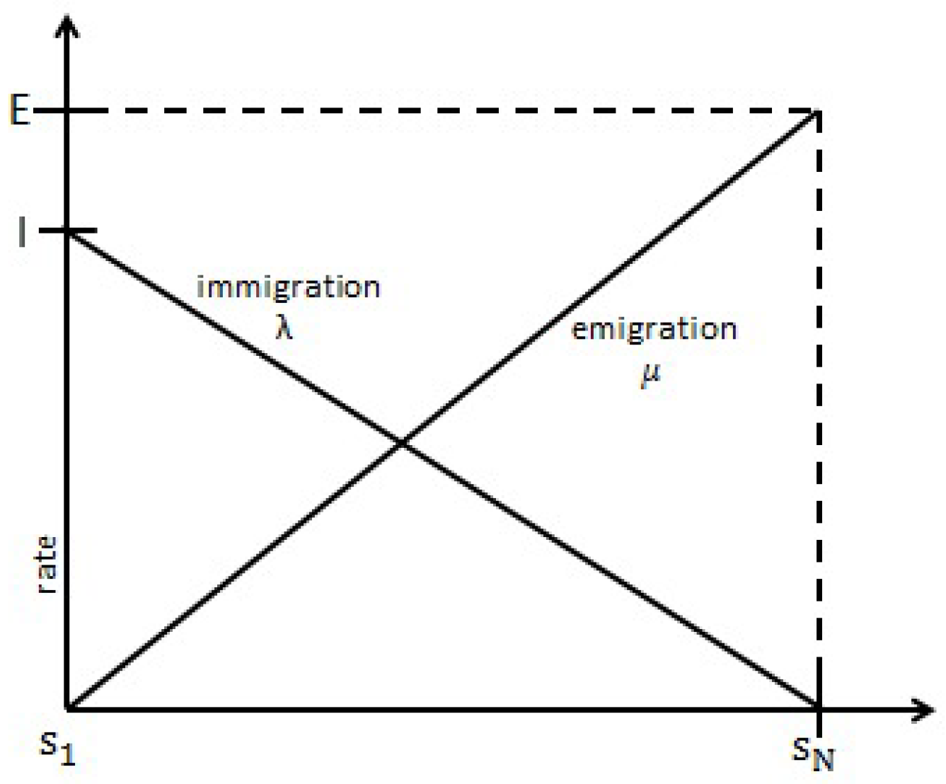
Another example of a metaheuristic algorithm is biogeography-based optimization (BBO). It was developed by Simon (2008); its inspiration is the dynamics of the geography of habitats. It basically consists of migration and mutation. Elitism is also added to ensure faster convergence. BBO has been used to solve numerous optimization problems in the real world. Some newer applications of BBO can be found in Reihanian et al. (2023) and Ren et al. (2023). Those studies concluded that BBO is a very powerful optimizer. For MINLP, Garg (2015) showed the efficiency of BBO in solving reliability problems and the results demonstrated the superiority of BBO over other metaheuristics. In their approach, the integral and discrete constraints were treated as if they were continuous, but in the function evaluation, they were rounded accordingly. This is sensible, because BBO is known for its effectiveness in continuous optimization. One of the reasons why we chose BBO is that it requires minimal parameters and is easy to implement.

For applications in portfolio optimization, there are some entries in the literature that have used BBO as the main optimizer. In Ye et al. (2017), the authors used BBO to solve a portfolio optimization problem with second-order stochastic dominance constraints. In Garg and Deep (2019), the authors used a variant of BBO called Laplacian biogeogeography-based optimization (LX-BBO) to find portfolio allocation from 10 assets in an MV model. In Panwar et al. (2018), the authors used BBO to solve a constrained MV model and applied the results in forecasting via Monte Carlo. The number of assets used in that research was 15.

Over the time, the number of companies listed in the stock markets are increasing. There are many markets with a very large number of companies. Although this provides a good opportunity for investors to choose assets, this also creates the problem in choosing suitable assets. In Perold (2022), the author studied how to efficiently choose a subset of a large set to optimize a portfolio. He considered a constrained portfolio optimization with a cardinality constraint and a quantity constraint. His method was inspired by quadratic programming techniques and was later improved to work very well for solving portfolio optimization. In Qu et al. (2017), the authors considered a multiobjective constrained mean-variance model and used four methods to solve the problem. The methods they used were Normalized Multiobjective Evolutionary Algorithm based on Decomposition (NMOEA/D), Multiobjective Differential Evolution based on Summation Sorting (MODE-SS), and Multiobjective Differential Evolution based on Nondomination Sorting (MODE-NDS), Multiobjective Comprehensive Learning Particle Swarm Optimizer (MO-CLPSO), and Nondominated Sorting Genetic Algorithm II (NSGA-II). The constraint they added to the model was a preselection constraint. They concluded that the methods were efficient for large-scale portfolio optimization. They also suggested adding practical constraints such as the cardinality constraint and the quantity constraint for further research.

In this paper, we proposed the usage of the heuristic ideas of Chang et al. (2000) but implemented in a BBO framework to solve a constrained MV model. The reason we used the ideas of Chang et al. (2000) is that they worked very well on a large-scale portfolio in their study. The dimensions studied by that work were 31, 85, 89, 98, and 225. Their methods could solve a large-scale portfolio optimization problem with high accuracy and in short time. It is clear that standard methods do not solve this problem effectively because the computational complexity is very large.

We used data from ORLibrary, which is available online. The same data were used in Chang et al. (2000) and Kabbani (2022). We also compare our results with theirs using the same performance metric. The results show that BBO is competitive in comparison to other methods.

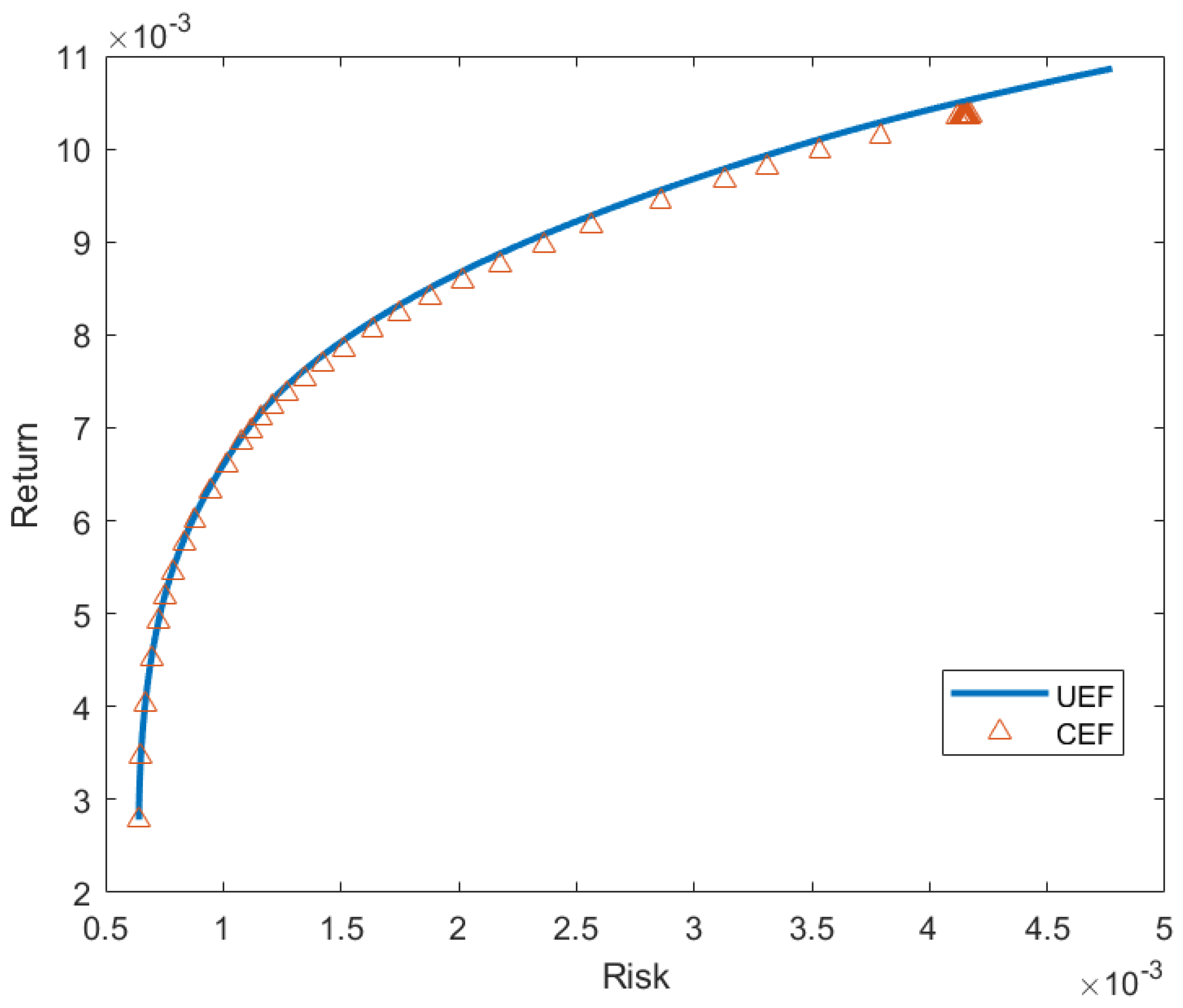
The organization of this paper is as follows. Section 2 introduces the problems that we solve in this paper and how we solve them. The problem is multiobjective constrained portfolio optimization. Then, introduce biogeography-based optimization (BBO) before detailing the method we propose. Section 3 contains the results of our proposed approach and a comparison with other studies. Conclusions and further improvements are also included in that section.

2. Materials and Methods

2.1. Portfolio Optimization

The aim of this subsection is to introduce the problems discussed in the paper. First, we describe the unconstrained MV model. Then, we discuss the constrained MV model. We follow the formulation used in Kabbani (2022).

2.1.1. Unconstrained MV Model

Suppose there are n assets, $A_1,A_2,\dots ,A_n$. Let $x_1,x_2,\dots ,x_n$ denote the budget share or allocation for the assets. The unconstrained MV model can be written as

$$\begin{array}{c}\hfill min\sum _{i=1}^n\sum _{j=1}^n{\sigma }_{i,j}{x}_i{x}_j,\end{array}$$

(1)

$$\begin{array}{c}\hfill \mathrm{s}.\mathrm{t}.\sum _{i=1}^n{\mu }_i{x}_i\ge R,\end{array}$$

(2)

$$\begin{array}{c}\hfill \sum _{i=1}^n{x}_i=1,\end{array}$$

(3)

$$\begin{array}{c}\hfill 0\le x_i\le 1,i=1,2,\dots ,n,\end{array}$$

(4)

where R is the target return, ${\mu }_i$ is the expected return of the ith asset, and ${\sigma }_{i,j}={\rho }_{i,j}{\sigma }_i{\sigma }_j$ is the covariance between the ith and jth asset. Expression (1) indicates the objective is to minimize risk, where variance is taken as the risk measure. Constraint (2) tells that minimum required return is R. Constraint (3) is called the budget constraint, meaning all the budget must be spent in investment. Constraint (4) means the budget share is never negative, so that short selling is not allowed. (1)–(4) altogher is called the unconstrained MV model.

2.1.2. Constrained MV Model

Formally, the constrained MV model is

$$\begin{array}{c}\hfill min\gamma \sum _{i=1}^n\sum _{j=1}^n{\sigma }_{i,j}{x}_i{x}_j-(1-\gamma )\sum _{i=1}^n{\mu }_i{x}_i\end{array}$$

(5)

$$\begin{array}{c}\hfill \mathrm{s}.\mathrm{t}.\sum _{i=1}^n{x}_i=1,\end{array}$$

(6)

$$\begin{array}{c}\hfill \sum _{i=1}^n{z}_i=K,\end{array}$$

(7)

$$\begin{array}{c}\hfill {\epsilon }_i{z}_i\le x_i\le {\delta }_i{z}_i,i=1,2,\dots ,n,\end{array}$$

(8)

$$\begin{array}{c}\hfill 0\le x_i\le 1,i=1,2,\dots ,n,\end{array}$$

(9)

where $z_i\in \{0,1\}$. $z_i=1$ iff the ith asset is in the portfolio. The variable $\gamma$ in expression (5) is the risk attitude parameters. The closer $\gamma$ to 1, the more risk aversity occurs. On the other hand, the closer $\gamma$ to 0, the more risk seeking occurs. So, instead of finding the optimal values to just one value of target return, we will find a set of pareto optimal solutions. Constraint (6) is still the same budget constraint. Constraint (7) is called the cardinality constraint, i.e., the number of assets in the portfolio must be K. Constraint (8) is called the quantity constraint. It is a conditional bound that limits the maximum and minimum of allocation in the individual asset if the asset is in the portfolio.

2.2. Biogeography-Based Optimization

BBO was first introduced by Simon (2008). Biogeography studies the distribution of species over habitats. Biogeography mathematically models the natural process of how species migrate from a habitat to another habitat, how new species emerge, and how species become extinct. Migration consists of two kinds: immigration is the event of new species entering a new habitat and emigration is the event of species leaving a habitat (but not necessarily fully disappear from the original habitat). Each habitat (mathematically expressed as n-dimensional vectors) has its own characteristics. Each characteristic is called suitability index variable (SIV). Basically, SIV are the decision variables in the optimization problem. Habitat suitability index (HSI) is the fitness value of a habitat. HSI measures how supportive a habitat accomodates its species. In optimization problems, HSI is the objective function. Each habitat is ranked based on the HSI, the habitat with higher HSI is ranked better than habitat with lower HSI.

Let $S_1,S_2,\dots ,S_N$ denote N habitats. Habitat $S_i$ has exactly i distinct species. The dth SIV (dth-coordinate) of habitat $S_i$ will be denoted by $S_i\left(d\right)$. Each habitat has its own immigration rate (${\lambda }_i$) and emigration rate (${\mu }_i$). Frequently, linear immigration and emigration rates are used. Guo et al. (2014) listed some of popular migration rate models, such as constant, linear, trapezoidal, quadratic, and sinusoidal models. Each migration model has their own advantages and disadvantages. In addition, they also studied the convergence properties of the BBO algorithm and some techniques on how to improve the convergence of BBO algorithm based on the migration rates. Let E and I denote the maximum emigration rate and immigration rate, respectively, In linear migration rate, we have

$$\begin{array}{c}\hfill {\lambda }_i=I\left(1-\frac{i}{n}\right)\mathrm{and}{\mu }_i=E\left(\frac{i}{n}\right),i=0,1,\dots ,N.\end{array}$$

(10)

This is depicted in Figure 1. High number of species will cause a habitat saturated, resulting its species to search for better habitat and prevent more species to enter the overcrowded habitat. Hence, habitat with big number of species will have big emigration rate and small immigration rate. On the contrary, habitat will a small number of different species has big immigration rate and big emigration rate.

Figure 1. Immigration rate and Emigration rate.

In BBO, habitat with better HSI will have more species, because it is more suitable to live in. In conclusion, a better habitat will affect worse habitat to become better. The migration process in BBO is given by Algorithm 1.

Algorithm 1: Migration

Input n, the dimension of the decision variables $S_k$, current solution $\mu$, emigration rate $\lambda$, immigration rate Process Step 1. let $i=1$ Step 2. If $rand(0,1)>{\lambda }_k$, go to step 5. Step 3. Choose a random habitat $S_l\sim {\mu }_l$. Step 4. Replace the ith coordinate of $S_k$ with the ith coordinate of $S_l$, $S_k\left(i\right)=S_l\left(i\right).$ Step 5. Set $i=i+1$. Step 6. If $i>n$ stop. Otherwise, go to step 3. Output Migrated solution $S_k$.

Another variation of migration process was introduced by Ma and Simon (2011). It has a blending parameter $\alpha$ which makes migration process more random. $\alpha$ can be a constant or randomly chosen at each iteration. In this paper, we use constant $\alpha$. Algorithm 2 describes blended migration algorithm.

Algorithm 2: Blended Migration

Input n, the dimension of the decision variables $S_k$, current solution $\mu$, emigration rate $\lambda$, immigration rate $\alpha \in [0,1]$, blending parameter. Process Step 1. Set $i=1$ Step 2. If $rand(0,1)>{\lambda }_k$, go to step 5. Step 3. Choose a random habitat $S_l\sim {\mu }_l$. Step 4. Perform a blending of immigrating and emigrating habitat using $S_k\left(i\right)=\alpha S_k\left(i\right)+(1-\alpha )S_l\left(i\right).$ Step 5. Set $i=i+1$. Step 6. If $i>n$ stop. Otherwise, go to step 3. Output Migrated solution $S_k$.

Natural events like disaster or pandemic can also happen in a habitat. It can trigger some unpredictable changes in the habitat. In BBO, this is called the mutation process. Mutation is more likely to occur in a habitat with extremely high or low number of species. On the other hand, mutation is improbable in a habitat with medium number of species. The mutation probability of a habitat is

$$\begin{array}{c}\hfill m_i=m_{max}\left(1-\frac{P_i}{P_{max}}\right).\end{array}$$

(11)

$P_i$ denote the probability that a habitat will have species count i and $P_{max}=max\left\{P_i\right|i=1,2,\dots ,N\}$. According to Wei et al. (2022), $P_i$ is given by

$$\begin{array}{c}\hfill P_i=\left\{\begin{array}{cc}\frac{1}{1+{\sum }_{k=1}^N\frac{{\prod }_{l=1}^k{\lambda }_{l-1}}{{\prod }_{l=1}^k{\mu }_l}},\hfill & i=0\hfill \\ \frac{{\prod }_{l=1}^i{\lambda }_{l-1}}{{\prod }_{l=1}^i{\mu }_l}{P}_0,\hfill & i=1,2,\dots ,N\hfill \end{array}\right.\end{array}$$

(12)

Mutation in BBO is performed based on Algorithm 3.

Algorithm 3: Mutation

Input n, the dimension of the decision variables $S_k$, current solution m, mutation probability Process Step 1. Set $i=1$ Step 2. If $rand(0,1)>m_k$, go to step 4. Step 3. Replace the ith coordinate of $S_k$ with a random number inside permissible bounds, $S_k\left(i\right)=rand(lowerbound,upperbound)$. Step 4. Let $i=i+1$. Step 5. If $i>n$ stop. Otherwise, go to step 3. Output Mutated solution $S_k$.

Another essential component in the BBO algorithm is the existence of elitism. In short, elitism is the preservation of optimal habitats. During the elitism process, best habitas (typically a very small subset of high ranked habitats) from previous generation will replace the worst habitats in next generation. This procedure ensures next generation best habitats are not worse than the previous generation best habitats. In their study, Ma et al. (2014) proved an interesting result about the convergence of the BBO algorithm for binary problem. The existence of migration and mutation operators without elitism do not guarantee convergence of the BBO algorithm. However, migration and mutation operators combined with elitism will almost surely produce a convergent solution. Hence, elitism is an essential part of the BBO algorithm. In general, the BBO algorithm follows Algorithm 4.

Algorithm 4: Biogeography-Based Optimization

Input $MaxGen$, maximum number of generations N, number of habitat n, dimension of the decision variables E, maximum emigration rate I, maximum immigration rate $m_{max}$, maximum mutation rate $keep$, number of preserved habitats $\alpha$, blending parameter if Blended BBO is used Process Step 1. Initialise randomly N habitats in ${\mathbb{R}}^n$. Step 2. Evaluate the HSI of each habitat and sort the habitats according HSI. Step 3. Calculate $\lambda ,\mu ,$ and m. Step 4. Set $iter=1$. Step 5. For $i=1,2,\dots ,N$, perform migration according to Algorithm 1 or 2. Also, perform mutation according to Algorithm 3. Step 6. Sort the new habitats based on HSI. Step 7. Replace the last $keep$ habitats with the first $keep$ habitats from previous generation and resort the new population. Step 8. $iter=iter+1$. If $iter>maxgen$, stop. Otherwise, go to step 5. Output Return $S_{best}$ (habitat with best HSI) as the best solution.

2.3. Modified BBO

One technique to solve a constrained optimization problem is using penalty function. But, excessive number of penalty functions will have negative effects in the computational complexity. It also reduces the ability to explore and exploit feasible solutions. Most the time, large amount of candidate solutions are not feasible. A large number of iterations are needed to achieve a convergent solution. For portfolio optimization, Chang et al. (2000) developed an efficient scaling algorithm to handle cardinality constraint and quantity constraint at once. Then, the algorithm is embedded inside three optimization algorithms: GA, TS, and SA. Two interesting results from their research are that the solutions produced are both accurate and the algorithms do not require much time.

We propose using the scaling algorithm inside BBO. Furthermore, we implement some heuristic ideas from Chang et al. (2000). One of the methods they used is genetic algorithm (GA) heuristics. Since GA is similar to BBO in some ways, we modify the BBO algorithm following the idea from GA heuristics. In each iteration, rather than checking all habitats one by one, we only do migration from the good habitats. The best habitat is always chosen. Another habitat is chosen randomly only from small subset of best habitats. Furthermore, migration and mutation occurs iff the ith asset exists in both solutions. This greatly simplifies calculation in the BBO algorithm to focus on a subset of assets exist in good portfolio. The scaling algorithm and modified BBO is given below. This strategy is better than handling the integral constraints using penalty in the objective function, because it will require a lot of resources to find a near optimal solution. For example, Febrianti et al. (2022) used a population of 50,000 elements in solving a constrained portfolio optimization consisting of only 5 assets.

Algorithm 5 aims to modify the candidate solution to satisfy the quantity constraint. The idea is to distribute proportionally the weights of assets after ensuring the lower bound is satisfied. Then, for asset weights that are bigger than the upper bound, they are set to be the upper bound. The excesses are distributed uniformly between weights not exceeding upper bounds. Finally, the objective function is evaluated on this valid portfolio allocation. Note that Step 6 modifies the inputted habitat. This step guarantees that the same function value is produced if the processed habitat is inputted again. Algorithm 5 is crucial for the efficiency of the next algorithm.

Algorithm 5: Scaling

Input S, current solution which contains Q, the set of K different assets, and $s_i$, the value for the ith asset. $\epsilon$, the conditional lower bounds. $\delta$, the conditional upper bounds. Process Step 1. Set $L={\sum }_{i\in Q}{s}_i$ and $F=1-{\sum }_{i\in Q}{\epsilon }_i$. Step 2. For $i\in Q$, $w_i={\epsilon }_i+s_i\frac{F}{L}$. $w_i=0ifi\notin Q$. Step 3. $R=\left\{j\right|w_j>{\delta }_j\}$. Step 4. If R is not empty: set $L={\sum }_{i\in Q-R}{s}_i$ and $F=1-({\sum }_{i\in Q-R}{\epsilon }_i+{\sum }_{i\in R}{\delta }_i)$. For $i\in Q-R$, $w_i={\epsilon }_i+s_i\frac{F}{L}$. $w_i={\delta }_i$ if $i\in R$. Step 5. Evaluate the objective function at w. Step 6. Set $s_i=w_i-{\epsilon }_i.$ for $i\in Q$. Output Returns S, objective function value, and w.

In step 1, we generate feasible solutions by first generating random subset consisting of K elements from $\{1,2,\dots ,n\}$. Afterwards, random weights are generated uniformly from $[0,1]$. Afterwards, weights are normalized in order that the sum of weights equals to 1 (budget constraint). The process in Algorithm 6 basically follows the same process as Algorithm 4. The main difference is the Step 5. We choose $BestHabitats$ only from small range of indices, for example $BestHabitats$ can be the set of index $[2,3,\dots ,10]$. Thus, only the good habitats are migrated with the best habitat (habitat with the lowest function value for minimization). This idea greatly simplifies the complexity in each iteration compared than Algorithm 4, where in Algorithm 4, all habitats are considered for migration. The selection is done via roulette wheel selection. Each habitat $S_i(l\in BestHabitats)$ are assigned probability proportional to their ${\lambda }_i$. Subsequently, a random number is generated to determine which habitat is picked for migration. The elitism in Algoritm 6 is also more efficient than Algorithm 4, since only one habitat is replaced in each iteration.

Algorithm 6: Modified BBO for Large Scale Portfolio Optimization

Input $MaxGen$, maximum number of generations N, number of habitats n, dimension of the decision variables E, maximum emigration rate I, maximum immigration rate $m_{max}$, maximum mutation rate $BestHabitat$, limit of the best habitats $\alpha$, blending parameter K, number of assets in the portfolio Process Step 1. Initialise randomly N feasible habitats in ${[0,1]}^n$. Step 2. Evaluate and update each habitat using Algorithm 4. Sort the habitats according HSI. Step 3. Calculate $\lambda ,\mu ,$ and m. Step 4. Set $iter=1$. Step 5. Choose a random habitat $S_j\sim {\lambda }_j$ from $BestHabitats$. Step 6. Create a new habitat $S\ast$ according to blended migration of $S_{best}$ and $S_j$. Step 7. Perform mutation on $S\ast$ according to Algorithm 2. Step 8. If any coordinate of $S\ast$ is negative, replace it with 0. Step 9. Set the assets of $S\ast$ to be the location of positive coordinates. If the number of assets in $S\ast$ is less than K, then randomly add assets from $S_1$ or $S_j$. If the number of assets in $S\ast$ is bigger than K, randomly choose some assets, remove it. Step 10. Evaluate and update $S\ast$ based on Algorithm 4. Step 11. Replace $S_{worst}$ (habitat with worst HSI) with $S\ast$ and sort the habitats based on HSI. Step 12. Set $iter=iter+1$. If $iter>MaxGen$, stop. Otherwise, go to step 5. Output Return $S_{best}$ (habitat with lowest function value for minimization problem) as the best solution.

3. Results and Conclusions

In this section, we first apply the above ideas to measure its effectiveness. We consider using percentage deviation error as the measure of the model effectiveness as used in Chang et al. (2000) and Kabbani (2022). Let $(v_i,r_i)$ denote the pair of variance and return at a point in constrained efficient frontier (CEF) found using proposed method. Let also $(v_j^{\ast },r_j^{\ast })$ denote the point in unconstrained efficient frontier calculated by Chang et al. (2000). For each i, we can find $v_l^{\ast }=max\left\{v_j^{\ast }\right|v_j^{\ast }\le v_i\}$ and $v_u^{\ast }=min\left\{v_j^{\ast }\right|v_j^{\ast }\ge v_i\}$. Then, $r=r_l^{\ast }+\frac{v_i-v_l^{\ast }}{v_u^{\ast }-v_l^{\ast }}(r_u^{\ast }-r_l^{\ast })$ is the approximated return from UEF at $r_i$. The vertical deviation error is calculated using $|\frac{r_i-r}{r}\times 100|$. The horizontal deviation error is calculated in a similar fashion. The percentage deviation error is taken as the minimum of the horizontal and vertical deviation error.

3.1. Results

In this section we solve problem (5)–(9) for 50 values of $\gamma$. We assume $K=10$ (10 assets are chosen for each case), ${\epsilon }_i=0.01$ (the minimum budget allocation for each chosen asset is 0.01), and ${\delta }_i=1$ (maximum budget allocation is 1 for each asset). We use the same dataset as Chang et al. (2000) and Kabbani (2022). In total, there are 5 test instances studied. The data used are the Hang Seng (Hong Kong), DAX 100 (Germany), FTSE 100 (UK), S&P 100 (USA) and Nikkei 225 (Japan) index weekly returns from March 1992 to September 1997. In total, there are 5 test instances studied. For each instance, we generated 50 points, one point for each value of $\gamma$. $\gamma$ will vary from 0 to 1 uniformly with a step length of $\frac{50}{49}$. The parameters used are summarized in Table 1. The comparisons between the proposed method with previous studies are given in Table 2.

Table 1. Parameters in Modified BBO.

Parameter	Value
n	31, 85, 89 98, and 225
$MaxGen$	1500n
N	100
E	1
I	1
$m_{max}$	0.05
$BestHabitats$	$\{2,3,\dots ,10\}$

Table 2. Comparison of performance.

Index	Number of Assets	Error and Time	GA	TS	SA	TS&TR	BBO
Hang Seng	31	Median	1.2181	1.2181	1.2181	1.8120	1.2503
		Mean	1.0974	1.1217	1.0957	2.2656	1.1689
		Time (s)	172	74	79	1154	282
DAX	85	Median	2.5466	2.6380	2.5661	4.2100	2.8845
		Mean	2.5424	3.3049	2.9297	4.0350	2.7018
		Time (s)	544	199	210	2873	1830
FTSE	89	Median	1.0841	1.0841	1.0841	1.2406	1.1232
		Mean	1.1076	1.6080	1.4623	1.2959	1.1056
		Time (s)	573	246	215	2919	1941
S&P	98	Median	1.2244	1.2882	1.1823	2.3630	1.3671
		Mean	1.9328	3.3092	3.0696	2.5068	1.8782
		Time (s)	638	225	242	3107	2310
Nikkei	225	Median	0.6133	0.6093	0.6066	1.3464	2.1840
		Mean	0.7961	0.8975	0.6732	1.2122	2.6556
		Time (s)	1964	545	553	5866	6382

All numerical experiments are done in MATLAB Online. Best numerical experiments are shown in bold.

3.2. Conclusions

This paper discusses the extensions of the classical MV portfolio model to fit proper real-world situations. The extensions include adding cardinality and quantity constraints which are practical for most investors. The lack of decent approaches to solve the problem, especially the large scale ones, stimulates many alternative approaches. We propose the usage of modified BBO to solve the problem. It uses some ideas from Chang et al. (2000) that handle both constraints effectively. The algorithm makes the candidate solutions always satisfy both constraint. This causes the algorithm to yield a convergent result more quickly than letting them evolve wildly.

Table 3, Table 4, Table 5, Table 6 and Table 7 list the points generated by our proposed approach and their average percentage deviation. Figure 2, Figure 3, Figure 4, Figure 5 and Figure 6 shows the unconstrained efficient frontier (UEF) and constrained efficient frontier (CEF) obtained by proposed method. We see that CEF only deviates by a small amount from UEF. From Table 2, we see that modified BBO works pretty well in large scale portfolio optimization. Although GA works best in most instances, modified BBO can still give good near-optimal solutions. Especially, in the third and fourth instances, modified BBO produce lower mean in percentage deviation error than the other methods. The performance of our proposed apporach for the last instance is the worst compared to other methods. To overcome this, more iterations can be performed to the method at the cost of computation time.

Table 3. First and last three optimal portfolios of Hang Seng.

$\gamma$ = 0		$\gamma$ = 0.0204		$\gamma$ = 0.0408
Chosen Asset	Weights	Chosen Asset	Weights	Chosen Asset	Weights
2	0.0100	2	0.0100	4	0.0100
4	0.0100	5	0.9094	5	0.9090
5	0.9097	8	0.0101	9	0.0108
9	0.0101	9	0.0101	12	0.0100
12	0.0100	12	0.0100	15	0.0100
13	0.0100	15	0.0100	19	0.0100
20	0.0100	19	0.0100	20	0.0100
24	0.0100	20	0.0100	23	0.0101
27	0.0100	26	0.0100	26	0.0100
29	0.0102	29	0.0104	29	0.0100
Return	0.0103	Return	0.0103	Return	0.0103
Risk	0.0042	Risk	0.0041	Risk	0.0041
$\gamma$ = 0.9592		$\gamma$ = 0.9796		$\gamma$ = 1
Chosen Asset	Weights	Chosen Asset	Weights	Chosen Asset	Weights
5	0.0408	5	0.0210	2	0.0146
9	0.0288	13	0.0434	13	0.0461
13	0.0323	15	0.1035	15	0.0761
15	0.1176	16	0.0697	16	0.1068
16	0.0257	17	0.0183	17	0.0476
26	0.1693	26	0.1583	26	0.1437
28	0.2825	28	0.2965	28	0.3044
29	0.1688	29	0.1195	29	0.0636
30	0.0870	30	0.1169	30	0.1335
31	0.0472	31	0.0530	31	0.0635
Return	0.0103	Return	0.0034	Return	0.0028
Risk	0.0042	Risk	$6.4848\times {10}^{-4}$	Risk	$6.4228\times {10}^{-4}$

Table 4. First and last three optimal portfolios of DAX.

$\gamma$ = 0		$\gamma$ = 0.0204		$\gamma$ = 0.0408
Chosen Asset	Weights	Chosen Asset	Weights	Chosen Asset	Weights
2	0.0102	2	0.0108	2	0.0100
11	0.0101	11	0.0100	13	0.0151
13	0.0110	13	0.0120	29	0.0118
15	0.0100	29	0.0127	37	0.0100
29	0.0141	38	0.9043	38	0.9031
30	0.0100	41	0.0100	41	0.0100
37	0.0112	47	0.0100	43	0.0100
38	0.9032	57	0.0100	46	0.0100
49	0.0101	74	0.0101	47	0.0100
74	0.0102	77	0.0100	69	0.0100
Return	0.0093	Return	0.0093	Return	0.0093
Risk	0.0024	Risk	0.0024	Risk	0.0024
$\gamma$ = 0.9592		$\gamma$ = 0.9796		$\gamma$ = 1
Chosen Asset	Weights	Chosen Asset	Weights	Chosen Asset	Weights
2	0.0952	2	0.0915	2	0.0711
4	0.1123	4	0.1880	4	0.2193
13	0.1490	13	0.0966	12	0.0450
15	0.0730	19	0.0538	13	0.0541
29	0.1015	29	0.0565	19	0.0993
38	0.0573	49	0.1292	49	0.1103
49	0.1221	51	0.0594	51	0.0818
57	0.0731	59	0.0666	59	0.0664
68	0.1462	68	0.1759	68	0.1773
71	0.0703	71	0.0825	71	0.0747
Return	0.0047	Return	0.0033	Return	0.0025
Risk	$1.9717\times {10}^{-4}$	Risk	$1.5951\times {10}^{-4}$	Risk	$1.4872\times {10}^{-4}$

Table 5. First and last three optimal portfolios of FTSE.

$\gamma$ = 0		$\gamma$ = 0.0204		$\gamma$ = 0.0408
Chosen Asset	Weights	Chosen Asset	Weights	Chosen Asset	Weights
1	0.0101	10	0.0126	5	0.0100
2	0.0102	18	0.9056	9	0.0103
6	0.0100	19	0.0100	10	0.0113
9	0.0100	29	0.0114	18	0.9042
10	0.0100	44	0.0101	19	0.0100
18	0.9038	55	0.0100	26	0.0100
29	0.0133	66	0.0100	29	0.0141
37	0.0124	71	0.0104	44	0.0100
55	0.0100	72	0.0100	55	0.0100
82	0.0100	76	0.0100	68	0.0100
Return	0.0079	Return	0.0079	Return	0.0079
Risk	0.0013	Risk	0.0013	Risk	0.0013
$\gamma$ = 0.9592		$\gamma$ = 0.9796		$\gamma$ = 1
Chosen Asset	Weights	Chosen Asset	Weights	Chosen Asset	Weights
2	0.1848	2	0.1534	2	0.1264
25	0.0688	25	0.0987	20	0.0812
30	0.1028	30	0.0828	25	0.0949
41	0.0555	41	0.0922	30	0.0707
46	0.0911	46	0.1484	41	0.1182
53	0.0943	53	0.0728	45	0.0524
62	0.2044	62	0.1709	46	0.1556
66	0.0634	71	0.0286	62	0.1387
72	0.0524	75	0.0795	75	0.0810
82	0.0826	83	0.0727	83	0.0808
Return	0.0038	Return	0.0033	Return	0.0025
Risk	$2.3204\times {10}^{-4}$	Risk	$2.1689\times {10}^{-4}$	Risk	$2.0841\times {10}^{-4}$

Table 6. First and last three optimal portfolios of S&P.

$\gamma$ = 0		$\gamma$ = 0.0204		$\gamma$ = 0.0408
Chosen Asset	Weights	Chosen Asset	Weights	Chosen Asset	Weights
20	0.0100	12	0.0100	2	0.0100
31	0.0100	14	0.0103	14	0.0104
34	0.0119	20	0.0101	23	0.0100
36	0.0100	34	0.0256	34	0.0266
42	0.0104	42	0.0108	42	0.0103
43	0.0100	55	0.0100	55	0.0100
82	0.9075	56	0.0100	67	0.0100
85	0.0100	82	0.8897	82	0.8878
89	0.0101	86	0.0100	89	0.0149
96	0.0100	89	0.0135	93	0.0100
Return	0.0089	Return	0.0089	Return	0.0089
Risk	0.0025	Risk	0.0025	Risk	0.0025
$\gamma$ = 0.9592		$\gamma$ = 0.9796		$\gamma$ = 1
Chosen Asset	Weights	Chosen Asset	Weights	Chosen Asset	Weights
11	0.0844	11	0.0894	10	0.0604
19	0.0789	34	0.0392	19	0.0895
34	0.0520	36	0.0635	28	0.0648
36	0.0923	37	0.1459	33	0.0568
45	0.1751	62	0.2074	37	0.1504
52	0.0578	64	0.0703	51	0.0797
62	0.1713	65	0.1131	62	0.2530
64	0.0767	73	0.0603	64	0.0763
86	0.1047	86	0.1003	65	0.1001
96	0.1067	96	0.1106	73	0.0691
Return	0.0035	Return	0.0028	Return	0.0018
Risk	$2.3204\times {10}^{-4}$	Risk	$1.4646\times {10}^{-4}$	Risk	$1.3461\times {10}^{-4}$

Table 7. First and last three optimal portfolios of Nikkei.

$\gamma$ = 0		$\gamma$ = 0.0204		$\gamma$ = 0.0408
Chosen Asset	Weights	Chosen Asset	Weights	Chosen Asset	Weights
2	0.0100	9	0.0247	2	0.0104
40	0.0103	40	0.0103	9	0.0119
62	0.0145	62	0.0100	115	0.0134
68	0.0100	79	0.0100	137	0.0100
97	0.0100	104	0.0100	165	0.0105
115	0.0101	114	0.0100	186	0.0100
154	0.0100	115	0.0138	212	0.0100
186	0.0100	165	0.0379	214	0.8937
201	0.0100	201	0.0101	215	0.0201
214	0.9051	214	0.8631	224	0.0100
Return	0.0038	Return	0.0038	Return	0.0038
Risk	0.0015	Risk	0.0014	Risk	0.0015
$\gamma$ = 0.9592		$\gamma$ = 0.9796		$\gamma$ = 1
Chosen Asset	Weights	Chosen Asset	Weights	Chosen Asset	Weights
8	0.0110	60	0.1766	11	0.0802
40	0.0100	97	0.0100	60	0.2004
60	0.2729	98	0.1337	62	0.1656
62	0.2386	114	0.0500	97	0.0141
97	0.1364	129	0.2653	98	0.1519
104	0.0102	162	0.0435	105	0.0617
129	0.0743	165	0.1810	129	0.1305
158	0.0100	196	0.1143	144	0.0100
171	0.1309	215	0.0103	199	0.0100
225	0.1058	225	0.0152	225	0.1756
Return	$8.4069\times {10}^{-4}$	Return	$4.6038\times {10}^{-4}$	Return	$2.5560\times {10}^{-5}$
Risk	$3.4432\times {10}^{-4}$	Risk	$3.4888\times {10}^{-4}$	Risk	$3.1395\times {10}^{-4}$

Figure 2. Constrained Efficient Frontier for Hang Seng.

Figure 3. Constrained Efficient Frontier for DAX.

Figure 4. Constrained Efficient Frontier for FTSE.

Figure 5. Constrained Efficient Frontier for S&P.

Figure 6. Constrained Efficient Frontier for Nikkei.

Possible improvements can be made to the proposed method, such as using ideas of set-based metaheuristic algorithms to take care of cardinality and quantity constraints separately. Such approach has been studied by some researches, for instance see Erwin and Engelbrecht (2020). The idea is to choose a certain subset of assets first, then optimize the portfolio allocation for each subsets. Looking at various migration and mutation models are also interesting direction to do.

Another possible future research is to consider some more practical constraints such as roundlot constraint, transaction cost, preselection constraint, and tracking error constraint. The idea of putting in more constraints is so that investor can fully realizes their investment plans. Overall, the performance of the proposed method is satisfying in solving large scale constrained portfolio optimization.

References

- Bartholomew-Biggs, Mike C., and Stephen J. Kane. 2009. A global optimization problem in portfolio selection. Computational Management Science 6: 329–45. [Google Scholar] [CrossRef]
- Chang, T.-J., Nigel Meade, John E. Beasley, and Yazid M. Sharaiha. 2000. Heuristics for cardinality constrained portfolio optimisation. Computers & Operations Research 27: 1271–302. [Google Scholar]
- Chen, Yi, Aimin Zhou, and Swagatam Das. 2021. Utilizing dependence among variables in evolutionary algorithms for mixed-integer programming: A case study on multi-objective constrained portfolio optimization. Swarm and Evolutionary Computation 66: 100928. [Google Scholar] [CrossRef]
- Erwin, Kyle, and Andries Engelbrecht. 2023. Multi-Guide Set-Based Particle Swarm Optimization for Multi-Objective Portfolio Optimization. Algorithms 16: 62. [Google Scholar] [CrossRef]
- Febrianti, Werry, Kuntjoro Adji Sidarto, and Novriana Sumarti. 2022. Solving Constrained Mean-Variance Portfolio Optimization Problems Using Spiral Optimization Algorithm. International Journal of Financial Studies 11: 1. [Google Scholar] [CrossRef]
- Garg, Harish. 2015. An efficient biogeography based optimization algorithm for solving reliability optimization problems. Swarm and Evolutionary Computation 24: 1–10. [Google Scholar] [CrossRef]
- Garg, Vanita, and Kusum Deep. 2019. Portfolio optimization using Laplacian biogeography based optimization. Opsearch 56: 1117–41. [Google Scholar] [CrossRef]
- Guo, Weian, Lei Wang, and Qidi Wu. 2014. An analysis of the migration rates for biogeography-based optimization. Information Sciences 254: 111–40. [Google Scholar] [CrossRef]
- Jobst, Norbert J., Michael D. Horniman, Cormac A. Lucas, and Gautam Mitra. 2001. Computational aspects of alternative portfolio selection models in the presence of discrete asset choice constraints. Quantitative Finance 1: 489–501. [Google Scholar] [CrossRef]
- Kabbani, Taylan. 2022. Metaheuristic Approach to Solve Portfolio Selection Problem. arXiv arXiv:2211.17193. [Google Scholar]
- Ma, Haiping, and Dan Simon. 2011. Blended biogeography-based optimization for constrained optimization. Engineering Applications of Artificial Intelligence 24: 517–25. [Google Scholar] [CrossRef]
- Ma, Haiping, Dan Simon, and Minrui Fei. 2014. On the convergence of biogeography-based optimization for binary problems. Mathematical Problems in Engineering 2014: 147457. [Google Scholar] [CrossRef]
- Markowitz, Harry. 1952. Portfolio Selection. The Journal of Finance 7: 77–91. [Google Scholar]
- Mavrotas, George, and Kostas Florios. 2013. An improved version of the augmented ε-constraint method (AUGMECON2) for finding the exact pareto set in multi-objective integer programming problems. Applied Mathematics and Computation 219: 9652–69. [Google Scholar] [CrossRef]
- Panwar, Darsha, Manoj Jha, and Namita Srivastava. 2018. Portfolio selection using Biogeography-based optimization & Forecasting. Journal of Advanced Research in Dynamical and Control Systems 10: 852–63. [Google Scholar]
- Parmikanti, Kankan, Sonny Hersona Gw, and Jumadil Saputra. 2020. Mean-Var investment portfolio optimization under capital asset pricing model (CAPM) with Nerlove transformation: An empirical study using time series approach. Industrial Engineering & Management Systems 19: 498–509. [Google Scholar]
- Perold, Andre F. 1984. Large-scale portfolio optimization. Management Science 30: 1143–60. [Google Scholar] [CrossRef]
- Qu, Bo Yang, Qiankun Zhou, J. M. Xiao, J. J. Liang, and Ponnuthurai Nagaratnam Suganthan. 2017. Large-scale portfolio optimization using multiobjective evolutionary algorithms and preselection methods. Mathematical Problems in Engineering 2017: 4197914. [Google Scholar] [CrossRef]
- Reihanian, Ali, Mohammad-Reza Feizi-Derakhshi, and Hadi S. Aghdasi. 2023. An enhanced multi-objective biogeography-based optimization for overlapping community detection in social networks with node attributes. Information Sciences 622: 903–29. [Google Scholar] [CrossRef]
- Ren, Haoyu, Chenxia Guo, Ruifeng Yang, and Shichao Wang. 2023. Fault diagnosis of electric rudder based on self-organizing differential hybrid biogeography algorithm optimized neural network. Measurement 208: 112355. [Google Scholar] [CrossRef]
- Simon, Dan. 2008. Biogeography-based optimization. IEEE Transactions on Evolutionary Computation 12: 702–13. [Google Scholar] [CrossRef]
- Wei, Lisheng, Qian Zhang, and Benben Yang. 2022. Improved Biogeography-Based Optimization Algorithm Based on Hybrid Migration and Dual-Mode Mutation Strategy. Fractal and Fractional 6: 597. [Google Scholar] [CrossRef]
- Ye, Tao, Ziqiang Yang, and Siling Feng. 2017. Biogeography-based optimization of the portfolio optimization problem with second order stochastic dominance constraints. Algorithms 10: 100. [Google Scholar] [CrossRef]
Disclaimer/Publisher’s Note: The statements, opinions and data contained in all publications are solely those of the individual author(s) and contributor(s) and not of MDPI and/or the editor(s). MDPI and/or the editor(s) disclaim responsibility for any injury to people or property resulting from any ideas, methods, instructions or products referred to in the content. |
© 2023 by the authors. Licensee MDPI, Basel, Switzerland. This article is an open access article distributed under the terms and conditions of the Creative Commons Attribution (CC BY) license (https://creativecommons.org/licenses/by/4.0/).