Water and Sheep: The Pronunciation and Geographical Distribution of Two Germanic Vowels in the Dialects Around the Former Zuiderzee Area

Abstract

The Zuiderzee area in the Netherlands is a former inlet sea at the heart of the crossroads of three major regional languages. While these regional languages are largely distinct, previous work by the dialectologist Kloeke indicated similarities due to contact over water, notably the realisation of the Proto-West Germanic vowels *ā and *a. Using various dialectometric methods, we analysed the distribution of these vowels for 121 localities in this region. Specifically, we tried to determine the dialectal landscape more thoroughly, find instances that illustrate cultural diffusion and migration, and evaluate the overall relationship between distance over water and vowel variations. Using a Bayesian population genetic method, admixture, we distinguished nine linguistically explainable clusters, demonstrating its potential. Moreover, we found evidence of cultural diffusion conforming to the overall presence of three different regional languages. Additionally, we employed the so-called matrix method in linear-mixed effects regression to demonstrate that the geographic distance helped to explain the geographic patterns of vowel variation. The distance over water was as effective a measure as the distance over land. We expect this to be common in areas with a history of intensive and sustained shipping traffic.

1. Introduction

The former Zuiderzee (‘Southern Sea’) area, nowadays called the IJsselmeer, forms the old heart of the Netherlands. No other Dutch landscape has changed so drastically over the last century (Nijboer, 2023). As the old heart of the Netherlands, the Zuiderzee offered a route for Hanseatic cities in the Middle Ages to trade with countries in the north and the east. Later, it became an intensive trade route for the rising Amsterdam in the sixteenth and seventeenth centuries. All ships coming from and going to Amsterdam sailed the Zuiderzee. The transformation of the Zuiderzee was realised by the construction of the Afsluitdijk between 1927 and 1932, a closure dam that definitively separated this inland sea from the incoming North Sea, protecting the hinterland against disastrous floods ever since. After the inland sea became a meer (‘lake’), three large polders were created (the white areas in the map in Figure 1).

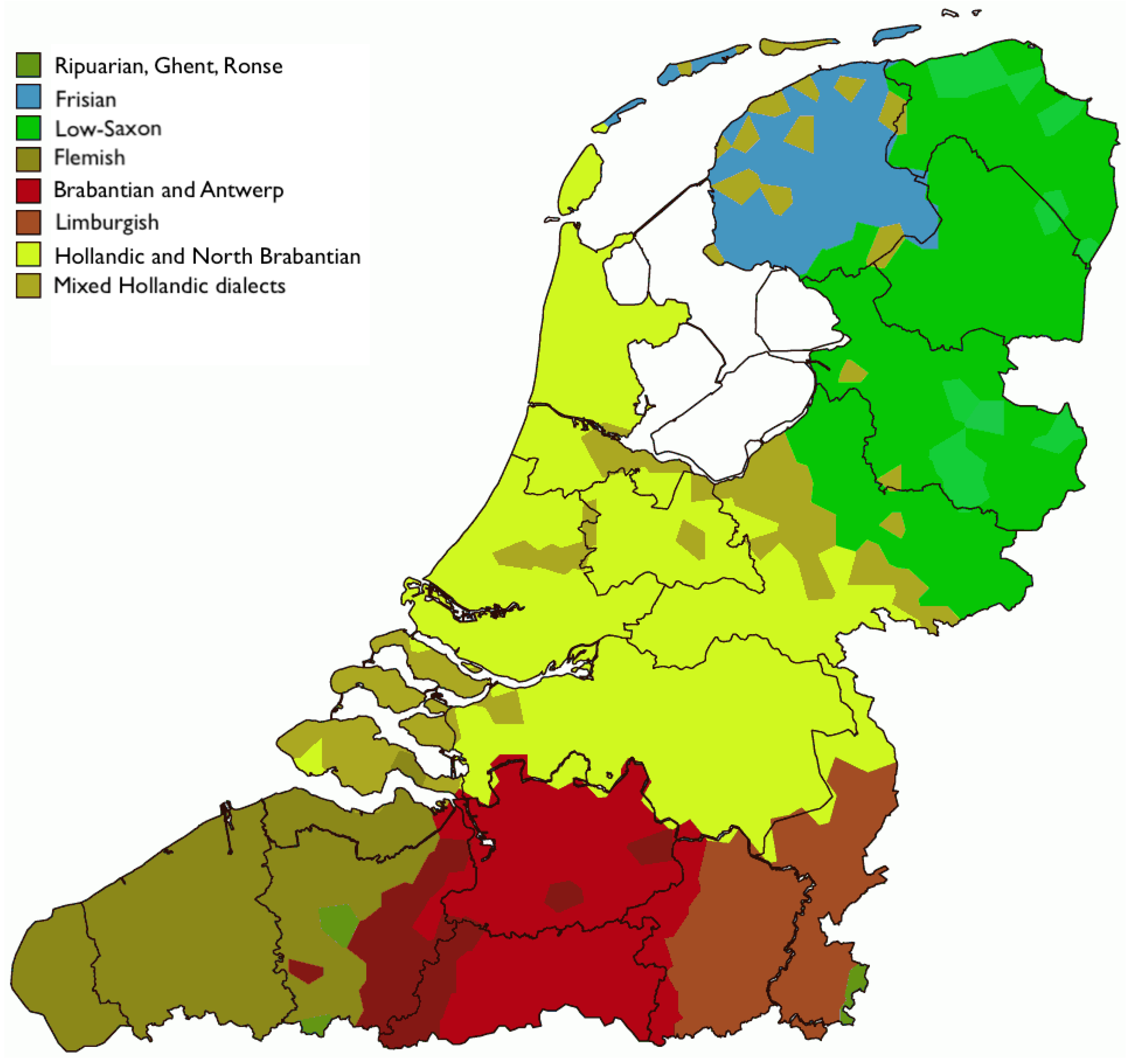
Figure 1 outlines the main dialect areas in the Dutch language area, which covers all of the Netherlands and Flanders in Belgium. As the map shows, the former Zuiderzee is at the crossroads of three regional language areas: Hollandish–Brabantish (in yellow, comprising the Hollandic and Brabantic dialects), Frisian (in blue, comprising the West Frisian dialects), and Low German (in green, comprising the Low Saxon dialects). These three language areas along with their dialects are geographically contiguous, except for the presence of various mixed dialects (in brown) that showcase the supra-regional influence of Hollandish. In addition to those dialects directly bordering the IJsselmeer, mixed Hollandish dialects are found in Friesland, e.g., in Stadsfries (‘Town Frisian’), which developed under Frisian influence in the Frisian localities with town privileges (cf. Versloot, 2021). While Frisian (in blue) is nowadays restricted to just one province, the historical situation was different. In the Middle Ages, the Frisian language was spoken all along the North Sea coast. Over time, other languages replaced Frisian in some areas. The western parts of Frisia came under the supervision of the county of Holland in 1101, and the dominant language spoken in the north of this area became Dutch (Hollandish) with a Frisian substrate. In Groningen (the dark green area in the north-east of Figure 1, right up to the blue Frisian (Fries) area) in the east, Low German (Low Saxon, in green) became the dominant language variety.

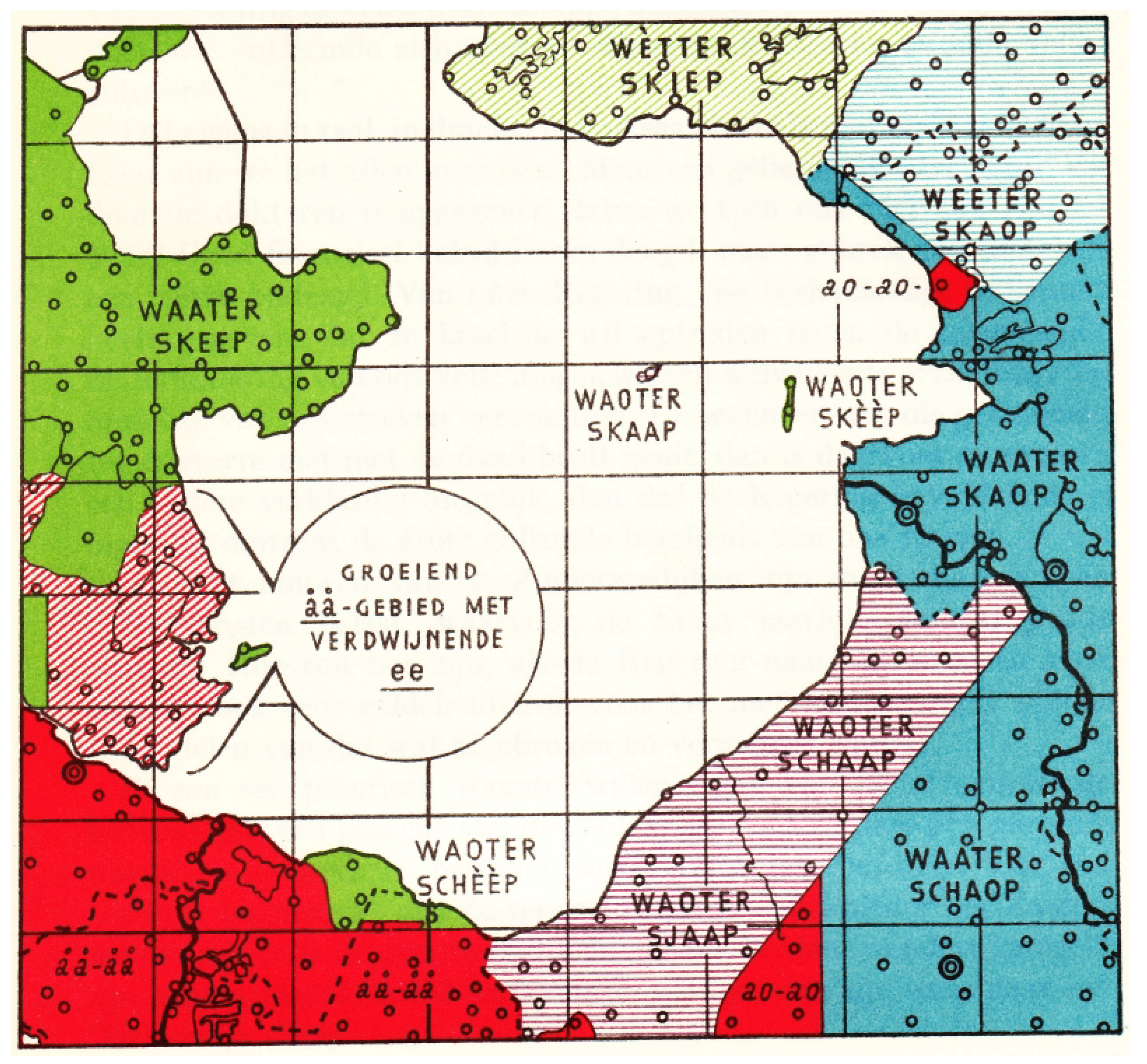
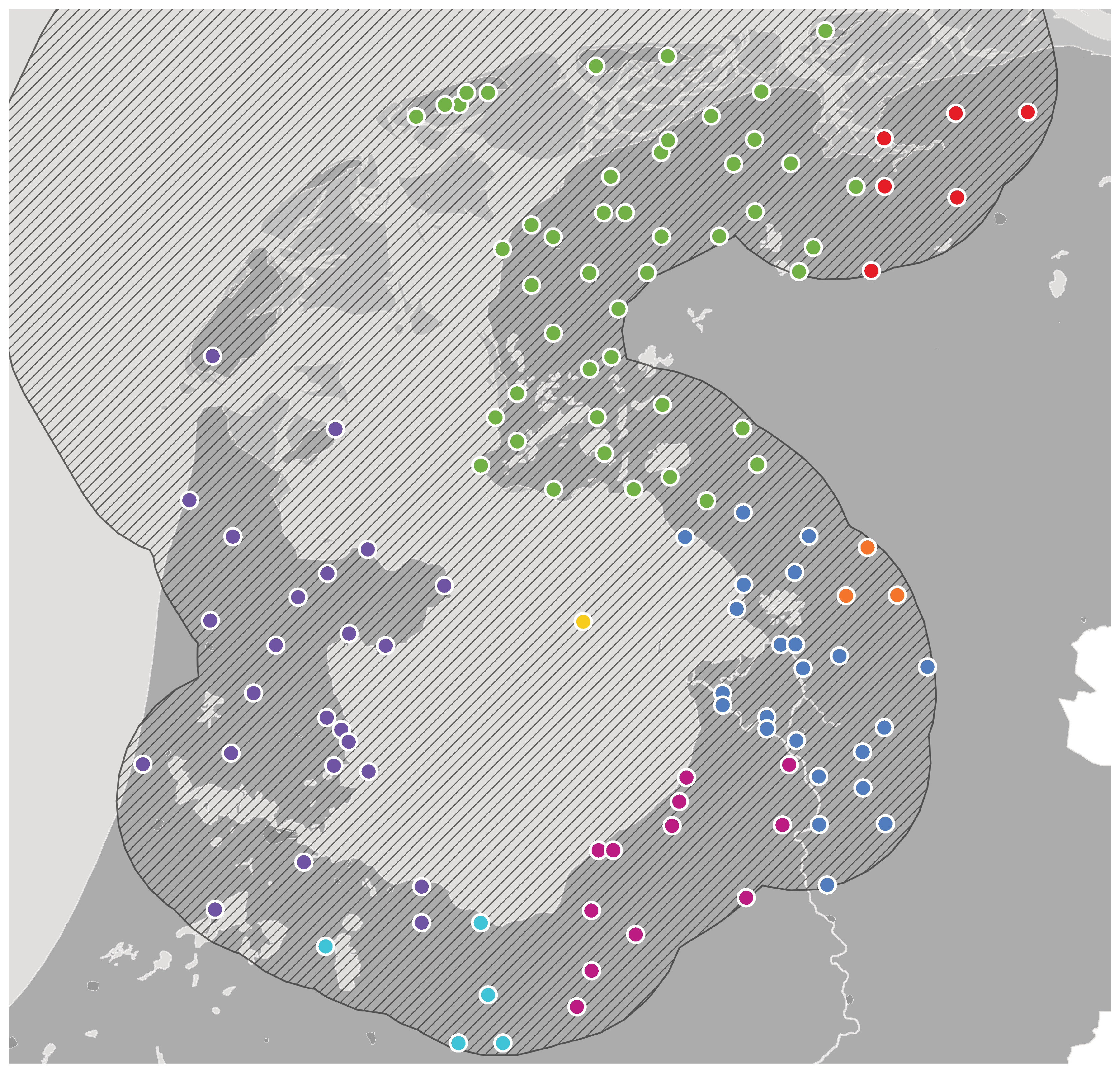
Dialectological research, notably by Kloeke (1934), has revealed complicated patterns of linguistic similarity across localities bordering the Zuiderzee. He investigated the vowels in two words: water (‘water’) and schaap (‘sheep’). Their origins are different, the former descending from the Proto-West Germanic (PWGmc) short vowel *a (which was later lengthened) and the latter from the PWGmc long vowel *ā. The famous dialect map Kloeke made based on his investigation is reproduced in Figure 2 (Kloeke, 1934). Colours were added to visualise the different areas better. The map shows areas where the two vowels merged (as in Standard Dutch; in red) and areas where they were kept distinct (as in, e.g., English; in other colours). The merger between the two German vowels is a well-known development in Standard Dutch (van Bree & Versloot, 2008). This merger is also found in the dialect of Amsterdam and in southern dialects, whereas Frisian and most dialects around the Zuiderzee kept the distinction in various ways (cf. van Bree & Versloot, 2008; Weijnen, 1966)1, as illustrated in detail in the map by Kloeke we have reproduced (Figure 2). The green areas have a close front vowel for ‘sheep’, whereas the blue areas have an open back vowel for ‘sheep’. Apart from the distinctiveness of Frisian (the only area with a close front vowel in ‘water’),2 the patterns of the two vowels do not fully coincide with the dialect areas shown in Figure 1. Overall, the map shows that the reflexes of the two words indicate complicated patterns of linguistic variation surrounding the Zuiderzee.

The patterns of similarities and differences around the Zuiderzee raise the question of how they came about. They seem to be more complicated than a straightforward distinction between the three language areas. What additional explanations, such as migration, diffusion, or contact over water, could be behind them? One interesting case is the former island of Urk, for which the variants ‘WAOTER’ and ‘SKAAAP’ were observed. This pattern differs from the that of the nearest mainland localities in blue. Remarkably, the island to the right, Schokland, is green, while the mainland green area to the left is far away. This island was evacuated in 1859 and the population was relocated to various places around the Zuiderzee. One explanatory factor for this kind of variation could be the distinctive role of contact over water, which may have had a different or supplementary impact in addition to contact over land (Huisman et al., 2019). Over land, interaction tends to be more intense due to a lack of natural barriers, leading to processes of linguistic diffusion over short distances. As a result, neighbouring dialects will differ only slightly (Chambers & Trudgill, 1998). Contact between geographically distant communities will be less frequent, diffusion will occur less, and a dialect continuum will emerge. Nerbonne (2010) investigated language varieties in six areas (Bantu, Bulgaria, Germany, the US East Coast, the Netherlands, and Norway) and found that linguistic differences gradually increased over geographic distance.

What could be the role of an inland sea? The Zuiderzee was a changing landscape during the last few centuries. Sustained contact between communities bordering the sea may have been difficult, blocking communication and separating the three regional language areas. This pattern is what we see in Figure 2. On the other hand, there was a lot of ship traffic in this area, and the islands in its archipelago were not marked as being isolated from ship traffic and contact.

The general linguistic patterns across the Zuiderzee cannot easily be linked to other factors, such as the demography and genetics. Unlike linguistic variation, most major genetic (and, by extension, demographic) variation is observed along a north–south gradient (Abdellaoui et al., 2013; Francioli et al., 2014), broadly reflecting the division between Protestants and Catholics shaped by the major rivers. This division does not align with the traditional threefold linguistic division of Saxon, Frisian, and Hollandic. Recent work (Byrne et al., 2020) confirmed the largely north–south nature of the genetic divisions in the Netherlands but nuanced it by uncovering subtle, more recent divisions along other axes—notably the east–west axis, which coincides very roughly with the linguistic difference between Hollandic and Saxon. The population of the Saxon regions comprises various separate genetic clusters, which indicate isolation. Nonetheless, this does not apply to Frisia, as Frisia genetically aligns with Holland and the northern part of Groningen. On the other hand, a few places in the Zuiderzee are characterised by a highly distinct genetic and demographic profile. The most telling example is Urk, which demonstrates extensive genetic homogeneity and isolation (Somers et al., 2017). Additionally, other places such as Volendam and the former island of Schokland are known to have a presence of unique genetic disorders resulting from prolonged genetic isolation (Madan et al., 1990). Genetic isolation seems—in these places—to coincide with linguistic distinctiveness.

We wanted to investigate the configuration of the language area around the Zuiderzee by using more data than just the two particular words investigated by Kloeke (1934), as they represent two larger groups of words3. The words selected for this study comprised various parts of speech (nouns, verbs, adjectives) and covered both basic vocabulary (e.g., ‘day’, ‘to sleep’, ‘heavy’) and cultural-specific concepts (e.g., ‘Easter’). The words in which the two vowels occur thus provide broad coverage of the lexicon, making them highly representative of the general underlying dynamics of dialectal change in the area. The vowels in these groups of words will likely vary across dialects depending on their etymological origin. Still, we also wanted to take into account their phonological context, as well as external factors like language contact (either through cultural diffusion or migration (cf. Gerritsen & van Hout, 2006)). We used the GTPR (Goeman–Taeldeman–Van Reenen project; Taeldeman & Goeman, 1996) database, available from Gabmap (Nerbonne et al., 2011), to answer the following three research questions:

• Which dialect groups can we distinguish based on the vowels in these two groups of words?
• To what extent do these groups reflect cultural diffusion and migration across the three general regional language areas?
• How can distance in general, and the distance over water in particular, help explain the geographic patterns in vowel variation?

To address the first and second research questions, we applied admixture analysis, a type of model-based clustering method originally developed in population genetics (Patterson et al., 2006; Pritchard et al., 2000). Its aim is to determine how individuals can be classified into populations. In a linguistic scenario, it has been used to classify languages into language (sub)families (Norvik et al., 2022; Reesink et al., 2009) or dialects into dialect groups (Honkola et al., 2018; Syrjänen et al., 2016). The method infers k ancestral populations (here, dialect groups) and models the ancestry of each individual (here, each dialect). Crucially, it allows individuals to have multiple ancestors, i.e., they can be admixtures of multiple populations. Linguistic admixture can be regarded as contact patterns between languages/dialects, thus making this approach a suitable choice for the current study.

Admixture analysis shows which clusters of localities can be distinguished and how typical dialects (individuals) are for these clusters (dialect groups, populations) or how mixed they are. We related the clusters to typical examples of words, but that excluded the mixed dialects. Our next step was to investigate the similarities between the words we selected to obtain more insight into the genetic (linguistic) material. We applied hierarchical cluster analysis to investigate whether all words were really classified as expected on the basis of their historical origin—specific words may have their own, deviant pattern—or whether the distribution of the vowels took a different course. We used the outcomes of this cluster analysis to compute the linguistic distances between the dialects to answer the third research question.

To answer the third research question, we performed a mixed-effects regression analysis, in which we included both the clusters found and the linguistic and geographic distances between the locations involved. This analysis should provide insight into the role of the distance over land and water and geographical clustering (Huisman et al., 2019).

The peculiar situation of the Zuiderzee is (at least partially) reflected in the genetic structure of the Dutch population and the population admixtures around the Southern Sea (Byrne et al., 2020). We focused on the dialect data, of course, and the resulting clusters. To address the second research question, we needed to compare the outcomes to the dialect areas distinguished in the maps in Figure 1 and Figure 2. We hoped to show that admixture analysis contributes to the detection of the different sources (ancestors, migration) of dialect differences and areal differentiation and to test the role of linguistic parameters.

2. Materials and Methods

Given the size of the research area, the number of suitable datasets was limited. Notably, two datasets stood out: the RND and GTRP, each spanning the entire Dutch linguistic area, though they differ in terms of the periods in which they were recorded. The RND contains data on dialectal variation for 141 sentences for 1.956 localities over 59 years (1932–1982) (Blancquaert & Pée, 1925–1982). The RND is only partly digitised.

The GTRP was composed over a much more restricted and more recent timespan (1980–1995). It contains 1876 well-documented and consistently transcribed items (using the international phonetic alphabet) for 613 localities in the Dutch language area (M. Wieling et al., 2007). The items were selected to overcome some of the shortcomings of the RND by using a shorter timespan and a smaller group of transcribers (Taeldeman & Goeman, 1996). Compared to the RND, the GTRP also has better (digitised) coverage in the Zuiderzee area, making it an ideal source for this project. Moreover, as most informants for the GTRP were born before the Second World War, their dialects reflect the pre-polder configuration of the Zuiderzee region and were not the result of recent migration.

The sample from the GTRP dataset we used here came from M. B. Wieling (2007). This sample excluded plural nouns (but kept diminutive nouns), used the base forms of adjectives rather than their comparative forms, and only incorporated first-person plural verbs since other verb transcriptions might have contained pronouns. These constraints were necessary to remove potential problems with segmentation since the border between articles and nouns was not always clear from the transcripts alone. Furthermore, the extensive diacritics system in the original data was omitted in the selected data.

2.1. Selection of Words

The GTRP offers exhaustive etymological data for each item it lists. These data differentiate the originally long West Germanic *ā and the lengthened West Germanic *a. A specific subset of the GTRP data, encompassing only relevant words and locations, was generated using a general filtering script. Separate lists for words with both origins were created based on etymological information. Loanwords and highly related words (e.g., diminutives and standard forms) were excluded for consistency. Only words with an [a:] in all their forms were included (i.e., plurals must have had an [a:] in their singular form).

Table 1. Overview of the GTRP words descended from the Proto-West Germanic long vowel *ā (n = 24) and from the Proto-West Germanic vowel *a (n = 16).

From Proto-West Germanic *ā

From Proto-West Germanic *a

blazen, ‘to blow’; braden, ‘to roast’; draden, ‘wire:PL’; draaien, ‘to turn’; haastig, ‘hasty’; haken, ‘hook:PL’; kwaad, ‘angry’; laag, ‘low’; maanden, ‘month:PL’; maten, ‘measure:PL’; naalden, ‘needle:PL’; raden, ‘to guess’; schapen, ‘sheep:PL’; slaan, ‘to hit’; slapen, ‘to hit’; staan, ‘to stand’; straten, ‘street:PL’; tafels, ‘table:PL’; taai, ‘tough’; traag, ‘slow’; vragen, ‘to ask’; wafels, ‘waffle:PL’; zwaar, ‘heavy’

dagen, ‘day:PL’; dragen, ‘to carry’; gapen, ‘to yawn’; graven, ‘grave:PL’; halen, ‘to fetch’; hanen, ‘rooster:PL’; haver, ‘oats’; jagen, ‘to hunt’; kraken, ‘to crack; creak’; magen, ‘stomach:PL’; maken, ‘to make’; schade, ‘damage’; schaven, ‘to grate’; sparen, ‘to save’; vader, ‘father’; varen, ‘to sail’

presents the words used in the analysis.

2.2. Selection of Localities

In selecting localities to include in this study, we aimed to balance the potential effects of contact over water, language contact through migration, and dialect contiguity, while avoiding the risk of omitting too much of the existing data. After evaluating multiple methods, a balanced set was found by drawing a 20-km buffer around the Zuiderzee coast. This method resulted in a total of 121 localities (see Appendix A for a complete list). Figure 3 presents an overview of the buffer and the resulting localities. We verified the presence of localities mentioned as having distinct dialects in older references, such as Urk, Enkhuizen, and Huizen. For each locality, we coded whether it is directly adjacent to the (Zuiderzee. In addition, considering the significant role of the fishing industry as a source of contact across the Zuiderzee, we coded for each locality whether it has (or had) a sizeable fishing industry. This coding was based on the studies of Ypma (1962) and Bosscher et al. (1973). These two references provide extensive information about the economic importance of fishing around the Zuiderzee. Appendix A provides information about the localities, their adjacency to the Zuiderzee, and their status as a fishing village. The geographic coordinates of the localities in the GTRP dataset were obtained from Gabmap (Nerbonne et al., 2011) and imported into a PostgreSQL database equipped with the PostGIS extension. This environment was the basis for subsequent geographical data processing. Geographical boundaries from Vos et al. (2020), representing the situation in 1850 A.D., were used to define the Zuiderzee area precisely. The resulting map can be seen in Figure 3.

Method

We used Python to process the GTRP data, which were available as a text file showing the dialectal equivalents of Standard Dutch forms. The Python script utilised the geographical processing option from the PostgreSQL extension PostGIS to filter the relevant data from the text files (i.e., localities within the 20-km buffer). The script was designed to output the data in the original Gabmap format to ensure direct usability. Next, these filtered realisations were aligned with the Standard Dutch forms to extract the relevant dialectal realisations. All alignments were obtained with a Levenshtein implementation developed for Buurke et al. (2022). This filtered output with realisations for every word for every locality formed the basis for all the analyses described below.

To cluster the Zuiderzee dialects based on the distribution of the five vowel classes across the target words, we used model-based admixture analysis. The analysis was conducted using the LEA package (Frichot & François, 2015) in R (The R Core Team, 2021). The LEA package uses sNMF (sparse non-negative matrix factorisation) as its inference algorithm, which is based on a fast version of STRUCTURE and which produces results that are similar to those of STRUCTURE (Caye et al., 2016). The algorithm simultaneously infers any k ancestral populations, as well as how the ancestry components are reflected in each individual, without a priori information on how they are related to each other. The resulting ancestry proportions are a probabilistic, non-hierarchical clustering solution. As the optimal number of clusters was unknown beforehand, we conducted the admixture analysis for the k values 1 through 20. We used LEA’s built-in 20-fold cross-validation approach to determine which value of k best fitted the data. In addition, to test the model consistency, we ran 20 repetitions of the analysis for each K value. This evaluation showed that K = 9 was the optimal solution.

We applied mixed regression using the matrix approach developed earlier (see Huisman et al., 2019). The matrix approach enabled the investigation of distance in general, including all the localities. A standard mixed regression required the definition of the distance variable with respect to one fixed point, for instance, Amsterdam, Urk, or Standard Dutch. The matrix approach defined the distance as a property of all the pairs of locations.

2.3. Linguistic Data: Vowel Classes

Across the localities and words studied here, 17 distinct vowel qualities were coded in the GTRP dataset, with frequencies ranging between a single occurrence and almost 2.000 occurrences. Given this large range of occurrences, we recoded the transcribed vowels into a smaller set of vowel classes to reduce excessive complexity. We initially recoded the vowels into four classes based on their articulatory properties (front, central, raised, retracted; Moisik et al., 2012), but added an additional distinction within the front class (close front vs. open front) to better capture the *a–*e split already present in Old Frisian (see Note 2). Figure 4 shows the location of the five larger vowel space categories we finally distinguished: close front, open front, open back, close back, and central. As recoding the vowels into classes reduces the complexity of the data, we tested their reliability using Cronbach’s alpha. We found that $\alpha =0.91$ for the five-category data used in the admixture analysis, which is well above the widely accepted threshold of 0.70 (Nunnally, 1978).

3. Results

3.1. Admixture Analysis: Nine Clusters

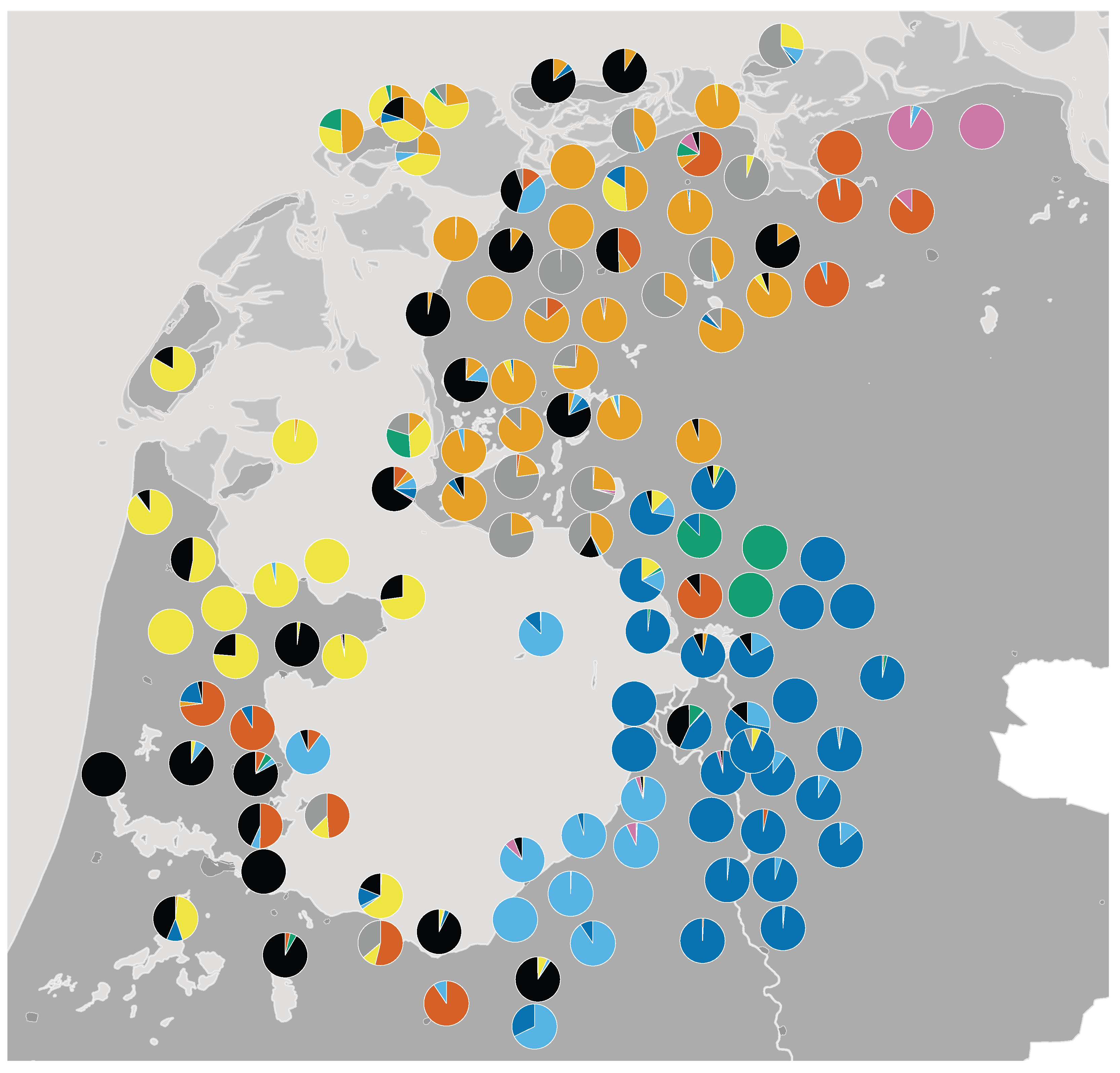
The outcome of the admixture analysis with k = 9 is shown in the map in Figure 5. Each pie chart represents a dialect coloured according to its admixture coefficients (using nine different colours for the nine inferred ancestral populations). If a pie chart only has one colour, this means that this dialect was inferred to have descended from just one of the nine ancestral populations. As the map shows, there was at least one such dialect for each of the nine clusters. If a pie chart has multiple colours, this means the admixture analysis inferred the dialect to be an admixture of two or more ancestral populations. Overall, the results suggested that there were more dialects with some admixture than dialects without any admixture. This was as expected, given the rich history of traffic and contact across this linguistic area.

As is clear from the map, the clusters inferred from the admixture analysis were geographically contiguous and fit earlier typologies of the dialects in the Zuiderzee area. As such, we have tried to name them accordingly in our description (see also

Table 2. Typology of the nine clusters. The vowel column is related to the nine vowel figures and four vowel classes in Figure 6. The vowel classes mentioned here are the single vowel class or two vowel classes indicated in those vowel figures. Constr. indicates the additional type of linguistic constraint active in distinguishing the vowel classes. Cont. and Scatt. indicate whether (part of) the cluster had a contiguous and/or scattered distribution. Both values were positive for the Hollandic cluster, for instance. After assigning all locations to the cluster of their highest admixture coefficient, we made the following split: small (2 or 3 locations), mid (8 to 13 locations), and large (15 or more locations).

Cluster	Map Colour	Vowels	Constr.	Cont.	Scatt.	Size
Frisian I	orange	(1) front closed	fronting	yes	no	large
		(2) back open
Frisian II	grey	(1) front closed	fronting	no	yes	mid
		(2) back open
Frisian	yellow	(1) front open	fronting	yes	yes	large
Hollandic		(2) back open
Low Saxon I	green	(1) front closed		yes	no	small
		(2) back open
Low Saxon II	dark blue	(1) front closed		yes	no	large
		(2) back closed
Reshuffled	light blue	(1) front open	coronal	yes	yes	mid
Saxon		(2) back open
Hollandic	black	open front		yes	yes	large
Merged	red	open back		no	yes	mid
Scattered
Merged	purple	closed back		yes	no	small
Saxon

).

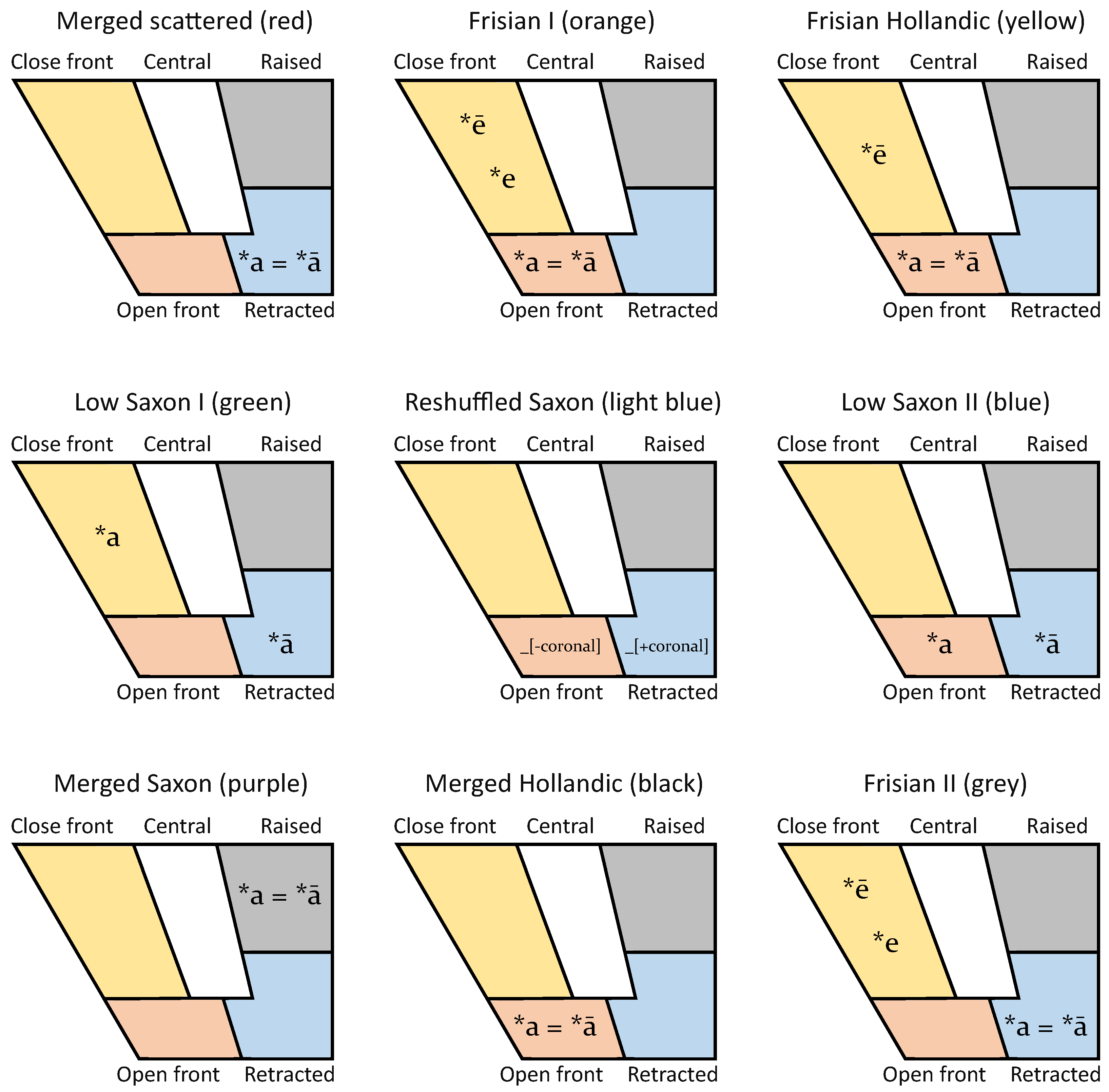
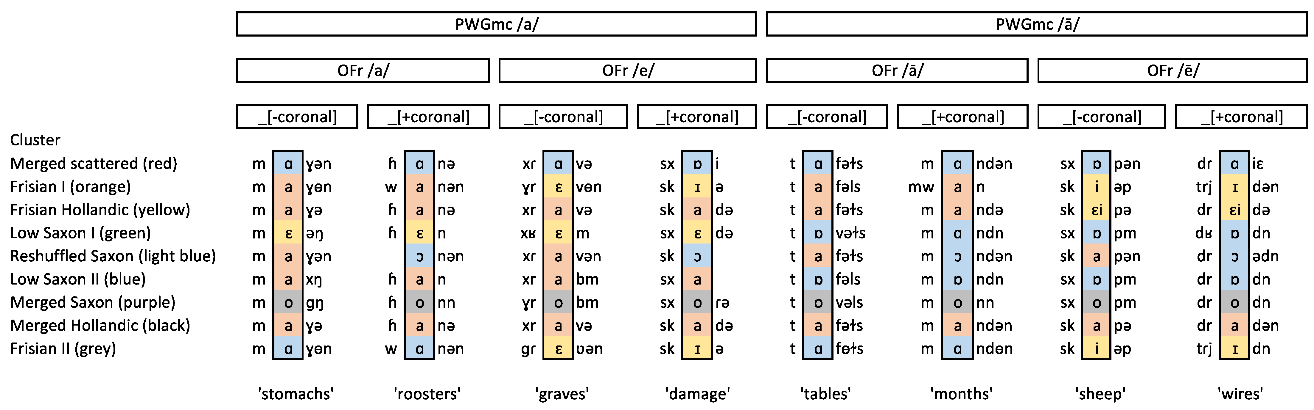
To further interpret the linguistic features underlying the nine clusters, we selected dialects whose admixture coefficient was higher than 0.75 for each respective cluster and qualitatively investigated the vowel classes across different groups of words. The outcome is summarised in Figure 6. These coefficients vary between 0.00 and 1.00. A value of 0.75 indicates that the majority of an individual’s ancestry comes from a single ancestral population. This threshold has been used in a comparable study on Finnish (REF). In our case, almost all the locations (109 out of the 121 locations) had one ancestry component at 0.75 or higher. The vowel panels show how the different Proto-West Germanic vowels were realised across the nine inferred clusters.

The clusters inferred from the admixture analysis can broadly be categorised into three distinct realisation patterns for the Proto-West Germanic (PWGmc) vowels: (1) a Frisian type, with traces of the Old Frisian *e/*ē; (2) a Saxon type, with distinct vowels for *a and *ā; and (3) a merged type, with a single vowel for *a and *ā.

The Frisian I (orange), Frisian II (grey), and Frisian Hollandic (yellow) clusters all displayed a pattern in which we found close front vowels in some, but not all, words where the PWGmc *a/*ā had already been raised to *e/*ē in Old Frisian (OFr)4. These data suggest that OFr *e and *ē are kept distinct in most contemporary dialects (as two different close front vowels). Still, the number of items is too limited to draw definite conclusions. At the same time, all three groups had a merged OFr *a and *ā, but with some differences in their realisation: an open front vowel in the orange and yellow clusters and a retracted vowel in the grey cluster. Geographically, these dialects were found where one would expect them: members of the Frisian I and II groups were found on the mainland of Friesland and on the island of Schiermonnikoog, where a highly distinctive Frisian dialect is spoken. Members of the Frisian Hollandic group were found in the adjacent coastal areas in the west, including the islands of Texel and Terschelling.

The Low Saxon I (green) and Low Saxon II (dark blue) clusters comprised dialects where the PWGmc *a and *ā were kept distinct. Both groups realised *ā as a retracted vowel, but they differed in their realisation of *a: close front in the Low Saxon I group and open front in the Low Saxon II group. A third cluster that could be considered part of this pattern was named Reshuffled Saxon (light blue). Here, we found two realisations of *a and *ā, but not along the lines of the PWGmc categories. Instead, a new distinction appears to have developed here, where *a/*ā is realised as a retracted vowel when followed by a coronal consonant but as a front vowel when followed by other consonants. Members of all three groups were found on the east side of the Zuiderzee (including Urk), with the notable exception of Volendam in the west. Low Saxon I (green) can be seen as a subgroup of the Low Saxon II group, as its size and spread are considerably smaller.

The dialects assigned to the remaining three clusters had a merged PWGmc *ā and *a (as in Standard Dutch). In the Merged Hollandic cluster (black), the merged vowel category was realised as an open front vowel. Dialects belonging to this group were mostly found in the west, but they also included the Town Frisian dialects (known for their Hollandic influence) and the island of Ameland, which had a large influx of Hollandic-speaking shipping crew. The Merged Saxon cluster (purple) was found in the north-east and showed a distinctive raised vowel. Finally, we named the red cluster Merged Scattered, as its members were geographically scattered. The groups comprised both Hollandic and Saxon lects in which the merged *a/*ā category was realised as a back vowel. A closer inspection of the data revealed that the vowel quality differed according to the region (/ɒ/) in the western region, /ɑ/ in the middle region, and /ɔ/ in the north-eastern region), which suggests that their grouping was in part due to recoding the vowels into five broader classes.

Figure 6 and Figure 7 summarise the vowel realisations, split by their etymological origin, across the nine clusters, as well as exemplars for eight different word classes from a typical member of each group.

3.2. Admixture Across Fishing vs. Non-Fishing Villages

As Figure 3 shows, there was some variation in the admixture level inferred for each dialect. Some dialects were assigned to just one ancestral population, whereas others were assigned to two or three (or even more) ancestral populations with different ratios. If we see admixture as the result of contact between dialects, a dialect with zero admixture can be seen as a ‘pure’ descendant of an ancestral population. On the other hand, dialects that show some level of admixture can be seen as dialects in which some outside influence is evident. In the current linguistic area, we expected a difference between fishing and non-fishing villages. Fishing villages can be expected to show higher levels of contact—i.e., admixture—due to increased interaction with their fellow fishing localities. We squared each admixture coefficient to quantify this, summed the squares, and subtracted the sum from 1. This overall admixture score is akin to many diversity/differentiation indices developed in various fields. The measure was 0 if a dialect was assigned to just one ancestral population and maximal if it was assigned to all nine ancestral populations in equal proportions. While the average admixture score for fishing villages ($M=0.32,SD=0.24$) was higher than for non-fishing villages ($M=0.22,SD=0.21$), this difference was not significant ($t\left(119\right)=1.85$, p = 0.066, Cohen’s $d=0.44$).

3.3. Variation Between Words and Word Clusters

We applied a hierarchical cluster analysis (SPSS, Ward’s method, chi-square distance) to the words, applied to the frequencies of the three most frequent vowel classes. The input for the analysis was the vowel value for 40 words for 121 places, obtained by counting their frequencies. We analysed the clustering in the words. We omitted the central vowel class and the raised retracted vowel class (see Figure 4), which both had an extremely low frequency (respectively, n = 43.1% of all occurrences and n = 88.2% of all occurrences). They did not have a relevant effect on the outcomes of the cluster analysis. The result was four clusters, nicely split up between words descending from the PWGmc short *a and long *ā forms on the one hand and words that were or were not affected by Anglo-Frisian brightening on the other. The main mismatch here was traag (‘slow’), which was grouped together with other short-vowel words, even though it is descended from a form with a long vowel (*trāgi).

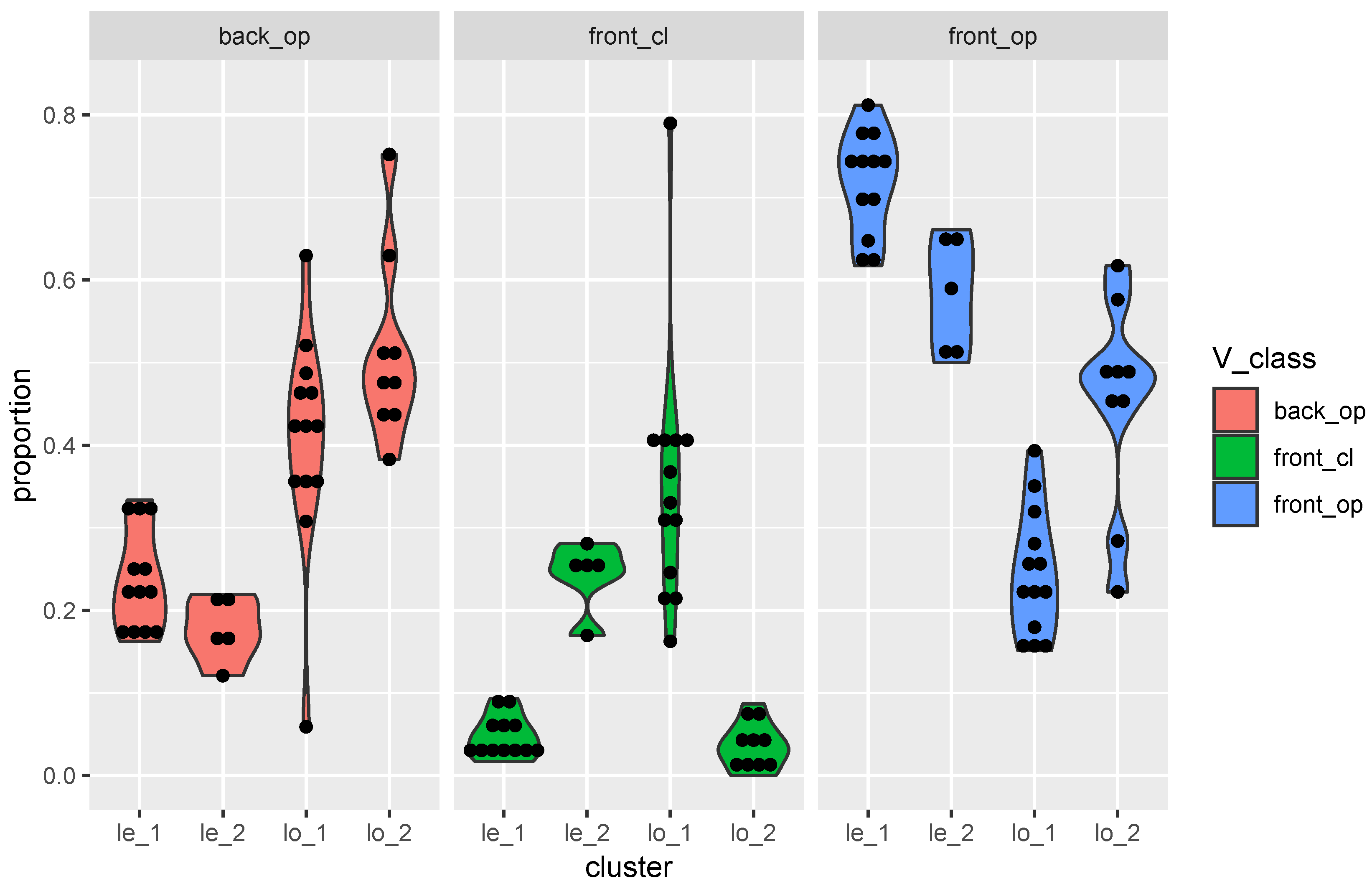
We visualised in Figure 8 the differences between the clusters in violin plots. Clusters 3 (le_1) and 4 (le_2) behaved similarly in terms of having many front–open occurrences, but cluster 3 had the most front–open realisations. Anglo-Frisian brightening (see Note 2) was visible in cluster 2, lo_2, having the consequence that this cluster had more front–open realisations than cluster 1, lo_1. The last two clusters, 1 and 2, had more back realisations. There was one cluster or class shift, the word traag, which shifted from cluster 1 to 3.

In general, we saw that the four clusters described in

Table 3. Overview of the four word clusters with the main split between words descended from the PWGmc *ā and from the PWGmc *a; the only exception is the word traag, which moved from the left column to the right column; the first two words in each of the four clusters are the typical examples in Figure 6.

Frisian	Proto-West Germanic *ā	Proto-West Germanic *a
*a > a	Cluster 1, lo_1 maanden, ‘month:PL’; tafels, ‘table:PL’; haastig, ‘hasty’; maten, ‘measure:PL’; slaan, ‘to hit’; staan, ‘to stand’; taai, ‘tough’; traag, ‘slow’; vragen, ‘to ask’; wafels, ‘waffle:PL’	Cluster 3, le_1 magen, ‘stomach:PL’; hanen, ‘rooster:PL’; dagen, ‘day:PL’; gapen, ‘to yawn’; haver, ‘oats’; jagen, ‘to hunt’; maken, ‘to make’; schaven, ‘to grate’; sparen, ‘to save’; vader, ‘father’; varen, ‘to sail’; shift: traag, ‘slow’
*a > e	Cluster 2, lo_2 draaien, ‘to turn’; schapen, ‘sheep:PL’; blazen, ‘to blow’; braden, ‘to roast’; draden, ‘wire:PL’; haken, ‘hook:PL’; kwaad, ‘angry’; laag, ‘low’; naalden, ‘needle:PL’; raden, ‘to guess’; slapen, ‘to hit’; straten, ‘street:PL’; zwaar, ‘heavy’	Cluster 4, le_2 graven, ‘grave:PL’; schade, ‘damage’; dragen, ‘to carry’; halen, ‘to fetch’; kraken, ‘to crack, creak’

behaved distinctively, but it was also clear that there was a considerable amount of variation even within those clusters. This word-specific variation was reflected in the relatively high level of admixture found for many localities. This indicates that several processes were active, including levelling effects from Hollandish and Standard Dutch influences. It also seems to reveal that contacts and traffic were important in this area.

3.4. Mixed Regression and Distances

The admixture analysis revealed nine dialect clusters across the three regional language areas around the Zuiderzee. Their characteristics were a combination of historical processes (descent from Proto-West Germanic) and linguistic restructuring (e.g., the coronal distinction in the Reshuffled Saxon cluster), as well as dialect levelling (the disappearance of any distinction) due to, e.g., standard language influence. At the same time, we observed that several clusters were rather scattered, whereas others were more contiguous. What additional explanatory power does geographic distance have for this clustering? We decided to use a matrix mixed-effect regression, as explained and tested in Huisman and van Hout (2023).

The first issue to deal with was how to measure the geographic distance. Which traffic routes brought people in contact with each other, and how were they travelling? How much time did this travelling take? These are fundamental questions, but hard to answer. Given the lack of adequate historical sources that take all these factors into account, we measured the geographic distance in the simplest way possible: as the crow flies. We did not consider old or existing traffic routes, nor did we distinguish between travel over water vs. travel over land. In addition, no specific barriers needed to be taken into account for this area. We will return to the appropriateness of this approach in the Discussion.

The next issue was how to measure the linguistic distance. We operationalised this using the four groups of words shown in Table 3 and the relative frequencies of vowel classes across these groups (see Figure 8 for a general overview). For each locality, we determined, for each of the four word groups, the frequency of occurrence of the four vowel categories (close front, open front, open back, and closed back). Then, for each pair of localities, we used these counts to compute, for each word group, the chi-square value. Finally, we calculated the sum of the four chi-square values (one for each word group) as a measure of the overall linguistic distance between a pair of localities.5

Having determined the geographic and linguistic distances between all pairs of localities, we plotted their relation, shown in Figure 9. The figure is a scattergram of the linguistic distance over the geographic distance, with a Loess smooth line added to visualise the pattern of covariation.

Figure 9 shows, overall, that the linguistic distance increased with an increasing geographic distance. This pattern is often found for dialects and is typical of a dialect continuum (Nerbonne, 2010). The correlation between the two measures was 0.366, which can qualify as moderate, meaning there was a considerable number of observations that deviated from the linear pattern. While there were few cases where we found small linguistic distances between pairs of localities that were far apart, we found many pairs of localities that were close to each other but which showed large linguistic distances.

Next, we investigated whether this relationship between the linguistic and geographic distances was the same across the nine clusters. To do so, we assigned each locality to a specific cluster based on its highest admixture coefficient. Figure 10 shows a scattergram with a Loess-smoothed line for each of the nine clusters.

The figure shows some obvious differences between the clusters. The yellow (Frisian Hollandish) and green (Low Saxon I) clusters show a clear, steadily increasing pattern. Several clusters show a plateauing of the linguistic distance (e.g., the Frisian orange and grey clusters). Finally, the clusters comprising dialects in which the two PWGmc vowels were merged (black, red, and purple), show a largely flat line, indicating the absence of a relationship.

To examine the relation between the linguistic and geographic distance in detail, we applied linear mixed-effects regression analysis (lme4 package (Bates et al., 2015) in R), using the full pairwise distance matrices as explained and tested in Huisman and van Hout (2023). In this approach, each locality was compared to every other locality, with a random effect for the reference locality to account for the linguistic uniqueness of each dialect. When we omitted self-comparisons, each of the 121 localities was compared to the other 120 localities, producing a matrix of $121\times 120$ = 14,520 rows.

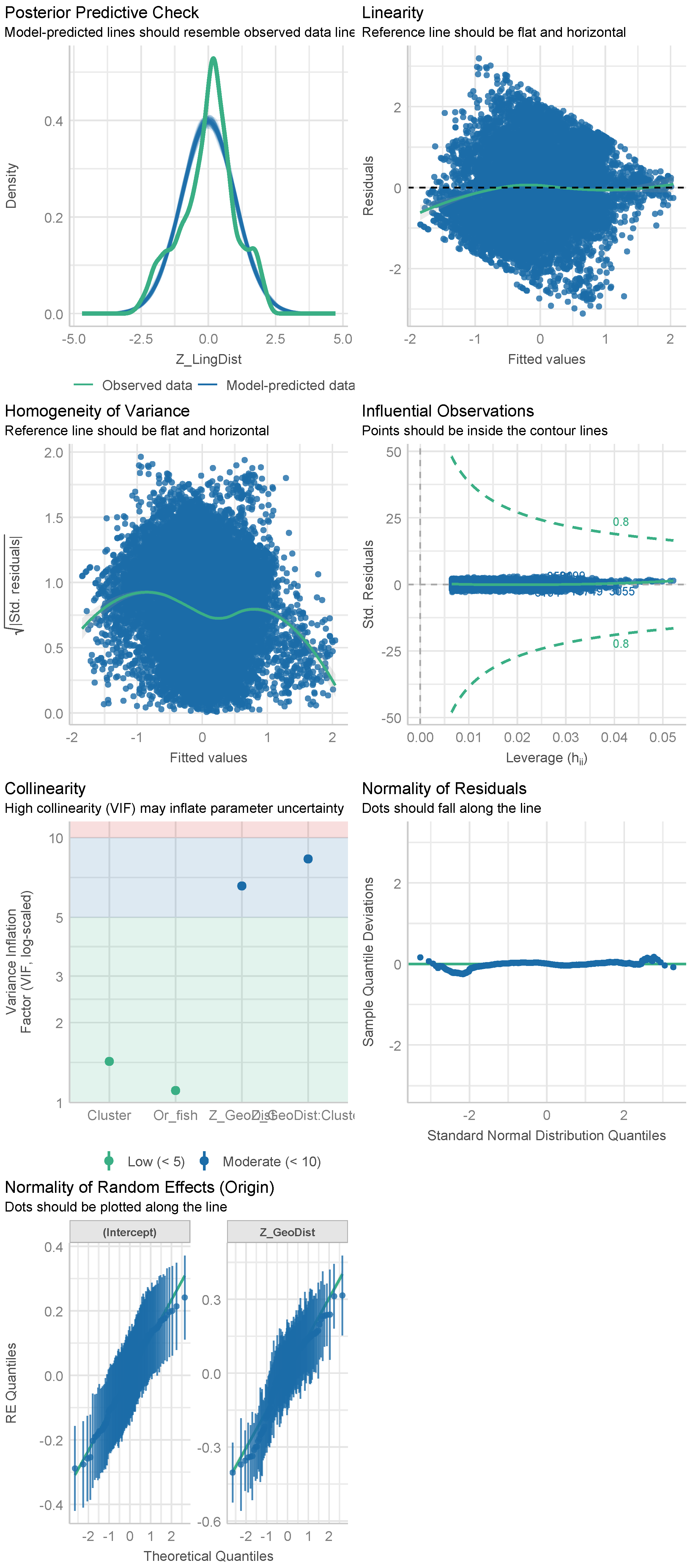
The predictor variables for the linguistic distance were (1) the geographic distance6, (2) dialect cluster membership of the reference locality (nine categories), and (3) whether the locality was a fishing locality (binary yes/no), both for the reference locality and the comparison locality. We added these two variables to test whether fishing localities in the Zuiderzee had a special position. All continuous variables were normalised. We checked the regression assumptions using check_model, a tool that is available in the performance package (Lüdecke et al., 2021). There were no violations. The outcomes can be found in Appendix C.

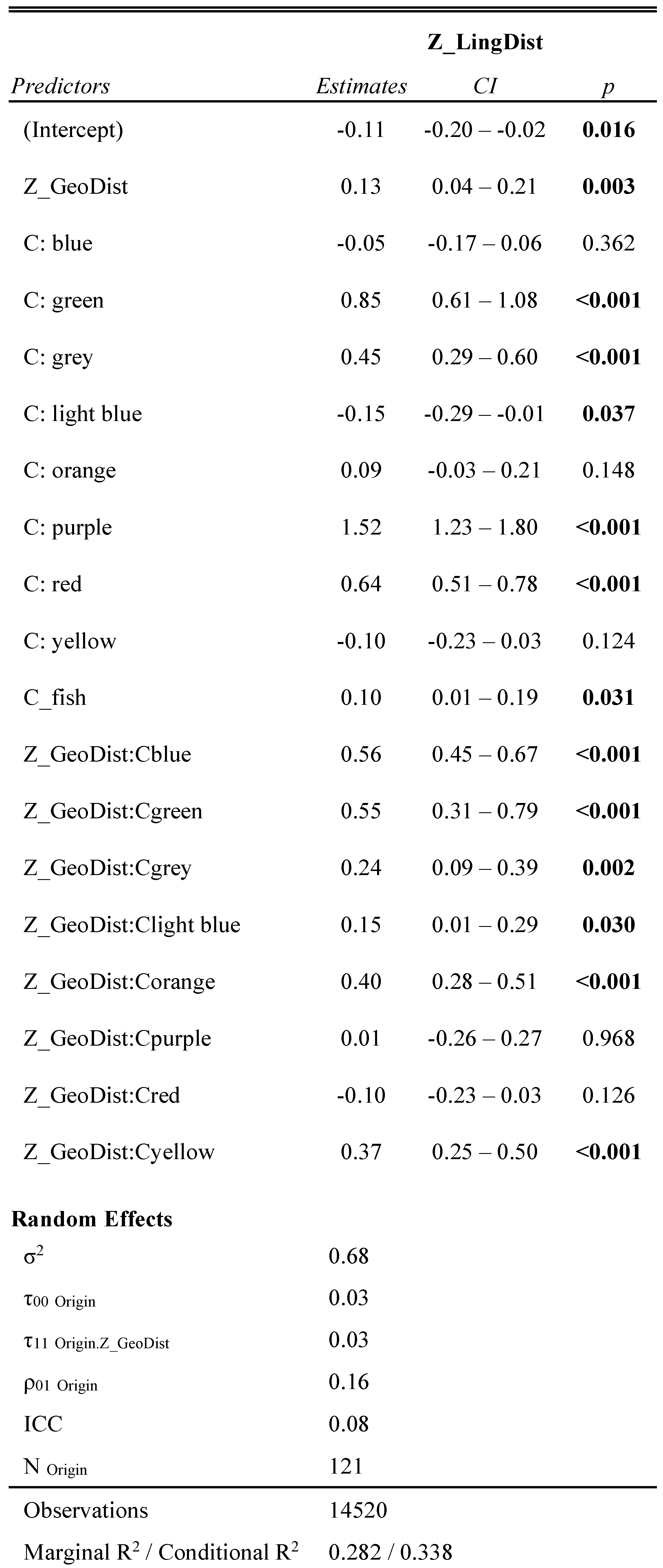
We selected the best-performing model based on the AIC. This model contained the main effects of the geographic distance, dialect cluster membership, and the interaction between the two. In addition, there was a main effect of the fishing locality status for the reference locality. There was a random effect for the reference locality as an intercept, plus a slope for the geographical distance for the reference locality. We also investigated whether a non-linear model performed better, but transformations or polytomous models provided no improvement. We have summarised the outcomes in a table in Appendix B and in Figure 11, which visualises the effect sizes (determined, respectively, by the tab_model and plot_model functions from the package sjPlot (Lüdecke, 2023)).

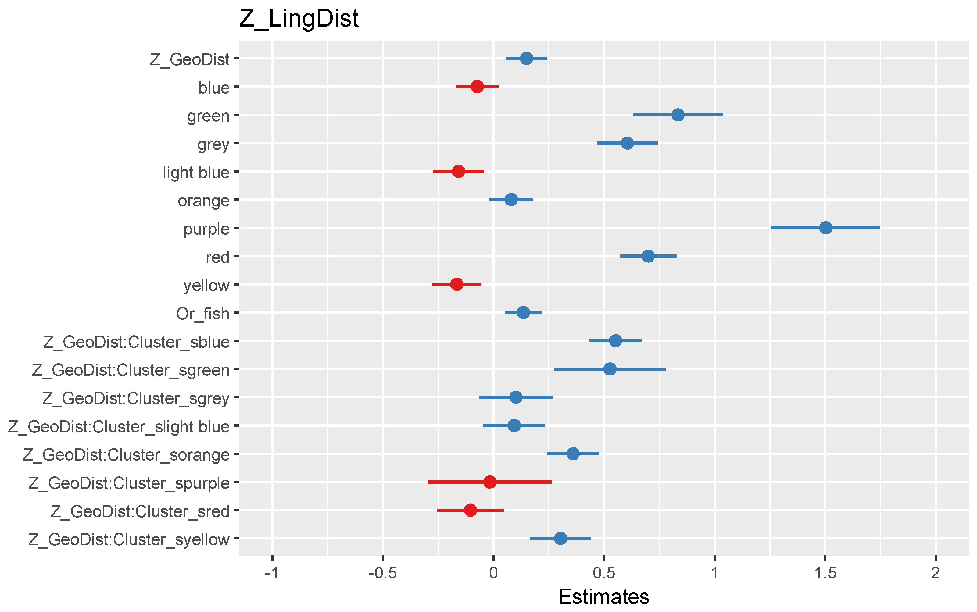
Figure 11 gives a positive main effect for Z_GeoDist, that is, the normalised value of the geographic distance. There was also a positive main effect of the fishing locality status. There were many effects of the clusters and their interaction with the geographic distance. The reference point for their values was the black cluster. These effects are visualised in Figure 12 and Figure 13, along with results from plot_model.

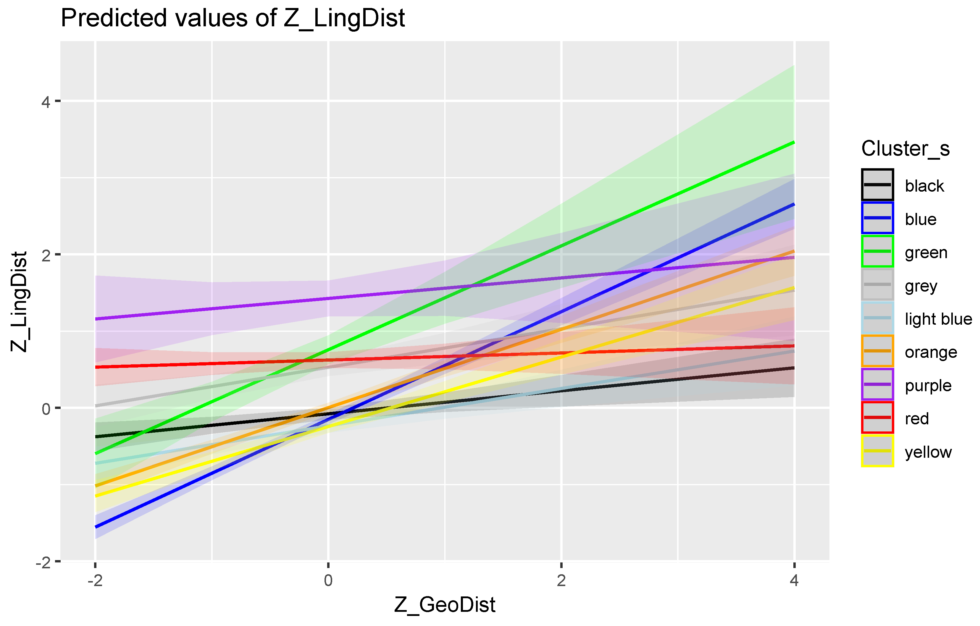
The two Low Saxon clusters (dark blue and green) in Figure 12 show strongly increasing lines, and both have low values for nearby localities, indicating that both clusters are contiguous. The orange and yellow clusters also have a line that is clearly going up. The grey cluster is more scattered, without a contiguous territory. The consequence is a flatter relationship with the distance. The four remaining lines all go up, but their pattern is more flat. The light blue Saxon cluster is scattered in the south part of the Zuiderzee, with the fishing localities of Volendam and Urk as the most conspicuous localities.

The purple, red, and black lines represent merged vowels. The red and black clusters seem to show Hollandish influence. The black cluster in particular illustrates the far-reaching influence of Hollandish, in combination with the dominant position of the Dutch standard language in general. The black cluster shows the impact of expansion and diffusion in a larger area.

Figure 13 confirms the height of the interaction lines’ slopes. The x axis was switched and now represents the nine clusters. The distance between the blue and black spots represents the size of the slope. Moreover, the confidence intervals turned out to be larger for larger distances (the blue spots). There was more variation in the linguistic distance when the geographic distances were larger.

Why was the fishing locality origin significant and not the interaction concerning whether the other locality was a fishing village or not? Such an interaction would have suggested that fishing localities were more alike (compare Volendam and Urk), but that was not what we found as a general effect. We found an additional distance effect, meaning the effect of the distance from other villages was even a bit stronger. Perhaps this indicates their special character. Despite their many contacts, they were closed communities as well.

A last point is the explained variance: the marginal $R^2$ = 0.282 and conditional $R^2$ = 0.338. Both values show that a substantial part of the differences remains unexplained, as indicated by the size of the residual variance.

4. Discussion

In this contribution, we investigated a long-standing issue in Dutch dialectology, the distinction in vowel pronunciation between water, ‘water’, and schaap, ‘sheep’, and its geographic distribution over the Zuiderzee dialects. These two vowels merged in standard Dutch. Originally, their vowels had two different West Germanic ancestors. We extended the analysis to two larger sets of words that we could investigate in an extensive dialect database, the GTRP. We had many representatives of these two ancestor vowel classes, although the word water was missing. The effects of Frisian fronting (Anglo-Frisian brightening) complicated this binary distinction in both vowel classes. In fact, we had to deal with four word classes or clusters.

We applied several dialectometric techniques to unravel the dialect–geographic distribution patterns of the words involved, focalising on their nucleus vowel. We started with the admixture analysis. We obtained nine clusters, with many localities having a mixed pattern of clusters. These mixtures demonstrate the intensive contact between areas and localities. We also applied a hierarchical cluster analysis to the words and completed the analysis with a mixed regression analysis to reveal the interaction of the linguistic and geographic distance in relation to the nine clusters we found. We applied these techniques successfully to obtain an answer to our three research questions:

• Which dialect groups can we distinguish based on the vowels in these two groups of words?
• To what extent do these groups reflect cultural diffusion and migration across the three general language areas?
• How can distance in general, and the distance over water in particular, help explain the geographic patterns in vowel variation?

Three regional language areas, Hollandish (in fact, Hollandish–Brabantish; see Figure 1), Frisian, and Saxon, surround the area of investigation, the old inland sea of the Zuiderzee, in combination with spots and areas with mixed dialects. We found nine clusters. We could assign the clusters to three larger categories: Frisian, Saxon, and merged dialects, including the black Hollandish pattern. We found a Frisian substrate (yellow) in the Hollandic area and a clear Hollandic influence in Friesland and on the island of Ameland. A remarkable Frisian pattern was found for Hindeloopen, in the lower part of Frisia, bordering the Zuiderzee. Its circle contained all three Frisian colours, plus a green Saxon part. van Ginneken (1928) mentions Hindeloopen as a particular dialect and connects its conservative, old Frisian features with its special history going back to the Middle Ages, when the much smaller Flevomeer (meer = ‘lake’) preceded the later Zuiderzee. The red circles were the most scattered cluster. In Groningen, they were neighbours of the small purple cluster. In both the red and purple clusters, the PWGmc vowels *a and *ā merged. We need to investigate the Groningen dialect area in more detail to find out if this merger is typical of the whole north-east region or whether there has been Hollandic influence. The red in the left part of the Zuiderzee area neighbours the black cluster, the difference being the low front vs. back pronunciation of the merged vowel. The answer to research question 1 is that the nine clusters reflect the overall dialect structure of the three regional languages around the old Zuiderzee area, with many traces of mixing, with Hollandish acting as a superstrate language overall, but especially in Frisia, and with Frisian as a substrate language in the Hollandic area.

Nevertheless, both Kloeke (1934) and van Ginneken (1928) emphasised the linguistic unity of the Zuiderzee area. van Ginneken (1928) went far back in time to define a contiguous linguistic area. Following Winkler (1874), he presumed that the non-Frisian Zuiderzee parts shared a common regional ancestor language, which he called Flevisch, Flevish, that preceded the regional Hollandish and Saxon languages. He mentioned the island of Urk (largely light blue) as the best example of this ancestor language but also referred to the islands of Texel (largely yellow) and Terschelling (largely yellow). Only Urk has the coronal split instead of the PWGmc *a/*ā distinction. Van Ginneken had already mentioned this split (van Ginneken, 1928, p. 61). On the other hand, the light blue area coincides with the mixed dialect area of the map in Figure 1, indicating that this is probably a more recent development and not a trace of a forgotten past.

Kloeke (1934) was interested in the role of cultural expansion. He was interested in the role of Holland, in particular Amsterdam, as the main economic and cultural factor in inducing waves of linguistic diffusion over its surrounding area. The distribution of the black circles corroborates the strong role of expansion, migration, and diffusion, but they have not lead to a common language variety on the shores of the Zuiderzee. There are many traces of traffic and contact given the many mixed patterns in the Zuiderzee localities. The Amsterdam spheres of power were not strong enough to create a contiguous areal string of dialects bordering the Zuiderzee. Both Kloeke (1934) and van Ginneken (1928) did not succeed in finding the common language variety they were looking for.

While the data available demonstrate that linguistic patterns are not necessarily or directly linked to broader demographic and genetic patterns, the presence of genetic similarities between Frisia and Holland could be seen to support the intensive contact between regions around the Zuiderzee and, hence, linguistic contact.

The role of geographic distance is visible in all dialectometric studies, but we have shown an additional possibility: estimating its exact effect, in hard figures. Can distance, in general, help explain the geographic patterns in vowel variation? We defined the distance as the crow flies, both in passing over the mainland and water. We defined the linguistic distance on the basis of four word sets and the frequency of vowel classes used in these four sets. We found an overall distance effect in the whole dataset, but this effect turned out to vary according to the cluster involved. Flat distance effects were found for the three clusters with merged vowels (purple, red, and black). The black and red clusters were too scattered to exhibit a clear distance effect. Interestingly, a small distance effect was found for the light blue cluster with two conspicuous fishing localities, Volendam and Urk. It seems to show that water may have a special influence specific to the dialects involved, but we found no overall effect of water. First of all, we found only an increasing linguistic distance effect for fishing localities, which was small. We found no effect of the overall linguistic distance between fishing localities. Secondly, we applied additional distance analyses, the most relevant one being the analysis where we used both the distance over land and the distance over water. This mixed distance model did not improve the results, meaning that the distance over water is the same as the distance over land, although the distances between localities over water were larger than over land. It is tempting to speculate that the travel time over water was comparable to the travel time over land on foot in older times. Water can be a blocking factor when the distances are large: island languages display a typical isolation pattern due to the geographic isolation of islands (Huisman et al., 2019). The distances over water in the Zuiderzee were large enough to maintain the existence of three regional languages despite the combined influx of Hollandish and the Dutch standard language. This means that we can answer research question 3. The overall distance helped us to explain the geographic patterns of vowel variation in the Zuiderzee area. The distance over water was included and was as effective as the distance over land. We expect this to be common in areas with a history of intensive and sustained shipping traffic. Water might be a building block in defining a dialect continuum.

We applied admixture analysis to vowel class data for two groups of words: the descendants of words with PWGmc *ā and the descendants of words with PWGmc *a. Within each group, it was inevitable that the historical developments of these vowels would be correlated to some degree, irrespective of whether the sound changes came from articulatory drift or from lexical diffusion. While there is undoubtedly some dependency on biology as well, admixture analysis based on genetic data assumes the variation that occurs across genes to be independent. Previous linguistic studies have tried to address this by selecting (e.g., typological) features that are less likely to be dependent on each other (e.g., Norvik et al., 2022; Reesink et al., 2009). Here, we have chosen a different approach, selecting data based on their relevance to established work (e.g., Kloeke, 1934). Our analysis of the word groups (Section 3.3) showed that they were far from uniform, suggesting that complete interrelatedness is not an issue here. However, future studies should evaluate our findings on contact patterns across the Zuiderzee using different—more independent—linguistic data.

How successful was our mixed regression analysis in terms of the explained variance? We reported a marginal $R^2$ of 0.282 and a conditional $R^2$ of 0.338. We are satisfied, given the remaining differences between the localities. We performed supplementary analyses, but there were no really outlying places. That does not preclude that local dialects can have their own developments and that localities may be or remain fairly isolated, in contact and in culture. This can be investigated in future research. The same applies to the individual words. There was still a lot of variation between the words, and the words may even betray their origin (cf. the word traag). This fits an old maxim in dialectology: each word has its own history.