Efficient Numerical Integration Algorithm of Probabilistic Risk Assessment for Aero-Engine Rotors Considering In-Service Inspection Uncertainties

Abstract

Numerical integration methods have the characteristics of high efficiency and precision, making them attractive for aero-engine probabilistic risk assessment and design optimization of an inspection plan. One factor that makes the numerical integration method a suitable approach to in-service inspection uncertainties is the explicit derivation of the integration formula and integration domains. This explicit derivation ensures accurate characterization of a multivariable system’s failure risk evolution mechanism. This study develops an efficient numerical integration algorithm for probabilistic risk assessment considering in-service inspection uncertainties. The principle of probability conservation is applied to the transformation of the integration domain from the current flight cycle to the initial (N = 0) computational space. Consequently, the integration formula of failure probability is deduced, and a detailed mathematical demonstration of the proposed method is provided. An actual compressor disk is evaluated using the efficient numerical integration algorithm and the Monte Carlo simulation to validate the accuracy and efficiency of the proposed method. Results show that the time cost of the proposed algorithm is dozens of times lower than that of the Monte Carlo simulation, with a maximum relative error of 5%. Thus, the efficient numerical integration algorithm can be applied to failure analysis in the airworthiness design of commercial aero-engine components.

1. Introduction

The probabilistic risk assessment (PRA) approach offers significant advantages for the life management of high-performance aero-engine rotor disks [1,2,3]. Historically, a conventional life prediction method, called the “safe-life” method, was promoted based on the standard qualities of the nominal material without explicitly accounting for material or manufacturing anomalies. These rare anomalies degrade the structural integrity of high-energy rotors and result in uncontained disk ruptures, such as the Sioux City accident in 1989 [4]. After the Sioux City accident, the Federal Aviation Administration recommended adopting an advanced probabilistic risk assessment methodology [5,6,7] to supplement the conventional method to enhance the safety of the aero-engine. The probabilistic risk assessment methodology is based on probabilistic fracture mechanics theory. PRA enables the rotor design to explicitly consider the uncertainties of disk rupture. Such uncertainties include material anomaly sizes, material properties, applied loadings, soft time inspection intervals, and the probability of detections (PODs). PRA applications have been focused on the design process [8] and on improving engine safety by decreasing the probability of failure lower than the specific design targeted risk, which is always set at 10⁻⁹ for the component event rate.

Efficient algorithms for probability computation are significant for high-reliability engine design and engine airworthiness certification [9,10]. The application of a straightforward Monte Carlo simulation in PRA is reliable, however, it introduces the issues of computational time costs. For example, since the probability of failure for an aero-engine rotor disk is low and should be less than 10⁻⁹, the straightforward Monte Carlo simulation sample size must exceed 10⁹, which would require an unacceptable high time cost of hours or days. Suppose the probabilistic computation efficiency is too low. In that case, it is extremely difficult to take the measures necessary to reduce the probability of failure, e.g., component redesign, material or manufacturing process improvements, and in-service non-destructive inspection (NDI) enhancements [5].

The NDI is the representative and critical method for reducing the risk of failure [11]. Furthermore, it is used to find and remove anomalies that could grow to failure during the service life of the engine. Thus, in engine rotor risk assessment, it is crucial to efficiently and accurately assess the influence of the uncertainties of inspection intervals and inspection probability of detection (POD). For example, the efficient probability algorithm has the potential to perform design iterative optimization to identify the optimal inspection schedules, e.g., shortening the inspection intervals and improving the POD in specific regions of a component [12]. To efficiently assess the uncertainties of in-service inspection, the calculational methodologies of failure risk were performed in two areas: (1) the development of the straightforward Monte Carlo simulation methods, and (2) the implementation of the numerical integration algorithm in the multivariable PRA system.

(1)

Monte Carlo simulation methods considering in-service inspection

Several sampling-based probabilistic computational methods can predict the failure probability of rotor disks subjected to periodic inspection, including the straightforward Monte Carlo simulation, the importance sampling technique [10], the optimal sampling method [13], and the zone refinement method [14]. The straightforward Monte Carlo simulation is simple and reliable, but becomes impractical for a highly reliable system because it requires numerous random simulations [15]. Therefore, a hybrid method called the importance sampling technique was implemented to solve the time cost problem [10]. Two main steps are required. First, the numerical integration algorithm [15] is applied to efficiently compute the probability of failure without in-service inspection. Second, considering in-service inspection, an improved Monte Carlo simulation is performed for the samples only in the failure region to assess the probability of failure. Note that the probability calculation is still based on the sampling-based method when considering the in-service inspection uncertainties in the importance sampling technique. The optimal sampling method adaptively allocates samples number in each zone based on initial estimates of the zone failure probabilities [13]. The zone refinement method focused on the discretization of zones based on the relative contribution to component risk [14]. Nevertheless, these methods do not change the essential characteristics of the sampling simulation when computing the probability of failure, considering the in-service inspection.

(2)

Numerical integration methods without considering in-service inspection

In theory, numerical integration methods are more efficient than sampling-based methods. However, they have difficulty deriving the integration formula and integration domains of complex multivariable dynamical systems. The PRA software tool DARWIN (Design Assessment of Reliability with INspection) provides a hybrid of the numerical integration method and Monte Carlo simulation [16]. The fast-numerical integration method [17] based on probability density evolution was introduced by establishing a relationship between the initial (N = 0) and the actual crack distribution after N flight cycles. Nevertheless, the crack size was the only random variable considered.

Furthermore, the fast-numerical integration method was further extended from a single variable, the initial defect size, to multi variables [18,19], including the initial defect size, load, crack growth velocity, and fracture toughness. Finally, the comparisons between calculation accuracy and time costs using the Monte Carlo simulation and the fast-numerical integration method were provided. The results indicated that, in both methods, the maximum relative error of failure probability at 20,000 flight cycles is 0.2% under the calculation case in Advisory Circular 33.14-1 [7]. Therefore, the fast-numerical integration method was proven to hold an evident advantage compared to the Monte Carlo simulation when the number of random variables was less than four.

The MCS and NI methods both include fatigue crack growth calculations. Thus, improvements to the crack growth calculation efficiency have also been considered by researchers. A life approximation function technique is demonstrated to improve the crack growth calculation efficiency [4]. The LAF method is a response surface method that creates an array (LAF table) of deterministic life and associated crack area values for a family of initial anomalies. The interpolation of the LAF table can provide the crack growth life for each defect length in the MCS. However, some precision is lost as a result of this interpolation. Christian Amann improved the computational efficiency of the Runge–Kutta algorithm [20], which resulted in a conservative estimate of the crack propagation size.

In addition, advances in computer technology, such as parallel computing methods [21], improved software compilation methods [22], Bayesian network with fuzzy method [23], and machine learning-based method [24], have been developed to improve the computational efficiency of the POF.

Due to the nature of the sampling calculation of the MCS, the computational efficiency in low failure risk calculation applications is low. On the other hand, the NI method does not require a large number of sampling calculations to ensure its high accuracy. Therefore, the NI method is promising for efficient probability calculations in the probabilistic failure risk assessment of aero-engine rotor disks. However, previous studies of efficient numerical integration methods did not consider the in-service inspection. Obtaining the explicit integration formula for an aero-engine rotor disk is difficult because of its complex failure evolution mechanism, mainly when modeling in-service inspections. Therefore, this study proposes an efficient numerical integration algorithm based on the probability conservation principle considering an in-service inspection. The integration domain is converted from the current flight cycles to the initial (N = 0) computational space, deducing the failure probability integration formula. Finally, the Monte Carlo simulation and the proposed method are conducted using an actual compressor disk evaluation problem to verify the accuracy and efficiency of the proposed efficient numerical integration algorithm.

This paper is further organized as follows. First, Section 2 describes the mechanism and realization process of calculating the probability of failure using the numerical integration algorithm. Then, Section 3 characterizes the convergence results and compares the cases employed in the proposed method and Monte Carlo simulation by evaluating a centrifugal compressor disk model. Finally, Section 4 summarizes the principal conclusions.

2. Efficient Numerical Integration Algorithm for Risk Assessment Considering In-Service Inspection

This section introduces the mechanism of the numerical integration algorithm considering an in-service inspection. The transformation of the integration domain of the numerical integration algorithm is first presented, including the failure and detection domains. Then, a solution for the failure domain is proposed. Finally, the derivation and interpretation of the detection domain are explained, and a mathematical demonstration of the proposed method is provided.

2.1. Probability Conservation Principle and Integration Domain Transformations

The principle of probability conservation is the basis of the probability density evolution theory. This principle points out the probabilities’ conservation relationship among conservative stochastic dynamic systems [25,26]. In a conservative stochastic dynamic system, no random variables disappear or appear during the evolution of the system. The conservation of probabilities denotes that the occurrence of random events has a mapping subset at variables’ probability space at different moments. The probabilities of these mapping subsets are identical.

In this study, a conservative stochastic dynamic system of crack propagation is analyzed. Figure 1 presents an overview of this stochastic dynamic system and its evolutionary process. The five uncertainties are the initial defect size, the stress, the disk’s life, the inspection time, and the inspection probability of detections (POD). The histograms present the probability density distribution of crack size and inspection time. The areas of failure domain and detection domain are time-varying in this dynamic system due to crack propagation and in-service inspection implementation. Therefore, the numerical integration method will have difficulty with the time-varying integration areas. Theoretically, these time-varying failure domains have the mapping set in the initial variable space based on the probability conservation principle. Hence, the key of the numerical integration method is to construct a mapping relationship between the N cycle and the initial time (N = 0) variable space.

For the PRA of the engine rotor disk, the oversize initial material defect (i.e., hard-α inclusion in titanium) is identified as the leading cause of the fracture of the rotor disk. This inclusion is hard and brittle, and all the defects are assumed to be circular cracks. Therefore, the crack initiation life is assumed to be equal to zero. Another assumption is the initial defect size distribution curve. The initial defect distribution shown in Figure 2 is based on a large amount of practical industrial experience developed by the American Aerospace Industry Association and the Rotor Integrity Subcommittee [27]. The distribution curve represents the number of initial defects greater than a specific length per million pounds of material.

Under the above assumptions of material defects, the initial component defects propagate from a₀ to a_c, withstanding cyclic loading. Based on the generalized stress-strength interference model, the area of a > a_c in the crack size histogram is defined as the failure domain, where a_c is the critical crack size. Hence, the failure domain without inspection, defined as Ω(N = 0)_f,noinsp, is characterized by the negative limit state function g, given as follows:

$$\mathsf{\Omega }{\left(N\right)}_{\mathrm{f},\mathrm{noinsp}}{=\left\{a\right(N\left)\right|g=a}_{\mathrm{c}} - a\left(N\right) < 0\},$$

(1)

where a_c is the critical size of the crack based on material fracture toughness K_c. The values of a_c can be directly deduced from the stress intensity factor K competition approaches, for example, the Newman shape factor method [28] or the weight function method [29,30]. The derivation of a_c is presented in Section 2.2.

If in-service inspection is included in the flight period, then the failure domain Ω(N)_f at the current flight cycle is given by the following:

$$\mathsf{\Omega }{\left(N\right)}_{\mathrm{f}}=\mathsf{\Omega }{\left(N\right)}_{\mathrm{f},\mathrm{noinsp}} - \mathsf{\Omega }{\left(N\right)}_{\mathrm{d}},$$

(2)

where Ω(N = 0)_f,noinsp is the failure domain without in-service inspection, and Ω(N)_d is the detection domain considering an in-service inspection.

In the process of in-service inspection, the cracks are detected through non-destructive inspection methods with the corresponding POD, such as eddy current, penetrant fluid, or ultrasonic detection methods. When the cracks are found through in-service inspection at the inspection time N_insp (N_insp < N), the rotors will be replaced or repaired. Accordingly, the detected cracks are assumed to no longer “rupture” the disk, which manifests the failure domain’s reduction in the probability integration calculation. Notably, an inspection will not decrease the risk before an inspection. Therefore, the final probability of failure with an inspection performed at the flight cycles N_insp, donated as POF(N), is determined by the failure domain and the detection domain.

Considering that the stochastic dynamic system of crack propagation is a conservative and monotonic stochastic dynamic system, the relationship of probability conservation is given as follows:

$$\mathrm{Pr}[\mathsf{\Omega }{\left(N\right)}_{\mathrm{f},\mathrm{noinsp}}]=\mathrm{Pr}[\mathsf{\Omega }{\left(N=0\right)}_{\mathrm{f},\mathrm{noinsp}}],$$

(3)

where Ω(N = 0)_f,noinsp is the corresponding subset of Ω(N)_f,noinsp of initial crack size, and Pr[$·$] is the probability of a random event.

According to Equation (1), the failure domain is donated as the negative limit state function g = a_c − a(N). The crack growth process is assumed to be monotonic. That is, all crack size continues to grow or remains unchanged. Then, the failure domain without in-service inspection, denoted as Ω(N = 0)_f,noinsp, is given as follows:

$$\mathrm{Pr}[\mathsf{\Omega }{\left(N=0\right)}_{\mathrm{f},\mathrm{noinsp}}] {=\left\{a\right(N\left)\right|g=a}_{\mathrm{c}} - a\left(N\right){ < 0\}=\{a}_0{|g=a}_{0, \mathrm{c}}{\left(N\right) - a}_0 < 0\}.$$

(4)

The conservation relationship of the detection domain also exists because no variables appear or disappear. Accordingly, the relationship of probability conservation of the detection domain is given as follows:

$$\mathrm{Pr}[\mathsf{\Omega }{\left(N\right)}_{\mathrm{d}}\left]=\mathrm{Pr}[\mathsf{\Omega }{\left(N=N_{\mathrm{insp}}\right)}_{\mathrm{d}}\right]=\mathrm{Pr}[\mathsf{\Omega }{\left(N=0\right)}_{\mathrm{d}}],$$

(5)

where Ω(N = 0)_d is the corresponding subset of the detection domain Ω(N)_d at the initial time. N_insp is the inspection time of performing an in-service inspection. The derivation of the conservation relationship of the detection domain is presented in Section 2.3.

According to the probability conservation principle shown in Equations (3) and (5), the transformation process can be expressed as follows:

$$\mathrm{Pr}[\mathsf{\Omega }{\left(N\right)}_{\mathrm{f}}]=\mathrm{Pr}[\mathsf{\Omega }{\left(N\right)}_{\mathrm{f},\mathrm{noinsp}} - \mathsf{\Omega }{\left(N\right)}_{\mathrm{d}}]=\mathrm{Pr}[\mathsf{\Omega }{\left(N=0\right)}_{\mathrm{f},\mathrm{noinsp}} - \mathsf{\Omega }{\left(N=0\right)}_{\mathrm{d}}].$$

(6)

For the numerical integration algorithm, the failure probability of the disk after N flight cycles, denoted as POF(N), is defined as follows:

$$\mathrm{POF}\left(N\right)={{\displaystyle \int }}_{\mathsf{\Omega }{\left(N\right)}_{\mathrm{f}}}{f}_{a\left(N\right)}\mathrm{d}a\left(N\right),$$

(7)

where f_a(N) is the probability density function of crack size a(N) at the N flight cycles. According to the probability conservation principle shown in Equation (6), the failure probability of the rotor disk at any time can be transformed into the initial probability space, given as follows:

$$\mathrm{POF}\left(N\right)={{\displaystyle \int }}_{\mathsf{\Omega }{\left(N\right)}_{\mathrm{f}}}{f}_{a\left(N\right)}\mathrm{d}a\left(N\right)=\mathrm{Pr}[\mathsf{\Omega }{\left(N=0\right)}_{\mathrm{f},\mathrm{noinsp} }- \mathsf{\Omega }{\left(N=0\right)}_{\mathrm{d}}].$$

(8)

Therefore, once the mapping relationship is established between the current probability space at N flight cycles and the initial probability space, the disk probability of failure at any time can be calculated in the initial probability space.

2.2. Mechanism of Solving Failure Domain Using the Numerical Integration Algorithm

The numerical integration algorithm is implemented by solving the failure domain (donated as Ω(N = 0)_f,noinsp) without in-service inspection considered, and the detection domain (donated as Ω(N = 0)_d). The following two sections will explain the mechanism of solving the area of the two integration domains in detail.

Specifically, the dynamic system of crack propagation [31], shown in Figure 1, can be expressed as follows:

$$a\left(N\right)=\mathrm{CGF}(X,Y,N).$$

(9)

CFG(·) is the crack growth function in the above formula. The random variables affecting the current crack size a(N) are divided into three parts: (1) the fracture-related variables X (i.e., the initial crack size a₀, the stress scatter factor B, and the life scatter factor S), (2) the inspection-related variables Y (i.e., the inspection time N_insp and the inspection POD p_d), and (3) the flight cycles N.

The size of the crack after N flight cycles is denoted as a(N). To determine whether the disk will break after N flight cycles, whether a(N) > a_c or not should be compared. According to [32,33], the law of fatigue crack growth is often described in the form of the following differential equation:

$$\frac{\mathrm{d}a}{\mathrm{d}N}=C(\Delta {K)}^n,$$

(10)

where C and n are parameters that can be used to fit the experimental data, and ∆K is the amplitude of stress intensity factor K, which gives the magnitude of the elastic stress field.

Given that the calculation of K is not the main concern of this article, the Newman method [28] is used here to perform the required calculation. The variance ∆K is calculated as follows:

$$\Delta {K=Q(\sigma }_{\max } {- \sigma }_{\min })\sqrt{\mathsf{\pi }a},$$

(11)

where Q is a coefficient called the shape factor, which is the actual structure geometric correction relative to the infinite plate, and σ_max is the maximum equivalent stress the structure is subjected to per cycle. For instance, if a point is closer to the rotation center of the disk, then the stress is greater. σ_min is assumed to be 0 in each flight cycle. The stress intensity factor is determined by the finite element method, Newman shape factor method [28], or weight function method [29,30]

From Equations (10) and (11), we can deduce the following:

$$\frac{\mathrm{d}a}{\mathrm{d}N}{=C(Q\sigma }_{\max }\sqrt{\mathsf{\pi }a}{)}^n.$$

(12)

Assuming that coefficients C, n, and Q are invariant concerning a and N, the above differential Equation (12) can be analytically solved as follows:

$${a\left(N\right)=[a}_0{}^{1-\frac{n}{2}}+C(1 - \frac{n}{2}{\left)\right(Q\sigma }_{\max }\sqrt{\mathsf{\pi }a}{)}^n{N]}^{\frac{2}{n-2}},$$

(13)

where a₀ is the initial crack size with known probability density distribution.

To be more generic, the solution of a(N) is denoted in Equation (10) by CGF in Equation (9). Equation (13) is a typical case of CGF when the growth velocity CGF is formulated by the Paris law and coefficients C, n, and Q are constant.

The entire crack proration evolutionary process is monotonic, which means the differential equation CFG(·) > 0. Consequently, the initial critical crack size a_0,c(N), which is equivalent to the critical fracture size of the initial crack, is given as follows:

$$a_{0,\mathrm{c}}{\left(N\right)=CGF}^{-1}{(a}_{\mathrm{c}},N,\cdots ),$$

(14)

where a_c is the critical crack size. Based on the Newman method, the critical crack size a_c is given as follows:

$$a_{\mathrm{c}}=\frac{K_{\mathrm{c}}^2}{{\mathsf{\pi }(Q\sigma }_{\max }{)}^2},$$

(15)

where K_c is the material property that characterizes the resistance to crack unstable extension.

Figure 3 presents the mapping relationship of the failure domain between N flight cycles and the initial probability space under the condition of a single variable a. As the crack growth is monotonic, the da/dN ≥ 0 always true. Hence, the one-to-one mapping is established between the critical and the initial critical crack size, as shown in Equation (14). Then, based on the probability conservation principle discussed in Section 2.1, the relationship is established between Ω(N)_f,noinsp and Ω(N = 0)_f,noinsp, which is characterized by Equations (3) and (4).

According to previous research [17,31], the probability of failure is calculated by integrating the failure domain Ω(N = 0)_f,noinsp. Thus, Equation (4) is equivalent to the following formula because of the monotonicity of the crack growth:

$$\mathrm{POF}{\left(N\right)}_{\mathrm{noinsp}}{=\mathrm{Pr}(a}_0{ > a}_{0,\mathrm{c}}\left(N\right)),$$

(16)

where a_0,c(N) is the initial critical crack size calculated by the crack growth function of Equation (14).

As described in Section 2.1, the practical risk assessment considers two more random variables, for example, stress scatter factor B and life scatter factor S. In the fracture model, the former will have an impact on the calculation of stress intensity factor K (Equation (11)) and finally affect the crack growth function (Equation (13)). To mathematically reflect the influence of stress scatter in the calculation of POF(N), scatter factor B is multiplied to the stress σ to obtain the scattered stress σ*, that is,

$${\sigma }^{\ast }=\sigma B,$$

(17)

where B is a random variable representing the uncertainty of the alternating load that the engine disk experiences.

Similarly, the life scatter is added to the model by multiplying scatter factor S (which is a random variable) to the growth velocity, that is,

$$\frac{\mathrm{d}a}{\mathrm{d}N}=SC(\Delta {K)}^n,$$

(18)

The actual probability distribution data of B and S are obtained from the theoretical analysis and test statistics. In this study, B and S are assumed to follow a log-normal distribution [10].

The initial critical crack size a_0,c(B, S, N) is therefore calculated as follows:

$$a_{0,\mathrm{c}}\left(B, S, N\right){=[a}_{\mathrm{c}}{\left(B\right)}^{1-\frac{n}{2}} - CS(1 - \frac{n}{2}\left)\right(QB\sigma \sqrt{\mathsf{\pi }}{)}^n{N]}^{\frac{2}{2-n}},$$

(19)

where $a_{\mathrm{c}}\left(B\right){=K}_{\mathrm{c}}^2/{\mathsf{\pi }\left(QB\sigma \right)}^2$ according to Equation (15). Therefore, for a certain value of {B, S}, the crack propagation process is monotonic.

The probability density function of B and S is denoted as f_B and f_S, respectively, and then, the calculation formula in Equation (16) is transformed as follows:

$${\mathrm{POF}\left(N\right)}_{\mathrm{noinsp}}={{\displaystyle \iint }}^{ }{\mathrm{Pr}(a}_0{ > a}_{0,\mathrm{c}}{(B, S, N))\mathrm{f}}_B{\mathrm{f}}_S\mathrm{d}B\mathrm{d}S.$$

(20)

As derived above, Figure 4 depicts the probability conservation and space transformation of the failure domain. In addition, the figure also presents the mapping relationship of the failure domain between N flight cycles and the initial time considering a single variable. The initial critical crack size a_0,c(N) in establishing this mapping relationship is obtained by Equation (13).

The analytical solution in Equation (19) is a typical case of CGF⁻¹ when the growth velocity CGF is formulated by the Paris law, and the coefficients C, n, and Q are constant. However, if these conditions are not fulfilled, then ${CGF(a}_0,N,\cdots )$ fails to be expressed analytically. In that case, the numerical approaches and computer algorithms are used to solve Equation (9) to obtain the mappings between a(N) and ${CGF(a}_0,N,\cdots )$. Furthermore, these numerical calculations are performed at once. The results of ${CGF(a}_0,N,\cdots )$ are stored in a discrete table and reused by searching in the table. From this point, compared with the analytical solution in Equation (13), the use of numerical calculation for ${CGF(a}_0,N,\cdots )$ does not significantly increase the complexity of calculating a(N). Therefore, Equation (13) is used as the exemplified CGF to perform the required calculations in the algorithms of calculating the probability of failure.

2.3. Mechanism of Solving the Detection Domain Using the Numerical Integration Algorithm

In-service inspections for rotor disks cannot improve physical safety, but can positively affect the probability of failure if the disks are decommissioned after the detection of cracks. Disk retirement means the disk will no longer fail after detecting a crack. The POD curve contains information on whether a crack under a specific size can be detected. Figure 5 depicts a typical POD curve [7] of ultrasonic inspection, described using a parameter p_d, which is denoted as follows:

$$p_{\mathrm{d}}\left(a\right)=\{\begin{array}{cc}0& a \le { a}_{\min ,\mathrm{POD}}\\ \mathrm{Probability} \mathrm{of} \mathrm{detection}& \mathrm{otherwise}\\ 1& a_{\max ,\mathrm{POD}} \le a\end{array},$$

(21)

where a_min,POD is the minimum detection crack size, which is the abscissa value of the leftmost point in the POD curve. The maximum detection crack size is denoted as a_max,POD. The cracks larger than a_max,POD are considered entirely detected with a probability of 1. $\mathrm{POD}$ is the ordinate value of the POD curve.

The cracks are detected proportionately according to the POD curve [34]. Therefore, as shown in Figure 6, the area of the failure domain is divided into two parts when the integration is transformed into the initial (N = 0) probabilistic space. The green region, denoted as the detection domain Ω(N = 0)_d, is a part of the failure domain Ω(N = 0)_f,noinsp. The other part is the final failure domain Ω(N = 0)_f = Ω(N = 0)_f,noinsp − Ω(N = 0)_d, representing the disk probability of failure considering in-service inspection, as shown in Equation (8).

The joint probability density of the current crack size a(N) can hardly be obtained explicitly. Consistently, the detection domain has a mapping subset in the initial variable space based on the probability conservation principle. Then, based on the probability density evolution theory, the integral of Ω(N)_f is transformed into the initial probability space, as shown in Figure 6.

Notably, the initial crack size corresponding to the minimum crack size a_min,POD, denoted as a_min,POD, is obtained by inversely solving the crack growth function as follows:

$$a_{0,\min ,\mathrm{POD}}\left({B, S, N}_{\mathrm{insp}}\right){=CGF}^{-1}{(a}_{\min ,\mathrm{POD}}{, B, S, N}_{\mathrm{insp}}),$$

(22)

where N_insp is the number of flight cycles performing in-service inspection. This inspection cannot detect the initial crack size larger than a_0,min,POD. Identically, the initial crack size corresponding to the maximum crack size a_max,POD is given as follows:

$$a_{0,\max ,\mathrm{POD}}\left({B, S, N}_{\mathrm{insp}}\right){=CGF}^{-1}{(a}_{\max ,\mathrm{POD}}{, B, S, N}_{\mathrm{insp}}).$$

(23)

Moreover, the failure domain at the N_insp cycles is vital to transforming the detection domain into the initial computation space. In-service inspections do not affect the probability of failure. The initial crack size of a_0,c(B, S, N_insp) is derived as follows:

$${a_{0,\mathrm{c}}(B,S,N_{\mathrm{insp}})=CGF}^{-1}{(a}_{\mathrm{c}}{, B, S, N}_{\mathrm{insp}}),$$

(24)

where a_c is the critical crack size donated in Equation (15). Consequently, the POD curve is transformed into the initial time, expressed as follows:

$$p_{\mathrm{d},N=0}\left(a_0\right)=\{\begin{array}{cc}0& a_0 \le { a}_{0,\min ,\mathrm{POD}}\\ \mathrm{POD}& \mathrm{otherwise}\\ 1& {\min \left[a_{0,\mathrm{c}}\right(B,S,N_{\mathrm{insp}}),a}_{0,\max ,\mathrm{POD}}] \le { a}_0\end{array},$$

(25)

The random variable N_insp is a design parameter with a dispersion characterizing the uncertainty of inspection schedules. By rationally designing the inspection time N_insp, rotor designers can achieve the relative disk failure probability level allowed by the design target risk.

Note that the probability of failure before the inspection will not decrease. The probability density of N_insp is assumed to be a normal distribution, defined as follows:

$${\mathrm{f}(N}_{\mathrm{insp}})=\frac{1}{\sqrt{2\mathsf{\pi }}{\sigma }_{N_{\mathrm{insp}}}}\exp (-\frac{{{(N}_{\mathrm{insp}}{-\mathsf{\mu }}_{N_{\mathrm{insp}}})}^2}{2{\sigma }_{N_{\mathrm{insp}}}{}^2}).$$

(26)

Accordingly, the detection domain, shown in Figure 6, is expressed as follows:

$$\mathrm{Pr}[\mathsf{\Omega }{\left(N = 0\right)}_{\mathrm{d}}] =\{\begin{array}{cc}{{\displaystyle \int }}^{ }{f(N}_{\mathrm{insp}})\left[{{\displaystyle \iint }}^{ }{\left(\mathrm{Pr}\right(a}_{0,\min ,\mathrm{POD}}{(B, S, N}_{\mathrm{insp}}{) < a}_0{ < a}_{0,\mathrm{c}}{(B, S, N}_{\mathrm{insp}}{\left)\right))\mathrm{f}}_B{\mathrm{f}}_S\mathrm{d}B\mathrm{d}S\right]{d\mathrm{N}}_{\mathrm{insp}},& a_{\mathrm{c}}<a_{\max ,\mathrm{POD}}\\ {{\displaystyle \int }}^{ }{f(N}_{\mathrm{insp}})\left[{{\displaystyle \iint }}^{ }{\left(\mathrm{Pr}\right(a}_{0,\min ,\mathrm{POD}}{(B, S, N}_{\mathrm{insp}}{) < a}_0{ < a}_{0,\max ,\mathrm{POD}}{(B, S, N}_{\mathrm{insp}}{\left)\right))\mathrm{f}}_B{\mathrm{f}}_S\mathrm{d}B\mathrm{d}S\right]{\mathrm{d}N}_{\mathrm{insp}}, & { a}_{\mathrm{c}}>a_{\max ,\mathrm{POD}}\end{array}$$

(27)

The integration of variable a₀ can be directly read from the exceeding distribution curve in Figure 2, thus improving the computational efficiency of the integration method.

According to Equations (8), (20) and (27), the disk probability of failure, shown in Figure 7, is derived as follows:

$$\mathrm{POF}\left(N\right)={{\displaystyle \iint }}^{ }{\mathrm{Pr}(a}_0{ > a}_{0,\mathrm{c}}{(B, S, N))\mathrm{f}}_B{\mathrm{f}}_S\mathrm{d}B\mathrm{d}S - \mathrm{Pr}[\mathsf{\Omega }{\left(N=0\right)}_{\mathrm{d}}].$$

(28)

Figure 8 summarizes the entire evolution process of the probability of failure. The main steps of the numerical integration algorithm considering in-service inspection are as follows. First, the critical crack size is determined at the time of fracture according to the Equation (15). Next, the corresponding initial critical crack is obtained from the crack growth equation, that is, Equation (19). After that, the failure probability without inspection is determined through Equation (20). Then, the POD curve is transformed into the initial time using Equations (22)–(25). Finally, the failure probability considering in-service inspection is computed utilizing Equation (28).

As remarked above, the entire procedure for establishing and deriving the efficient numerical integration algorithm is presented when taking the in-service inspection into consideration. Figure 9 shows the detailed flowchart of the proposed algorithm.

3. Results and Discussion

In this section, a centrifugal compressor disk model is applied to compare the accuracy and efficiency of the risk assessment process with different calculation methods. Under the same boundary and life expectancy conditions, the disk failure probability is evaluated using the proposed numerical integration algorithm and Monte Carlo simulation. Thus, precision and efficiency are compared and discussed. In this study, the thermoplastic analysis process is not introduced in detail because the stress and temperature of disks obtained by a prequel thermoelastic analysis are inputs for the risk assessment. This study focuses on the computational model and essential probabilistic failure risk assessment inputs.

3.1. Computational Model and Inputs

Based on the integrated process of a typical risk assessment, the inputs of the probability of failure calculation other than material properties include the stress distribution and zone definition, defect material anomaly distribution (determining the initial defect size of material), design service life, life scatter factor, stress scatter factor, inspection time, and the inspection POD.

(1)

Geometry, boundary conditions, and material properties

An actual centrifugal compressor disk model [35] is utilized, as presented in Figure 10. Once the disk’s stress and temperature during a flight cycle are obtained based on a 3D model, the risk assessment is performed in the radial–axial cross-section. The representative safety analysis process for an aero-engine disk starts with aircraft and engine requirements, flight profile selection, and performance analysis. Stress analysis in a flight cycle is then performed, followed by life and failure risk analysis.

Table 1. Boundary conditions in the steady state [35].

Boundary Conditions	Value
Disk rotation speed	35,000 rev/min
Traffic	6.825 × 10−5 kg/s
Inlet temperature	288.15 K
Outlet temperature	445.83 K
Outlet pressure	383 kPa

shows the steady boundary conditions applied in the load analysis. The element type of the solid region is composed of tetrahedra elements of Solid45. The solid region’s finite element model consists of more than 2,140,291 units and 428,699 nodes to meet risk assessment analysis requirements, which requires adequate nodes on the radial-axial section, as shown in Figure 10. That is, the mesh is refined after the grid-independent solution analysis. After the load analysis by finite element calculation through ANSYS version 16.0, the node stress in the radial-axial section is interpolated into a new quadrilateral mesh for risk assessment analysis. Figure 10 shows the new quadrilateral mesh. Detailed information on finite element analysis can be found in reference [35].

Table 2. Material properties of Ti6Al4V [7].

Parameters	Value
Density	4450 kg/m3
Young’s modulus	120,000 MPa
Poisson’s ratio	0.361
da/dN	$9.25 \times {10}^{-13}(\Delta \mathrm{K}$)3.87 m/cycle
Fracture toughness	$64.5 \mathrm{MPa}·\sqrt{\mathrm{m}}$
Yield strength	834 MPa

presents the material parameters of Ti6Al4V. These data are taken from reference [35], which include generic Ti6Al4V Paris fit data [7].

(2)

Stress distribution and zone definition

A disk is divided into zones based on the stress distribution of the meridional surface, as shown in Figure 11a. A zone is regarded as a group of materials such that all sub-regions in the zone have a generally uniform stress state, the same properties of fatigue crack growth, inspection schedules, POD curves, and anomaly distribution [7]. The life of a zone is approximately constant for a given initial crack size. In other words, the risk computed for any sub-region of the zone’s material would be the same [35]. According to the principle of stress similarity, finite elements are grouped into a specific stress interval zone. That is, the circumferential stress is extracted for zone definition. The finite elements are then differentiated into different zones by classifying the element stress into different stress intervals. These stress intervals are divided at equal intervals from the disk’s minimum to maximum stress. As shown in Figure 11b, stress intervals of 34.5 MPa are practical and adequate for the initial zone definition suggested by Advisory Circular 33.14-1 [7]. Analytical convergence requires further zone refinements, which will increase the number of zones and result in a subsequent increase in computing. Thus, 34.5 MPa is considered a stress interval in this study [7]. Surface and corner zones are defined to consider anomalies/cracks located in near-surface regions that generally grow faster than embedded cracks under the same load conditions. Therefore, three types of zones are considered in this study: zones containing embedded cracks, surface cracks, and corner cracks.

(3)

Defect material anomaly distribution (determining the initial defect size of material)

The “Post 1995 Triple Melt/Cold Hearth + VAR Hard Alpha Inclusion Distribution” [7] data contain information on the initial anomaly size distribution. For the numerical integration algorithm, the distribution data (per million pounds) can be used directly on a volumetric basis (per cubic meter) by multiplying the material’s density. Notably, the uncertainty of the initial defect size is contained in this anomaly distribution, which is one of the variables considered in this study.

(4)

Life scatter factor and stress scatter factor

The life scatter factor S reflects the dispersion of the crack growth rate. In this study, S satisfies a log-normal distribution with a median value equal to 1 and a 20% covariance. The stress scatter factor B describes the uncertainty of the disk stress. B follows a log-normal distribution with a median value equal to 1 and a 20% covariance [36].

(5)

Inspection POD and Inspection interval

The inspection POD curve “mean (50% confidence POD for ultrasonic inspection of field components” [7] is utilized in this study. This curve contains information on the POD of material inclusions/cracks/voids. In this study, the inspection interval follows the normal distribution with a median value of 20,000 and a 10% covariance.

(6)

Design service life

The design service is the input of risk assessment. Based on the engine design, the design service life, in this case, is 40,000 flight cycles.

3.2. Computation Results and Discussion

(1)

Comparison of the computational costs

Based on the inputs above, the converged results of the proposed method and Monte Carlo simulation are used for comparison. Notably, the step size adopted for the numerical integration algorithm is 0.05, and the sample size of Monte Carlo simulation is 5 × 10⁶. Figure 12 shows that the numerical integration algorithm has an advantage over the Monte Carlo simulation in calculation efficiency. The numerical integration algorithm’s time cost is dozens of times lower than that of the Monte Carlo simulation.

(2)

Comparison of the computational precision

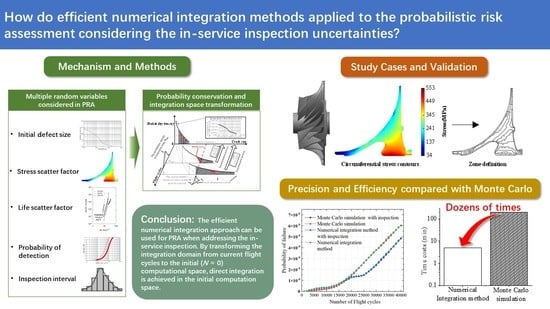
Theoretically, the numerical integration algorithm and Monte Carlo simulation should be entirely equivalent in terms of calculation results. In other words, the Monte Carlo simulation result would converge to that of the numerical integration algorithm if the sample size were sufficiently large. However, a slight discrepancy in the failure probability before 15,000 flight cycles is observed between the two methods, as shown in Figure 13. This diversity is related to the numerical algorithms and will be further probed in subsequent studies. However, this diversity has no notable impact on this study’s conclusions because the probability of failure before 15,000 flight cycles is relatively low.

Table 3. Probability of failure at 40,000 flight cycles for different methods.

Calculation Method	Probability of Failure at 40,000 Flight Cycles	Relative Error
Monte Carlo simulation with inspection	4.8741197 × 10−9	-
Monte Carlo simulation without inspection	6.0264085 × 10−9	-
Numerical integration with inspection	4.8309859 × 10−9	0.8%
Numerical integration without inspection	6.0202465 × 10−9	0.1%

presents the calculation results at 40,000 flight cycles. A maximum relative error of 5% exists at 10,000 flight cycles between the numerical integration algorithm and the Monte Carlo simulation.

With five random variables considered, the NI method exhibits a higher computational efficiency than MCS with the same accuracy. However, the high efficiency of the NI method is limited to the number of variables. It is well known that the computational efficiency of the MCS method is not affected by the number of variables, so it is suitable for calculating the failure probability of very high-dimensional variable space systems. However, the computational efficiency of the NI method decreases as the number of variables increases, and more research is needed for its use in the computation of failure risk of high-dimensional stochastic dynamical systems.

4. Conclusions

This study proposes an efficient numerical integration algorithm to consider in-service inspection in calculating the probability of failure. The integration formula of failure probability is deduced. The flowchart is established for the proposed method. Moreover, a centrifugal compressor disk model is applied. The corresponding results are compared with those of a Monte Carlo simulation to analyze the precision and efficiency of this algorithm. The following conclusions are obtained.

The efficient numerical integration approach can be used for PRA when addressing the in-service inspection. Through the transformation of the integration domain from current flight cycles to the initial (N = 0) computational space, direct integration is achieved in the initial computation space. The implementation of this algorithm solves the limitation of the Monte Carlo simulation for large numbers of samples.

The proposed algorithm has a calculation efficiency that is dozens of times better than the Monte Carlo simulation under a maximum relative error of 5%. This method provides engine component designers with a powerful tool for analyzing design safety. Further studies need to consider restricting the variables’ number using the proposed method.

With the continuous improvement of advanced engine performance, the development of new materials, and the emergence of new application scenarios, the requirements for the computational accuracy and computational efficiency of probabilistic failure risk assessment techniques are increasing. Future probabilistic algorithms should be developed to address the following aspects: transient, systematic, and full life cycle analysis. Firstly, the probabilistic risk assessment should describe the damage evolution under the transient thermal–mechanical coupling loads of advanced aero-engine rotors. Secondly, to systematically evaluate the complex damage evolution mechanism under multiple characteristic parts, multiple damage types and failure modes, the probabilistic algorithm needs to solve the contradiction between the stochastic calculation efficiency, the number of random variables, and the calculation accuracy. Finally, a probabilistic algorithm for the integration of material–manufacturing–design–operation failure risk needs to be constructed to apply the whole life cycle digital twin technology to risk analysis of rotors with limited life.

References

1. Mcclung, R.C.; Lee, Y.D.; Enright, M.P.; Liang, W. New Methods for Automated Fatigue Crack Growth and Reliability Analysis. In ASME Turbo Expo 2012: Turbine Technical Conference and Exposition; American Society of Mechanical Engineers: New York, NY, USA, 2012. [Google Scholar]
2. Chamis, C.C. Damage Tolerance and Reliability of Turbine Engine Components: National Aeronautics and Space Administration; Glenn Research Center: Cleveland, OH, USA, 1999. [Google Scholar]
3. Lin, K.Y.; Styuart, A.V. Probabilistic approach to damage tolerance design of aircraft composite structures. J. Aircr. 2007, 44, 1309–1317. [Google Scholar] [CrossRef]
4. Wu, Y.T.; Enright, M.P.; Millwater, H.R. Probabilistic methods for design assessment of reliability with inspection. AIAA J. 2002, 40, 937–946. [Google Scholar] [CrossRef]
5. Federal Aviation Administration. Advisory Circular 33.70-1. Guidance Material for Aircraft Engine-Life-Limited Parts Requirements; U.S. Department of Transportation, FAA: Washington, DC, USA, 2009.
6. Federal Aviation Administration. Advisory Circular 33.70-2. Damage Tolerance of Hole Features in High-Energy Turbine Engine Rotors; U.S. Department of Transportation, FAA: Washington, DC, USA, 2009.
7. Federal Aviation Administration. Advisory Circular 33.14-1. Damage Tolerance for High Energy Turbine Engine Rotors; U.S. Department of Transportation, FAA: Washington, DC, USA, 2001.
8. Abdessalem, A.B.; El-Hami, A. A probabilistic approach for optimising hydroformed structures using local surrogate models to control failures. Int. J. Mech. Sci. 2015, 96–97, 143–162. [Google Scholar] [CrossRef]
9. Enright, M.P.; Hudak, S.J.; McClung, R.C.; Millwater, H.R. Application of Probabilistic Fracture Mechanics to Prognosis of Aircraft Engine Components. AIAA J. 2006, 44, 311–316. [Google Scholar] [CrossRef]
10. Huyse, L.; Enright, M.P. Efficient conditional failure analysis: Application to an aircraft engine component. Struct. Infrastruct. Eng. 2006, 2, 221–230. [Google Scholar] [CrossRef]
11. Enright, M.P.; McClung, R.C.; Sobotka, J.C.; Irving, G.; Joe, G. Influences of non-destructive inspection simulation on fracture risk assessment of additively manufactured turbine engine components. Turbo Expo: Power for Land, Sea, and Air. Am. Soc. Mech. Eng. 2018, 51135, V07AT32A013. [Google Scholar]
12. Gorelik, M. Additive manufacturing in the context of structural integrity. Int. J. Fatigue 2017, 94, 168–177. [Google Scholar] [CrossRef]
13. Enright, M.P.; Millwater, H.R.; Huyse, L. Adaptive Optimal Sampling Methodology for Reliability Prediction of Series Systems. AIAA J. 2006, 44, 523–528. [Google Scholar] [CrossRef]
14. Millwater, H.R.; Enright, M.P.; Fitch, S.H.K. Convergent Zone-Refinement Method for Risk Assessment of Gas Turbine Disks Subject to Low-Frequency Metallurgical Defects. ASME J. Eng. Gas Turbines Power 2006, 129, 827–835. [Google Scholar] [CrossRef]
15. Wu, Y.T. Computational methods for efficient structural reliability and reliability sensitivity analysis. AIAA J. 1994, 32, 1717–1723. [Google Scholar] [CrossRef]
16. Kibria, A.; Castillo−Villar, K.K.; Millwater, H.R. Minimizing the discrepancy between simulated and historical failures in turbine engines: A simulation-based optimization method. Math. Probl. Eng. 2015, 2015, 813565. [Google Scholar] [CrossRef] [Green Version]
17. Yang, L.; Ding, S.T.; Wang, Z.Y.; Li, G. Efficient probabilistic risk assessment for aeroengine turbine disks using probability density evolution. AIAA J. 2017, 55, 2755–2761. [Google Scholar] [CrossRef]
18. Liu, J.B.; Ding, S.T.; Li, G. Influence of Random Variable Dimension on the Fast Numerical Integration Method of Aero Engine Rotor Disk Failure Risk Analysis. In ASME International Mechanical Engineering Congress and Exposition; American Society of Mechanical Engineers: New York, NY, USA, 2020; Volume 84669. [Google Scholar]
19. Kozin, F. On the Probability Densities of the Output of Some Random Systems. J. Appl. Mech. 1961, 28, 161–164. [Google Scholar] [CrossRef]
20. Christian, A.; Kadau, K. Numerically efficient modified Runge–Kutta solver for fatigue crack growth analysis. Eng. Fract. Mech. 2016, 161, 55–62. [Google Scholar]
21. L’Ecuyer, P.; Simard, R.; Chen, E.J.; Kelton, W.D. An Object-Oriented Random-Number Package with Many Long Streams and Substreams. Oper. Res. 2002, 50, 1073–1075. [Google Scholar] [CrossRef]
22. Enright, M.P.; Huyse, L. Methodology for Probabilistic Life Prediction of Multiple-Anomaly Materials. AIAA J. 2006, 44, 787–793. [Google Scholar] [CrossRef]
23. Pan, X.; Ding, S.; Zhang, W.; Liu, T.; Wang, L.; Wang, L. Probabilistic Risk Assessment in Space Launches Using Bayesian Network with Fuzzy Method. Aerospace 2022, 9, 311. [Google Scholar] [CrossRef]
24. Xu, T.; Ding, S.; Zhou, H.; Li, G. Machine learning-based efficient stress intensity factor calculation for aeroengine disk probabilistic risk assessment under polynomial stress fields. Fatigue Fract. Eng. Mater. Struct. 2021, 45, 451–465. [Google Scholar] [CrossRef]
25. Li, J.; Chen, J.B. Advances in the research on probability density evolution equations of stochastic dynamical systems. Adv. Mech. 2010, 40, 170–188. [Google Scholar]
26. Li, J.; Chen, J.B. The principle of preservation of probability and the generalized density evolution equation. Struct. Saf. 2008, 30, 65–77. [Google Scholar] [CrossRef]
27. Sub-Team to the Aerospace Industries Association Rotor Integrity Sub-Committee. The development of anomaly distributions for aircraft engine titanium disk alloys. In Proceedings of the 38th Structures, Structural Dynamics, and Materials Conference, Kissimmee, FL, USA, 7–10 April 1997. Paper No: AIAA 97-1068. [Google Scholar]
28. Newman, J.C.; Raju, I.S. Stress-intensity factor equations for cracks in three-dimensional finite bodies. In Fracture Mechanics: Fourteenth Symposium—Volume I: Theory and Analysis; ASTM International: West Conshohocken, PA, USA, 1983; pp. 238–265. [Google Scholar]
29. Glinka, G.; Shen, G. Universal features of weight functions for cracks in mode I. Eng. Fract. Mech. 1991, 40, 1135–1146. [Google Scholar] [CrossRef]
30. Zhou, H.M.; Ding, S.T.; Guo, L. Universal weight function method on the probabilistic surface damage tolerance assessment of aeroengine rotors. In ASME International Mechanical Engineering Congress and Exposition; American Society of Mechanical Engineers: New York, NY, USA, 2020; Volume 84669, p. V014T14A028. [Google Scholar]
31. Wang, L.; Wang, X.; Su, H.; Lin., G. Reliability estimation of fatigue crack growth prediction via limited measured data. Int. J. Mech. Sci. 2017, 121, 44–57. [Google Scholar] [CrossRef]
32. Paris, P.; Erdogan, F. A critical analysis of crack propagation laws. J. Basic Eng. 1963, 85, 528–533. [Google Scholar] [CrossRef]
33. Anderson, T.L. Fracture Mechanics: Fundamentals and Applications; CRC Press: Boca Raton, FL, USA, 2017. [Google Scholar]
34. Wehling, P.; LaBudde, R.A.; Brunelle, S.L.; Nelson, M.T. Probability of detection (POD) as a statistical model for the validation of qualitative methods. J. AOAC Int. 2011, 94, 335–347. [Google Scholar] [CrossRef]
35. Ding, S.T.; Wang, Z.Y.; Qiu, T.; Zhang, G.; Li, G. Probabilistic failure risk assessment for aeroengine disks considering a transient process. Aerosp. Sci. Technol. 2018, 78, 696–707. [Google Scholar] [CrossRef]
36. Enright, M.P.; McFarland, J.; McClung, R.; Wu, W.T.; Shankar, R. Probabilistic Integration of Material Process Modeling and Fracture Risk Assessment Using Gaussian Process Models. In Proceedings of the 54th AIAA/ASME/ASCE/AHS/ASC Structures, Structural Dynamics, and Materials Conference, Boston, MA, USA, 8–11 April 2013. [Google Scholar]
Figure 1. Schematic diagram of the stochastic dynamic system for risk assessment.
Aerospace 09 00525 g001
Figure 2. Initial defect distribution curve of hard α defects [7].
Aerospace 09 00525 g002
Figure 3. Schematic diagram of probability space transformation under single variable.
Aerospace 09 00525 g003
Figure 4. Schematic diagram of probability space transformation under multi variables.
Aerospace 09 00525 g004
Figure 5. Probability of detection curve of ultrasonic [7].
Aerospace 09 00525 g005
Figure 6. Detection domain through POD.
Aerospace 09 00525 g006
Figure 7. Detection domain through POD and inspection time.
Aerospace 09 00525 g007
Figure 8. Schematic diagram of failure probability risk evolution process with in-service inspection.
Aerospace 09 00525 g008
Figure 9. Flowchart of the presented efficient numerical integration algorithm for risk assessment considering in-service inspection.
Aerospace 09 00525 g009
Figure 10. Geometry, finite element model, and the quadrilateral mesh of the compressor disk.
Aerospace 09 00525 g010
Figure 11. Stress contours and zone definition: (a) Circumferential stress contours; (b) Zone definition.
Aerospace 09 00525 g011
Figure 12. Comparison of the time costs of different methods.
Aerospace 09 00525 g012
Figure 13. Comparison of the probability of failure of different methods.
Aerospace 09 00525 g013