1. Introduction
Gravitational-wave detection has become increasingly attractive following the first direct observation made by the Laser Interferometer Gravitational-Wave Observatory (LIGO) [
1,
2,
3,
4]. The signatures of a gravitational-wave can be detected using a laser interferometer [
5,
6,
7,
8]. However, due to the limitation of the Earth’s curvature and vibration, it is difficult to detect (e.g., LIGO) gravitational-waves with a frequency of lower than 10 Hz [
9,
10,
11,
12,
13]. Compared with the ground-based observatory, space-based gravitational-wave observatories have much longer arm lengths and are free from the noise related to the seismic and gravity gradient [
14,
15,
16]. Therefore, space-based gravitational-wave observatories are much more sensitive to low-frequency gravitational-waves, towards which interest and attention have recently been directed [
17].
Many space-based gravitational-wave observatories are currently in the development phase of research, such as with the Laser Interferometer Space Antenna (LISA/ eLISA) [
5,
9,
18,
19], TianQin [
12,
14,
20,
21], and TAIJI [
13,
22,
23,
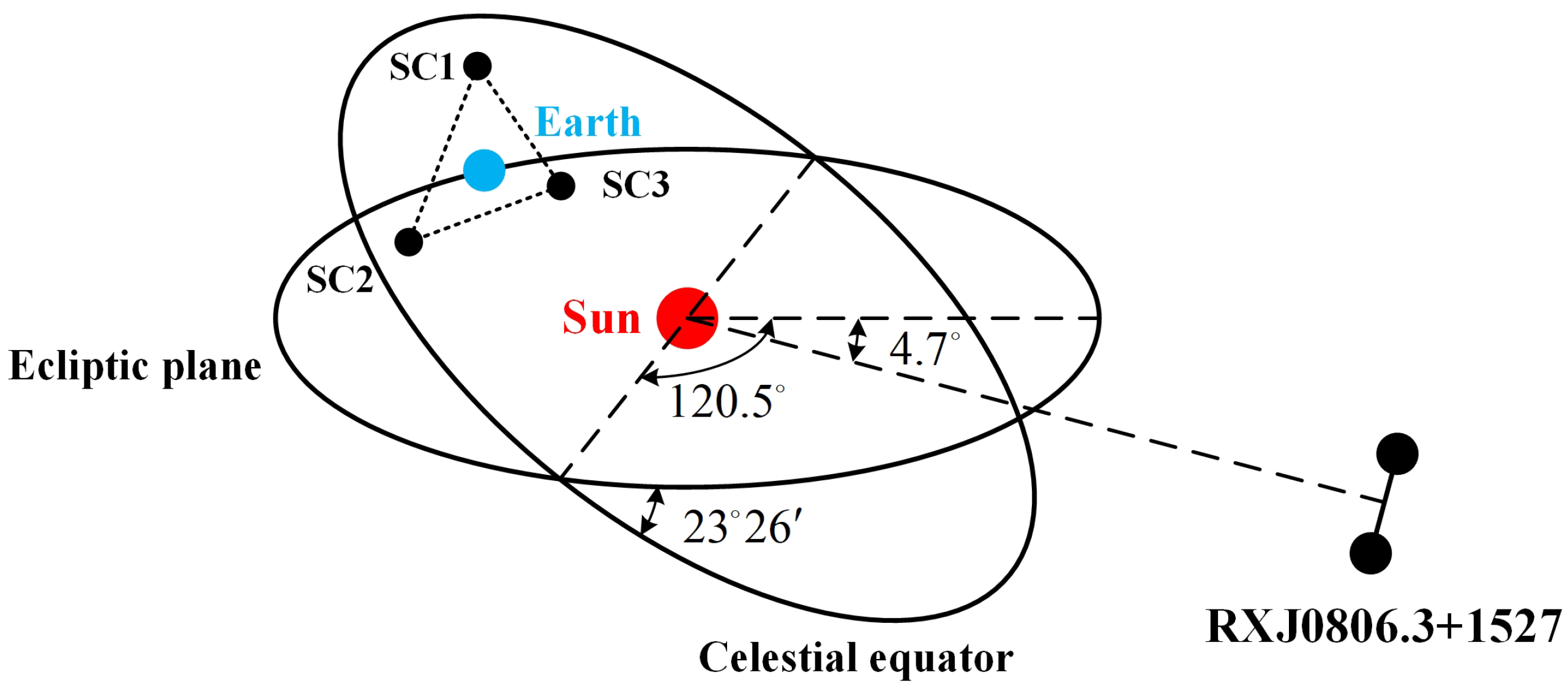
24]. In these planned space-based gravitational-wave observatories, three spacecraft are used; therefore, a triangular configuration is formed. Any one of the three spacecraft can be chosen as the center of the interferometer, while the other two become the endpoints of the two interferometer baselines. The LISA and the TAIJI projects are classic heliocentric designs, with three spacecraft orbiting the Sun [
13]. TianQin is another space-based gravitational-wave observatory project put forward by the Sun Yat-sen University in 2016 [
12]. Different from the LISA/eLISA and TAIJI projects, the TianQin project is a geocentric gravitational-wave observatory. The TianQin project is a constellation containing three identical drag-free controlled detectors in high Earth orbits with an altitude of
km [
7].
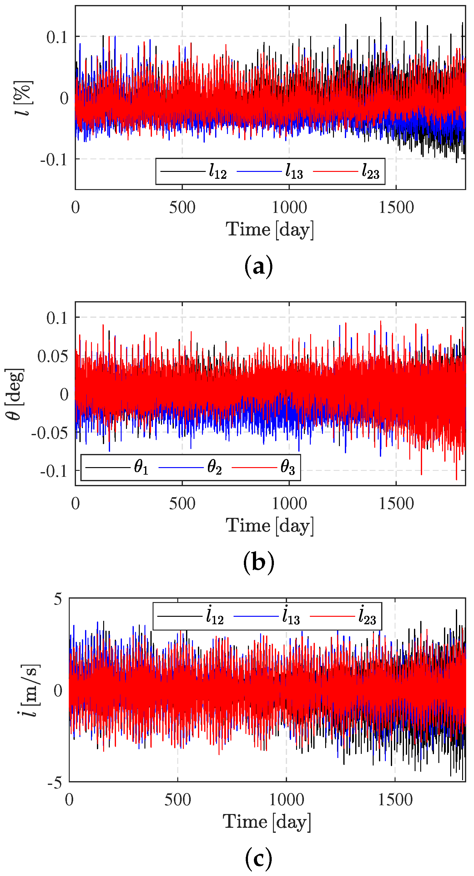
For these mentioned space-based gravitational-wave observatories, long-term configuration stability is usually required to guarantee the performance of interferometric detection. The configuration stability of the space-based gravitational-wave observatories can be measured with three configuration parameters: the arm length, the breathing angle and the relative velocity [
24]. The changes in configuration parameters will result in Doppler shift in the laser signals and the beam pointing variations, exceeding the capacity of the detection payloads [
7]. The permitted changes in these stability indexes are determined according to the capacity of the scientific payloads, and are taken into consideration when designing and optimizing the orbits. Although the pre-designed and optimized nominal orbits can meet the configuration stability requirements, the long-term behavior of the configuration may still be hazardous due to multiple factors, in which the insertion errors are the most significant ones. Affected by the insertion errors, the spacecraft will deviate from their nominal orbits, and in turn, the long-term stability requirements are no longer satisfied [
12,
13,
25]. Therefore, it is necessary to investigate the configuration uncertainty propagation problems and analyze the influence of the insertion errors on the configuration stability.
Generally, uncertainty propagation is used to characterize the variable’s moment (usually represented by mean and covariance matrix) or probability density function (PDF) [
26,
27,
28,
29,
30]. Various uncertainty propagation methods have been proposed, including Monte Carlo simulations [
31,
32], the Linear Covariance Analysis (LinCov) [
33], the Covariance Analysis Description Equation Technique (CADET) [
34], Unscented Transformation (UT) and its variants [
35,
36,
37], Polynomial Chaos (PC) [
38,
39,
40], and State Transition Tensors (STT) and its variants [
41,
42,
43]. These approaches have been well investigated to solve the uncertainty propagation problem in orbital mechanics for a single spacecraft [
26,
44,
45,
46]. Few works focus on the uncertainty propagation problem of a constellation configuration. Li et al. investigated the stability of the heliocentric gravitational detection observatory using the CADET and the UT methods, and some properties were found [
13]. The heliocentric gravitational detection observatory is inherently a formation in the heliocentric inertial coordinate, and the motions of the spacecraft can be fully described using the relative dynamic equation. Compared with heliocentric gravitational detection observatories, the geocentric gravitational detection observatory orbits around the Earth, and is classified as the constellation. Therefore, the dynamic environment of the geocentric gravitational detection observatory is different from that of the heliocentric ones, which makes stability properties different. Thus, it is necessary to perform the stability analysis of the geocentric gravitational-wave observatory, and uncover the effects of the insertion errors on the stability of the geocentric gravitational-wave observatory.
This paper focuses on investigating the stability of the geocentric gravitational-wave observatory. The TianQin project is selected as the research object in this paper. The stability domain of the geocentric gravitational-wave observatory is analyzed from the view of the configuration uncertainty propagation. The effects of the insertion errors on the configuration stability are investigated based on the UT method. The accuracy of the UT methods with different UT tuning factors is discussed via a comparison with the Monte Carlo (MC) simulations, and the best UT tuning factors for addressing the configuration uncertainty propagation problem is selected. The effects of the insertion errors in different directions and with different magnitudes are studied. Furthermore, the stability domain, in which the stability requirements are always met, is determined and analyzed. Compared with the configuration uncertainty propagation analysis of the heliocentric designs, some more interesting conclusions are found.
The remainder of this paper is organized as follows.
Section 2 begins by describing the configuration design and the dynamic model of the geocentric gravitational-wave observatory. The three stability indexes, i.e., the arm length, the breathing angle and the relative velocity, are presented.
Section 3 begins by briefly describing the UT method, followed by an accuracy analysis of the UT method with different UT tuning factors. The effects of the insertion errors in different spatial directions are considered. The stability domain of the geocentric space gravitational detection constellation is computed and analyzed in
Section 4. Finally, the conclusions are provided in
Section 5.
3. Configuration Uncertainty Propagation Based on UT Method
This section begins with a brief review of the UT method, followed by the accuracy of the UT method using different tuning factors which are analyzed in
Section 3.2. The best UT tuning factors are determined. Finally, the characteristics of the configuration uncertainty propagation of the geocentric gravitational-wave observatory is analyzed based on the UT method.
3.1. Unscented Transformation Method
According to Equations (
1)–(
4), the transformation from the orbit insertion state
to the stability indexes
is nonlinear, which has two distinctive features. The first is that this transformation is a black-box model, which has no analytical solutions. Therefore, analytical uncertainty propagation methods, such as the CADET or STT, are not appropriate for solving the configuration uncertainty propagation. The second feature is that the calculation of this transformation is an expensive process as long-term numerical integration is required.
The sigma-point based methods allow for the use of already existing propagation tools as a black-box and avoids any analytical solutions or gradient information, which can be conveniently extended to solve the configuration problem. The widely used sigma-point methods include the UT method, Conjugate Unscented Transform (CUT) and Cubature rules (CRs). These sigma-point methods approximate the probability distribution at a future time by nonlinearly integrating a few sigma-samples, which are deterministically selected according to the given initial distribution. Among these sigma-point methods, the UT method has less computational overhead and has been successfully applied to solve the configuration uncertainty propagation problem of a heliocentric gravitational-wave observatory (the TAIJI project). Thus, considering the factors of time, cost and convenience, the UT is used in this paper.
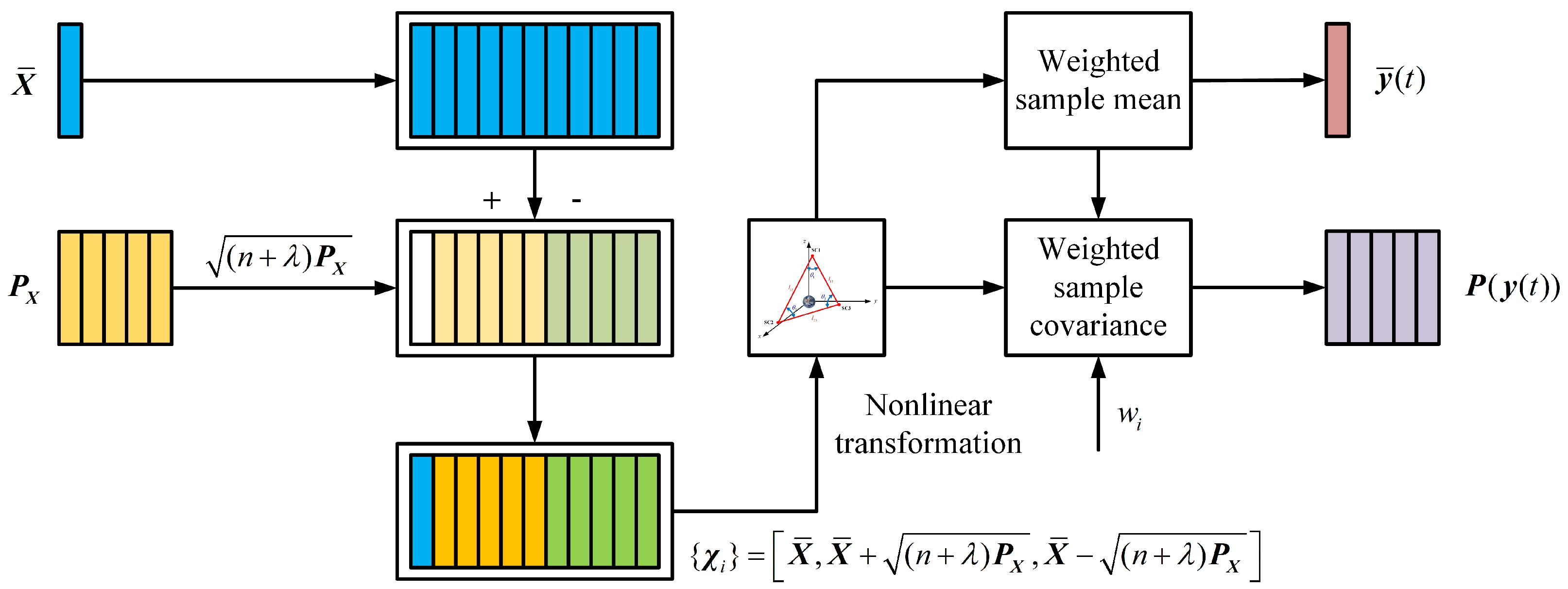
The schematic diagram of the UT method is illustrated in
Figure 5. Consider the random variable
with the mean
and covariance
as follows:
According to the mean
and covariance
, the sigma-point set
is then formulated as:
where
is the dimension of the variable
;
denotes the
i-th column of the matrix;
is an adjusting dispersion parameter called the UT tuning factor; and
can be obtained using the Cholesky decomposition, which satisfies
.
The weights of the
i-th sigma points
are obtained as follows:
For each orbit insertion state
, the orbits of the three spacecraft are propagated using the RungeKutta45 method; then, the corresponding stability indexes
are obtained according to Equations (
2)–(
4). According to the UT method, the mean
and covariance matrix
of the stability indexes are approximated by
According to the equations above, the distributions of the stability indexes of any time in the mission lifetime can be obtained by calculating 37 sigma points.
3.2. Selection of the UT Tuning Factor
In this subsection, the accuracy of the UT method is analyzed. To use the UT method, the UT tuning factor
should be carefully selected. In [
13], the value of
is selected as
, for which the selection followed from the recommendation in Julier and Uhlmann that
[
35]. In this case, the kurtosis of one state of the sigma points agrees with that of the Gaussian distribution. However, for high-dimensional problems such as the configuration uncertainty propagation, this value produces a negative weight at the mean, which may adversely affect the performance of the UT. Therefore, it is worth testing the UT methods with different tuning factors and comparing the performances.
For simplicity,
denotes the variable related to the UT tuning factor. A total of nine UT methods are tested, with the variable
. Two cases, including a standard case and a severe case, are simulated to verify the performance of the UT methods with different tuning factors. The standard deviation (STD) of the insertion errors of the two cases are listed in
Table 3. The covariance matrix of the insertion errors of the standard case is written as:
where
denotes the 3-dimensional identified matrix.
According to
Table 3, for the severe case, the covariance matrix of the insertion errors is partitioned as:
The results predicted by the UT methods are compared with the Monte Carlo simulation method. The number of the samples used in the Monte Carlo simulation is set to 1000. Taken the covariance predicted by the Monte Carlo simulation as a standard, the relative error of the covariance obtained by the UT methods is defined as:
where
is the defined relative errors of two matrices;
and
are the covariance matrices calculated by the Monte Carlo simulation and UT methods at the epoch
t, respectively; and
represents the Frobenius norm (sum square of the elements). The smaller the
, the better the performance.
The relative errors
of the UT methods using different tuning factors are computed. For each UT tuning factor, the relative errors at 11 epochs are tested. The testing epochs begin at 0 and end at 5 years, with a time interval of 0.5 years. The average relative errors of the 11 epochs of different UT methods are listed in
Table 4. For the standard case, the nine UT methods possess a similar performance. However, for the severe case, the performances of the nine UT methods differ. For example, the relative error of the UT method
is around 0.1103, while for the UT method
, the relative error is around 0.2188. To better compare the performance of different UT methods in predicting the covariance of the three stability indexes, a weighted index is proposed by combing the relative errors of the arm length, the breathing angle and the relative velocity as follows:
where
denotes the weighted relative error. The values of the weighted relative errors of different UT methods are also listed in
Table 4. The UT method with a tuning factor
of equal to −9 (
) has the smallest relative errors; therefore, in this paper,
is selected as the UT tuning factor for the following analysis.
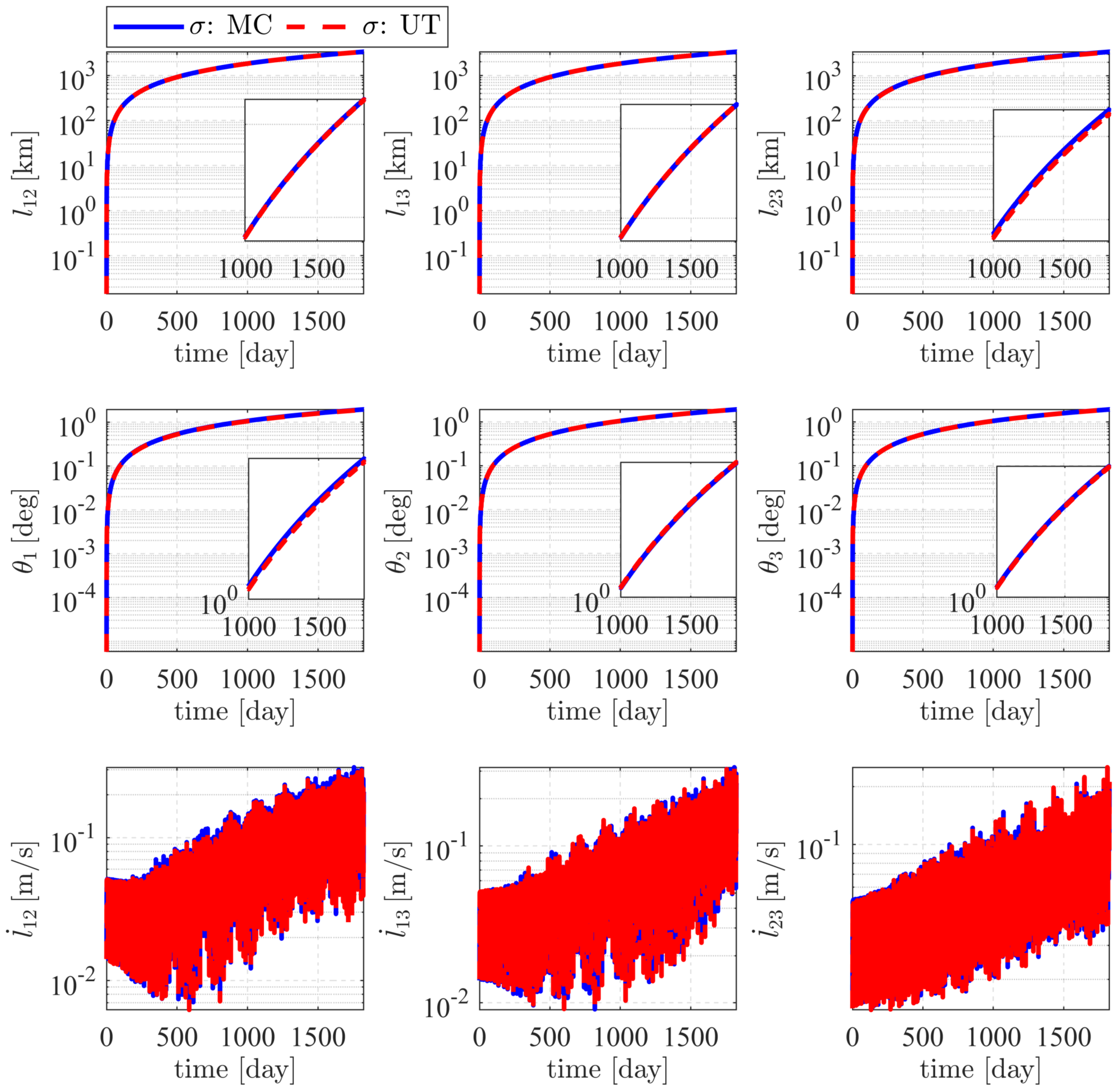
Figure 6 shows the STD results of the standard case obtained by the UT method (
), and the results are compared with those obtained by the Monte Carlo simulation (1000 samples). The blue lines represent the results of Monte Carlo and the red dashed lines represent the results obtained by the UT. Moreover, the predicted stability indexes’ uncertainties at epoch
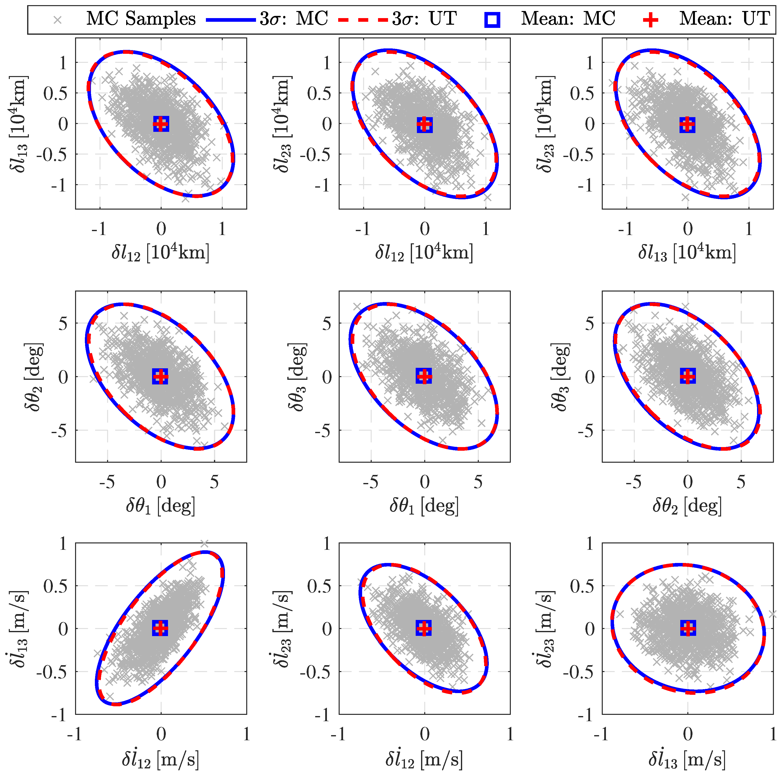
years, are illustrated in
Figure 7. The corresponding means and the 3
ellipsoid bounds are projected. In addition, for the sake of comparison, 1000 Monte Carlo samples are plotted the grey ‘x’. The mean and the 3
ellipsoid bounds obtained by the Monte Carlo simulation are shown by the blue squares and blue dashed lines. It can be seen that the UT method can accurately represent the curvature exhibited by the Monte Carlo samples and the predicted 3
bounds are very close to that of the Monte Carlo simulation. The STDs of the three stability indexes at the epoch
year predicted by the UT and Monte Carlo simulation are shown in
Table 5. It can be found that compared with the Monte Carlo simulation, the UT can predict the STDs with errors of no more than 2.7%.
The simulations were performed using MATLAB R2018b on a computer with a 3.6 GHz AMD Ryzen processor and 16 GB RAM. As shown in
Table 6, with the 1000 samples (including 3000 orbits) made for the Monte Carlo simulation, it takes about 9728.3374 s (around 2.7 h). However, the computational time of the UT method is only 347.2791 s (around 5.8 min), which is only 3.5697% that of the Monte Carlo simulations.
3.3. Configuration Uncertainty Propagation Analysis for the Geocentric Space Gravitational Wave Detection Constellation
The effects of the insertion errors in different directions are investigated using the UT method. For an uncertainty variable
, given a certain direction
and the standard deviation
, the corresponding covariance matrix of
is written as:
The radial, tangential and normal position and velocity insertion errors are considered. For radial position and velocity uncertainty, the covariance matrices are obtained as follows:
For tangential position and velocity uncertainty:
Additionally, for normal position and velocity uncertainty:
where
and
represent the STD of the position and velocity insertion errors, respectively.
Note that to use the UT method, Cholesky decomposition is required to calculate the matrix
. To avoid numerical singularity, an identified matrix with tiny values is added to the matrix
. For example, for the condition that only radial position insertion errors exist, the covariance matrix
is obtained as follows:
where
is an 18-dimensional identified matrix.
First, the configuration stability considering only the insertion errors of spacecraft 1 is investigated. When we consider the effects of the position insertion errors of spacecraft 1 in different directions, only three variables are included, which can be plotted using a three-dimensional figure.
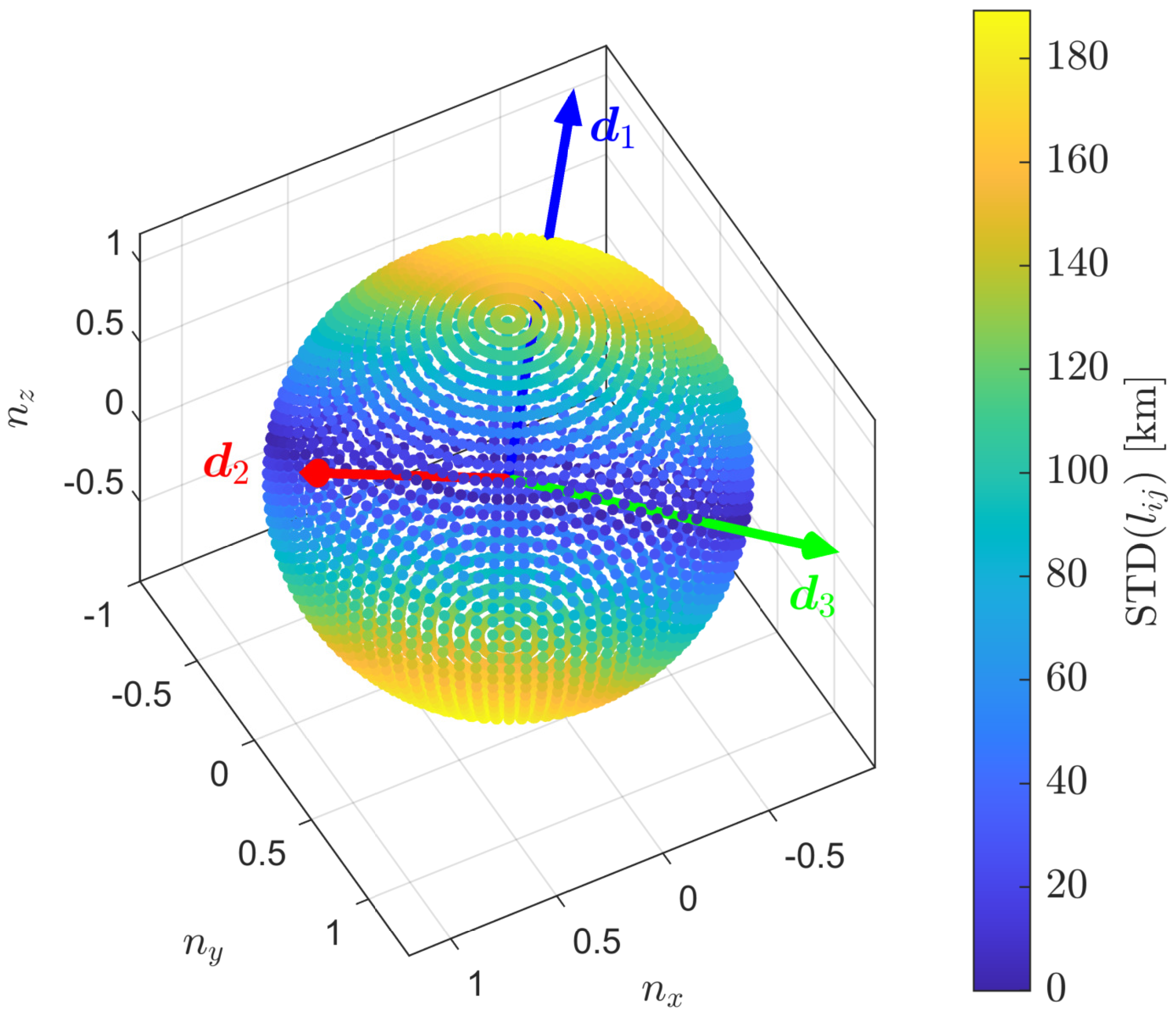
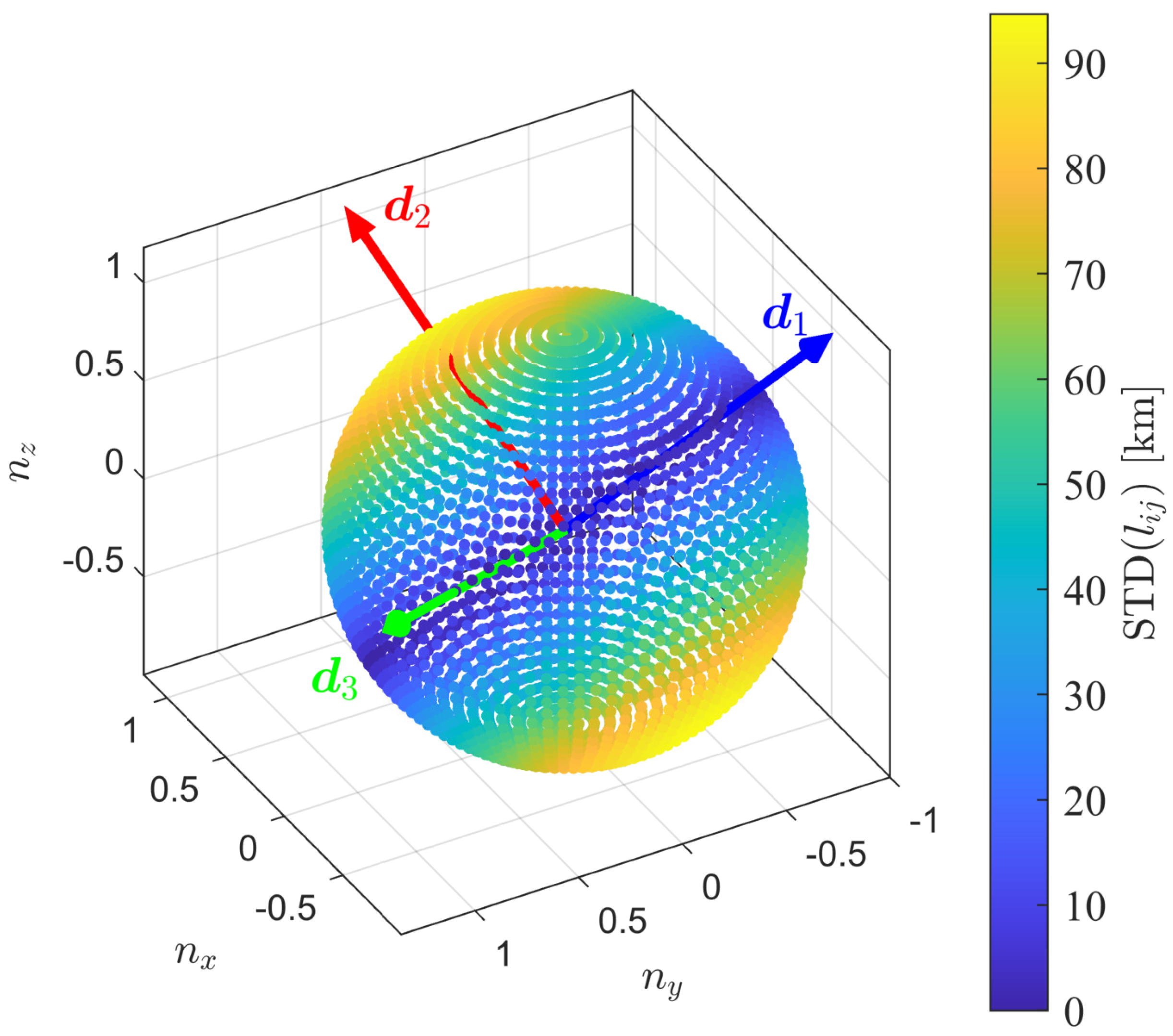
The effects of the position and velocity insertion errors on the stability indexes are studied independently. Assume that the STD of the position and velocity insertion error are 100 m and 0.001 m/s, respectively. A myriad of directions are generated, and for each direction, configuration uncertainty propagation is performed based on the UT method. The results are shown in
Figure 8 and
Figure 9. In
Figure 8 and
Figure 9,
denotes the direction of the insertion errors and each point on the united sphere denotes a spatial direction, and the predicted STD of the arm length is represented by the color. For better comparison, the radial, the tangential and the normal directions are labeled by the blue (
), red (
) and green (
) lines, respectively, in
Figure 8 and
Figure 9. It can be seen that the effects of the radial position insertion errors and the tangential velocity insertion errors are much more significant than the insertion errors in other directions.
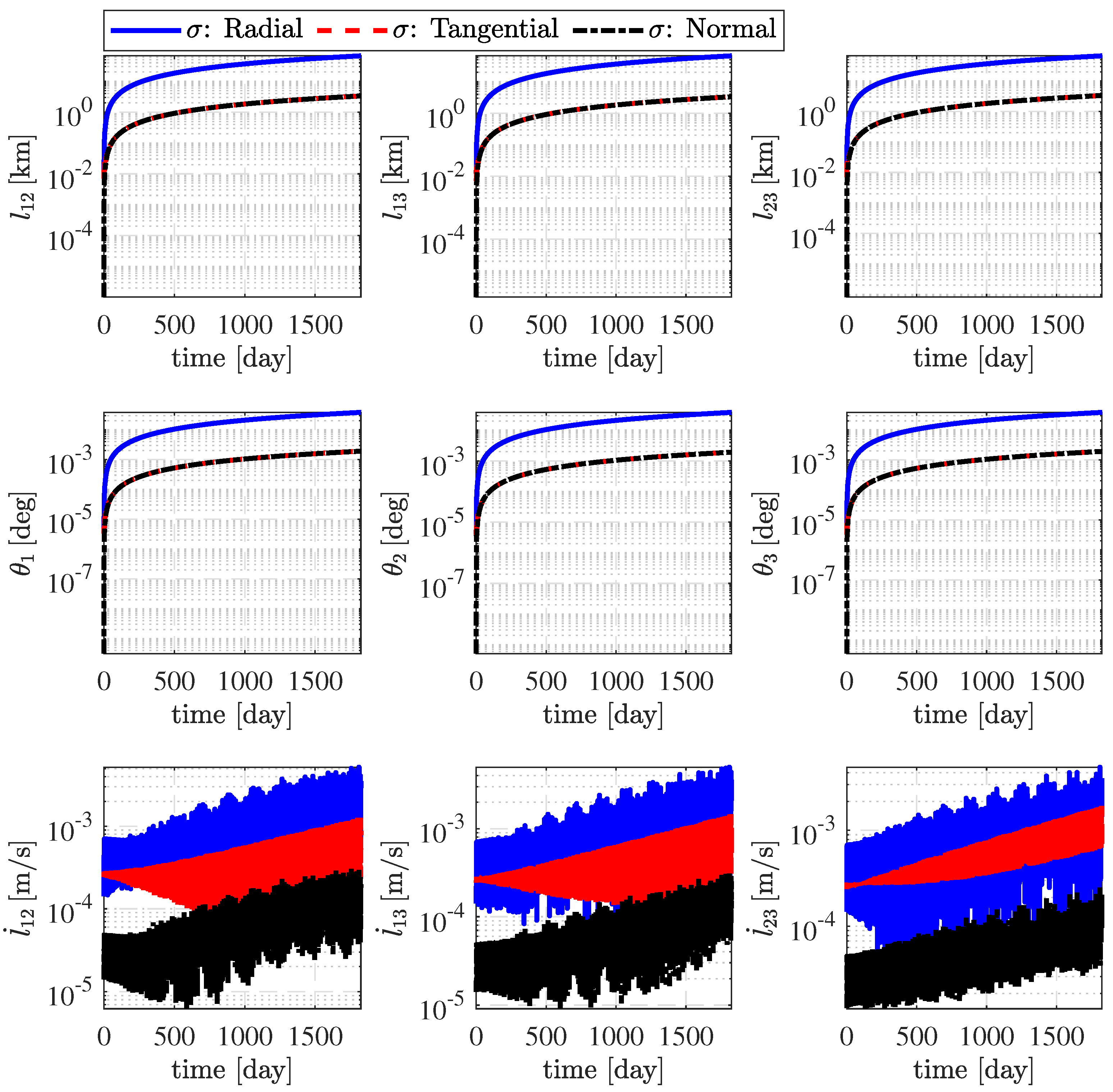
According to the parameter setting in the standard case in
Table 3, let
m and
mm/s. The effects of the radial, tangential and normal position insertion errors on the stability indexes are shown in
Figure 10 and
Table 7.
Figure 10 illustrates the time history of the STDs of the arm length, the breathing angle and the relative velocity considering only the position insertion errors.
Table 7 lists the STDs of the three stability indexes at the epoch year under the position insertion errors in different directions. It is found that the arm length and the breathing angle are mainly affected by the radial position insertion errors. The arm length STDs under radial position errors are around 66.8 km, which is about 20 times that under tangential and normal position insertion errors (around 3.34 km).Furthermore, the relative velocity is mainly affected by the radial position insertion errors, and is greatly influenced by the tangential position insertion errors. Among the three directions, the normal position insertion errors have the least effect on the three stability indexes.
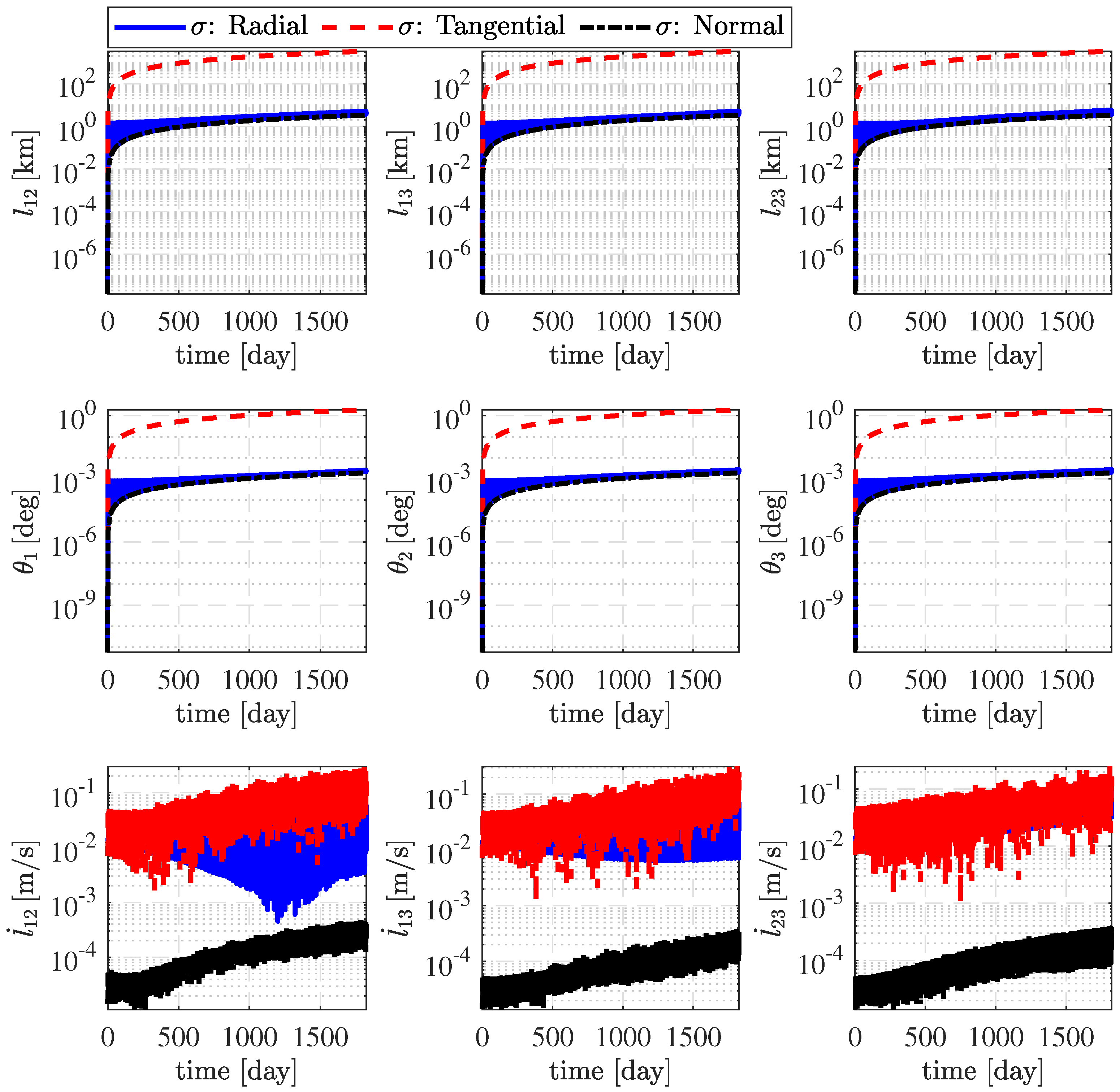
The effects of the radial, tangential and normal velocity insertion errors on the stability indexes are shown in
Figure 11 and
Table 8. It can be seen that the tangential velocity insertion errors have strong influences on the arm length, the breathing angle and the relative velocity. The normal velocity insertion errors have moderate effects on the relative velocity.
According to the above discussion, the effects of the position and velocity insertion errors in different directions are summarized as follows. The radial position insertion errors and the tangential velocity insertion errors strongly affect the three stability parameters. The tangential position insertion errors and radial velocity insertion errors only affect the relative velocity. Moreover, the normal insertion errors have almost no effect on the three stability parameters. The effects of the radial position insertion errors and the tangential velocity insertion errors can be explained as follows. The radial position and the tangential velocity deviation will directly affect the potential energy and kinetic energy of the spacecraft, which causes the orbital period of the spacecraft to be at variance with another spacecraft in the constellation. The phase difference between two spacecraft deviates in the long-term; as a result, the desired regular triangle configuration is impacted. In this case, the arm length and the breathing angle change considerably. However, the insertion errors in other directions only change the spacecraft’s orbital plane, which almost has no influence on the configuration.
4. Stability Domain Analysis for the Geocentric Space Gravitational Wave Detection Constellation
This section provides the stability domain analysis for the geocentric space gravitational-wave detection constellation. First, the stability domain is analyzed by considering the independent and identically distributed insertion errors in position and velocity. Moreover, following the studies on the effects of uncertainty in different directions in
Section 3.3, the stability domains with uncertainty in spatial directions are investigated.
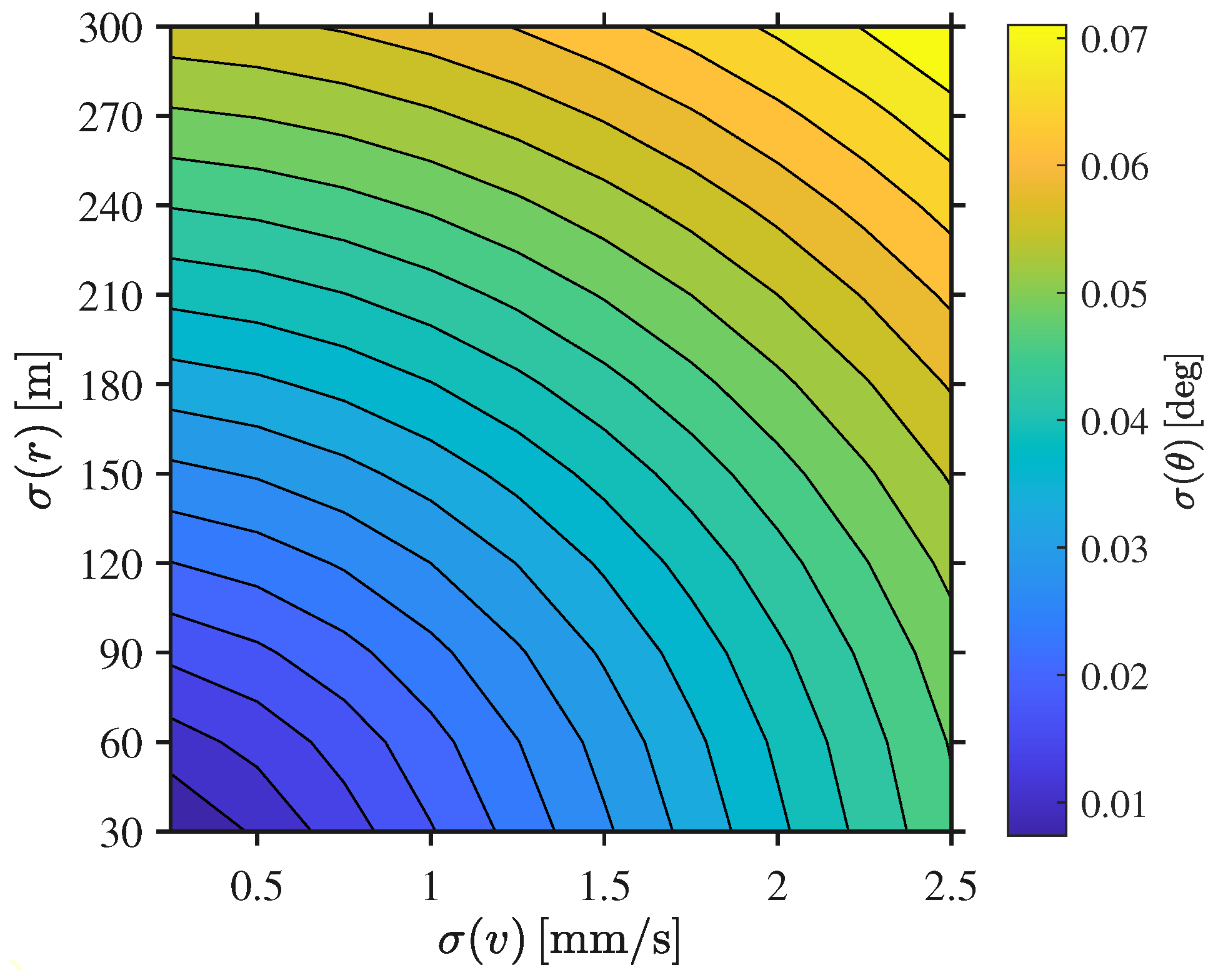
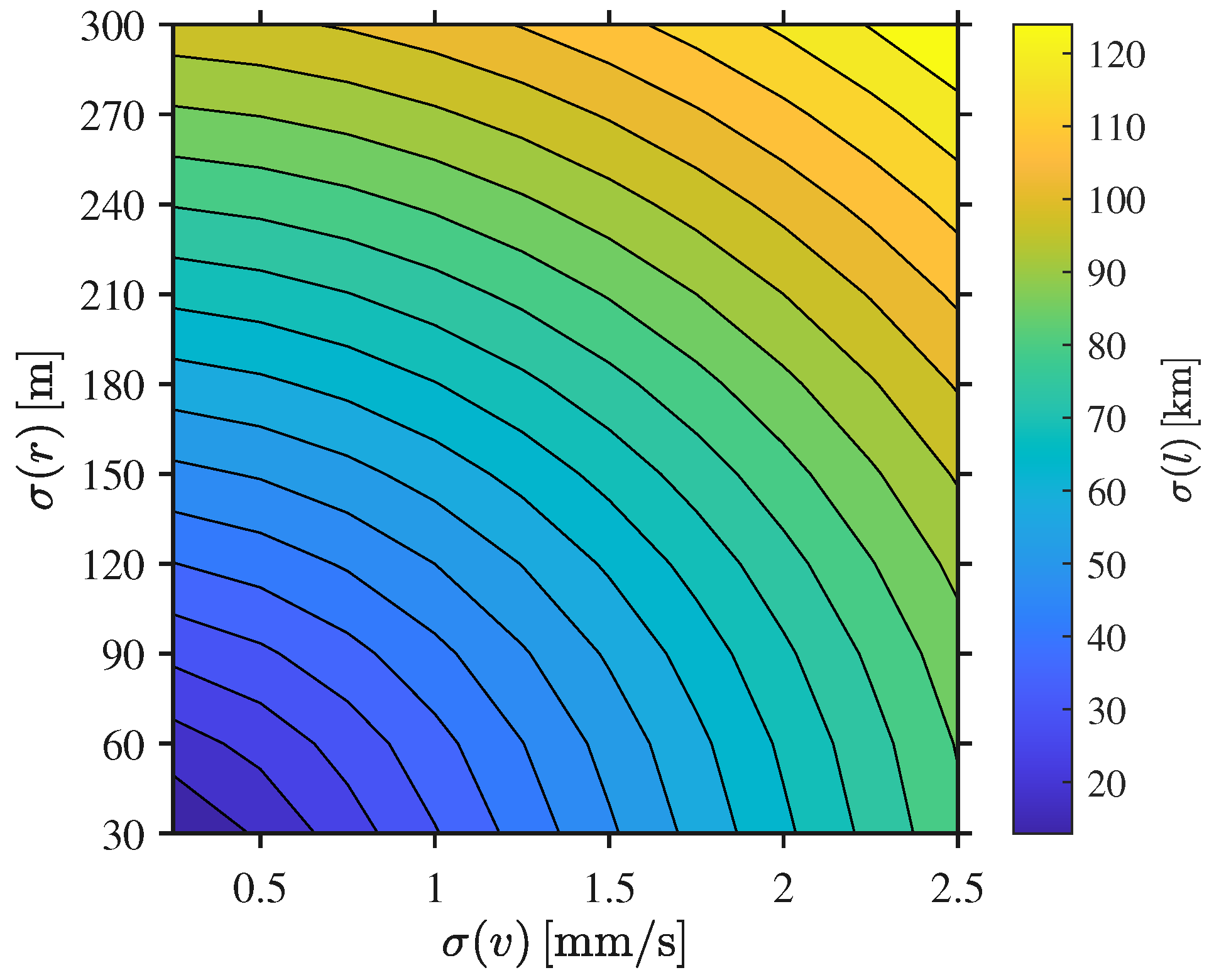
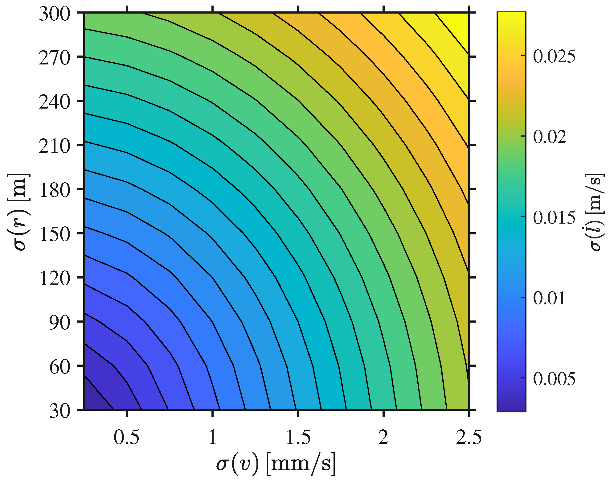
The independent and identically distributed insertion errors are firstly considered. For a case where the STD of the position insertion errors along three axes of the three spacecraft gradually increase from 30 m to 300 m, and the STD of the velocity insertion error increases from 0.5 mm/s to 5 mm/s, the maximal STDs of the arm length, the breathing angle and the relative velocity within three months are shown in
Figure 12,
Figure 13 and
Figure 14. For the case where the STD of the position insertion error equals 300 m and the STD of the velocity insertion error equals 5 mm/s, the maximal STDs of the arm length, the breathing angle and the relative velocity are 129.4790 km, 0.0742 deg and 0.0289 m/s, respectively. According to the permitted ranges of the three stability indexes listed in
Table 2, it is found that the breathing angle is most likely to exceed the stability constraint.
According to the predictions in
Figure 12,
Figure 13 and
Figure 14 and the stability constraints in
Table 2, the stability domain (inside the constraints) for a three-month propagation is determined and shown in
Table 9. For the three-month propagation, the insertions errors inside the constraints should satisfy the following equations:
The stability domains of the three-month propagation considering only radial insertion errors (i.e., the radial position insertion errors and the radial velocity insertion errors) were calculated; however, only tangential insertion errors and normal insertion errors are shown in
Table 9. It can be seen that when considering only radial insertion errors, if the position insertion errors exceed 340 m, or the velocity insertion errors exceed 600 mm/s, the three stability indexes will not meet the requirement in
Table 2. For the case of considering only tangential insertion errors, the permitted ranges of the position and velocity insertion errors are 40 km and 3 mm/s. Moreover, when considering only normal insertion errors, the permitted values of the position and velocity insertion errors are 140 km and 2.5 m/s, respectively. It was clearly found that the case of considering only normal insertion errors has the largest permitted ranges. As shown in
Table 7 and
Table 8, this is due to the findings that neither the normal position insertion error nor the normal velocity insertion error impart a strong influence on the configuration stability.
Furthermore, the maximal STDs of the arm length, the breathing angle and the relative velocity for a two-year mission lifetime under different insertion errors are also shown in
Table 9. It can be seen that, compared with the three-month case, the maximal position insertion error decreases from 340 to 21 m, and the maximal velocity insertion error decreases from 3 mm/s to 0.4 mm/s. The stability domains of the two-year case considering only radial insertion errors, tangential insertion errors and normal insertion errors are illustrated in
Table 9. For the two-year case considering only normal insertion errors, the position insertion errors should not exceed 45 km and the velocity insertion errors should not exceed 0.9 m/s.
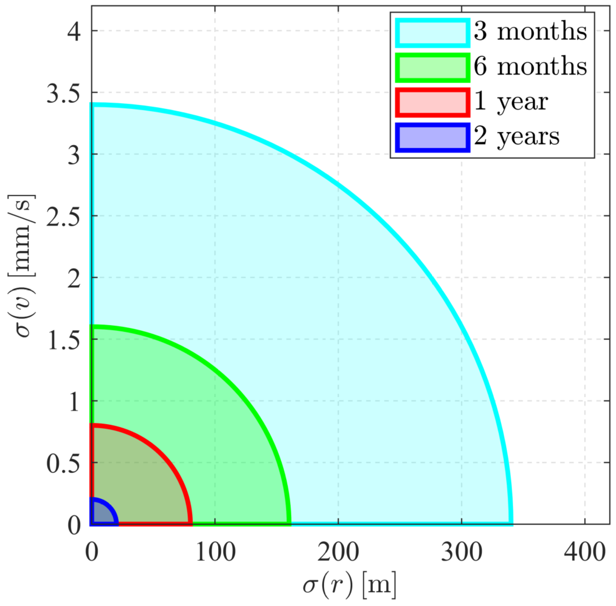
The stability domains of different mission lifetimes are shown in
Figure 15. It can be seen that the longer the mission lifetime, the smaller the stability domain. Considering the insertion errors under current techniques [
12], the six-month mission is recommended.


