
Versatile Tool for Parametric Smooth Turbomachinery Blades


Abstract
:1. Introduction
2. Methodology
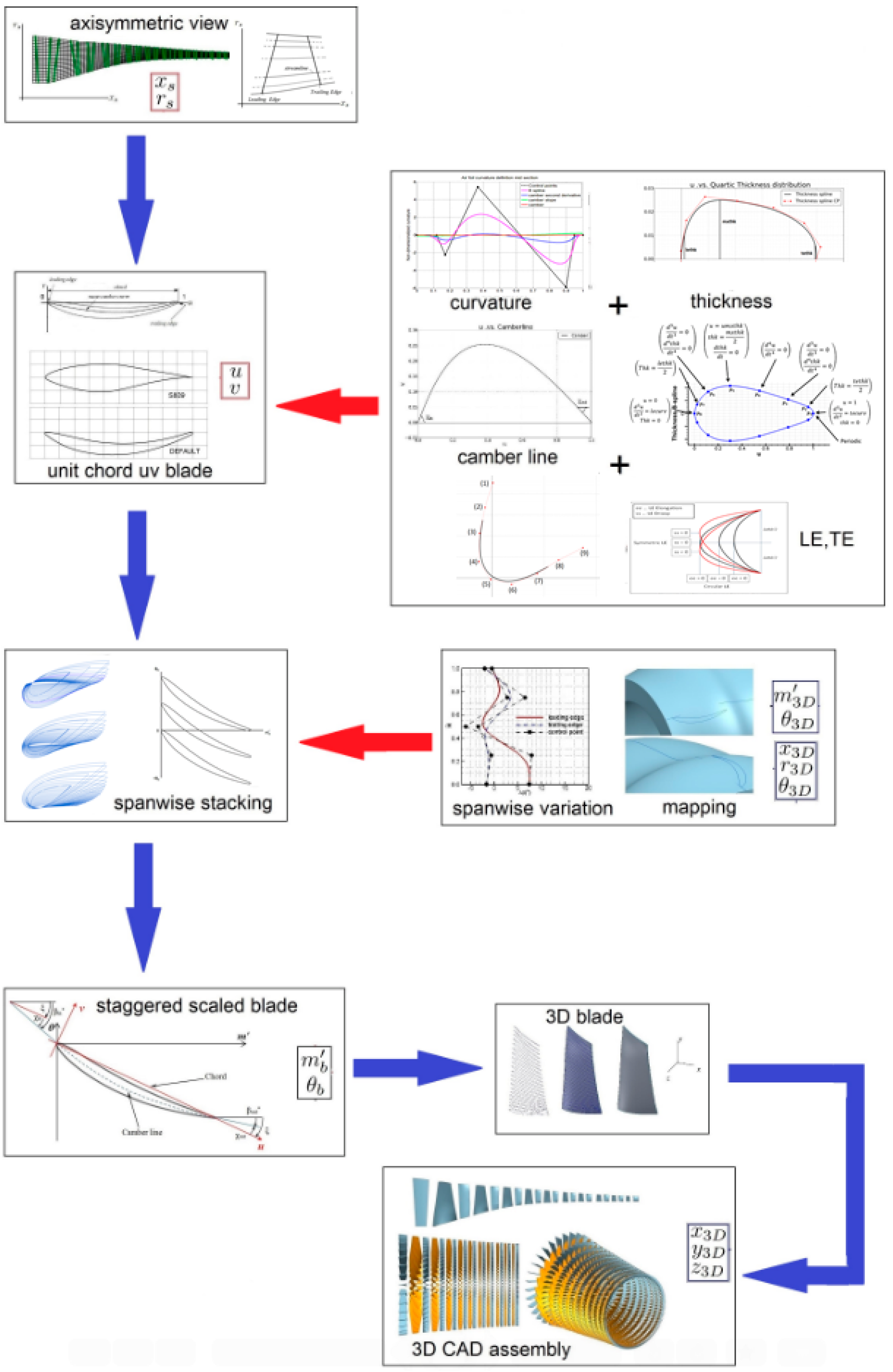
2.1. Overview
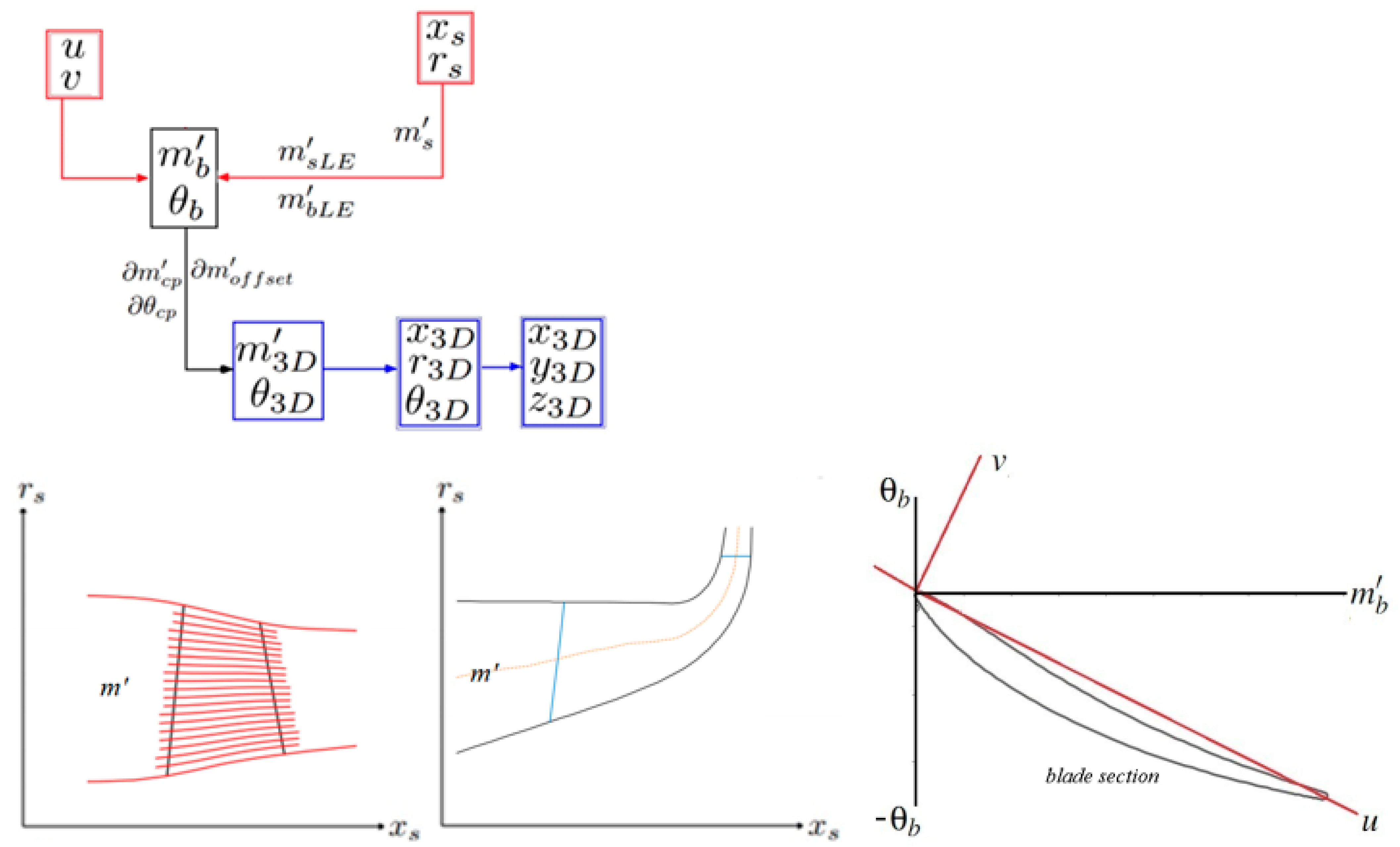
2.2. Coordinate Systems
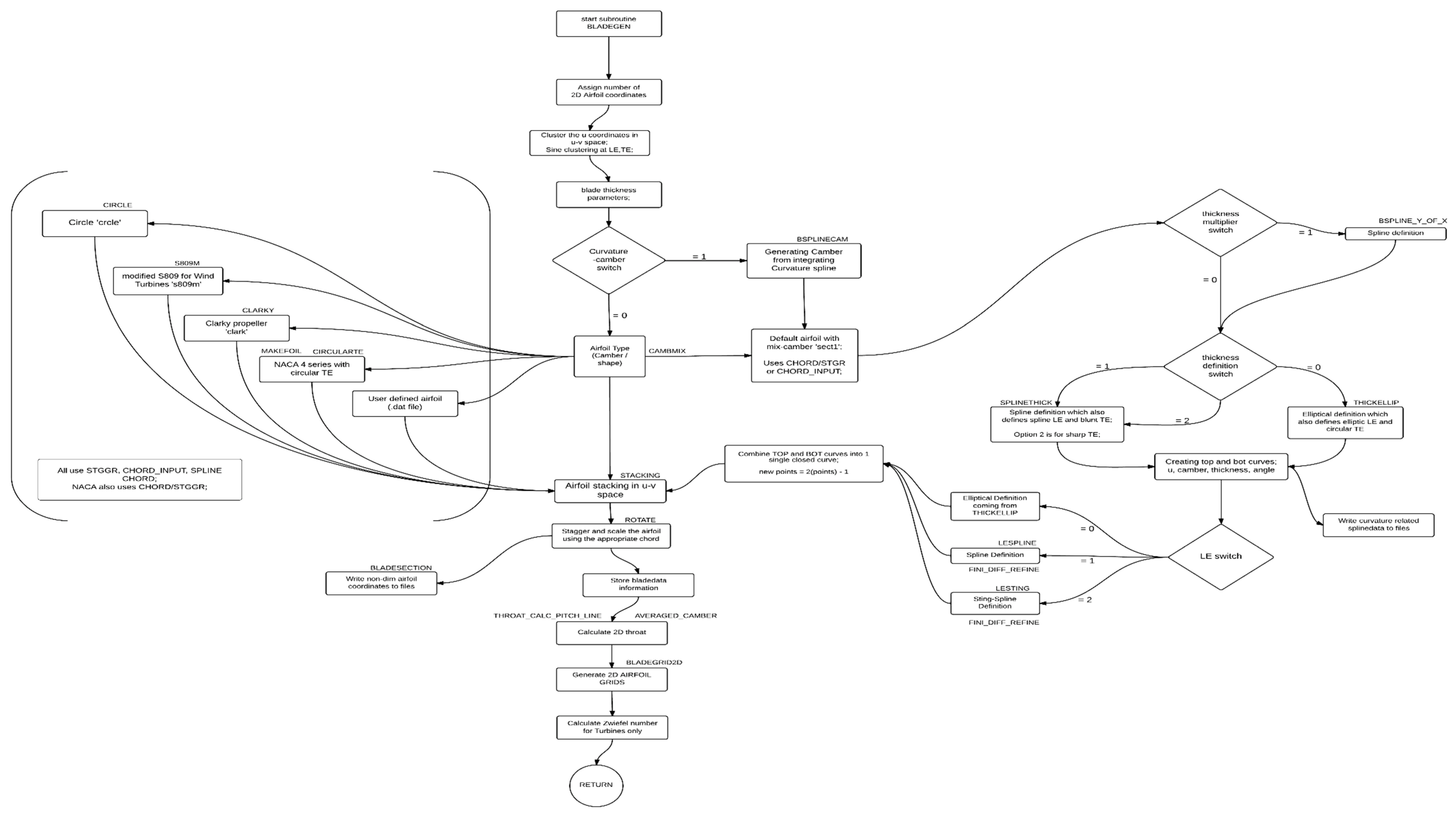
2.3. 2D Airfoil Construction
2.4. Cubic and Quartic B-Spline Implementation for Smoothness
2.5. Streamwise Mapping and Stacking to Obtain 3D Airfoils
2.6. Parameters for Geometry Generation in 2D and 3D
2.7. Blade Visualizers
2.8. Periodic Boundary for Fluid Domain and 2D Grids
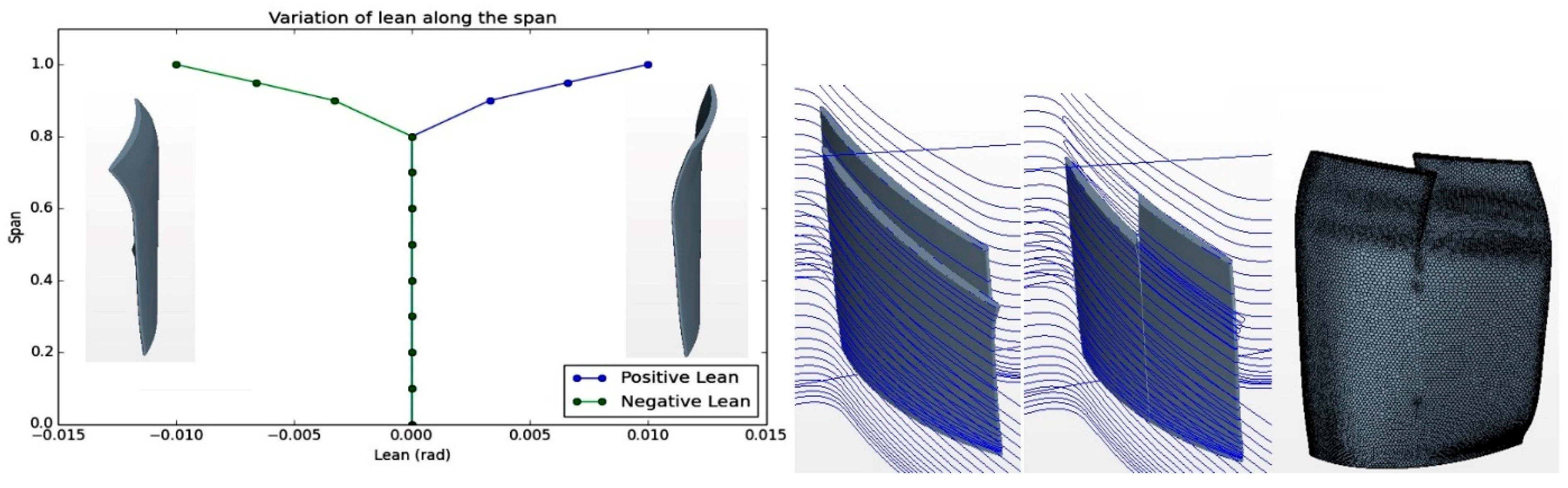
2.9. Splitter Blade, Sweep, and Lean Effect
2.10. Automation, Optimization, and CAD Connection
2.11. 3D Section Offset and Tool Generality
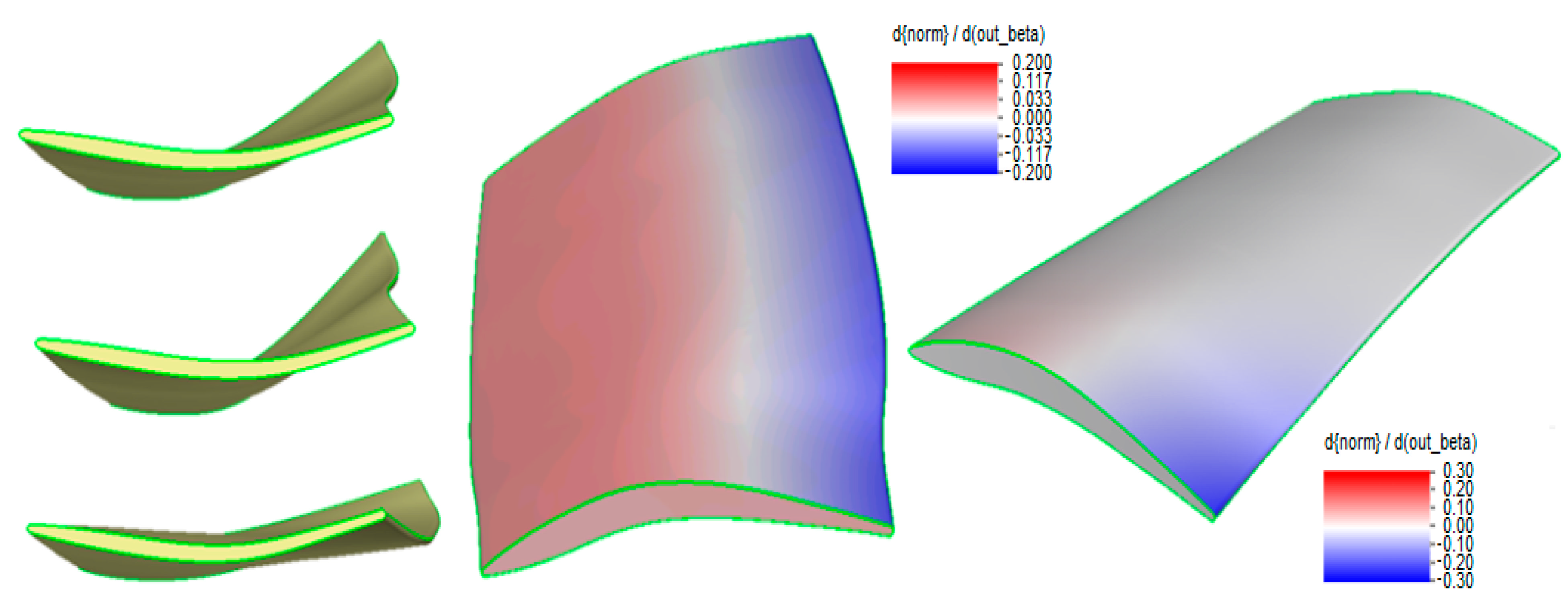
2.12. Parametric Sensitivities
2.13. 3D CFD Simulation Setup and Grid Dependency Study
3. Results
3.1. Ducted Axial Turbomachines
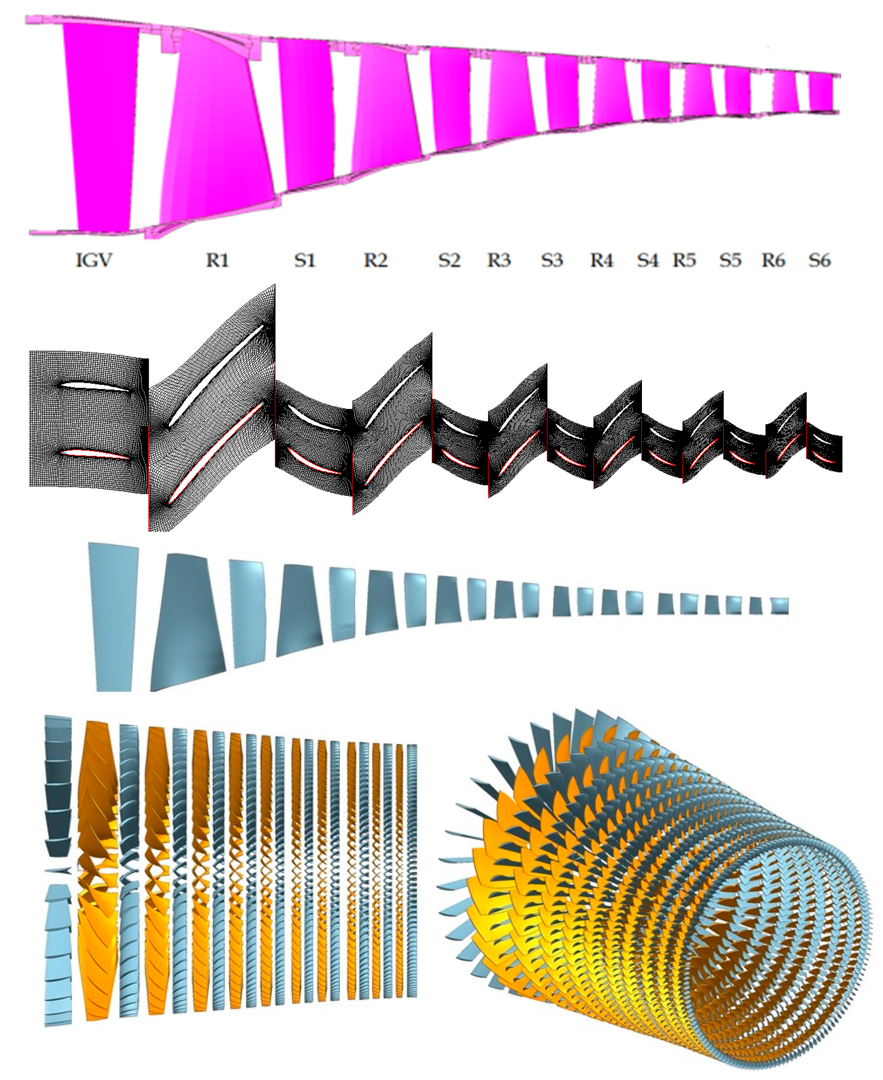
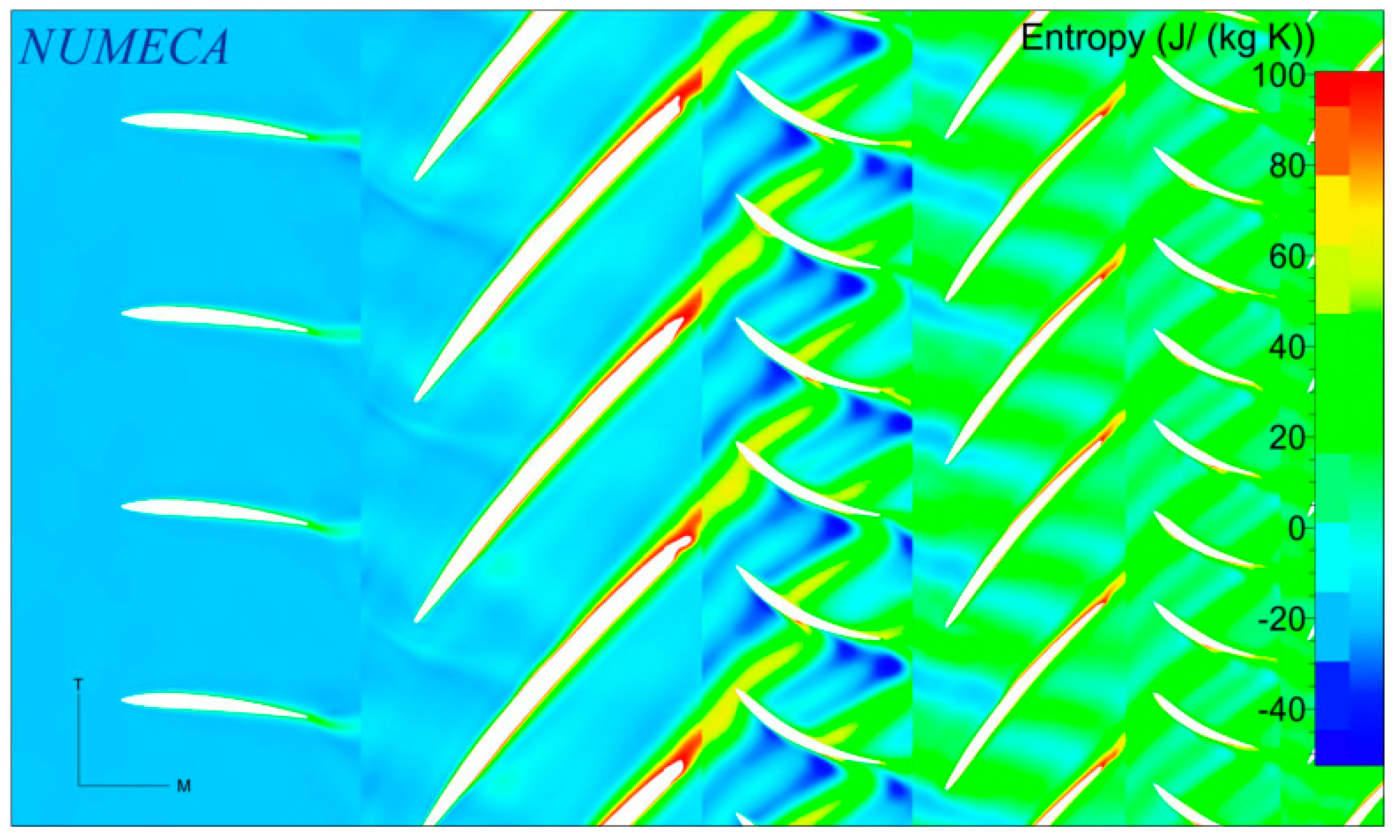
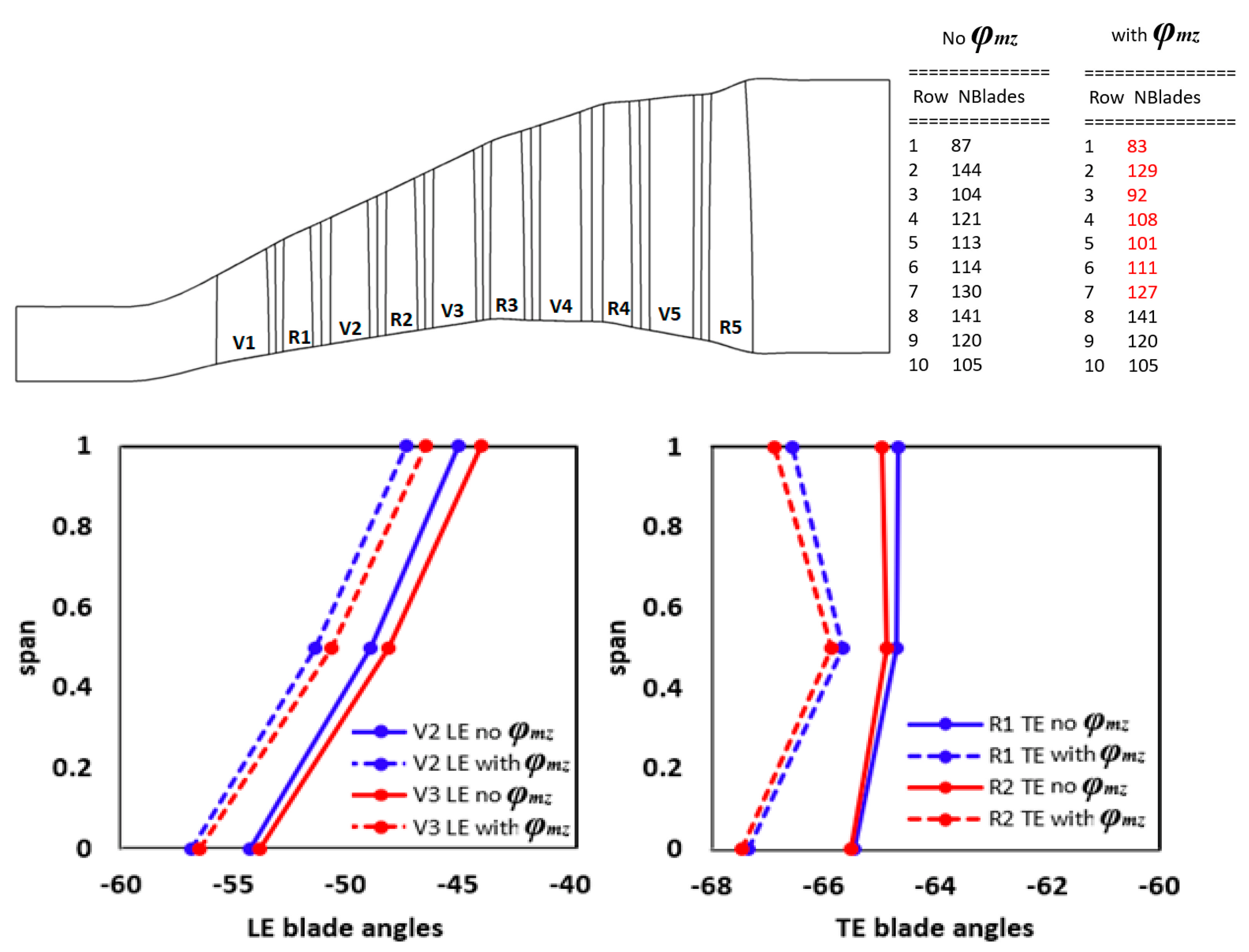
3.1.1. First 6 Stages of 10 Stage E3 HPC
3.1.2. E3 5 Stage LPT
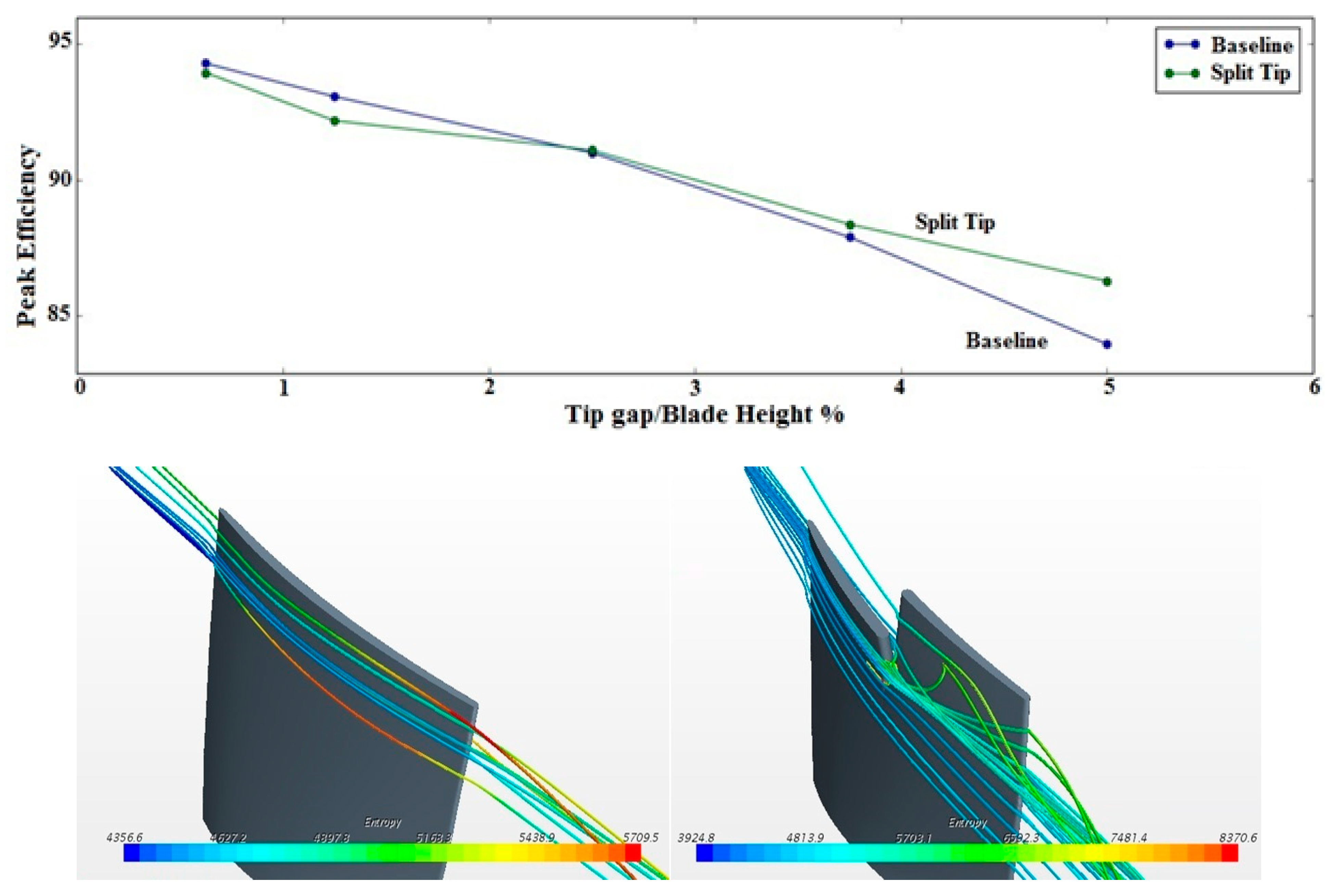
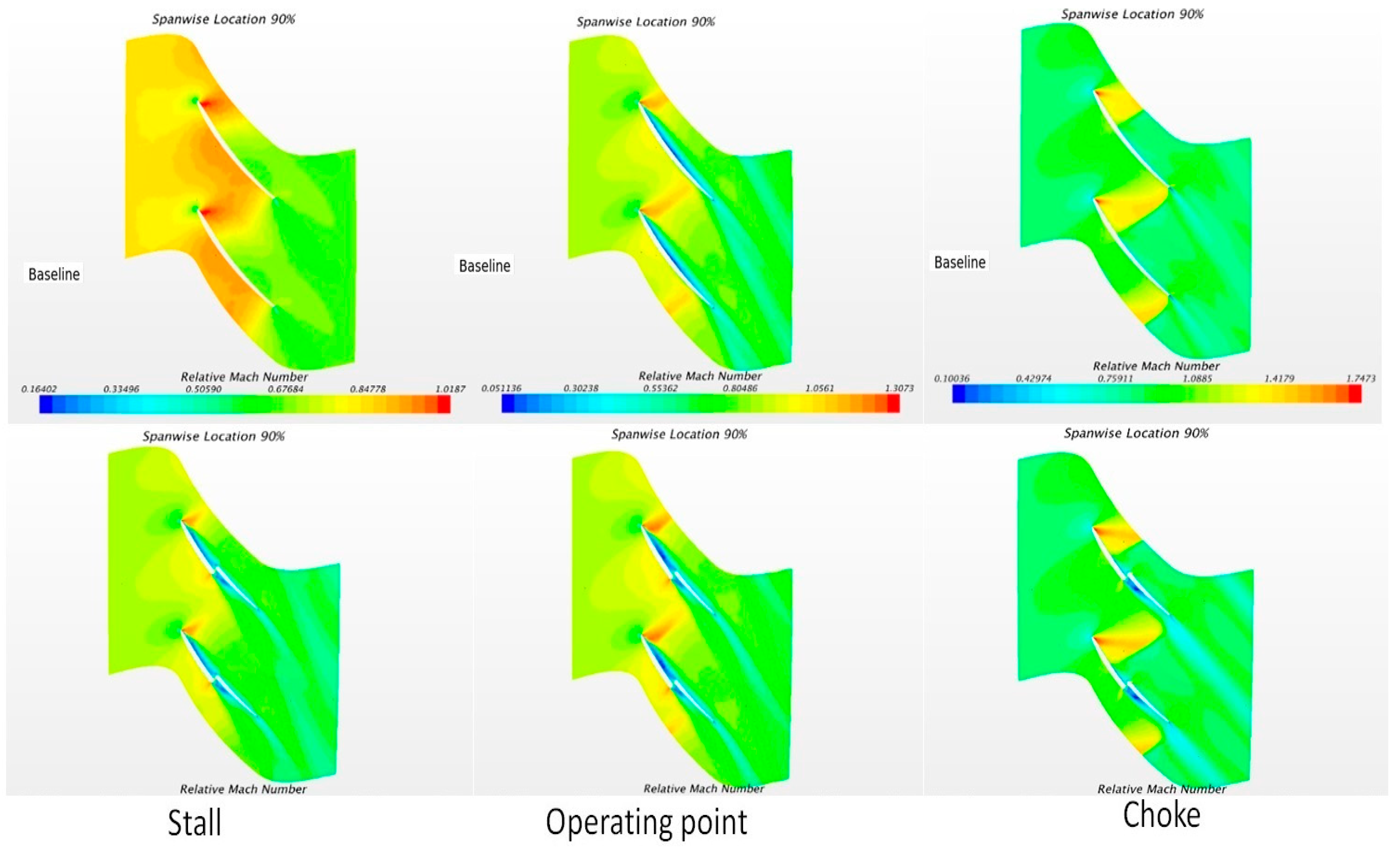
3.1.3. Split Tip E3 HPC Rotor 6
3.1.4. Non-Axisymmetric OGV for Boundary Layer Ingestion Fan
3.2. Ducted Radial Turbomachines
3.2.1. Centrifugal Compressors
3.2.2. Turbopump, Curved LE Impeller, Radial De-Swirler, and Diffuser Vane
3.3. Unducted Turbomachines
3.3.1. Propeller
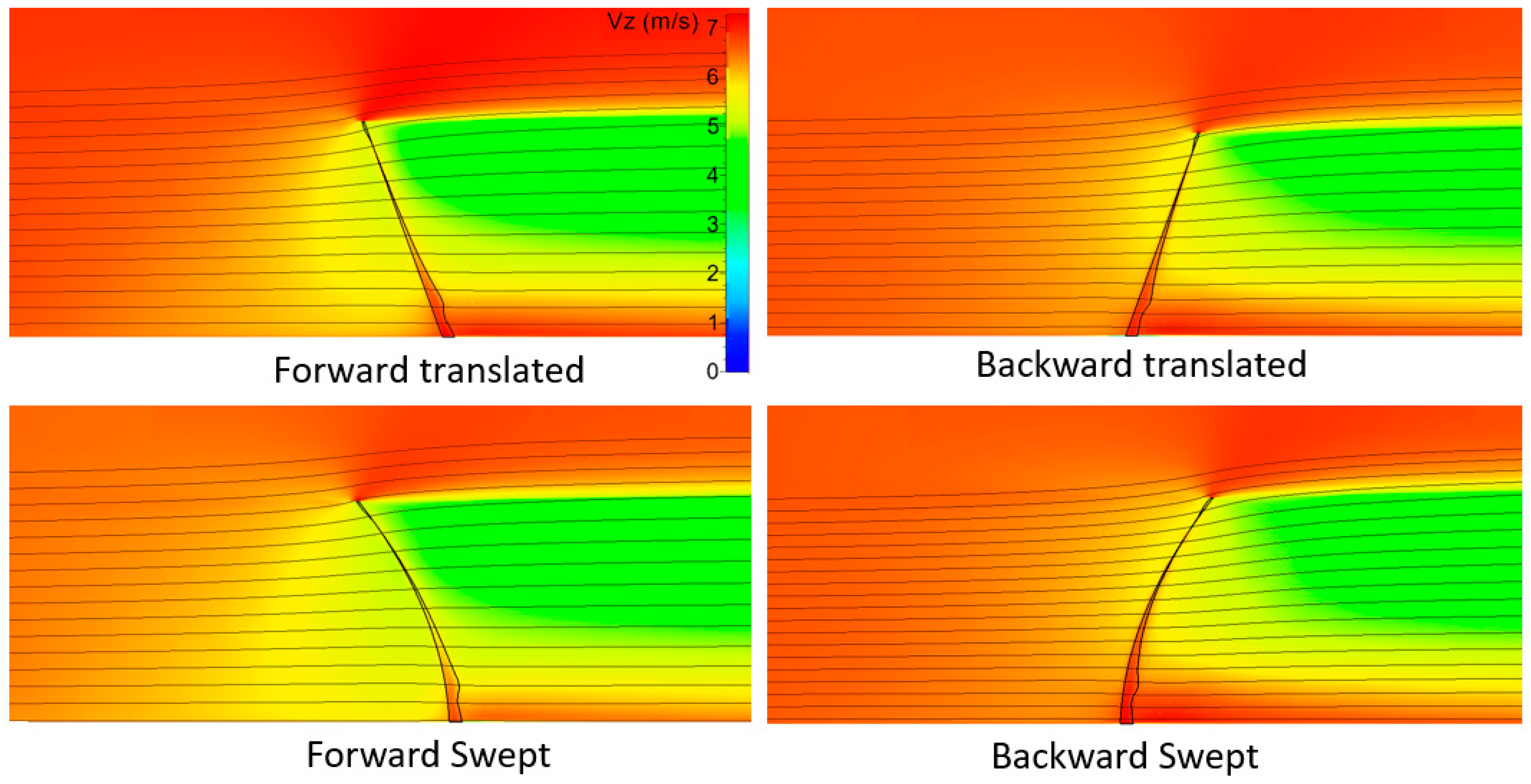
3.3.2. Wind Turbine
3.3.3. Hydrokinetic Turbine
4. Conclusions
Author Contributions
Funding
Institutional Review Board Statement
Informed Consent Statement
Data Availability Statement
Acknowledgments
Conflicts of Interest
Nomenclature
| a | Percent offset |
| b | Intermediate scaling factor |
| B | Basis function |
| CL, CD | Coefficient of lift and drag |
| C | Curvature, parametric curve continuity |
| G | Geometric continuity |
| L | Reference length |
| m | Meridional |
| P | Control point |
| R | Radius of curvature, rotor |
| r | Radial coordinate |
| S | B-spline segment |
| s | Entropy |
| scf | Dimensional blade scaling factor |
| t | Parameter t (0, 1) for spline construction |
| thk | Thickness definition as a function of u |
| u | Normalized chordwise coordinate (0,1) |
| v | Meanline coordinates as a function of u |
| V | Vane |
| x, y, z | Cartesian coordinates |
| y+ | Non-dimensional wall distance |
| α | Angle of attack |
| Ω | Rotational speed of the rotor |
| β, β* | Flow angle, metal angle |
| φ | Slope of streamline |
| ζ | Stagger angle |
| θ | Tangential coordinate |
| AGS | Abu-Ghannam/Shaw |
| BEMT | Blade element momentum theory |
| CAD | Computer-aided design |
| CFD | Computational fluid dynamics |
| E3 | Energy efficient engine |
| HPC | High-pressure compressor |
| KE | Kinetic energy |
| LE | Leading edge |
| LPC | Low pressure compressor |
| NACA | National Advisory Committee for Aeronautics |
| NASA | National Aeronautics and Space Administration |
| NREL | National Renewable Energy Laboratory |
| OGV | Outlet guide vane |
| RANS | Reynolds averaged Navier–Stokes |
| TE | Trailing edge |
| 2D, 3D | Two- and three-dimensional |
Appendix A

References
- Miller, P.L.; Oliver, J.H.; Miller, D.P.; Tweet, D.L. Bladecad: An interactive geometric design tool for turbomachinery blades. In Proceedings of the 41st Gas Turbine and Aeroengine Congress, ASME, Birmingham, UK, 10–13 June 1996. NASA Technical Memorandum 107262. [Google Scholar]
- Kulfan, B.M. A Universal Parametric Geometry Representation Method—“CST”. AIAA 2007-62. 07. In Proceedings of the 45th AIAA Aerospace Sciences Meeting and Exhibit, Reno, NV, USA, 8–11 January 2007. [Google Scholar]
- Kulfan, B.M.; Bussoletti, J.E. Fundamental Parametric Geometry Representations for Aircraft Component Shapes. AIAA 2006-6948. In Proceedings of the 11th AIAA/ISSMO Multidisciplinary Analysis and Optimization Conference, Portsmouth, VA, USA, 6–8 September 2006. [Google Scholar]
- Kulfan, B.M. Universal Parametric Geometry Representation Method. J. Aircr. 2008, 45, 142–158. [Google Scholar] [CrossRef]
- Sripawadkul, V.; Padulo, M.; Guenov, M. A comparison of airfoil shape parameterization techniques for early design optimization. In Proceedings of the 13th AIAA/ISSMO Multidisciplinary Analysis Optimization Conference, Fort Worth, TX, USA, 13–15 September 2010. [Google Scholar]
- Koini, G.N.; Sarakinos, S.S.; Nikolos, I.K. A software tool for parametric design of turbomachinery blades. Adv. Eng. Softw. 2009, 40, 41–51. [Google Scholar] [CrossRef]
- Crouse, J.E.; Gorrell, W.T. Computer Program for Aerodynamic and Blading Design of Multistage Axial-Flow Compressors; Tech. Rep. TP 1946; NASA Lewis Research Center: Cleveland, OH, USA, 1981; pp. 1–110. [Google Scholar]
- Engeli, M.; Zollinger, H.J.; Allemann, J.C. A computer program for the design of turbomachinery blades. In Turbo Expo: Power for Land, Sea, and Air; ASME: New York, NY, USA, 1974; pp. 1–10. [Google Scholar] [CrossRef]
- Casey, M.V. A computational geometry for the blades and internal flow channels of centrifugal compressors. Trans. ASME J. Eng. Power. 1983, 105, 288–295. [Google Scholar] [CrossRef]
- Pierret, S.; Demeulenaere, A.; Gouverneur, B.; Braembussche, V.R. Designing turbomachinery blades with the function approximation concept and the Navier-Stokes equations. In Proceedings of the 8th Symposium on Multidisciplinary Analysis and Optimization, Long Beach, CA, USA, 6–8 September 2000; pp. 1–11. [Google Scholar] [CrossRef]
- Oyama, A.; Liou, M.S.; Obayashi, S. Transonic axial-flow blade optimization: Evolutionary algorithms/three-dimensional Navier-Stokes solver. J. Propuls. Power 2004, 20, 612–619. [Google Scholar] [CrossRef]
- Verstraete, T. CADO: A computer aided design and optimization tool for turbomachinery applications. In Proceedings of the 2nd International Conference on Engineering Optimization, Lisbon, Portugal, 6–9 September 2010; pp. 1–10. [Google Scholar]
- Müller, L.; Verstraete, T. CAD Integrated multipoint adjoint-based optimization of a turbocharger radial turbine. Int. J. Turbomach Propuls. Power 2017, 2, 14. [Google Scholar] [CrossRef]
- Leylek, Z.; Neely, A.J. Development of a blade parametric modeling methodology for design and analysis of computer experiments. In Proceedings of the ASME Turbo Expo GT2015-43109, Montreal, Quebec, Canada, 15–19 June 2015. [Google Scholar]
- Korakianitis, T.P. Design of airfoils and cascades of airfoils. AIAA J. 1989, 27, 455–461. [Google Scholar] [CrossRef]
- Korakianitis, T.P.; Pantazopoulos, G.I. Improved turbine-blade design techniques using 4th-order parametric-spline segments. Comput. Aided Des. 1993, 25, 289–299. [Google Scholar] [CrossRef]
- Korakianitis, T.P.; Hamakhan, I.A.; Resaienia, M.A.; Wheeler, A.P.S.; Avital, E.J.; Williams, J.J.R. Design of high-efficiency turbomachinery blades for energy conversion devices with the three-dimensional prescribed surface curvature distribution blade design (circle) method. Appl. Energy 2012, 89, 215–227. [Google Scholar] [CrossRef]
- Burman, J. Geometry Parameterisation and Response Surface-Based Shape Optimization of Aero Engine Compressors. Ph.D. Thesis, Lulea University of Technology, Norrbotten, Sweden, 2003. [Google Scholar]
- Hamakhan, I.A.; Korakianitis, T.P. Aerodynamic performance effects of leading-edge geometry in gas-turbine blades. Appl. Energy 2010, 87, 1591–1601. [Google Scholar] [CrossRef]
- Song, Y.; Gu, C. Effects of Curvature Continuity of Compressor Blade Profiles on Their Performances. In Proceedings of the ASME Turbo Expo 2014, Düsseldorf, Germany, 16–20 June 2014. [Google Scholar]
- Bi, Q.; Chen, H.; Tong, D.; Lu, Y.; Zou, X. Design Method and Performance Effects of Curvature-Smooth Centrifugal Compressor Blades. In Proceedings of the ASME Turbo Expo 2015, Montreal, Canada, 15–19 June 2015. [Google Scholar]
- Meckstroth, C.; Brown, J. Point Cloud to Parameter: An Inverse Geometric Approach to Probabilistic Design. In Proceedings of the ASME Turbo Expo 2019, Phoenix, AZ, USA, 17–21 June 2019. [Google Scholar]
- McKeand, A.M.; Gorguluarslan, R.M.; Choi, S. A Stochastic Approach for Performance Prediction of Aircraft Engine Components Under Manufacturing Uncertainty. In Proceedings of the ASME 2018 International Design Engineering Technical Conferences and Computers and Information in Engineering Conference, Quebec, Canada, 26–29 August 2018. [Google Scholar]
- Benini, E. Three-dimensional multi-objective design optimization of a transonic compressor rotor. J. Propuls. Power 2004, 20, 462–559. [Google Scholar] [CrossRef]
- Lian, Y.; Liou, M.S. Multi-objective optimization of transonic compressor blade using evolutionary algorithm. J. Propuls. Power 2005, 21, 979–987. [Google Scholar] [CrossRef]
- Ellbrant, L.; Eriksson, L.E.; Martenssion, H. Balancing efficiency and stability in the design of transonic compressor stages. In Proceedings of the ASME Turbo Expo GT2013-94838, San Antonia, Texas, USA, 3–7 June 2013. [Google Scholar]
- Zhang, X.; Qiang, X.; Teng, J.; Yu, W. A new curvature-controlled stacking-line method for optimization design of compressor cascade considering surface smoothness. Proc. Inst. Mech. Eng. Part G J. Aerosp. Eng. 2020, 234, 1061–1074. [Google Scholar] [CrossRef]
- Sharma, M.; Turner, M.G. Continuous Modified NACA Four-Digit Thickness Distribution for Turbomachinery Geometries. AIAA J. 2021, 59, 1501–1505. [Google Scholar] [CrossRef]
- Dannenhoffer, J.F.; Haimes, R. Generation of Multi-fidelity, Multi-discipline Air Vehicle Models with the Engineering Sketch Pad. In Proceedings of the 54th AIAA Aerospace Sciences Meeting, AIAA, 6.2016-1925, San Diego, CA, USA, 4–8 January 2016. [Google Scholar]
- Dannenhoffer, J.F.; Haimes, R. Using Design-Parameter Sensitivities in Adjoint-Based Design Environments. In Proceedings of the 55th AIAA Aerospace Sciences Meeting, AIAA 2017-0139, Grapevine, TX, USA, 9–13 January 2017. [Google Scholar]
- Canfield, R.A.; Alnaqbi, S.; Durscher, R.J.; Bryson, D.E.; Kolonay, R.M. Shape Continuum Sensitivity Analysis using ASTROS and CAPS. In Proceedings of the AIAA Scitech Forum, AIAA, 6.2019-2228, San Diego, CA, USA, 7–11 January 2019. [Google Scholar]
- Meckstroth, C.M. Parameterized, Multi-fidelity Aircraft Geometry and Analysis for MDAO Studies using CAPS. In Proceedings of the AIAA Scitech 2019 Forum, AIAA, 6.2019-2230, San Diego, CA, USA, 7–11 January 2019. [Google Scholar]
- Agromayor, R.; Anand, N.; Müller, J.-D.; Pini, M.; Nord, L. A Unified Geometry Parametrization Method for Turbomachinery Blades. Comput. Aided Des. 2021, 133, 102987. [Google Scholar] [CrossRef]
- Luo, S.; Cui, J.; Sella, V.; Liu, J.; Koric, S.; Kindratenko, V. Turbomachinery Blade Surrogate Modeling using Deep Learning. In ISC High Performance; Springer: Cham, Switzerland, 2021; Lecture Notes in Computer Science 12761. [Google Scholar]
- Shi, H. A Parametric Blade Design Method for High-Speed Axial Compressor. Aerospace 2021, 8, 271. [Google Scholar] [CrossRef]
- Shi, H. Parametric Research and Aerodynamic Characteristic of a Two-Stage Transonic Compressor for a Turbine Based Combined Cycle Engine. Aerospace 2022, 9, 346. [Google Scholar] [CrossRef]
- Yang, J.; Hu, B.; Tao, Y.; Li, J. A flexible method for geometric design of axial compressor blades. Proc. Inst. Mech. Eng. Part G J. Aerosp. Eng. 2022, 236, 2420–2432. [Google Scholar] [CrossRef]
- Sairam, K. The Influence of Radial Area Variation on Wind Turbines to the Axial Induction Factor. Master’s Thesis, University of Cincinnati, Cincinnati, OH, USA, 2013. [Google Scholar]
- Brossman, J.R. An Investigation of Rotor Tip Leakage Flows in the Rear-Block of a Multistage Compressor. Ph.D. Thesis, Purdue University, Pennsylvania, PA, USA, 2012. [Google Scholar]
- Srinivas, A. Novel Compressor Blade Design Study. Master’s Thesis, University of Cincinnati, Cincinnati, OH, USA, 2015. [Google Scholar]
- Syed, M.H.M. Optimization Capabilities for Axial Compressor Blades and Seal Teeth Cavity. Master’s Thesis, University of Cincinnati, Cincinnati, OH, USA, 2016. [Google Scholar]
- Masters, I.; Williams, A.; Croft, T.; Togneri, M.; Edmunds, M.; Zangiabadi, E.; Fairley, I.; Karunarathna, H. A Comparison of Numerical Modelling Techniques for Tidal Stream Turbine Analysis. Energies 2015, 8, 7833–7853. [Google Scholar] [CrossRef] [Green Version]
- Wu, Y.T.; Porte-Agel, F. Atmospheric Turbulence Effects on Wind-Turbine Wakes: An LES Study. Energies 2012, 5, 5340–5362. [Google Scholar] [CrossRef]
- Bhide, K.; Siddappaji, K.; Abdallah, S.; Roberts, K. Improved Supersonic Turbulent Flow Characteristics Using Non-Linear Eddy Viscosity Relation in RANS and HPC-Enabled LES. Aerospace 2021, 8, 352. [Google Scholar] [CrossRef]
- Bhide, K.; Abdallah, S. Turbulence statistics of supersonic rectangular jets using Reynolds Stress Model in RANS and WALE LES. In Proceedings of the AIAA AVIATION 2022 Forum, AIAA 2022-3344, Chicago, IL, USA, 27 June–1 July 2022. [Google Scholar]
- Bhide, K.; Abdallah, S. Anisotropic Turbulent Kinetic Energy budgets in compressible rectangular jets. Aerospace 2022, 9, 484. [Google Scholar] [CrossRef]
- Turner, M.G.; Bruna, D.; Merchant, A. Applications of a turbomachinery design tool for compressors and turbines. In Proceedings of the 43rd AIAA/ASME/SAE/ASEE Joint Propulsion Conference & Exhibit, Cincinnati, OH, USA, 8–11 July 2007; pp. 2007–5152. [Google Scholar]
- Siddappaji, K. On the Entropy Rise in General Unducted Rotors Using Momentum, Vorticity and Energy Transport. Ph.D. Thesis, University of Cincinnati, Cincinnati, OH, USA, 2018. [Google Scholar]
- Denton, J.D. The effects of lean and sweep on transonic fan performance: A computational study. In Turbo Expo: Power of Land Sea and Air; ASME: New York, NY, USA, 2002. [Google Scholar]
- Smith, J.; Leroy, H.; Yeh, H. Sweep and dihedral effects in axial-flow turbomachinery. J. ASME 1963, 85, 401–414. [Google Scholar] [CrossRef]
- Siddappaji, K. Parametric 3d Blade Geometry Modeling Tool for Turbomachinery Systems. Master’s Thesis, University of Cincinnati, Cincinnati, OH, USA, 2012. [Google Scholar]
- Wennerstrom, A.J. Design of Highly Loaded Axial-fow Fans and Compressors; Concepts ETI, Inc.: Windsor, VT, USA, 2000. [Google Scholar]
- Nemnem, A.F.; Turner, M.G.; Siddappaji, K.; Galbraith, M.C. A smooth curvature-defined meanline section option for a general turbomachinery geometry generator. In Proceedings of the ASME Turbo Expo 2014, Dusseldorf, Germany, 16–20 June 2014. [Google Scholar]
- Sharma, M.; Dannenhoffer, J.; Holder, J.; Turner, M.G. Integration of an Open Source Blade Geometry Generator Using a Physics Based Parameterization with the Engineering Sketch Pad. In Proceedings of the ASME Turbo Expo 2020, Virtual, 21–25 September 2020. [Google Scholar] [CrossRef]
- Turner, M.G.; Park, K.; Siddappaji, K.; Dey, S.; Gutzwiller, D.P.; Merchant, A.; Bruna, D. Framework for Multidisciplinary Optimization of Turbomachinery. In Proceedings of the ASME Turbo Expo 2010, Glasgow, UK, 14–18 June 2010; pp. 623–631. [Google Scholar]
- Goodhand, M.N.; Miller, R.J. The impact of real geometries on three-dimensional separations in compressors. In Proceedings of the ASME Paper Number GT2010-22246, Glasgow, UK, 14-18 June 2010. [Google Scholar]
- Vince, J. Mathematics for Computer Graphics, 2nd ed.; Springer: London, UK, 2006. [Google Scholar]
- Hoffmann, I.J.M. On the quartic curve of han. J. Comput. Appl. Math. 2009, 223, 124–132. [Google Scholar]
- Fortin, D. B-spline toeplitz inverse under corner perturbations. Int. J. Pure Appl. Math. 2012, 77, 107–118. [Google Scholar]
- Sherar, P.A. Variational Based Analysis and Modelling Using B-Splines. Ph.D. Thesis, Cranfield University, Cranfield, UK, 2004. [Google Scholar]
- Papp, I.; Hoffmann, M. C2 and G2 continuous spline curves with shape parameters. J. Geom. Graph. 2007, 11, 1–7. [Google Scholar]
- Spekreijse, S.; Boerstoel, J.W. Multiblock Grid Generation. Part I: Elliptic Grid Generation Methods for Structured Grids; NLR TP 96338; National Aerospace Laboratory NLR: Amsterdam, The Netherlands, 1996. [Google Scholar]
- Bauinger, S.; Gannon, A.J.; Hobson, G.V.; Terrell, A.D. Technology Demonstration of a Splittered Transonic Rotor with a Downstream Variable Geometry Tandem Stator. In Proceedings of the ASME Turbo Expo 2017, Charlotte, NC, USA, 26–30 June 2017. [Google Scholar]
- Galbraith, M.C. A Discontinuous Galerkin Chimera Overset Solver. Ph.D. Theses, University of Cincinnati,, Cincinnati, OH, USA, 2013. [Google Scholar]
- Knapke, R.D. High-Order Unsteady Heat Transfer with the Harmonic Balance Method. Ph.D. Theses, University of Cincinnati, Cincinnati, OH, USA, 2015. [Google Scholar]
- Neshat, M.A.; Akhlaghi, M.; Fathi, A.; Khaledi, H. Investigating the effect of blade sweep and lean in one stage of an industrial gas turbine’s transonic compressor. Propuls. Power Res. 2015, 4, 221–229. [Google Scholar] [CrossRef]
- Eldred, M.S.; Adams, B.M.; Haskell, K.; Bohnhoff, W.J.; Eddy, J.P.; Gay, D.M.; William, E.H.; Hough, P.D.; Kolda, T.G.; Swiler, L.P.; et al. DAKOTA Reference Manual, 4.2 ed.; Sandia National Laboratories: Albuquerque, NM, USA, 2008. [Google Scholar]
- Fineturbo/Autogrid5, Numeca. Available online: http://www.numeca.com/en/products/finetmturbo (accessed on 24 December 2020).
- CD-Adapco. Starccm+ User Guide. Available online: https://www.plm.automation.siemens.com/global/en/products/simcenter/STAR-CCM.html (accessed on 24 December 2020).
- Nemnem, A. A General Multidisciplinary Turbomachinery Design Optimization System Applied to a Transonic Fan. Ph.D. Theses, University of Cincinnati, Cincinnati, OH, USA, 2014. [Google Scholar]
- Clark, T. Pressure Mapping and Efficiency Analysis of an EPPLER 857 Hydrokinetic Turbine. Master’s Thesis, University of Cincinnati, Cincinnati, OH, USA, 2017. [Google Scholar]
- Holloway, P.R.; Knight, G.L.; Koch, C.C.; Shaffer, S.J. Energy Efficient Engine High Pressure Compressor Detail Design Report; Technical Report; NASA-CR-165558; General Electric Company: Boston, MA, USA, 1982. [Google Scholar]
- Claus, R.W.; Beach, T.; Turner, M.G.; Siddappaji, K.; Hendricks, E.S. Geometry and simulation results for a gas turbine representative of the energy efficient engine (EEE). Technical report; NASA: Washington, DC, USA, 2015. [Google Scholar]
- Matthys, R.; Mesward, D.; Turner, M.G.; Siddappaji, K. E3 6 Stage Simulation; Turbomachinery Flow Class Project Internal Report; University of Cincinnati: Cincinnati, OH, USA, 2012. [Google Scholar]
- Cherry, D.G.; Lenahan, D.T. Energy Efficient Engine. Low Pressure Turbine Test Hardware Detailed Design Report. NASA CR 167956; NASA: Washington, DC, USA, 1982. [Google Scholar]
- Srinivas, A.; Siddappaji, K.; Turner, M.G. Novel Compressor Blade Design Study; International Society for Air Breathing Engines: Phoenix, AZ, USA, 2015; ISABE-2015-20263. [Google Scholar]
- Kumar, S.; Turner, M.G.; Siddappaji, K.; Celestina, M. Aerodynamic Design System for Non-Axisymmetric Boundary Layer Ingestion Fans. In Proceedings of the ASME Turbo Expo 2018, Oslo, Norway, 11–15 June 2018. [Google Scholar]
- Mandal, P. Design and Optimization of Boundary Layer Ingesting Propulsor. Master’s Thesis, University of Cincinnati, Cincinnati, OH, USA, 2019. [Google Scholar]
- Kumar, S. Non-AXisymmetric Aerodynamic Design-Optimization System with Application for Distortion Tolerant Hybrid Propulsion. Master’s Thesis, University of Cincinnati, Cincinnati, OH, USA, 2020. [Google Scholar]
- Krain, H. Swirling impeller flow. J. Turbomach. 1988, 110, 122–128. [Google Scholar] [CrossRef]
- Hathaway, M.D. Laser Anemometer Measurements of the Three-Dimensional Rotor Flow Field in the NASA Low Speed Centrifugal Compressor; Technical report, NASA Lewis Research Center, Cleveland, OH, USA, ARL-TR-333; 1995.
- Sato, K.; He, L. Effect of rotor-stator interaction on impeller performance in centrifugal compressors. Int. J. Rotating Mach. 1999, 5, 135–146. [Google Scholar] [CrossRef] [Green Version]
- Mishra, S. Developing Novel Computational Fluid Dynamics Technique for Incompressible Flow and Flow Path Design of Novel Centrifugal Compressor. Master’s Thesis, University of Cincinnati, Cincinnati, OH, USA, 2016. [Google Scholar]
- Shaaban, A. Fluid Flow Controller. U.S. Patent US 6589013B2, 5 February 2001. [Google Scholar]
- Muppana, S. Multi-fidelity Design and Analysis of Single Hub Multi-Rotor High Pressure Centrifugal Compressor. Master’s Thesis, University of Cincinnati, Cincinnati, OH, USA, 2018. [Google Scholar]
- Muppana, S.; Siddappaji, K.; Abdallah, S. High Pressure Novel Single Hub Multi-Rotor Centrifugal Compressor: Performance Prediction and Loss Analysis. In Proceedings of the ASME Turbo Expo, GT2019-91967, Phoenix, AZ, USA, 17–21 June 2019. [Google Scholar]
- Guruprasad, A.H.; Raveesha, A.; Sherikar, A.; Siddappaji, K.; Turner, M.G. Effect of Sweep and Translation on Wind Turbine Blades. Turbomachinery Flow Class Project Internal Report; University of Cincinnati: Cincinnati, OH, USA, 2016. [Google Scholar]
- Drela, M. Xfoil. Available online: http://web.mit.edu/drela/public/web/xfoil/ (accessed on 24 December 2013).


Publisher’s Note: MDPI stays neutral with regard to jurisdictional claims in published maps and institutional affiliations. |
© 2022 by the authors. Licensee MDPI, Basel, Switzerland. This article is an open access article distributed under the terms and conditions of the Creative Commons Attribution (CC BY) license (https://creativecommons.org/licenses/by/4.0/).
Share and Cite
Siddappaji, K.; Turner, M.G. Versatile Tool for Parametric Smooth Turbomachinery Blades. Aerospace 2022, 9, 489. https://doi.org/10.3390/aerospace9090489
Siddappaji K, Turner MG. Versatile Tool for Parametric Smooth Turbomachinery Blades. Aerospace. 2022; 9(9):489. https://doi.org/10.3390/aerospace9090489
Chicago/Turabian StyleSiddappaji, Kiran, and Mark G. Turner. 2022. "Versatile Tool for Parametric Smooth Turbomachinery Blades" Aerospace 9, no. 9: 489. https://doi.org/10.3390/aerospace9090489
APA StyleSiddappaji, K., & Turner, M. G. (2022). Versatile Tool for Parametric Smooth Turbomachinery Blades. Aerospace, 9(9), 489. https://doi.org/10.3390/aerospace9090489