Discrete-Time Model Predictive Controller Using Laguerre Functions for Active Flutter Suppression of a 2D wing with a Flap

Abstract

In this paper, a discrete-time model predictive controller using Laguerre orthonormal function-based (LMPC) for active flutter suppression of a two-dimensional wing with a flap is presented. In this work, a linear mathematical state-space model for the pitch, plunge, and flap degrees of freedom under unsteady aerodynamics is derived and used to determine the linear flutter velocity and frequency of the parameters of a selected experimental wing. To verify the model, the open-loop simulation results are compared to an experimental study using the same wing from the literature. The state-space system is then discretized and LMPC with a Kalman filter is designed and tuned using the MATLAB^® simulation environment at a selected speed in the linear flutter region. The predictive control advantage of dealing with input constraints in a systematic manner is explored through a quantitative analysis of the response of both constrained and unconstrained LMPC controllers. The results indicate that theoretically both cases can give excellent performance. However, the input trajectory generated by the unconstrained LMPC is very aggressive in a way that it is considered impractical when compared to the physical limits of an experimental actuator from the literature. The potential of LMPC to achieve a reasonable performance at a significantly lower computational cost compared to the classical model predictive controller (MPC) is investigated by measuring the time required by the same computer to compute the control trajectory for both controllers. The data suggest that LMPC requires remarkably low computational power, which makes it an excellent choice for fast aeroelastic applications.

1. Introduction

Flutter is a self-excited dynamic aeroelastic instability that causes increasing amplitude oscillation in the aeroelastic structure, which can lead to catastrophic structural failure. Flutter results from the interaction between the inertial, elastic and aerodynamic forces. At a certain airspeed (called the flutter speed), the total aeroelastic system’s damping changes from positive (which dissipates energy) to negative due to the existence of aerodynamic forces [1,2,3,4]. Numerous researchers conducted wind tunnel studies on an aeroelastic structure to experimentally demonstrate the flutter. Alizadeh et al. [5] conducted an experimental investigation of the flutter behavior of a cantilever slab wing constructed from a Plexiglas plate in a closed-loop subsonic wind tunnel. The flutter phenomenon is not limited to wings; it may happen to any elastic structure that is subjected to aerodynamic forces, such as bridges, which are often carefully designed within certain limits to minimize flutter. Construction of long span bridges in mountainous areas is likely to be more difficult. Flutter instability during construction is a major challenge due to flexible structural properties and strong winds with large angles of attack [6].

As flight speeds have increased since World War II, flutter has become more important, along with other aeroelastic phenomena. Passive solutions such as mass balancing and structural modifications have been presented and used for many years, but since most of these solutions involve some weight penalty that negatively affects aircraft performance, they have not been beneficial. In addition, maximizing the performance of modern aircraft requires extremely lightweight structures with lower stiffness, which in turn increases the susceptibility to aeroelastic problems such as flutter. Consequently, researchers have begun to consider the use of control technologies in aeroelasticity. If appropriate control measures are taken to prevent flutter as soon as it begins, the onset of flutter can be delayed to a higher airspeed without significantly modifying the structure and reducing weight. This active approach has been shown to be theoretically and experimentally feasible in several important research papers since the 1970s [2,7,8,9].

Active flutter suppression uses a control surface, as shown in Figure 1, whose deflection is controlled by an appropriate control law. The control law is the relationship between the motion of the main wing surface and the deflection of the control surface. This control law is determined by applying methods from control systems theory [10].

Two approaches to the analysis of dynamic aeroelastic instability of airfoils have been presented in the literature. The first approach uses linearized aeroelastic equations to determine the flutter boundary. The other is a nonlinear approach that provides more information about the nature of this boundary, which can cause catastrophic or benign behavior [11,12]. This study is limited to the linear analysis and control of the flutter of a 2D wing.

The earliest work on flutter suppression presented an approach that examines the physical or mathematical structure of the flutter problem to find the mechanisms responsible for flutter and attempt to suppress them. Among these physical approaches, the “aerodynamic energy” method was the most commonly presented in the literature of the time [13]. Later, with the development of control theory, the classical control system design and analysis techniques using the frequency domain became a feature in many works, such as [14], where the standard root locus technique was used. In addition, classical theory based on the Nyquist stability criterion has been used to formulate a control law for the SISO system in other works, such as [15]. Although the methods of classical theory successfully suppressed flutter, they were not practical for dealing with higher order and multivariable systems [16].

Modern control theory techniques based on modeling and analysis of state spaces have been more efficient in dealing with higher order systems and systems with multiple inputs and outputs. These techniques have appeared in recent work. Pole assignment with state feedback has been applied in many studies, e.g., in [2,12]. The optimal method of linear quadratic controller LQR is another successful controller that appears in works such as [17,18,19,20,21].

Transient aerodynamic models have inherent uncertainties. The development of a successful controller must take this aspect into account. In general, utilizing high gain feedback while constructing a linear system controller can achieve robustness to modeling uncertainties, but this reduces the response to high frequency measurement noise. LQG, a linear feedback strategy that incorporates an optimum estimator into the LQR controller, has been employed in [22,23,24] to strike a balance between robustness and noise suppression.

In recent decades, MPC has attracted much attention as an effective tool for industrial system control. MPC is a real-time optimization strategy that computes an optimal control sequence based on knowledge of the plant dynamics (a model) and feedback information (the current state of the plant), as well as a set of constraints at each time step [25].

Predictive control has been around since the early 1970s. However, because it requires high computational power, it was limited to industrial applications that are considered slow dynamic systems, such as chemical factories. However, with recent massive technological improvements in the capabilities and speed of controllers and power electronics, MPC has received more attention as a useful tool for a wider range of applications [26,27].

MPC is a very powerful tool because it solves an optimization problem to find the optimal input trajectory at each time step (real-time optimization). As a result, it is able to take into account the physical constraints of systems that occur in almost every application, where actuators are usually limited in power or speed and ignoring these limits can lead to a degradation of efficiency. In addition, real-time optimization helps to account for measurement errors that may occur due to unmeasured disturbances [28].

However, compared to modern offline control methods, MPC needs to perform many more calculations that require very powerful and expensive processors. Many research efforts have been undertaken to simplify the computations so that MPC can be implemented more easily and effectively, especially on low-power systems. In reference [29], the author presents a design strategy for MPC based on orthonormal functions. This approach requires less computation than classical MPC and therefore it can be used where fast system dynamics are required, such as in aeroelasticity applications [30].

This study aims to investigate the potential effectiveness of using a discrete-time LMPC for active wing flutter suppression application. The study also looks into LMPC advantage over the classical MPC in terms of computational effort required, in addition to the superiority of MPC and LMPC in terms of their capability to deal with input constraints in a systematic manner. These goals are achieved by designing and tuning a LMPC controller, then analyzing the response to an initial condition, in addition to the response to step input with and without input constraints to compare the results. Furthermore, the computational cost of LMPC is compared to the computational cost of a classical MPC using the same computer hardware, through measuring the time required for each controller to compute the input trajectory. LMPC is expected to provide the benefits of real-time optimization with an acceptable computational cost for one of the most important applications of aeroservoelasticity.

2. Theory and Methods

This section summarizes the theory behind the derivation of the aeroelastic mathematical model and the control method implemented, as well as the indices and metrics used to analyze the results.

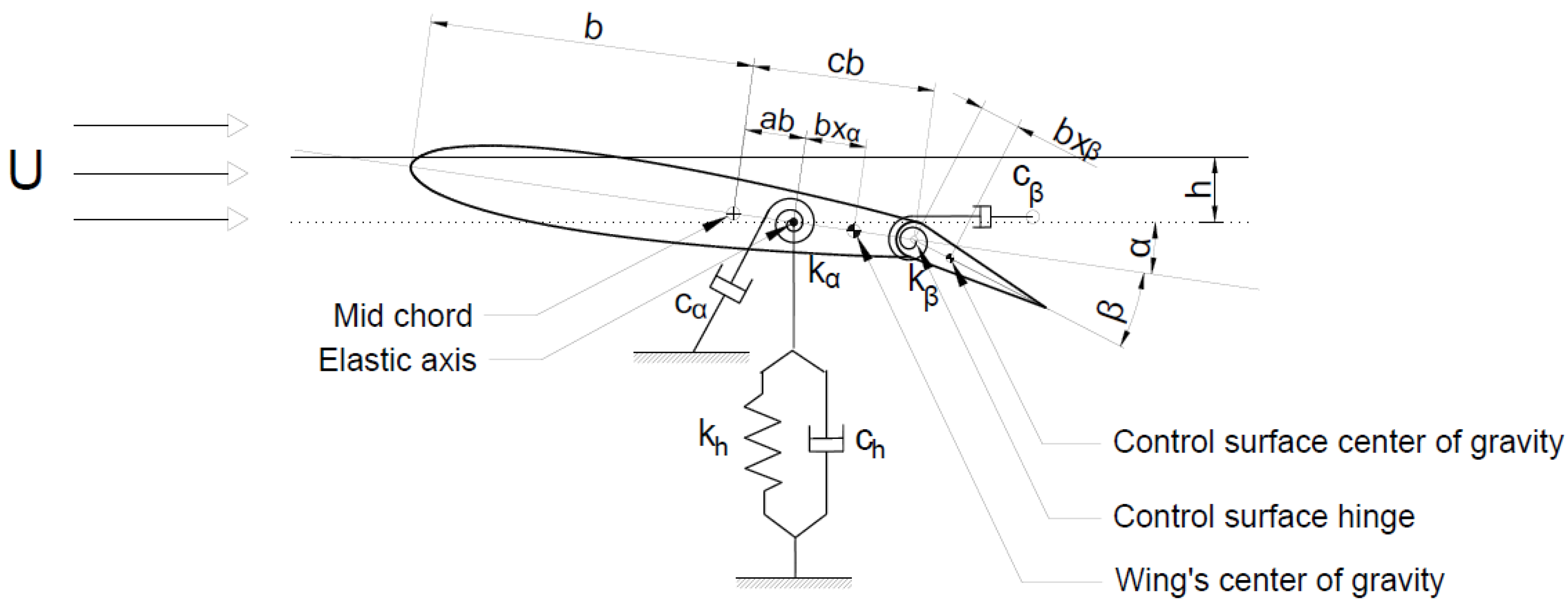
2.1. The Aeroelastic Model

There are several degrees of freedom (DOF) that can occur in a wing during flutter, called ‘flutter modes’, of which two are predominant: the first plunge mode (bending) and the first pitch mode (torsion). As a result of the undesirable coupling of aerodynamic, inertial, and elastic forces, the flutter instability includes two or more vibrational modes and indicates that the structure may successfully absorb energy from the air stream. The damping ratio of the critical flutter mode may decrease with increasing airspeed beyond a certain point. Flutter occurs when the damping ratio of the critical flutter mode reaches zero.

The unsteady aerodynamic forces and moments acting on a 3-DOF wing with pitch, plunge, and flap degrees of freedom have been calculated using a variety of two-dimensional approaches. The Theodorsen approach is applied in this investigation. According to Theodorsen, if a thin airfoil section with infinite aspect ratio and small angle of attack is subjected to minor oscillations in all modes of vibration, the unsteady aerodynamic forces can be estimated as linearly dependent on the exciting structural motion. It is assumed that the flow over the airfoil will stay potential and unseparated [31,32].

Figure 1 describes the physical two-dimensional airfoil with three degrees of freedom (3-DOF) (plunge, pitch, and control flap). The wing is free to plunge (h) (positive downward), pitch ($\alpha$) (positive nose up) about its elastic axis, and the control flap is free to rotate ($\beta$) (positive downward) around its hinge. This model served as the basis for Theodorsen’s development of his unsteady aerodynamics theory [33].

The forces generated due to the airflow are the unsteady aerodynamic lift $L$ (at the elastic axis), the pitching moment $M_{\alpha }$ (about the elastic axis), and the control flap torque $M_{\beta }$ about its hinge. In addition, the flap is equipped with an actuator that can apply a torque $u$ about the hinge line of the control flap relative to the airfoil to control the system [34].

The linearized equations of motion of the system can be represented as:

$$m\ddot{h}+m{x}_{\alpha }b\ddot{\alpha }+m{x}_{\beta }b\ddot{\beta }+c_h\dot{h}+k_h=L$$

(1)

$$I_{\alpha }\ddot{\alpha }+m{x}_{\alpha }b\ddot{h}+\left[\left(c-a\right)b^{2}m{x}_{\beta }+I_{\beta }\right]\ddot{\beta }+c_{\alpha }\dot{\alpha }+k_{\alpha }\alpha =M_{\alpha }$$

(2)

$$m{x}_{\beta }b\ddot{h}+\left[\left(c-a\right)b^{2}m{x}_{\beta }+I_{\beta }\right]\ddot{\alpha }+I_{\beta }\ddot{\beta }+c_{\beta }\dot{\beta }+k_{\beta }\beta =M_{\beta }$$

(3)

where $m$ is the total mass of the wing per unit span, $m_{\beta }$ is the mass of the control surface per unit span. $I_{\alpha }$ is the mass moment of inertia of the wing about its elastic axis per unit span, while $I_{\beta }$ is the mass moment of inertia of the control surface about its hinge line.

The generated aerodynamic forces $L$, $M_{\alpha }\mathrm{and} M_{\beta }$ are represented in terms of the generalized coordinates ($h$, $\alpha$, and $\beta$), in addition to two aerodynamic lag states (${\ell }_1, {\ell }_2$) as follows [24].

$$\begin{array}{cc}\hfill L\left(t\right)& =-\pi {\rho }_{\infty }{b}^2\ddot{h}+\pi {\rho }_{\infty }{b}^{3}a\ddot{\alpha }+{\rho }_{\infty }{b}^3{T}_1\ddot{\beta }-2\pi {\rho }_{\infty }bU\dot{h}-2\pi {\rho }_{\infty }{b}^{2}U\left(1-a\right)\dot{\alpha }\hfill \\ & +{\rho }_{\infty }{b}^{2}U\left(T_4-T_{11}\right)\dot{\beta }-2\pi {\rho }_{\infty }b{U}^2\alpha -2{\rho }_{\infty }b{U}^2{T}_{10}\beta \hfill \\ & +2\pi {\rho }_{\infty }bU{\delta }_{1 }{\ell }_1+2\pi {\rho }_{\infty }bU{\delta }_{2 }{\ell }_2\hfill \end{array}$$

(4)

$$\begin{array}{cc}\hfill M_{\alpha }\left(t\right)& =\pi {\rho }_{\infty }{b}^{3}a\ddot{h}-\pi {\rho }_{\infty }{b}^4\left(\frac{1}{8}+a^2\right)\ddot{\alpha }+{\rho }_{\infty }{b}^4\left(T_7+\left(c-a\right)T_1\right)\ddot{\beta }\hfill \\ & +2\pi {\rho }_{\infty }{b}^{2}U \left(a+\frac{1}{2}\right)\dot{h}-2\pi {\rho }_{\infty }{b}^{3}Ua\left(\frac{1}{2}-a\right)\dot{\alpha }\hfill \\ & +{\rho }_{\infty }{b}^{3}U\left(T_8-T_1+\left(c-a\right)T_4+a{T}_{11}\right)\dot{\beta }\hfill \\ & +{\rho }_{\infty }{b}^2{U}^2\left(2a{T}_{10}-T_4\right)\beta + 2\pi {\rho }_{\infty }{b}^2{U}^2 \left(a+\frac{1}{2}\right)\alpha \hfill \\ & -2\pi {\rho }_{\infty }{b}^{2}U \left(a+\frac{1}{2}\right){\delta }_{1 }{\ell }_1 -2\pi {\rho }_{\infty }U{b}^2 \left(a+\frac{1}{2}\right){\delta }_{2 }{\ell }_2\hfill \end{array}$$

(5)

$$\begin{array}{cc}\hfill M_{\beta }\left(t\right)& ={\rho }_{\infty }{b}^3{T}_1\ddot{h}-2{\rho }_{\infty }{b}^4{T}_{13}\ddot{\alpha }+{\rho }_{\infty }{b}^4\frac{1}{\pi }{T}_3\ddot{\beta }-{\rho }_{\infty }{b}^{2}U{T}_{12}\dot{h}\hfill \\ & +{\rho }_{\infty }{b}^{3}U\left[2T_9+T_1+\left(T_4-T_{12}\right)\left(\frac{1}{2}-a\right)\right]\dot{\alpha }\hfill \\ & +{\rho }_{\infty }{b}^{3}U\frac{1}{2\pi }{T}_{11}\left(T_4-T_{12}\right)\dot{\beta }-{\rho }_{\infty }{b}^2{U}^2{T}_{12}\alpha -{\rho }_{\infty }{b}^2{U}^2\frac{1}{\pi }[T_5\hfill \\ & -T_{10}(T_4-T_{12})]\beta +{\rho }_{\infty }U{b}^2{T}_{12}{\delta }_{1 }{\ell }_1+{\rho }_{\infty }U{b}^2{T}_{12}{\delta }_{2 }{\ell }_2\hfill \end{array}$$

(6)

where ${\rho }_{\infty }$ is the air density, $U$ is the airspeed, and the geometric coefficients $T_i ,i=1,2,\dots$ are called Theodorsen constants, which are functions of the non-dimensional distances $c$ and $b$ defined in the wing model, making them specific to a typical sectional model. Theodorsen constants are given in the report of Theodorsen [35]. These constants are given in Appendix A.

The complete system equations combining Equations (1)–(3) with (4)–(6) are presented in matrix form as

$$\left[{ \overline{\mathrm{M}}}_{\mathrm{s}}-{ \overline{\mathrm{M}}}_{\mathrm{a}}\right] \left\{\begin{array}{c}\ddot{h}/b\\ \ddot{\alpha }\\ \ddot{\beta }\end{array}\right\}+\left[{ \overline{\mathrm{D}}}_{\mathrm{s}}-{ \overline{\mathrm{D}}}_{\mathrm{a}}\right] \left\{\begin{array}{c}\dot{h}/b\\ \dot{\alpha }\\ \dot{\beta }\end{array}\right\}+\left[{ \overline{\mathrm{K}}}_{\mathrm{s}}-{ \overline{\mathrm{K}}}_{\mathrm{a}}\right] \left\{\begin{array}{c}h/b\\ \alpha \\ \beta \end{array}\right\}={ \overline{\mathrm{L}}}_{\mathsf{\delta }}\left\{\begin{array}{c}{\ell }_1\\ {\ell }_2\end{array}\right\}+{ \overline{\mathrm{L}}}_{\mathrm{c}}\left\{{\beta }_c\right\}$$

(7)

Equation (7) can be presented in the following standard state-space representation

$$\begin{gathered} \dot{x}=\mathrm{A}x+\mathrm{B}u \\ y=\mathrm{C}x+\mathrm{D}u \end{gathered}$$

(8)

The details of the matrices of Equations (7) and (8) are given in Appendix B. In the next section, the state space Equations (8) are discretized using MATLAB^®, so that the MPC controller can be added as explained in the next section.

2.2. Discrete Time MPC Using Laguerre Fnctions

A brief explanation of the implemented MPC strategy is given in this section, and more details can be found in Ref. [29]. MPC is usually implemented in discrete time. The general discrete-time state space model of the plant is described by

$$\begin{gathered} x_m\left(k+1\right)=A_m{x}_m\left(k\right)+B_{m}u\left(k\right)+w\left(k\right) \\ y\left(k\right)=C_m{x}_m\left(k\right)+v\left(k\right) \end{gathered}$$

(9)

Here $A_m$ is the discrete system matrix, $B_m$ is the discrete input matrix, and $C_m$ is the discrete output matrix. The system has $n_1$ states, $m$ inputs and $q$ outputs. $u\left(k\right)$ is the vector of manipulated variables (inputs), $x_m\left(k\right)$ is the state vector, and $w\left(k\right)$ is the input disturbance, and $v\left(k\right)$ is the measurement noise. Both are assumed to be sequences of integrated white noise.

To eliminate steady state errors and in the presence of uncertainties or disturbances, it is necessary to embed integrators in the model [36].

By defining a new vector for the state variable $x\left(k\right)={[\begin{array}{cc}\Delta x_m{\left(k\right)}^T& y{\left(k\right)}^T\end{array}]}^T$, it is shown that the original plant model is augmented by an integrator and represented as follows

$$\begin{gathered} \left[\begin{array}{c}\Delta x_m\left(k+1\right)\\ y\left(k+1\right)\end{array}\right]=\left[\begin{array}{cc}{A}_m& o_m^T\\ C_m{A}_m& I_{q\times q}\end{array}\right]\left[\begin{array}{c}\Delta x_m\left(k\right)\\ y\left(k\right)\end{array}\right]+\left[\begin{array}{c}{B}_m\\ C_m{B}_m\end{array}\right]\Delta u\left(k\right)+\left[\begin{array}{c}{B}_d\\ C_m{B}_d\end{array}\right]ϵ\left(k\right) \\ y\left(k\right)=\left[\begin{array}{cc}{o}_m& I_{q\times q}\end{array}\right]\left[\begin{array}{c}\Delta x_m\left(k\right)\\ y\left(k\right)\end{array}\right] \end{gathered}$$

(10)

where $I_{q\times q}$ is an identity matrix with $q\times q$ elements, and $o_m$ is a $q\times n_1$ zero matrix and

$$w\left(k\right)-w\left(k-1\right)=ϵ\left(k\right)$$

(11)

For simplicity, the discrete state space system with an embedded integrator (augmented model) is represented as follows

$$\begin{gathered} x\left(k+1\right)=Ax\left(k\right)+B\Delta u\left(k\right)+B_{ϵ}ϵ\left(k\right) \\ y\left(k\right)=Cx\left(k\right) \end{gathered}$$

(12)

where

$$\begin{gathered} A=\left[\begin{array}{cc}{A}_m& o_m^T\\ C_m{A}_m& I_{q\times q}\end{array}\right];B=\left[\begin{array}{c}{B}_m\\ C_m{B}_m\end{array}\right]; \\ {B}_{ϵ}=\left[\begin{array}{c}{B}_d\\ C_m{B}_d\end{array}\right];C=\left[\begin{array}{cc}{o}_m& I_{q\times q}\end{array}\right] \end{gathered}$$

(13)

The dimensionality of the augmented state-space equation is $n$ which is equal to $n_1+q$.

Define $k_i$ as the sampling time. Then, the current plant states are denoted by $x(k_i)$, and the future control trajectory is:

$$\Delta U=\left[\Delta u{\left(k_i\right)}^T \Delta u{\left(k_i+1\right)}^T \dots \Delta u{\left(k_i+N_c-1\right)}^T\right]{ }^T$$

(14)

where $N_c$ is called the control horizon, which is the number of parameters used for the future control trajectory.

The future state variables are:

$$x\left(k_i+1 | k_i\right) x\left(k_i+2 | k_i\right) \dots x\left(k_i+m | k_i\right) x\left(k_i+N_p | k_i\right)$$

(15)

where $x\left(k_i+m | k_i\right)$ is the predicted state variable at instant $m$ given the current plant information. $N_p$ is called the prediction horizon and represents the optimization window such that $N_c\le N_p$.

To reduce the computational effort, an MPC method based on orthonormal Laguerre functions was chosen for this study. This method is proposed for applications where rapid system dynamics is required [30,37].

In this method, the control trajectory $\Delta U$ is expressed by a set of orthonormal functions called Laguerre functions. The Laguerre networks are known for their orthonormality. The z-transforms of the discrete-time Laguerre networks are written as

$$\begin{gathered} {\mathsf{\Gamma }}_1\left(z\right)=\frac{\sqrt{1-a^2}}{1-a{z}^{-1}} \\ {\mathsf{\Gamma }}_2\left(z\right)=\frac{\sqrt{1-a^2}}{1-a{z}^{-1}}\frac{z^{-1}-a}{1-a{z}^{-1}} \\ ⋮ \\ {\mathsf{\Gamma }}_N\left(z\right)=\frac{\sqrt{1-a^2}}{1-a{z}^{-1}}{\left(\frac{z^{-1}-a}{1-a{z}^{-1}}\right)}^{N-1} \end{gathered}$$

(16)

where $a$ is the pole of the discrete-time Laguerre network. $a$ is also called the scaling factor and must be selected by the user. To ensure the stability of the network, $a$ should be $0 \le a\le 1$.

$N$ is the order of the Laguerre network and is used to capture the control signal. $N$ has a similar function to the control horizon in classical MPC.

The inverse z-transform of ${\mathsf{\Gamma }}_N\left(z\right)$ is denoted by $l_N\left(k\right)$, thus the set of discrete-time Laguerre functions for $i=1, \dots , m$ inputs is represented in vector form as

$$L_i\left(k\right)=\left[l_1\left(k\right) l_2\left(k\right) \dots l_N\left(k\right)\right]{ }^T$$

(17)

$L_i\left(k\right)$ is solved as follows

$$L_i\left(k+1\right)=A_l{}_i{L}_i\left(k\right)$$

(18)

where $A_l{}_i$ is a $\left(N\times N\right)$ matrix and a function of $a$ and $\beta =\left(1-a^2\right)$.

The initial condition of Equation (18) is

$$L_i\left(0\right)=\sqrt{\beta }{\left[1 -a a^2 \dots {\left(-1\right)}^{N-1}{a}^{N-1}\right]}^T$$

(19)

At time instant $k_i$, the control trajectory (14) is considered as the impulse response of a stable dynamical system. Therefore, a set of Laguerre functions, $l_1\left(k\right), l_2\left(k\right), \dots , l_N\left(k\right)$ is used to capture this response with a set of Laguerre coefficients $c_j$ determined during the design. At any arbitrary future time instant $k$, the control input $\Delta u\left(k_i+k\right)$ is represented as

$$\Delta u\left(k_i+k\right)={\displaystyle \sum }_{j=1}^N{c}_j\left(k_i\right)l_j\left(k\right)=L_i{\left(k\right)}^T{\eta }_i$$

(20)

where η_i = [c₁ c₂ … c_N]^T, and $c_j$ are functions of the initial time instant of the moving horizon window $k_i$.

The control horizon $N_c$ from classical MPC disappears here. Instead, the number of terms $N$ and the parameter $a$ are used to describe the complexity of the control trajectory.

The goal now is to find the optimal coefficient vector $\eta$ that minimizes the cost function $J$, which is represented as

$$J={\displaystyle \sum }_{m=1}^{N_p}x{(k_i+m |k_i)}^{T}Q x(k_i+m |k_i)+{\eta }^T R \eta$$

(21)

where $Q$ and $R$ are symmetric, positive definite weight matrices chosen by the designer.

Once the optimal coefficient vector $\eta$ is found, the receding horizon control law is obtained using Equation (20), which is written in terms of linear state feedback control as follows [29].

$$\Delta u\left(k\right)=-K_{mpc}x\left(k\right)$$

(22)

where

$$K_{mpc}=L_i{\left(0\right)}^T\left({\left({{\displaystyle \sum }}_{m=1}^{N_p}\varphi \left(m\right)Q \varphi {\left(m\right)}^T+R\right)}^{-1}{{\displaystyle \sum }}_{m=1}^{N_p}\varphi \left(m\right)Q{A}^m\right)$$

(23)

or it can be written as

$$K_{mpc}=L_i{\left(0\right)}^T{\Omega }^{-1}\Psi$$

(24)

where $\varphi {\left(m\right)}^T={\displaystyle \sum }_{i=0}^{m-1}{A}^{m-i-1}BL{\left(i\right)}^T$ is the convolution sum to compute the prediction of the augmented state space system of Equation (10), $\Omega ={\displaystyle \sum }_{m=1}^{N_p}\varphi \left(m\right)Q \varphi {\left(m\right)}^T+R$ and $\Psi ={\displaystyle \sum }_{m=1}^{N_p}\varphi \left(m\right)Q{A}^m$.

Since the prediction of future states is based on the current information about $x(k_i)$, the set point information is contained in $x(k_i)$ as

$$\begin{gathered} x\left(k_i\right)=\left[\begin{array}{c}\Delta x_m\left(k_i\right)\\ e\left(k_i\right)\end{array}\right] \\ e\left(k_i\right)=y\left(k_i\right)-r\left(k_i\right) \end{gathered}$$

(25)

and $K_{mpc}$ gain is rewritten and divided into two parts as

$$K_{mpc}=\left[\begin{array}{cc}{K}_x& K_e\end{array}\right]$$

(26)

Equation (26) is used to represent the closed loop of the discrete-time MPC system using the Laguerre function as

$$\begin{gathered} \left[\begin{array}{c}\Delta x_m\left(k+1\right)\\ y\left(k+1\right)\end{array}\right]=\left(A-B{K}_{mpc}\right)\left[\begin{array}{c}\Delta x_m\left(k\right)\\ y\left(k\right)\end{array}\right]+B{K}_{e}y\left(k\right) \\ y\left(k\right)=C\left[\begin{array}{c}\Delta x_m\left(k\right)\\ y\left(k\right)\end{array}\right] \end{gathered}$$

(27)

Operational constraints are known to be a reason for performance deterioration of the control system when the control signals from the original design meet them. The ability to deal with hard constraints is one of the main features of the MPC. In this study, the constraint on the amplitude of the control signal and its rate of change is considered.

Using the Laguerre functions in the design, the incremental control signal is represented by

$$\Delta u\left(k_i+m\right)=L{\left(m\right)}^T\eta$$

(28)

The constraints are processed as linear inequalities and combined with the cost function. In other words, the optimization procedure now consists of minimizing the cost function $J$ while ensuring that

$$\Delta u^{min}\le \Delta u\left(k_i+m\right)\le \Delta u^{max}$$

(29)

and

$$u^{min}\le u\left(k_i+m\right)\le u^{max}$$

(30)

In principle, all constraints are defined within the prediction horizon. The controller calculates the input trajectory at each time step and implements only the first step of the calculated trajectory if it is within the set limits. However, if, for example, the first step of the input $u$ is greater than the maximum limit $u^{max}$, then the controller would implement the value of $u^{max}$; then, it would reoptimize and calculate a new input trajectory at the next time step. These limits are implemented in the code for calculating the control trajectory after determining the affected matrices [29].

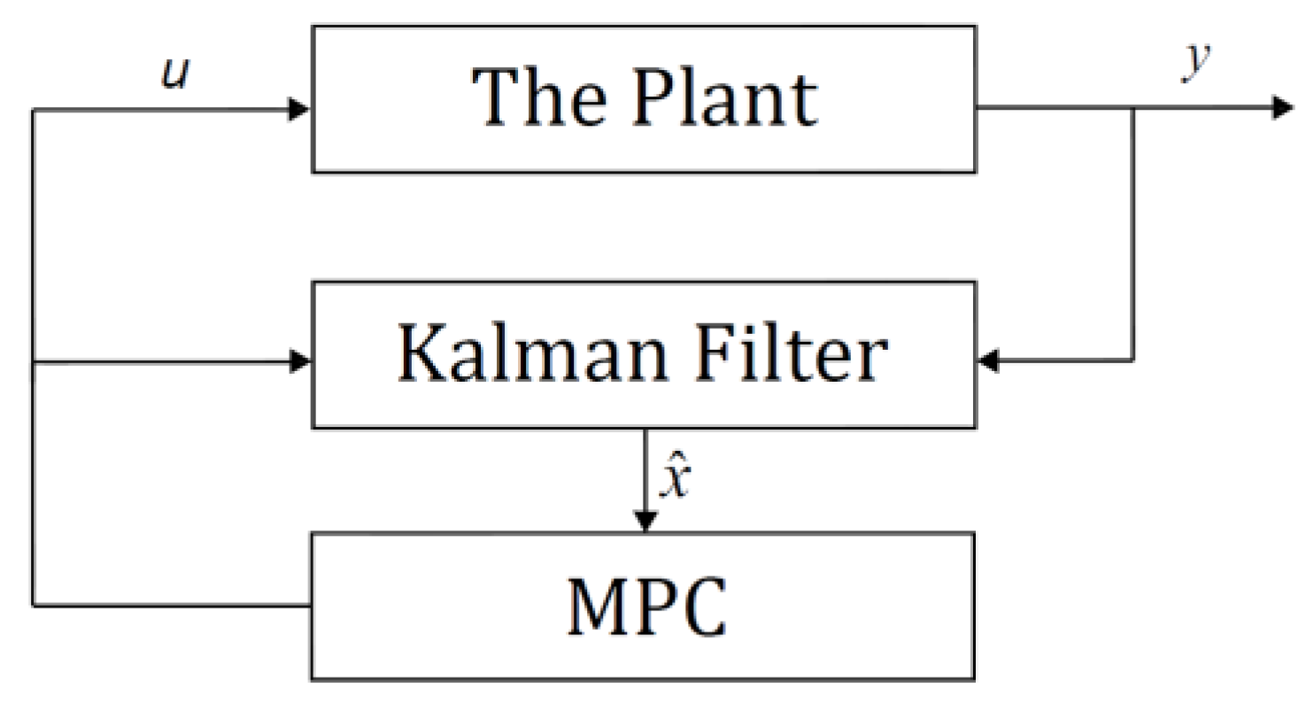
2.3. Discrete Time Kalman Filter

The general discrete-time state-space model of the plant with process noise and measurements $v\left(k\right)$ and $w\left(k\right)$ is described by Equation (9) in Section 2.2. These are assumed to be integrated white noise sequences with covariances $Q_K$ and $R_K$ [38].

The discrete time Kalman filter is a feedback controller that estimates the state variables from the system model and the available measured outputs. Thus, if $A_m$ and $C_m$ are observable quantities, then the control law is computed using the estimated state variables, which are as follows

$$\widehat{x}\left(k_i+1\right)=A\widehat{x}\left(k_i\right)+B\Delta u\left(k_i\right)+K_{obs}\left(y\left(k_i\right)-C\widehat{x}\left(k_i\right)\right)$$

(31)

where $\widehat{x}\left(k_i\right)$ is the current state of the observer, and $K_{obs}$ is the Kalman filter found by solving the discrete time Riccati equation [29,39].

$$P\left(k+1\right)=AP{A}^T-AP{C}^T{\left(R_K+CP{C}^T\right)}^{-1}CP{A}^T+Q_K$$

(32)

then

$$K_{obs}\left(k\right)=AP{C}^T{\left(R_K+CP{C}^T\right)}^{-1}$$

(33)

where, the covariances $Q_K$ and $R_K$ are used as weighting matrices for the filter to tradeoff between the measured values and the values estimated by the model. A block diagram for the closed loop system with Kalman filter is shown in Figure 2.

2.4. Simulation Results Analysis

Controller performance is quantitatively assessed through several performance measures and indices. In this study, three performance metrics are used to compare the step responses of different systems:

• The 10–90% rise time $T_r$ to give an indication of the speed of the response.
• The present overshoot, $P.O.$, which measures the similarity with which the actual response matches the step input.
• The settling time, $T_s$, which indicates how quickly the system settles within 2% of the input amplitude.

In addition to these measures, the integral of the square of the error, ISE, is used as a performance indicator. It is defined as

$$ISE=\underset{0}{\overset{T}{{\displaystyle \int }}}{e}^2\left(t\right) dt$$

(34)

where the error $e$ is the difference between the input and output signals and the upper limit of the integral $T$ is the settling time [40].

Similarly, the integral of the control action (ISU) associated with the input $u$ is [27]

$$ISU=\underset{0}{\overset{T}{{\displaystyle \int }}}{u}^2\left(t\right) dt$$

(35)

3. Results and Discussion

In this section, the open-loop system is analyzed, then the closed-loop system is designed, tuned, and simulated. The results of both systems—which are restricted to a linear system with no control delay—are plotted and discussed.

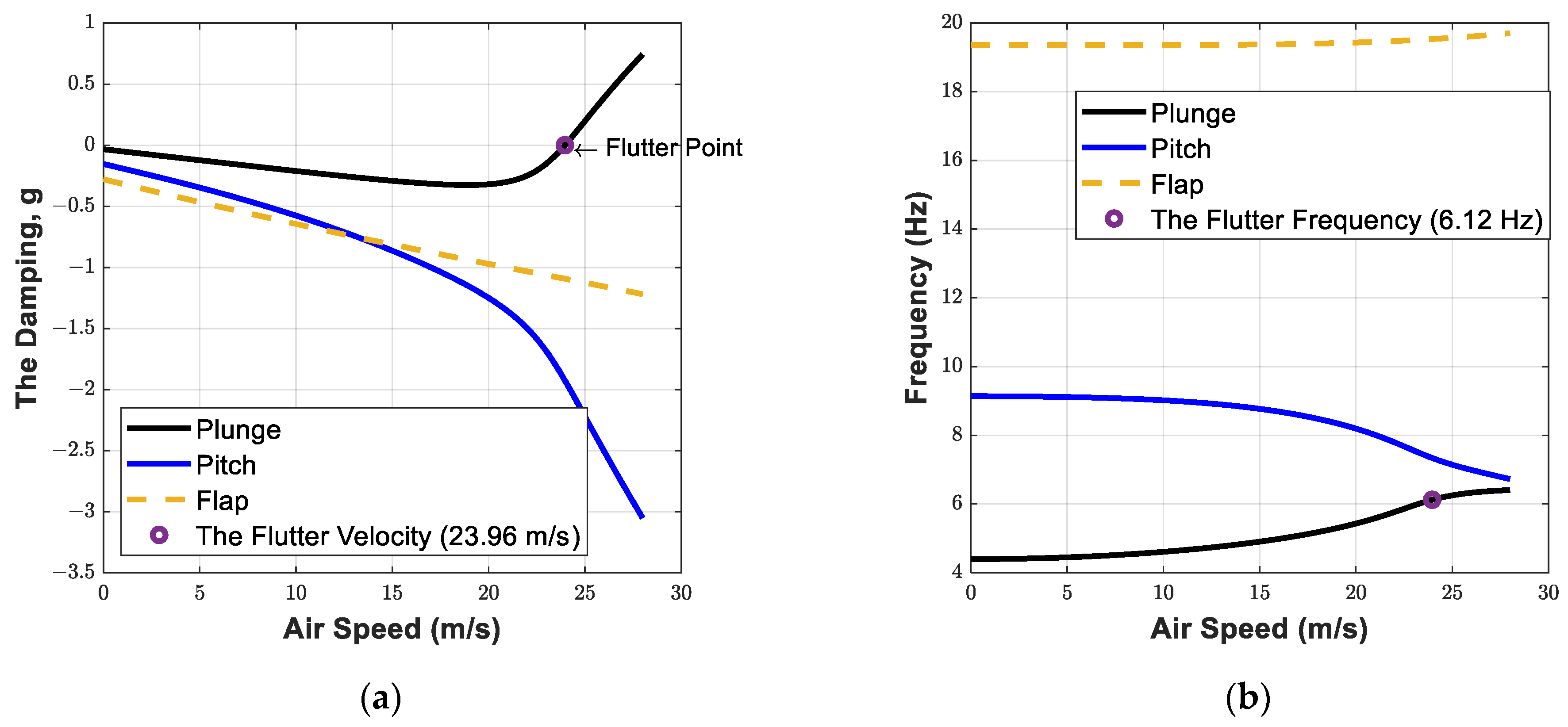
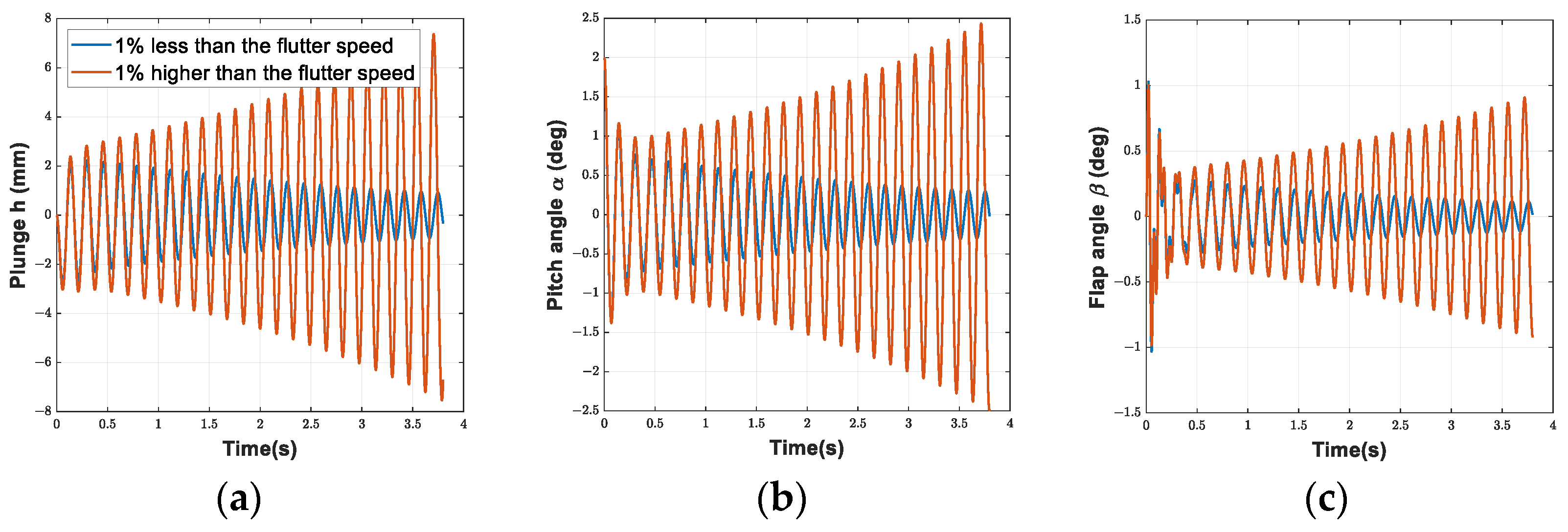
3.1. The Open Loop System Analysis

To validate the model, the system parameters used by Conner et al. [41] and listed in Appendix C were used in this work.

Using the eigenvalue analysis of the state-space model with a constant air density (1.225 kg/m³), as shown in Figure 3, the linear instability (flutter speed) was found to be 23.96 m/s at a frequency of 6.12 Hz.

Figure 3a shows that the damping of both pitch and plunge modes initially increases (in the negative direction), but at some point, the damping of the pitch mode continues to increase, while the damping of the plunge mode begins to decrease and becomes zero at the flutter speed of 23.96 m/s. After this critical speed, the plunge damping becomes positive [42].

Flutter is the result of a combination of at least two modes. This can be seen in Figure 3b, where the pitch and plunge frequencies (the imaginary parts of the eigenvalues) begin to approach each other near the flutter speed without coalescence. At this point, the mode shapes are similar enough to allow energy exchange between them. The pitch mode loses energy to the plunge mode, which is why the pitch mode is highly damped (high negative real part) and the plunge mode is undamped (zero real part) [33,43].

These results are within 15% difference when compared with the experimental work of Conner et al. [41], where the experimental flutter speed was 20.6 m/s at 5.47 Hz. However, they are in exact agreement with the numerical simulation results of the same work. In the author’s opinion, this error is most likely due to the aerodynamic effects not modeled by Theodorsen’s model, as well as the three-dimensional aerodynamic effects in the wind tunnel.

The results in Figure 3b also indicate that the degree of freedom of the control surface has no effect on flutter, which means that a wing system with two degrees of freedom and coalescence between the plunge and pitch modes would lead to the same results. This can be explained by comparing the uncoupled natural frequencies of the studied model: ${\omega }_h=\sqrt{k_h/m}=42.42 \mathrm{rad}/\mathrm{s}$, which is very close to ${\omega }_{\alpha }=\sqrt{k_{\alpha }/I_{\alpha }}=52.65 \mathrm{rad}/\mathrm{s}$, while the flap natural frequency is much higher ${\omega }_{\beta }=\sqrt{k_{\beta }/I_{\beta }}=109.3 \mathrm{rad}/\mathrm{s}$.

To compare the open-loop response of the linear system to an initial disturbance before and after the critical linear flutter speed, the response of the system to the initial condition (2° pitch-angle disturbance) was simulated in the time domain at 1% less and 1% more than the calculated flutter speed. The results are shown in Figure 4.

Figure 4 demonstrates that the generated oscillation of the plunge, pitch, and flap angle asymptotically approaches zero after a few seconds at speeds lower than the critical flutter speed. The aeroelastic system is stable as a result. The oscillations increase infinitely with increasing time at a speed just a little bit over the critical flutter speed. In other words, a tiny unintentional perturbation of the airfoil might act as a catalyst for a severe oscillation. Real physical systems could experience wing separation or damage because of this.

3.2. Closed Loop MPC Using Laguerre Functions

In this section, the discrete-time MPC using Laguerre Functions described in Section 2.2 is designed and tuned to stabilize the wing system in the linear flutter instability region. The calculated optimal controller trajectory is a function of the discrete system matrix ${\mathrm{A}}_m$, which has a different element value at each value of free-stream velocity and air density. For simulation purposes, the airspeed of 25.16 m/s and density of 1.225 kg/m³ (5% above the flutter critical speed) were chosen, and the closed-loop response of the system to the initial disturbance, in addition to the response to step input, were simulated at this speed.

Equation (20) indicates that the LMPC control trajectory $\Delta u$ is a function of the set of discrete-time Laguerre functions $L_i\left(k\right)$, which in turn depend on the choice of the pole of the discrete-time Laguerre network $a$ and the order of the Laguerre network $N$. In addition, $\Delta u$ is a function of $\eta$, calculated from the cost function $J$ shown in Equation (21) and depends on the selection of the weighting matrices $Q$ and $R$. These controller tuning parameters were obtained by trial and error with $N_P=500$, $a=0.3$, $N=16$, $Q=C^{\prime }C$, $R=25,$ and the control horizon for classic MPC was chosen as $N_c=30$. For more details on the influence of the MPC and LMPC parameters on the controller performance, see Refs. [29,37].

Table 1. The closed-loop unconstrained and constrained LMPC system responses to initial conditions (disturbance).

Trial No.	R	u(deg) Input Const.	du/dt Input Const.	Ts for h	ISE for h	Ts for α	ISE for α	Ts for β	ISE for β	ISU	u(deg) max.	du/dt max.
1	25	No	No	0.6	0.02	0.7	0.02	0.5	0.16	0.14	11.8	2000
2	50	No	No	0.8	0.03	0.8	0.02	0.6	0.17	0.15	7.9	1194
3	25	10	105	0.8	0.03	0.8	0.02	0.7	0.13	0.16	3.9	105
4	50	10	105	0.8	0.03	0.8	0.02	0.8	0.14	0.16	3.7	105

shows the closed-loop response of the system to the initial conditions (disturbance) of the unconstrained LMPC in trials 1 and 2 compared to the constrained LMPC in trials 3 and 4 for the same values of tuning parameters. The input constraints must be chosen lower than the physical limits of the actuator to avoid saturation and performance deterioration. For the simulation purpose in this work, the limits were set to $-10°\le u\le 10°, \mathrm{and} -105°/\mathrm{s}\le \frac{du}{dt}\le 105°/\mathrm{s}$.

From Table 1, although the performance is theoretically better when the value of the control cost $R$ is less (more aggressive control input), the control input rate in trials 1 and 2 is too high when compared with the physical limits of an experimental actuator, such as the one reported in Ref. [19], where the dynamics of the motor are neglected, but the maximum deflection of the control surface is reported to be ± 32° and the maximum velocity is only 4.75 rad/s (272 deg/s); this makes trials 1 and 2 impractical. In trials 3 and 4, the effect of the control cost R is less significant in the presence of the controller-imbedded input constraints, as the values of ISE, the settling time, and the ISU are almost similar for the three position states $h, \alpha ,$ and $\beta$.

The position and speed states of the constrained classical MPC and constrained LMPC closed-loop system response to an initial disturbance of 2° pitch angle are shown in Figure 5, and the constrained input with its rate of change are shown in Figure 6. From Figure 6, the rate of change of the input signal cannot exceed the set constraint of 105 deg/s. Limiting the input signal or its rate of change to a certain constraint value such as shown in Figure 6 would be a problem if the control input were calculated offline, as in traditional optimal control methods, but with MPC, the controller measures the output and recalculates the input trajectory at each time step, based only on current states and independent of history.

Figure 5 shows that the system states were successfully and very quickly driven to zero in less than one second with both controllers. Although the final system response is almost the same, the elapsed time required to calculate the control trajectory with the classical MPC was estimated using tictoc function in MATLAB^® environment. The result was 311 milliseconds, while for the LMPC it was 56 milliseconds (82% less). The used hardware was a DELL Inspiron 5559 laptop made by Dell Inc. in China, with Intel^® Core™ i7-6500U CPU at 2.50 GHz microprocessor, and 16 GB of RAM, while the software was MATLAB^® version R2021a from The MathWorks, Inc., Natick, MA, USA, installed over MS Windows 10 Home, version 21H2 operating system from Microsoft Corporation, Redmond, WA, USA. This result suggests that LMPC can be used in place of classical MPC to achieve very similar performance with much less computing power.

In addition, the closed loop system response of the LMPC to a step input of 5° flap angle was tested in the linear flutter instability region, using the same selection of tuning parameters as described above. The results are shown in

Table 2. The closed-loop unconstrained and constrained LMPC system response to step input.

Trial No.	R	u(deg) Input Const.	du/dt Input Const.	ISE for β	Tr	P.O. %	Ts	ISU	u(deg) max.	du/dt max.
1	25	No	No	0.04	0.08	21	0.46	0.17	7.6	332
2	50	No	No	0.04	0.08	19	0.47	0.17	7.5	263
3	25	10	105	0.05	0.09	20	0.47	0.18	7.6	105
4	50	10	105	0.06	0.09	18	0.48	0.18	7.5	105

, Figure 7 and Figure 8 below. As shown, the response is very fast and stable with a settling time of less than 0.5 s and less than 20% overshoot.

4. Conclusions

The objective of this work was to investigate the effectiveness of using discrete LMPC in suppressing the flutter of a two-dimensional wing with a control surface (flap). A mathematical state-space model for a two-dimensional wing with a flap under unsteady aerodynamics was derived and used to determine the linear flutter speed and frequency of an experimental wing. A discrete-time LMPC with Kalman filter for states estimation was then designed, tuned, and quantitatively analyzed for response to initial condition and step input with and without input constraints. The results indicate that the feature of systematic dealing with input constraints is very powerful and useful to avoid actuator saturation and performance deterioration.

To investigate the advantages of LMPC over classical MPC in fast aeroelastic applications that requires powerful computer hardware, the elapsed time required to compute the control trajectory was measured for classical MPC compared to LMPC using tictoc function in the MATLAB environment. The result showed a time saving of 82% when using LMPC, making it a very powerful approach to reduce the required computing power.

References

1. Hodges, D.H.; Pierce, G.A. Introduction to Structural Dynamics and Aeroelasticity, 2nd ed.; Cambridge University Press: Cambridge, UK, 2011. [Google Scholar] [CrossRef]
2. De Marqui, C.; Belo, E.M.; Marques, F.D. A flutter suppression active controller. Proc. Inst. Mech. Eng. Part G J. Aerosp. Eng. 2005, 219, 19–33. [Google Scholar] [CrossRef]
3. Junior, C.D.M.; Rebolho, D.C.; Belo, E.M.; Marques, F.D. Identification of flutter parameters for a wing model. J. Braz. Soc. Mech. Sci. Eng. 2006, 28, 339–346. [Google Scholar] [CrossRef]
4. Kehoe, M.W. A Historical Overview of Flight Flutter Testing. In AGARD Structural and Materials Panel Meeting; NASA-TM-4720; NASA: Washington, DC, USA, 1995. [Google Scholar]
5. Alizadeh, A.; Ebrahimi, Z.; Mazidi, A.; Fazelzadeh, S.A. Experimental nonlinear flutter analysis of a cantilever wing/store. Int. J. Struct. Stab. Dyn. 2020, 20, 2050082. [Google Scholar] [CrossRef]
6. Chen, X.; Hu, R.; Tang, H.; Li, Y.; Yu, E.; Wang, L. Flutter stability of a long-span suspension bridge during erection in mountainous areas. Int. J. Struct. Stab. Dyn. 2020, 20, 2050102. [Google Scholar] [CrossRef]
7. Borglund, D.; Kuttenkeuler, J. Active wing flutter suppression using a trailing edge flap. J. Fluids Struct. 2002, 16, 271–294. [Google Scholar] [CrossRef]
8. Theis, J.; Pfifer, H.; Seiler, P.J. Robust Control Design for Active Flutter Suppression. In Proceedings of the AIAA Atmospheric Flight Mechanics Conference, San Diego, CA, USA, 4–8 January 2016. [Google Scholar]
9. Cunha-Filho, A.; de Lima, A.; Donadon, M.; Leão, L. Flutter suppression of plates using passive constrained viscoelastic layers. Mech. Syst. Signal Process. 2016, 79, 99–111. [Google Scholar] [CrossRef]
10. York, D.L. Analysis of Flutter and Flutter Suppression via an Energy Method. Master’s Thesis, Virginia Tech, Blacksburg, VA, USA, 1980. Available online: https://vtechworks.lib.vt.edu/handle/10919/43300 (accessed on 7 August 2020).
11. Yuan, Y.; Yu, P.; Librescu, L.; Marzocca, P. Aeroelasticity of time-delayed feedback control of two-dimensional supersonic lifting surfaces. J. Guid. Control. Dyn. 2004, 27, 795–803. [Google Scholar] [CrossRef]
12. Marzocca, P.; Silva, W.; Librescu, L. Open/Closed-Loop Nonlinear Aeroelasticity for Airfoils via Volterra Series Approach. In Proceedings of the 43rd AIAA/ASME/ASCE/AHS/ASC Structures, Structural Dynamics, and Materials Conference, Denver, CO, USA, 22–25 April 2002. [Google Scholar]
13. Barker, J.M.; Balas, G.J.; Blue, P.A. Gain-Scheduled Linear Fractional Control for Active Flutter Suppression. J. Guid. Control. Dyn. 1999, 22, 507–512. [Google Scholar] [CrossRef]
14. Horikawa, H.; Dowell, E.H. An Elementary Explanation of the Flutter Mechanism with Active Feedback Controls. J. Aircr. 1979, 16, 225–232. [Google Scholar] [CrossRef]
15. Marretta, R.A.; Marino, F. Wing flutter suppression enhancement using a well-suited active control model. Proc. Inst. Mech. Eng. Part G J. Aerosp. Eng. 2007, 221, 441–452. [Google Scholar] [CrossRef]
16. Ashish, T. Modern Control Design with Matlab and Simulink; John Wiley & Sons: Hoboken, NJ, USA, 2002. [Google Scholar]
17. Karpel, M. Design for active flutter suppression and gust alleviation using state-space aeroelastic modeling. J. Aircr. 1982, 19, 221–227. [Google Scholar] [CrossRef]
18. Garrard, W.L.; Liebst, B.S. Active flutter suppression using eigenspace and linear quadratic design techniques. J. Guid. Control. Dyn. 1985, 8, 304–311. [Google Scholar] [CrossRef]
19. Block, J.; Gilliatt, H.; Block, J.; Gilliatt, H. Active Control of an Aeroelastic Structure. In Proceedings of the 35th Aerospace Sciences Meeting and Exhibit, Reston, NV, USA, 6–9 January 1997. [Google Scholar] [CrossRef]
20. Olds, S.D. Modeling and LQR control of a two-dimensional airfoil. Ph.D. Thesis, Virginia Tech, Blacksburg, VA, USA, 1997. Available online: http://hdl.handle.net/10919/36668 (accessed on 7 August 2020).
21. Hopwood, J.W.; Ruskin, B.; Broderick, D.J.; Wei, F.-S. Aeroservoelastic Design and Wind Tunnel Testing using Parameter-Varying Optimal Control and Inertial-Based Sensing. In Proceedings of the AIAA Scitech 2019 Forum, San Diego, CA, USA, 7–11 January 2019. [Google Scholar] [CrossRef]
22. Darabseh, T.T.; Tarabulsi, A.M.; Mourad, A.-H.I. Active Flutter Suppression of a Two-Dimensional Wing using Linear Quadratic Gaussian Optimal Control. Int. J. Struct. Stab. Dyn. 2022. [Google Scholar] [CrossRef]
23. Bhoir, N.; Singh, S.N. Output feedback nonlinear control of an aeroelastic system with unsteady aerodynamics. Aerosp. Sci. Technol. 2004, 8, 195–205. [Google Scholar] [CrossRef]
24. Sutherland, A.N. A Demonstration of Pitch-Plunge Flutter Suppression Using LQG Control. In Proceedings of the 27th International Congress of The Aeronautical Sciences Conference, Nice, France, 19–24 September 2010. [Google Scholar]
25. Boscariol, P.; Gasparetto, A.; Zanotto, V. Active position and vibration control of a flexible links mechanism using model-based predictive control. J. Dyn. Syst. Meas. Control 2010, 132, 014506. [Google Scholar] [CrossRef]
26. Na, M.G. A model predictive controller for the water level of nuclear steam generators. J. Korean Nucl. Soc. 2001, 33, 102–110. [Google Scholar]
27. Pinheiro, T.C.F.; Silveira, A.S. Constrained discrete model predictive control of an arm-manipulator using Laguerre function. Optim. Control Appl. Methods 2020, 42, 160–179. [Google Scholar] [CrossRef]
28. Mayne, D.Q.; Rawlings, J.B.; Rao, C.V.; Scokaert, P.O.M. Constrained model predictive control: Stability and optimality. Automatica 2000, 36, 789–814. [Google Scholar] [CrossRef]
29. Wang, L. Model Predictive Control System Design and Implementation Using MATLAB®; Springer: London, UK, 2009. [Google Scholar] [CrossRef]
30. Chipofya, M.; Lee, D.J.; Chong, K.T. Trajectory Tracking and Stabilization of a Quadrotor Using Model Predictive Control of Laguerre Functions. In Abstract and Applied Analysis; Hindawi Publishing Corporation: London, UK, 2015; Volume 2015, p. 12. [Google Scholar] [CrossRef]
31. Tewari, A. Aeroservoelasticity: Modeling and Control; Springer: New York, NY, USA, 2015. [Google Scholar] [CrossRef]
32. Fung, Y.C. An Introduction to the Theory of Aeroelasticity; Dover Publications: Mineola, NY, USA, 2002. [Google Scholar]
33. Dimitriadis, G. Introduction to Nonlinear Aeroelasticity; John Wiley & Sons: Hoboken, NJ, USA, 2017. [Google Scholar]
34. Sutherland, A.N. A Small Scale Pitch-Plunge Flutter Model for Active Flutter Control Research. In Proceedings of the 26th International Congress of the Aeronautical Sciences including the 8th AIAA Aviation Technology, Integration, and Operations (ATIO) Conference, Anchorage, AK, USA, 14–19 September 2008. [Google Scholar]
35. Theodorsen, T. Report No. 496, general theory of aerodynamic instability and the mechanism of flutter. J. Frankl. Inst. 1935, 219, 766–767. [Google Scholar] [CrossRef]
36. Rossiter, J.A. Model-Based Predictive Control: A Practical Approach; CRC Press: Boca Raton, FL, USA, 2003. [Google Scholar]
37. Wang, L. Discrete Time Model Predictive Control Design Using Laguerre Functions. In Proceedings of the 2001 American Control Conference, Arlington, VA, USA, 25–27 June 2001. [Google Scholar]
38. Hovland, G. Introduction to Kalman Filtering; METR4200—Advanced Control. 2004. Available online: https://www.scribd.com/document/500629483/METR4200-8 (accessed on 10 August 2020).
39. Outanoute, M.; Selmani, A.; Guerbaoui, M.; Ed-dahhak, A.; Lachhab, A.; Bouchikhi, B. Predictive control algorithm using laguerre functions for greenhouse temperature control. Int. J. Control Autom. 2018, 11, 11–20. [Google Scholar]
40. Dorf, R.C.; Bishop, R.H. Modern Control Systems; Pearson Prentice Hall: Hoboken, NJ, USA, 2008. [Google Scholar]
41. Conner, M.; Tang, D.; Dowell, E.; Virgin, L. Nonlinear Behavior of a Typical Airfoil Section with Control Surface Freeplay: A Numerical and Experimental Study. J. Fluids Struct. 1997, 11, 89–109. [Google Scholar] [CrossRef]
42. Prazenica, R.J. Model Predictive Control of a Nonlinear Aeroelastic System Using Reduced-Order Volterra Models. In Proceedings of the AIAA Atmospheric Flight Mechanics Conference, National Harbor, MD, USA, 13–17 January 2014. [Google Scholar]
43. Wright, J.R.; Cooper, J.E. Introduction to Aircraft Aeroelasticity and Loads; John Wiley & Sons: Hoboken, NJ, USA, 2008; Volume 20. [Google Scholar]
Figure 1. A typical two-dimensional airfoil with a flap.
Aerospace 09 00475 g001
Figure 2. MPC with Kalman Filter Block Diagram.
Aerospace 09 00475 g002
Figure 3. The variation with airspeed of: (a) The damping; (b) The oscillation frequencies.
Aerospace 09 00475 g003
Figure 4. The open-loop response of the system to initial conditions before and after the flutter speed: (a) Plunge motion; (b) Pitch angle; (c) Flap angle.
Aerospace 09 00475 g004
Figure 5. Constrained classic MPC versus constrained LMPC- response to initial disturbance.
Aerospace 09 00475 g005
Figure 6. Constrained classic MPC versus constrained LMPC- input signal and its rate of change.
Aerospace 09 00475 g006
Figure 7. Constrained LMPC response to step input—the output signal.
Aerospace 09 00475 g007
Figure 8. Constrained LMPC response to step input—the input signal and the input rate of change.
Aerospace 09 00475 g008