Three-Dimensional Path Planning for Unmanned Helicopter Using Memory-Enhanced Dueling Deep Q Network

Abstract

Unmanned helicopter (UH) is often utilized for raid missions because it can evade radar detection by flying at ultra-low altitudes. Path planning is the key technology to realizing the autonomous action of UH. On the one hand, the dynamically changing radar coverage area and the mountains in the low airspace environment will seriously affect the flight safety of UH. On the other hand, the huge state space of the three-dimensional (3D) environment will also make traditional algorithms difficult to converge. To address the above problems, a memory-enhanced dueling deep Q-network (ME-dueling DQN) algorithm was proposed. First, a comprehensive reward function was designed, which can guide the algorithm to converge quickly and effectively improve the sparse reward problem. Then, we introduced a dual memory pool structure and proposed a memory-enhanced mechanism, which can reduce invalid exploration, further improve the learning efficiency of the algorithm, and make the algorithm more stable. Finally, the path planning ability of the proposed algorithm in multiple experimental environments was verified. Experiments showed that the proposed algorithm has good environmental adaptability and can help UH to accurately identify dangerous areas and plan a safe and reliable flight path.

1. Introduction

Compared with unmanned aerial vehicle (UAV), unmanned helicopter (UH) has lower requirements for airports and can take off and land in harsh environments [1]. Therefore, they play an important role in the battlefield. The distinctive feature of UH is its strong maneuverability and good concealment, and it can evade radar detection by flying at ultra-low altitudes, thereby raiding important targets [2]. Path planning technology is the basis for UH to safely reach the mission area. Therefore, it is of great significance to study the path planning of UH.

When UH performs raid missions in the low airspace, it will face a very complex airspace environment. First, mountains are a common static obstacle in low-airspace environments, and UH needs to maneuver to avoid mountains to prevent collisions. Then, due to factors such as the curvature of the earth and ground debris, the radar’s detection ability will attenuate with altitude in low airspace [3]. In order to avoid radar detection, UH needs to fly at a low altitude for a long time. Since the probability of UH being detected by radar varies with the flight altitude, it is also difficult to accurately identify the radar area and avoid passing. Finally, the location of the vehicle radar can change at any time, and the coverage area of the radar will become highly dynamic, which also seriously threatens the safety of UH. The purpose of this paper is to seek a reliable path planning scheme to help UH to plan the optimal flight path in a complex dynamic environment.

Existing path planning research is usually conducted in a 2D environment [4]. Since the cruising altitude of the UAV is usually fixed, the dimension of height can be ignored in the path planning research, and only the movement in the horizontal direction is considered. Considering that when UH performs raid missions in low airspace, the flight altitude will also change, and the dimension of flight altitude cannot be ignored. Therefore, it is very necessary to study the path planning of UH in a 3D environment. In previous work, the research on path planning in a 3D environment has also been addressed by related scholars [5,6,7,8]. However, most of these studies were carried out under simple environmental constraints, considering only static environmental constraints, but not highly dynamic complex environmental constraints.

The salient feature of the three-dimensional environment compared with the two-dimensional environment is that it has a huge state space, which brings a great burden to the algorithm for path search. Commonly used path planning algorithms such as the Dijkstra algorithm, A* algorithm, particle swarm algorithm, ant colony algorithm, genetic algorithm, and artificial potential field method all require a lot of calculations in the path search [9,10,11,12], so the application of these algorithms in the 3D environment is very limited.

Deep reinforcement learning technology is produced by the combination of reinforcement learning and deep learning, which inherits the ability of reinforcement learning to interact with the environment autonomously and the powerful state representation ability of deep learning [13]. The application ability of deep reinforcement learning technology in large state space has been proved by related research [14]. Therefore, using deep reinforcement learning techniques for path planning in 3D environments has significant advantages. First of all, deep reinforcement learning can dynamically adjust parameters by interacting with the environment independently, so as to find the optimal strategy, and this process does not require tedious operations. Second, deep reinforcement learning can store learning information through neural networks, and there is no state space explosion problem when processing large state space information. Finally, deep reinforcement learning is less dependent on prior knowledge of the environment, and has stronger adaptability to dynamic environments.

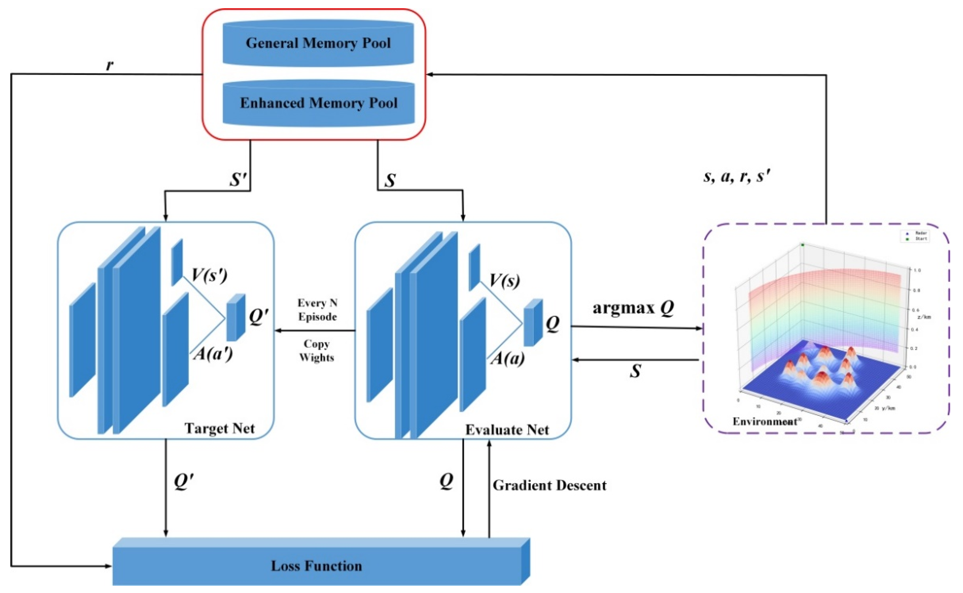
In this paper, a memory-enhanced dueling deep Q-network (ME-dueling DQN) algorithm is proposed, and it is embedded into the UH performing low-altitude raid mission model for path planning. Experimental results show that the proposed algorithm can converge quickly and plan a safe and effective flight path for UH in complex dynamic environments. The main contributions of this paper are as follows:

(1) Combined with the environment model, a comprehensive reward function is designed. On the basis of improving the sparse reward problem, the planning path is further optimized, and the convergence speed of the algorithm is improved.

(2) A memory-enhanced mechanism is proposed. The dual experience pool structure is introduced into the traditional dueling deep Q network structure, and the learning efficiency of the algorithm is improved by the memory-enhanced mechanism, making the learning process of the algorithm more stable.

(3) A three-dimensional environment model of UH’s raid missions in the low airspace is established. The whole process of embedding the proposed algorithm into the environment model to realize path planning is introduced in detail, and a new solution to the path planning problem is provided.

In general, this paper attempts to use deep reinforcement learning algorithms to solve the path planning problem in complex dynamic environments, which has certain significance for related research. First, the definition process of the reward function can be used for reference by related scholars. Then, the proposed memory-enhancing mechanism can also be extended to more general intelligent algorithms. Finally, the problem of path planning in complex 3D environments is relatively understudied, and this paper can enrich case studies in this area.

The remainder of this paper is structured as follows: Section 2 presents related work. The establishment of the 3D environment model is introduced in Section 3. Section 4 introduces reinforcement learning theory and the traditional Dueling DQN algorithm. The details of the proposed algorithm and the implementation of path planning are presented in detail in Section 5. Section 6 presents the implementation results and discusses them. Section 7 is the conclusion of this paper.

2. Related Works

Path planning refers to finding the optimal path from the starting point to the endpoint according to certain constraints [15]. Usually, there are many feasible paths from the starting point to the endpoint, but the optimal path can be selected according to some criteria, such as the shortest distance, the straightest path, and the least energy consumption [16]. Path planning can be divided into three parts: establishing an environment model, path search, and path generation [17]. In these works, establishing an environment model is the basis of path planning, path search is the core work, and path generation is the presentation of the final planning results.

For a long time, the path search algorithm has been the focus of path planning research. The path search algorithm can be divided into a global path search algorithm and a local path search algorithm according to the situation of obtaining environmental information [18]. In the global path search algorithm, the information of the environment model is required to be completely known, and the algorithm can quickly search for the optimal path based on this information. However, it is usually difficult to obtain complete environmental information, so the application of the global path search algorithm is relatively limited. Because the local path search algorithm can explore the optimal path based on limited environmental information, it has received more extensive attention [19]. The reinforcement learning algorithm is a typical local path planning algorithm.

Path planning has always been a research hotspot in various fields. In [20], the authors used the A* algorithm to generate a global path for UAVs, and then used the path results as input for task assignment, which improved the overall performance of UAV mission planning. An online path re-planning algorithm for autonomous underwater vehicles was proposed in [21], where the authors used particle swarm optimization together with a cost function to enable the algorithm to operate efficiently in a cluttered and uncertain environment. A new hybrid algorithm for UAV 3D environment path planning was proposed in [22], which combined metaheuristic ant colony algorithm and differential evolution algorithm to form a new path planning method, and had strong robustness and fast convergence. In [23], a new genetic algorithm based on a probability graph was proposed, the author completed the path planning of the UAV by introducing a new genetic operator to select appropriate chromosomes for crossover operation. An improved artificial potential field algorithm for motion planning and navigation of autonomous grain carts was proposed in [24], which combined an artificial potential field algorithm and fuzzy logic control to improve the robustness and work efficiency of the algorithm. It is worth noting that these traditional algorithms search for paths based on real-time environmental information. If the environmental information changes, the planned path obtained in this way has a certain lag and may not fully meet the needs. Therefore, the above-mentioned traditional algorithms are difficult to adapt to the complex and dynamic low-airspace environment faced by the UH’s mission.

The distinctive feature of reinforcement learning is that the search for the optimal strategy can be completed without prior knowledge. Therefore, the application of reinforcement learning to path planning has certain advantages [25]. With appropriate reward settings, reinforcement learning algorithms can autonomously complete the path search task by interacting with the environment when the environmental information is unknown. A more representative and relatively mature reinforcement learning algorithm is the Q-Learning algorithm.

The application of the Q-Learning algorithm in the path planning problem has been widely studied. In the literature [26], the author transformed environmental constraints such as distance, obstacles, and forbidden areas into rewards or punishments, and proposed a path planning and manipulation method based on the Q-Learning algorithm, which completed the autonomous navigation and control tasks of intelligent ships. A novel collaborative Q-Learning method using the Holonic Multi Agent System (H-MAS) was proposed in [27]. The author used two different Q-tables to improve the traditional Q-Learning to solve the path planning problem of mobile robots in unknown environments. In the literature [28], the author initialized the Q table by designing a reward function to provide the robot with prior knowledge, and designed a new and effective selection strategy for the Q-Learning algorithm, thus completing the task of optimizing the path for a mobile robot in a short time. However, the Q-Learning algorithm needed to constantly update the Q table in the process of working. A large number of operations of reading and storing the Q value greatly reduced the work efficiency of the algorithm, resulting in a very limited ability of the algorithm to deal with a large state space.

Deep reinforcement learning uses neural networks to fit the update process of reinforcement learning algorithms, which greatly enhances the ability of reinforcement learning algorithms to process large state space data. The deep Q network is the product of the combination of the Q-Learning algorithm and the neural network, which can effectively improve the Q-Learning algorithm’s ability to process large state space data while inheriting the advantages of the Q-Learning algorithm [29].

In recent years, many scholars have tried to use the DQN algorithm for path planning. In [30], the authors employed a dense network framework to compute Q-values using deep Q-networks. And according to the different needs for the depth and breadth of experience in different learning stages, they proposed an improved learning strategy, and completed the robot’s navigation and path planning tasks. Aiming at the problem of slow convergence and instability of traditional deep Q-network (DQN) algorithm in autonomous path planning of unmanned surface vehicles, an improved Deep Double-Q Network (IPD3QN) based on Prioritized Experience Replay was proposed in [31]. The author used a deep double-Q network to decouple the selection and calculation of the target Q-value action to eliminate overestimation, and introduced a duel network to further optimize the neural network structure. A probabilistic decision DQN algorithm was proposed in [32]. The authors combined the probabilistic dueling DQN algorithm with a fast active simultaneous localization and map creation framework to achieve autonomous navigation of static and dynamic obstacles of varying numbers and shapes in indoor environments. In [33], the authors proposed ANOA, a deep reinforcement learning method for autonomous navigation and obstacle avoidance of USVs, by customizing the design of state and action spaces combined with a dueling deep Q-network. This algorithm completed the path planning tasks of unmanned surface vehicles in static and dynamic environments. Although the above research has proved the application ability of the DQN algorithm in large state space, its application ability in a highly complex and dynamic battlefield environment still needs to be further studied.

Dueling Deep Q-Network (Dueling DQN) is an improved algorithm of the DQN algorithm. In [34], the author decomposed the model structure of the DQN algorithm into two parts, the state value function (V value) and the advantage function (A value), and proposed Dueling DQN, which made the model training pay more attention to high-reward actions and accelerated the convergence speed. Due to the stronger ability of Dueling DQN to process large state space information and the fast convergence speed, this paper conducts research on UH low-altitude raid path planning based on Dueling DQN.

3. System Model and Problem Definition

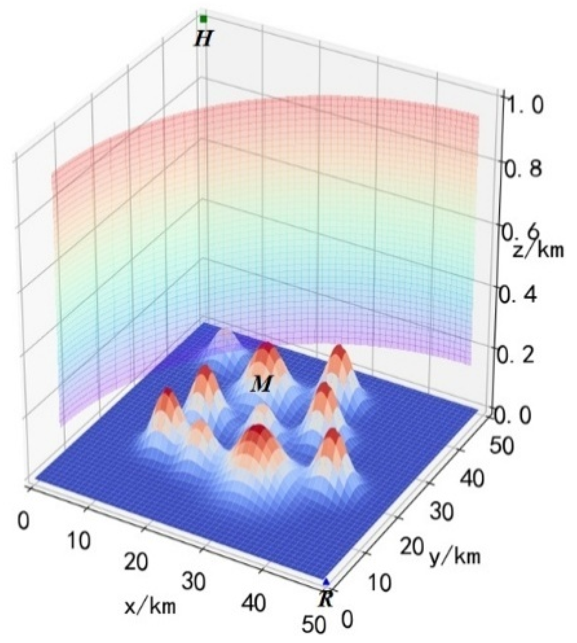
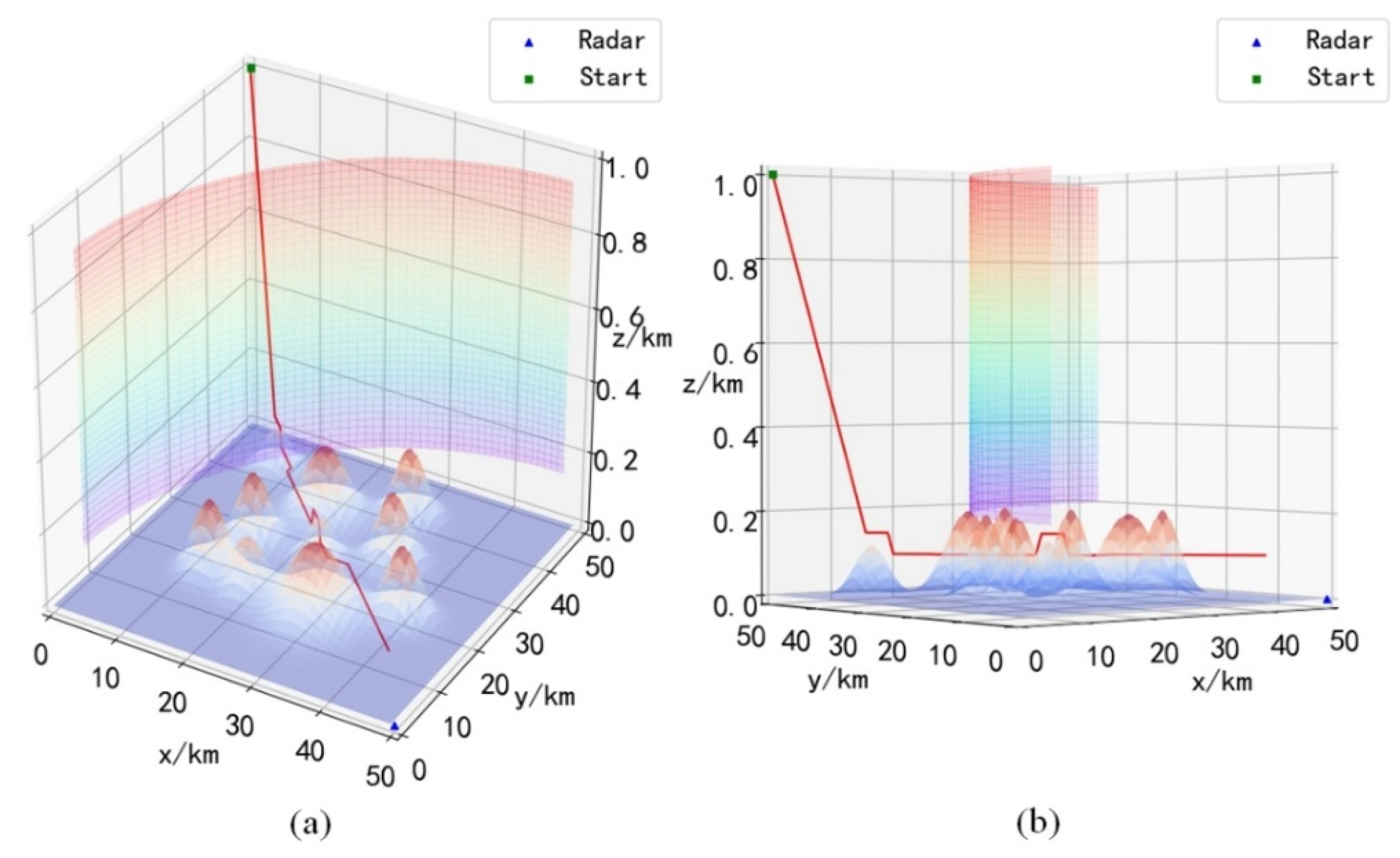
As shown in Figure 1, a 3D battlefield environment $E$ is established, whose length, width and height are 50 km, 50 km, and 1 km, respectively. Unmanned helicopter $H$, mountain range $M$ and radar $R$ are included in the battlefield environment $E$. The $H$ can move freely in $E$, the position of $H$ in $E$ can be expressed as:

$$H_{\left(x,y,z\right)}=\left[x,y,z\right]$$

(1)

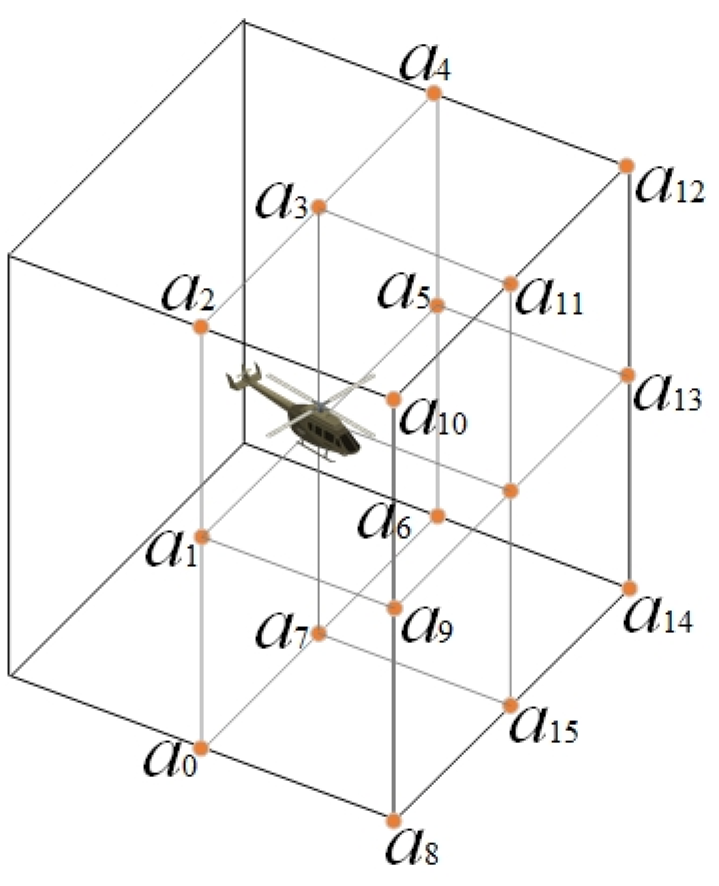
In Equation (1), $H_{\left(x,y,z\right)}$ represents the position of the unmanned helicopter in the battlefield environment. The $H$ has flexible maneuverability, and it can choose to fly straight ahead in the horizontal direction, or choose to turn 45/90 degrees left or right. In the vertical direction, it can choose to climb up 45/90 degrees or descend 45/90 degrees. Then $H$ can move with 17 degrees of freedom in $E$, as shown in Figure 2.

$H$ cannot collide with mountains during flight, that is, the $H$ cannot be contained within the $M$:

$$H_{\left(x,y,z\right)}\notin M$$

(2)

The mountain range $M$ can be determined by the horizontal coordinates $x$ and $y$, and the height of the mountain at the horizontal position $\left(x,y\right)$ can be expressed as:

$$M_{Z\left(x,y\right)}={\sum }_{i=1}^N{h}_i{e}^{-{(\frac{x-a_i}{c_i})}^2-{(\frac{y-b_i}{c_i})}^2}$$

(3)

In Equation (3), $M_{Z\left(x,y\right)}$ is the height of the mountain at horizontal position $\left(x,y\right)$, $h_i$ is the height coefficient, $\left(a_i,b_i\right)$ represents the center position of the mountain range $M$, and $c_i$ can control the size of the mountain range $M$.

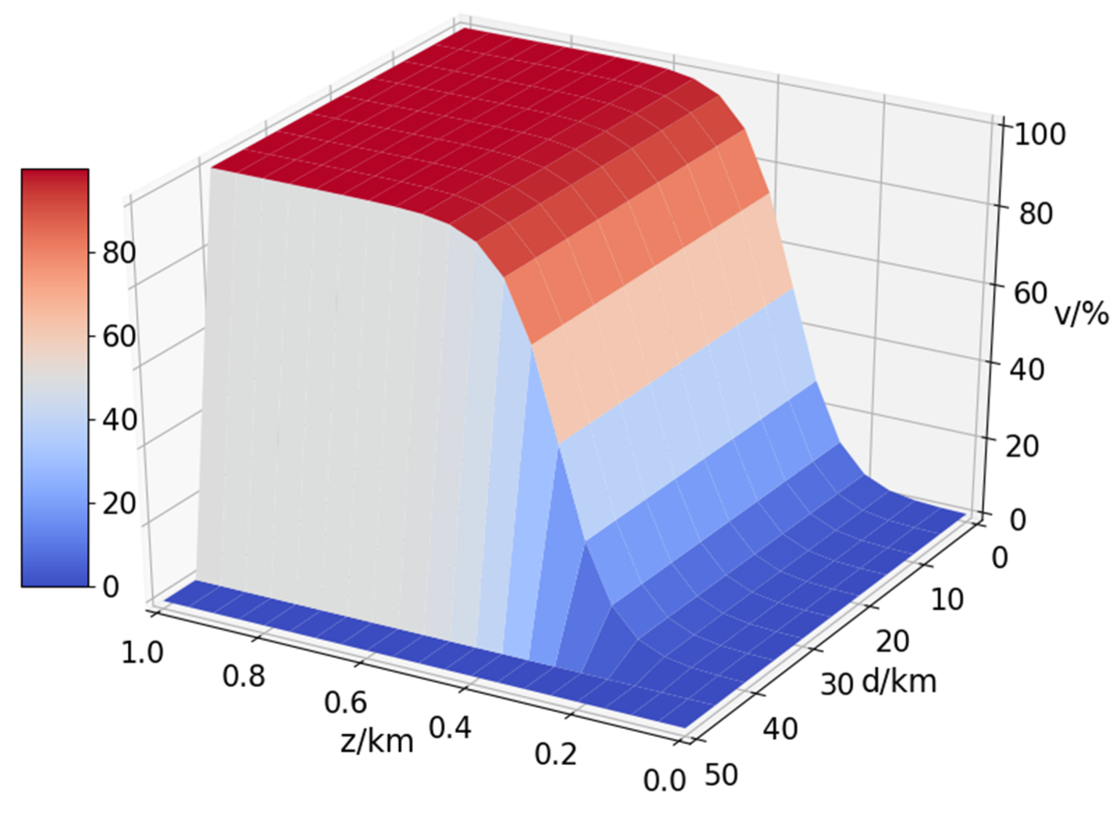
The position of $R$ can be determined by the $\left(x,y,z\right)$ three-dimensional coordinates, but $z$ defaults to 0. Due to the influence of factors such as the curvature of the earth, it is difficult for radar to detect ultra-low-altitude flying targets, and the detection ability of radar will change with altitude. Assuming that the detection distance of the radar is up to 45 km, the radar detection probability formula can be expressed as:

$$v=\left\{\begin{array}{l}0,d>45 \mathrm{km}\\ 1,d\le 45 \mathrm{km},z\ge 1 \mathrm{km}\\ \frac{1}{1+e^{\left(-\left(20h-7\right)\right)}},d\le 45 \mathrm{km},0.2 \mathrm{km}<z<1 \mathrm{km}\\ 0,z\le 0.2 \mathrm{km}\end{array}\right.$$

(4)

In Equation (4), $d$ is the relative distance between the UH and the radar, and $z$ is the flying height of the UH. In order to observe the radar coverage more intuitively, the Equation (4) is drawn as a 3D probability distribution diagram to obtain Figure 3.

In Figure 3, the v-axis is the probability of being detected by the radar. Combining the Equation (4) and Figure 3, it can be seen that when the UH passes through the radar coverage area, the flight height should be less than 0.2 km, and then it can ensure its own absolute safety. When the UH flight altitude $z\in \left(0.2,0.5\right)$, it is not guaranteed to be detected by radar, but this behavior is also dangerous and should be avoided.

The UH’s mission is to raid and destroy the opponent’s radar. The maximum attack range of UH is 8 km, assuming that UH can find it and destroy it. Then the conditions for UH to complete the raid mission are: the relative distance $d_t$ between UH and radar is less than 8 km, which can be expressed as:

$$d_t=\left|H_{\left(x,y,z\right)}-R_{\left(x,y,z\right)}\right|=\sqrt{{(x_H-x_R)}^2+{(y_H-y_R)}^2+{(z_H-z_R)}^2}\le 8\mathrm{km}$$

(5)

In Equation (5), $R_{\left(x,y,z\right)}$ represents the position of the radar. Building a system model is an important step in path planning research. After the above discussion, we modeled and numerically analyzed the battlefield environment for UH to perform raid missions in low airspace, and clarified the environmental constraints and mission objectives. The purpose of this research is to plan a safe and reliable flight path for UH, and the evaluation indicators should be clearly defined to describe the pros and cons of the planned path. First, to ensure the safety of the UH, the planned path cannot collide with mountains and cross the radar coverage area. Then, in order to reduce the flight consumption of UH, the length of the planned path should be as short as possible. Finally, the planned path should be as straight as possible, and the number of turns should be as few as possible, which can further reduce flight consumption.

4. Basic Algorithms

4.1. Traditional Algorithms

For comparison and analysis with our proposed algorithm, we introduce two relatively representative traditional algorithms in this section.

4.1.1. Dijkstra Algorithm

Dijkstra algorithm is a commonly used optimization algorithm for finding the shortest path. The algorithm can effectively solve the shortest path problem from a single starting point to the target point in a directed graph [35]. The flow of Dijkstra algorithm can be expressed as:

(1) Initialize the shortest distance between each point and the starting point. If there is a straight-line path between a certain point $k$ and the starting point $A$, and the distance satisfies the correction constraint, the shortest distance from the point k to the starting point $A$ is the straight-line distance, denoted as $D\left(k,A\right)=j_{kA}$; if there is no straight-line distance between point $k$ and point $A$ to reach, or the distance when reaching this point violates the correction constraint, then initialize the shortest distance from point $k$ to point $A$ to infinity, denoted as $D\left(k,A\right)=+\infty$.

(2) Traverse all points except the end point $T$ in turn, and perform the following operations on each point: first, find the reachable point closest to the point, denoted as $k$, and mark the status of point $k$ as visited; then, traverse $k$ points in turn all points that can be reached in a straight line and have not been visited, denote the point as $l$, and denote $j_{kl}$ as the distance between $k$ and $l$; finally, if $D\left(k,A\right)+j_{kl}<D\left(l,A\right)$, then the shortest distance $D\left(l,A\right)$ from point $l$ to point $A$ is updated to $D\left(k,A\right)+j_{kl}$;

(3) Repeat the above process until the shortest path to all points is found.

4.1.2. A* Algorithm

A* algorithm is a typical heuristic search algorithm established on the basis of the Dijkstra algorithm, and it is also a commonly used effective algorithm for searching the shortest path [36]. The core of A* algorithm is to perform a heuristic evaluation function:

$$f\left(\mathrm{k}\right)=g\left(k\right)+u\left(k\right)$$

(6)

where $f\left(\mathrm{k}\right)$ represents the heuristic function corresponding to the algorithm when searching for any point. $g\left(k\right)$ represents the cost from the starting point to the current point, and $u\left(k\right)$ represents the estimated value of the cost from the current point to the end point. During the execution of the algorithm, the point with the smallest $f\left(\mathrm{k}\right)$ value will always be selected as the next point of the optimal path.

In the process of application, $u\left(k\right)$ is usually taken as the Euclidean distance or Manhattan distance from the current point to the end point. If the value of $u\left(k\right)$ is 0, the A* algorithm will degenerate into the Dijkstra algorithm, the search space of the algorithm will become larger, and the search time will also become longer. Since the execution process of the A* algorithm is similar to that of the Dijkstra algorithm, it will not be repeated here.

4.2. Deep Reinforcement Learning Algorithms

4.2.1. Q-Learning Algorithm

Reinforcement learning is a learning method that maps from state space to action space [37]. The state set $S$, the action set $A$, the state transition probability $P$ and the reward set $R$ are important components of the reinforcement learning model. A policy $\pi :S\to A$ can be defined, which is the mapping from the state set to the action set. First, during the operation of the algorithm, the learner will select the action $a$ according to the policy $\pi$ in the current state $s$. Then, after the action $a$ is executed, the environment will transition to the next state $s\prime$ according to the probability $P$. Finally, the environment will judge the action $a$ according to the reward rules and give the appropriate reward $r$. Since the purpose of reinforcement learning is to maximize the accumulated reward, the algorithm will automatically adjust the strategy according to the reward value during the iteration process. Through the above iterative process, the reinforcement learning algorithm can interact with the environment autonomously to seek the optimal strategy. Q-Learning is a representative reinforcement learning algorithm, and its update method is as follows:

$$Q\left(s,a\right)=Q\left(s,a\right)+\alpha \left(r+\gamma \underset{a^{\prime }}{\max }Q\left(s^{\prime },a^{\prime }\right)-Q\left(s,a\right)\right)$$

(7)

In Equation (7), $\alpha \in \left(0,1\right]$ represents the learning rate, which can control the proportion of future rewards in the learning process. And $\gamma \in \left(0,1\right)$ represents the decay factor, which can control the decay of future rewards. The convergence of Equation (7) has been proved in [38]. However, the Q-Learning algorithm needs to use the Q table to store the Q value corresponding to each action during the running process. On the one hand, the continuous reading and writing of the Q value makes the algorithm update process extremely difficult Slow. On the other hand, the storage capacity of the Q-table is limited, which makes it difficult for the Q-Learning algorithm to handle large state space information.

4.2.2. Deep Q-Network

On the basis of reinforcement learning, the introduction of neural networks to form deep reinforcement learning can effectively improve the above problems. The DQN algorithm uses a neural network to fit the update process of the Q-Learning algorithm:

$$QQ\left(s,a,\omega \right)\approx Q\left(s,a\right)$$

(8)

In Equation (8), $\omega$ represents the neural network parameter. In the working process of the DQN algorithm, the state $s$ is used as the input, and the Q values corresponding to different actions are output. Through this process, the neural network completes the state-to-action mapping work, so it is no longer necessary to generate a Q table to store the Q value information. The DQN algorithm can update the Q value by updating the neural network parameters. The loss function $L\left(\omega \right)$ in the update process is:

$$L\left(\omega \right)=E\left[{\left(r+\gamma \underset{a^{\prime }}{\max }Q\left(s^{\prime },a^{\prime },\omega \right)-Q\left(s,a,\omega \right)\right)}^2\right]$$

(9)

The network parameter $\omega$ is updated using the stochastic gradient descent algorithm, and the update value $\mathsf{\Delta }\omega$ is:

$$\frac{\delta L\left(\omega \right)}{\delta \omega }=\left[r+\left(\gamma \underset{a^{\prime }}{\max }Q\left(s^{\prime },a^{\prime },\omega \right)-Q\left(s,a,\omega \right)\right)\right]\frac{\delta Q\left(s,a,\omega \right)}{\delta \omega }$$

(10)

The success of the DQN algorithm is inseparable from the experience replay mechanism and the target network mechanism [39]. The experience replay mechanism requires the establishment of a memory pool to store past experiences, and then the algorithm randomly selects experience samples from the memory pool for training. On the one hand, the experience replay mechanism can overcome the correlation of empirical data and promote algorithm convergence. On the other hand, the experience replay mechanism can make the algorithm gradient descent move in the same direction, thereby reducing the variance of parameter updates and overcoming the non-stationary distribution problem.

The target network mechanism further promotes the algorithm convergence by introducing a dual network structure (Evaluate Net and Target Net) to solve the problem of strong data dependence when a single network is updated. The parameters of the Target Net and the Evaluate Net are exactly the same. Whenever the algorithm executes a certain number of steps, the parameters of the Evaluate Net will be completely copied to the Target Net. In Equation (9), Q(s, a, ω) is generated by the Evaluate Net, and Q(s’, a’, ω) is generated by the Target Net.

4.2.3. Dueling Deep Q-Network

Dueling DQN is an improved algorithm based on DQN by optimizing the neural network structure [40]. The neural network of the traditional DQN algorithm will directly output the Q value corresponding to each action, and then select the optimal action. The output layer of the neural network of the Dueling DQN algorithm is divided into two parts: the state value function $V\left(s\right)$ and the action advantage function $A\left(a\right)$. Among them, the state value function $V\left(s\right)$ represents the value of the static state environment itself, and the action advantage function $A\left(a\right)$ represents the additional value brought by choosing an action. Finally, the two functions are aggregated to obtain the Q value corresponding to each action:

$$Q\left(s,a,\omega ,{\omega }_V,{\omega }_A\right)=V\left(s,\omega ,{\omega }_V\right)+A\left(s,a,\omega ,{\omega }_A\right)$$

(11)

In Equation (11), ω is the parameter of the common part of the neural network, ${\omega }_V$ and ${\omega }_A$ respectively represent the unique neural network parameters of the state value function $V\left(s\right)$ and the action advantage function $A\left(a\right)$. In order to more clearly express the respective roles of $V\left(s\right)$ and $A\left(a\right)$, Equation (11) can be turned into another form:

$$Q\left(s,a,\omega ,{\omega }_V,{\omega }_A\right)=V\left(s,\omega ,{\omega }_V\right)+\left(A\left(s,a,\omega ,{\omega }_A\right)-\frac{1}{\left|\mathrm{A}\right|}{\sum }_{a\prime }A(s,a\prime ,\omega ,{\omega }_A)\right)$$

(12)

Equation (12) is the centralized processing of the advantage function, which can further improve the stability of the network. The advantage of the Dueling DQN algorithm is that it can learn the $V\left(s\right)$ value of each state without considering what action to take in this state, which can effectively improve the learning efficiency.

5. Path Planning Using Memory-Enhanced Dueling Deep Q Network

5.1. Divide State Set and Action set

The division of state set and action set is the basic link of path planning using reinforcement learning algorithms. Since the state space is required to be discrete when using the Dueling DQN algorithm for path planning, the environment model needs to be discretized. The grid method is a commonly used discretization method [41]. The battlefield environment $E$ can be discretized into $2\times {10}^5$ cubes of equal size with the help of a $100\times 100\times 20$ three-dimensional grid. For ease of calculation, it is assumed that the UH stays at the intersection of the grid after each action. Since the length, width, and height of the battlefield environment are 50 km, 50 km, and 1 km, respectively, after discretization, UH moving one grid in the horizontal direction means flying 0.5 km, and moving one grid in the vertical direction means flying 0.05 km. After the above operations, the flight path of the UH is discretized into a series of three-dimensional coordinate points. The state set can be divided according to the total position of UH in the environment as the input of the algorithm:

$$s_i=\left[x_H,y_H,z_H\right],s_i\in S,i\in \left[1,2\times {10}^5\right]$$

(13)

It can be seen from Equation (13) that the environment $E$ is divided into $2\times {10}^5$ states. For such large state space information, traditional reinforcement learning algorithms are difficult to handle, which is an important reason why we use deep reinforcement learning for UH path planning.

Since each action of UH must be moved according to the action constraints, the division of action set should also be carried out according to the action set of UH. As can be seen from Section 3, UH can move in 17 directions in the battlefield environment, then the action set is divided into:

$$a_i\in A,i\in \left[0,17\right]$$

(14)

In Equation (14), $a_i$ is consistent with Figure 2.

5.2. Design a Comprehensive Reward Function

Setting an appropriate reward function is the key to the smooth convergence of reinforcement learning algorithms. In the commonly used reward rules, learners can only get reward value when they complete the task, and a series of behaviors before completing the task will not be rewarded in time. This reward method will cause the algorithm to fail to get timely feedback and thus have difficulty in convergence, which is the so-called sparse reward problem [42]. Since the state set divided by the battlefield environment $E_{\left(x,y,z\right)}$ is large, it is unrealistic to use the traditional reward rules to converge the algorithm. In order to enable the algorithm to plan a safe path smoothly, we design a comprehensive reward function based on the environment model. The reward function mainly includes three parts: guidance reward, straightness reward, and incentive reward.

5.2.1. Guidance Reward

In order to enable the algorithm to get timely feedback from the environment, we design a guidance reward $r_1$, which is expressed in the following form:

$$r_1=d_t-d_{t+1}$$

(15)

In Equation (15), $d_t$ represents the relative distance between the current position UH and the raid target, and $d_{t+1}$ represents the relative distance between the next position UH moves to after taking action $a_t$ and the raid target. It can be seen from the formula that whenever UH takes an action, if it is closer to the task goal ($d_t>d_{t+1}$), the action $a_t$ will get a positive reward, if it is further away from the task goal ($d_t<d_{t+1}$), the action $a_t$ will be punished. The value of reward and punishment in the formula will also change with the degree of UH’s approach to the principle target, which can more accurately describe the pros and cons of action $a_t$, so that the accumulation of rewards is smoother. The guidance reward $r_1$ allows the algorithm to get timely feedback after each action of UH, so as to accurately determine whether taking the corresponding action $a_i$ in the state $s_i$ is conducive to the completion of the task, which can effectively improve the sparse reward problem. The guidance reward uses the task target as the guide factor to prompt the algorithm to choose actions that are beneficial to the UH approaching the target as much as possible, which further promotes the interaction between the algorithm and the environment, and can effectively speed up the algorithm convergence.

5.2.2. Straightness Reward

In the process of UH flight, the constant change of flight direction will speed up the consumption of fuel and increase the flight risk. In order to make the planned path straighter and further ensure flight safety, we design a straightness reward $r_2$:

$$r_2=\left\{\begin{array}{l}-\theta {\left|d_t-d_{t+1}\right|}_{max},if{a}_t\ne a_{t+1}\\ 0,else\end{array}\right.$$

(16)

In Equation (16), $\theta$ is a positive constant representing the straightness coefficient, and ${\left|d_t-d_{t+1}\right|}_{max}$ represents the maximum distance of one movement of UH. The role of the straightness reward $r_2$ is mainly to punish the UH’s turning behavior. $r_2$ can further constrain the behavior of UH and minimize the selection of turning behaviors, thereby making the planned path. Of course, our ultimate goal is not to make the planned path a continuous curve with no turns at all, which will make UH lose its ability to avoid obstacles. The introduction of $r_2$ only restricts the corner behavior to a certain extent, thereby reducing the meaningless turning behavior and further reducing the risk of UH collision. Therefore, $\theta$ needs to take an appropriate value, which can not only reduce the turning of the planned path, but also will not affect the obstacle avoidance ability of UH. The value of $\theta$ will be analyzed in the experimental part.

5.2.3. Incentive Reward

The guidance reward promotes algorithm convergence, and the straightness reward further optimizes the planned path, but they all take effect when the UH is not in danger. In order to ensure the safety of UH, we design the incentive reward $r_3$:

$$r_3=\left\{\begin{array}{l}-10{\left|d_t-d_{t+1}\right|}_{max},if crash\\ 10{\left|d_t-d_{t+1}\right|}_{max},if win\end{array}\right.$$

(17)

The value of $r_3$ is much larger than $r_1$ and $r_2$, because we want to motivate UH to complete the task as much as possible while ensuring its own safety. It is strictly forbidden to crash (hit a mountain or be detected by radar) as a serious threat to flight safety, so severe punishment should be given. When UH completes the raid, it deserves to be heavily rewarded. The incentive reward is the key to enabling the algorithm to accurately identify threat areas. In the process of interacting with the environment, the algorithm can explore the radar coverage area according to the incentive reward, so as to avoid crossing. It is worth noting that when the incentive reward $r_3$ takes effect, it means that the UH has crashed or the mission has been completed, then the system will restart and perform a new round of training.

5.2.4. Comprehensive Reward Function

The comprehensive reward function $R_c$ is obtained by summarizing the rewards of each part, and its specific form is:

$$R_c=r_1+r_2+r_3$$

(18)

Combined with the above analysis, it can be seen that the comprehensive reward function can effectively combine the environmental information to give the algorithm feedback in time, and further optimize the planning path while promoting the algorithm convergence. And the comprehensive reward function effectively converts environmental constraints and action constraints into reward rules, so that the deep reinforcement learning algorithm can further perceive environmental information, interact with the environment smoothly, and seek optimal strategies. Therefore, the setting of the comprehensive reward function is an important prerequisite for the algorithm to perform path search.

5.3. Memory-Enhanced Mechanism

In the traditional Dueling DQN algorithm, our experience replay mechanism is to randomly sample and learn all past experiences. Although this method can improve the learning efficiency, it is not efficient, because the past experience is not all able to promote the convergence of the algorithm. Although some scholars have proposed a priority experience playback mechanism to improve this problem, the priority replay mechanism also has problems such as cumbersome construction and low operating efficiency, which can easily cause the algorithm to converge in an irrational direction [43]. In order to further promote the convergence of the algorithm and improve the efficiency of sampling learning, a memory-enhanced mechanism is designed on the basis of retaining the original experience replay mechanism. The core idea of the memory-enhanced mechanism is to perform multiple sampling learning from enhanced memory to improve learning efficiency. Enhanced memory refers to those memories that make a deep impression on UH during exercise, such as crashing or completing a task (receiving a strong punishment or reward). As well, enhanced memory pool is built to store these memories individually. Whenever the UH crashes again or completes the task, the enhanced memory pool will be sampled and learned by random sampling. Then, in other cases, sample learning is still performed on all memories. The specific working process of the memory-enhanced mechanism will be further explained in the next subsection.

Introducing a memory-enhanced mechanism has the following benefits. First of all, it can effectively reduce the occurrence of crash events in the early stage of the algorithm running process, and promote the rapid convergence of the algorithm. Because the UH will sample and learn from the enhanced memory pool every time it crashes, it will reinforce its memory of the crash event, so that it can learn to avoid danger faster. Secondly, it can reinforce the memory of completing the task in the later stage of the algorithm operation, thereby improving the success rate of UH completing the task and making the algorithm converge more stably. The proposal of the memory-enhanced mechanism is inspired by the human learning process. Impressive things are always quicker to comprehend and lasting unforgettable for humans, the memory-enhanced mechanism we designed also complies with this, which can further improve the performance of the algorithm.

5.4. Memory-Enhanced Dueling Deep Q-Network

Path search is the key link to completing the path planning task. There are significant advantages to using the ME-Dueling DQN algorithm for path search. First, the ME-Dueling DQN algorithm can complete the path search task without prior knowledge, and can well adapt to unknown environmental models. Then, the ME-Dueling DQN algorithm has strong data processing ability and can better handle the large state space of the 3D environment. Finally, the convergence of the ME-Dueling DQN algorithm can be guaranteed under appropriate reward settings. The ME-Dueling DQN algorithm model is shown in the Figure 4.

Figure 4. shows the path planning process of the ME-Dueling DQN algorithm in detail. The whole process can be divided into two parts: the interaction process with the environment and the learning process. We first introduce the process of the algorithm interacting with the environment. First, the state $s$ containing the UH position information will be utilized as the input of the algorithm, and the corresponding action $a$ in the state $s$ will be output by the algorithm. Then, when UH performs action $a$, the environment will transition from state $s$ to state $s\prime$ and the reward $r$ corresponding to action $a$ will be obtained. At this point, the complete quaternary information group $\left(s,a,r,s^{\prime }\right)$ is obtained. Finally, according to the experience replay mechanism, the quaternary information group $\left(s,a,r,s^{\prime }\right)$ will be stored in the experience pool (all quaternary information groups will be stored in the General Memory Pool, but the Enhanced Memory Pool only stores commands impressive memory). Next, we introduce the learning process of the algorithm. After the memory pool has stored a certain scale of data, the algorithm can start random sampling learning on the memory pool. It is worth noting that under normal circumstances we sample from General Memory Pool, and only sample from Enhanced Memory Pool when the UH crashes or completes the mission. These collected samples are fed into the neural network for learning. First, the current state $s$ will be used as the input of Evaluate Net to get the actual value $Q$, and the next state $s\prime$ will be used as the input of Target Net to get the estimated value $Q\prime$. Then $Q$, $Q\prime$ and reward $r$ are used as input to the loss function to get the mean squared error. Finally, the algorithm uses stochastic gradient descent to update the Evaluate Net, thus completing the optimization of the action selection strategy. In this process, the parameters of Evaluate Net will be completely copied to Target Net after a certain round of iteration to ensure the update of Target Net.

After the above process, the ME-Dueling DQN algorithm completes the entire path planning task. During the execution of the algorithm, after the parameters of the neural network become stable, the network can be saved and called for later use. The trained network can give the corresponding correct actions according to the input state information, and the UH can successfully complete the raid task according to the actions. We can store the location information in sequence after each action of UH, and get the entire planned path. Algorithm 1 is the pseudocode of the ME-Dueling DQN algorithm:

Algorithm 1: ME-Dueling DQN algorithm

Initialization: initialize Evaluate Net parameter $\omega ,{\omega }_V,{\omega }_a$, and Target Net has the same parameters as Evaluate Net Iterative process: Repeat (each episode)  Initialization state $s$  Repeat (each step)   Choose action $a$ according to the $\epsilon -greedy$ policy   Action $a$ is performed, reward $r$ and next state $s\prime$ are obtained   Store group $\left(s,a,r,s\prime \right)$ in the memory pool   If crash or win:    Sample random $\mathrm{group}\left(s,a,r,s\prime \right)$ from enhanced memory pool   Else:    Sample random $\mathrm{group} \left(s,a,r,s\prime \right)$ from general memory pool   $y_i=\left\{\begin{array}{l}{r}_j\hspace{1em}\hspace{1em}\hspace{1em}\hspace{1em}\hspace{1em}\hspace{1em}\hspace{1em}\hspace{1em}terminal\\ r_j+\gamma \underset{a^{\prime }}{\max }Q\left(s^{\prime },a^{\prime },\omega \right)non-terminal\end{array}\right.$   Loss function $L\left(\omega \right)$ is obtained   Network parameters are updated   $s=s^{\prime }$  End repeat ($s^{\prime }$is the terminated state) End repeat (training is over)

6. Experiments and Results

6.1. Experimental Environment and Algorithm Parameters

Carrying out a control experiment in the same experimental environment is the basis for ensuring the validity of the experimental results, and a clear description of the experimental conditions is also an important prerequisite for reproducing the experiment. This experiment was done on the same computer with twelve Intel(R) Core (TM) i7-8700 CPU @ 3.20 GHz processors and one NVIDIA GeForce GT 430 GPU with running memory RAM of 16 GB. All experimental codes were written in Python language on the PyCharm platform, and Python-3.6.10 was utilized. The construction of the neural network was based on Tensorflow-2.6.0, which was based on CPU work.

The setting of parameters is an important factor affecting the convergence of reinforcement learning algorithms. Among all the parameters of the ME-Dueling DQN algorithm, the learning rate $\alpha$, the decay factor $\gamma$, the exploration factor $\epsilon$, the neural network parameter $\omega$, the size of the memory pool $M$, the sampling size $B$ and the target Net update frequency $N$ are the original of the Dueling DQN algorithm, while the straightness coefficient $\theta$ is unique to the proposed algorithm. The influence of these parameters on the performance of the algorithm is as follows: the larger the value of the learning rate $\alpha$ is, the faster the training speed of the algorithm is, but it is easy to produce oscillation, and the smaller the value is, the slower the training speed is. The larger the decay factor $\gamma$ is, the more the algorithm pays attention to past experience, and the smaller the value is, the more attention is paid to the current income. If the exploration factor $\epsilon$ is too large, the algorithm tends to maximize the current profit and loses the motivation to explore, which may miss the greater future benefits. If the value is too small, the algorithm is difficult to converge. If the number of hidden layer and hidden layer neurons of a neural network is too small, it cannot fit the data well, and if it is too many, it cannot learn effectively. The size $M$ of the experience pool and the sampling size $B$ will affect the learning efficiency of the algorithm. If the value is too small, the learning efficiency will be low, and if the value is too large, the algorithm will easily converge to the local optimal value. The larger the Target Net update frequency $N$ is, the more stable the algorithm is, and the smaller the $N$ is, the slower the algorithm converges. The straightness coefficient $\theta$ will affect the straightness of the planned path. The larger the value is, the straighter the path is, but it may affect the algorithm convergence. The smaller the value is, the more the planned path turns are. The impact of the value of $\theta$ on the performance of the algorithm will be discussed in the following Sections.

In order to obtain the most suitable parameters, a large number of adjustment parameter control experiments have been carried out. The experiment is done in Scenario 1, where the initial position of the UH is $\left[0,50,1\right]$ and the position of the target radar is $\left[50,0,0\right]$. During the experiment, if the raid task is completed, UH will get 1 point, otherwise, it will not score. The score of the last 100 tasks performed by UH is used as an indicator to measure the performance of the algorithm, and UH has performed 2000 tasks for each set of parameter settings. The experimental results are shown in

Table 1. Adjust parameters experimental results.

learning rate α	value	0.1	0.01	0.001
	score	38	42	15
decay factor γ	value	0.85	0.9	0.95
	score	5	45	7
exploration factor ε	value	0.7	0.8	0.9
	score	0	18	43
size of the memory pool M	value	1600	3200	4800
	score	22	43	38
sampling size B	value	16	32	64
	score	28	41	34
Target Net update frequency N	value	200	400	600
	score	46	38	35
Straightness coefficient θ	value	0.4	0.6	0.8
	score	29	43	32

. Combined with the experimental results in Table 1, the final experimental parameters are shown in

Table 2. Final parameter settings.

Parameter	Value
learning rate α	0.01
decay factor γ	0.9
exploration factor ε	0.9
size of the memory pool M	3200
sampling size B	32
Target Net update frequency N	200
straightness coefficient θ	0.6
Neural Networks	input layer is 3 neurons, the two fully connected layers are 32 neurons, output layer is 17 neurons.

.

6.2. Algorithm Comparative Analysis

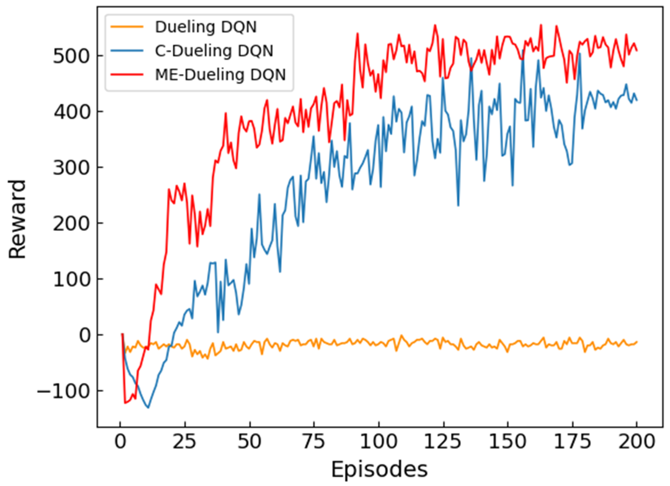
In order to verify the performance of the proposed algorithm, three algorithms including Dueling DQN (without any improvement), C-Dueling DQN (introducing a comprehensive reward function) and ME-Dueling DQN (introducing a comprehensive reward function and a memory-enhanced mechanism) are utilized for control experiments. The experiment is done in Scenario 1, where the initial position of the UH is $\left[0,50,1\right]$ and the position of the target radar is $\left[50,0,0\right]$. We have recorded the experimental process of 200 episodes, and the algorithm is updated 1000 times in each episode. Five independent experiments are performed for each algorithm, and the results of the five experiments are averaged as the final result.

Since the goal of deep reinforcement learning algorithms is to maximize the cumulative reward, the reward situation is an important indicator for evaluating the performance of the algorithm. Figure 5 records the cumulative situation of reward for each episode of the three algorithms. As shown in Figure 5, the performance of Dueling DQN is the worst among the three algorithms, and the entire training process is completed without convergence. This shows that the traditional reward setting cannot be based on algorithm feedback in time in the face of a large state space environment, and the sparse reward makes the algorithm difficult to converge. After training, both C-Dueling DQN and ME-Dueling DQN converge smoothly, which shows that the comprehensive reward function effectively improves the sparse reward problem and promotes algorithm convergence. The comparative analysis shows that the reward accumulation process of the ME-Dueling DQN algorithm is faster than that of the C-Dueling DQN algorithm, which shows that the memory-enhanced mechanism can effectively reduce the meaningless exploration in the early stage of training, making the algorithm faster to maximize the cumulative reward. Orientation update. It is worth noting that the cumulative reward of the two algorithms is not stable enough, because the existence of the $\epsilon -greedy$ strategy makes the algorithm have a certain probability to explore other non-optimal actions, which leads to the generation of oscillation.

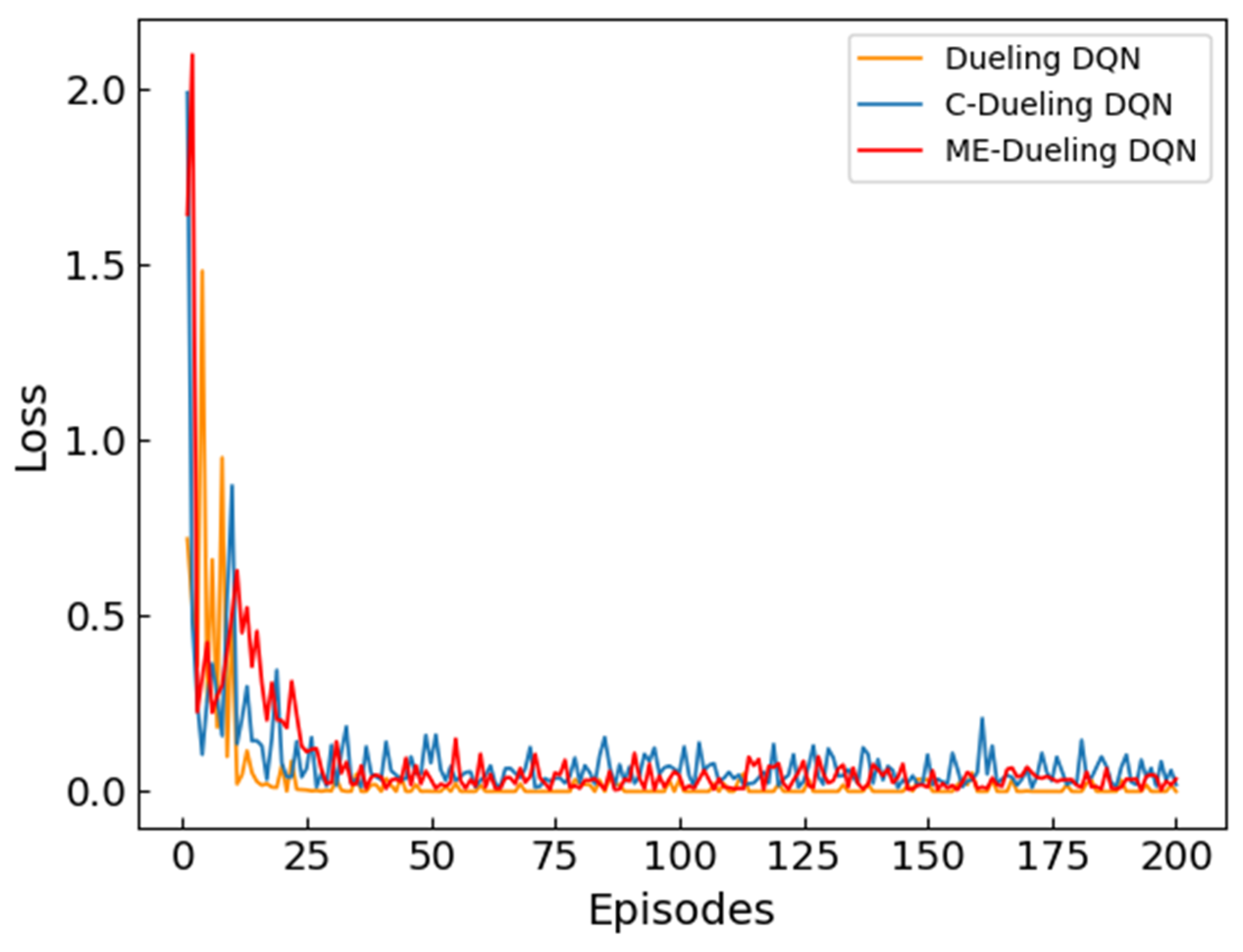
The loss value can reflect the update of the reinforcement learning algorithm and is another effective indicator to measure the performance of the algorithm. Figure 6 records the loss change during the training of the algorithm. As shown in Figure 6, the loss value of the Dueling DQN algorithm is 0 most of the time during the entire training process, indicating that it has not been effectively updated. The error values of the C-Dueling DQN and ME-Dueling DQN algorithms are at a large value in the initial stage of training, but they tend to be stable and maintain a small value after training. It shows that the comprehensive reward function can give feedback to the algorithm in time and prompt the algorithm to update quickly. Comparative analysis shows that in the initial stage of training, the loss value of the ME-Dueling DQN algorithm is larger than that of the C-Dueling DQN algorithm, indicating that the ME-Dueling DQN algorithm is updated faster in the early stage of training. This can indicate that the memory-enhanced mechanism can improve the learning ability of the algorithm in the early stage of training, because deep memory can promote learning more. In the later stage of training, the loss value of the ME-Dueling DQN algorithm is smaller and more stable than that of the C-Dueling DQN algorithm, indicating that the ME-Dueling DQN algorithm is more stable in the later stage of training. This shows that a memory-enhanced mechanism can improve the stability of the algorithm, because both good and bad memories are deepened, and meaningless exploration will be reduced.

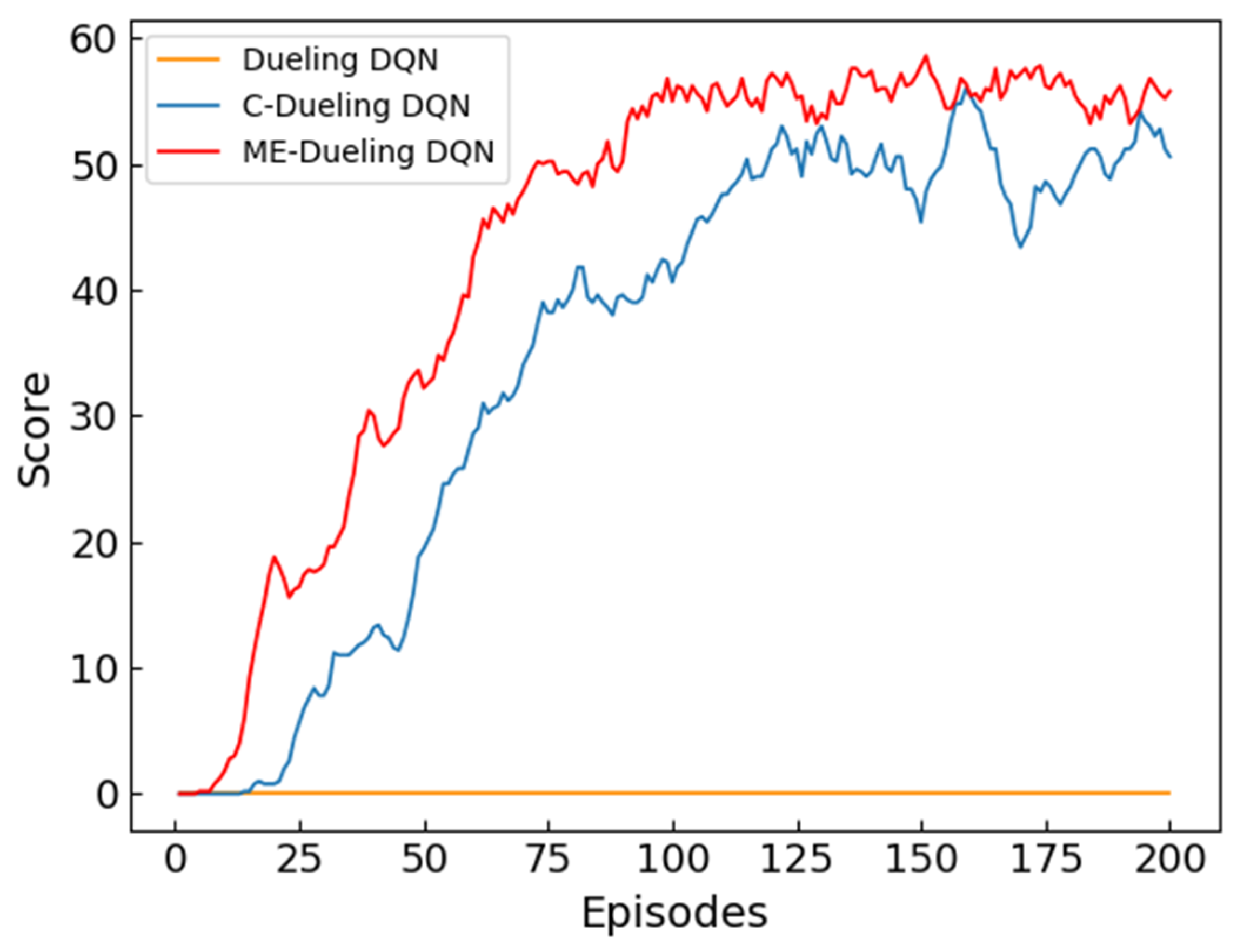
The score can be seen to be a good measure of the overall performance of the algorithm. The Figure 7 records the score of the three algorithms. As shown in Figure 7, the score of Dueling DQN is always 0 during the entire training process, indicating that it is difficult to complete the path planning task. After training, the score of C-Dueling DQN and ME-Dueling DQN eventually stabilizes within each episode. The comparative analysis shows that the overall score of the ME-Dueling DQN algorithm is higher than that of the C-Dueling DQN algorithm, indicating that the ME-Dueling DQN algorithm has a stronger ability to complete the path planning task. This shows that the memory-enhanced mechanism can effectively improve the algorithm’s ability to complete the task, because the memory of the crash and the memory of completing the task are repeatedly strengthened, which can promote the algorithm to avoid the threat area and complete the task as much as possible.

6.3. Influence of Straightness Coefficient

The purpose of introducing the straightness coefficient in the ME-Dueling DQN algorithm is to further optimize the planning path. Therefore, the effect of the straightness coefficient on the performance of the algorithm is a question worthy of discussion. We use the ME-Dueling DQN algorithm to analyze the effect of different values of the straightness coefficient on the performance of the algorithm and the planned path through multiple sets of control experiments. The experiment is done in Scenario 1, where the initial position of the UH is $\left[0,50,1\right]$ and the position of the target radar is $\left[50,0,0\right]$. We recorded the experimental process of 200 episodes, and the algorithm was updated 1000 times in each episode. Five independent experiments are performed for each set of parameters, and the results of the five experiments are averaged as the final result.

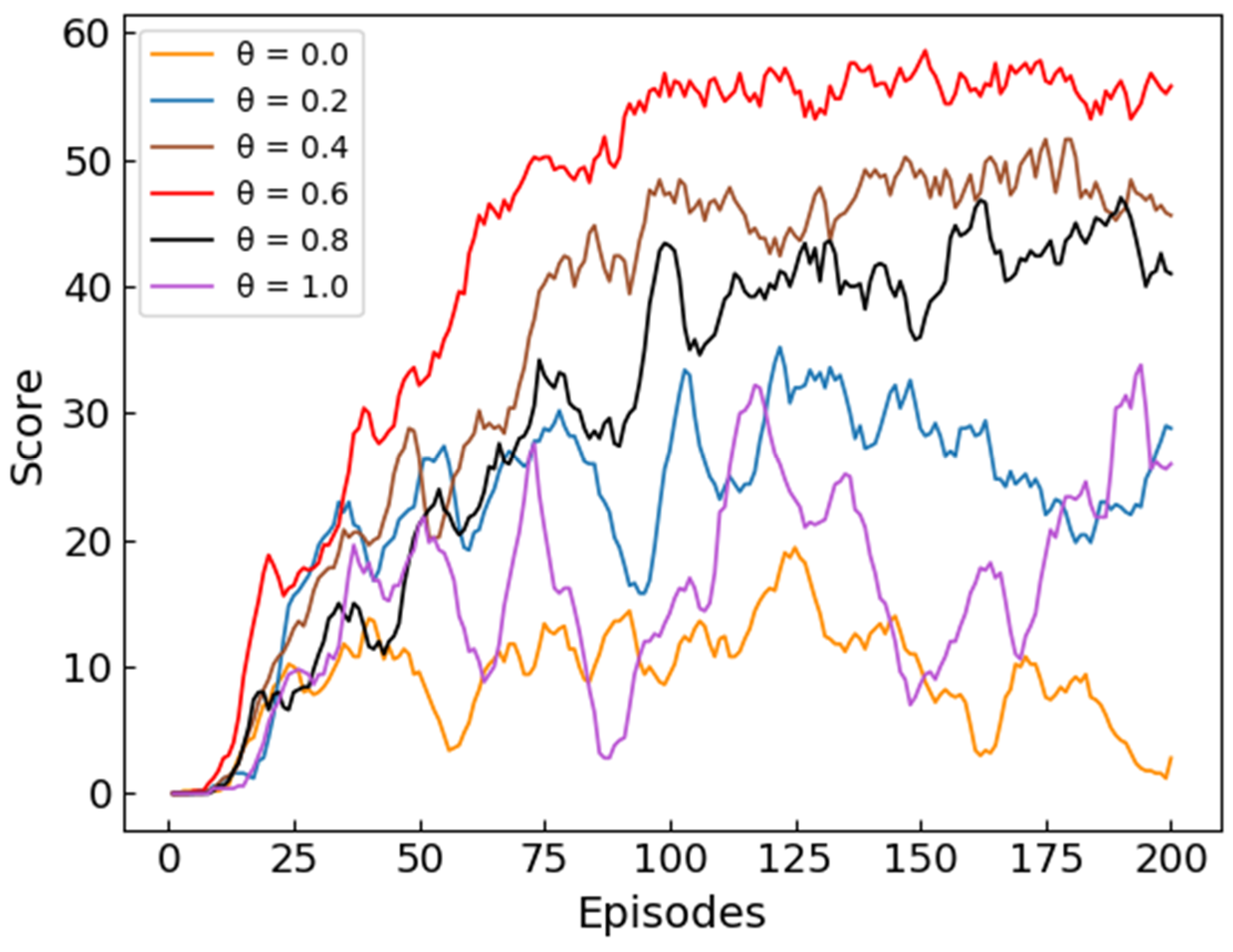
Figure 8 records the score of UH with different values of the straightness coefficient $\theta$. As shown in Figure 8, when the straightness coefficient $\theta$ takes different values, the convergence of the algorithm is different, and the final score is also different. This shows that the value of $\theta$ can not only affect the convergence of the algorithm, but also affect the ability of the algorithm to complete the path planning task. It can be seen from Figure 8 that when $\theta =0$, the performance of the algorithm is the worst in all cases, and the performance of the algorithm also improves as the value of $\theta$ increases. When $\theta =0.6$, the performance of the algorithm is the best in all cases, and the performance of the algorithm starts to deteriorate as the value of $\theta$ increases. The above situation can show that the introduction of the straightness coefficient $\theta$ effectively improves the performance of the algorithm. Since there are many dangerous areas in the environment, it may be easier to enter the dangerous area by frequently changing the flight direction. The introduction of the straightness coefficient $\theta$ can reduce the turning angle of the planned path, thereby reducing the possibility of UH encountering danger, thereby improving the performance of the algorithm. However, when the value of $\theta$ is greater than a certain value, its impact on the algorithm gradually becomes negative, because an overly straight path may not be able to avoid the danger ahead. Therefore, the performance of the algorithm can be effectively improved only when $\theta$ takes an appropriate value.

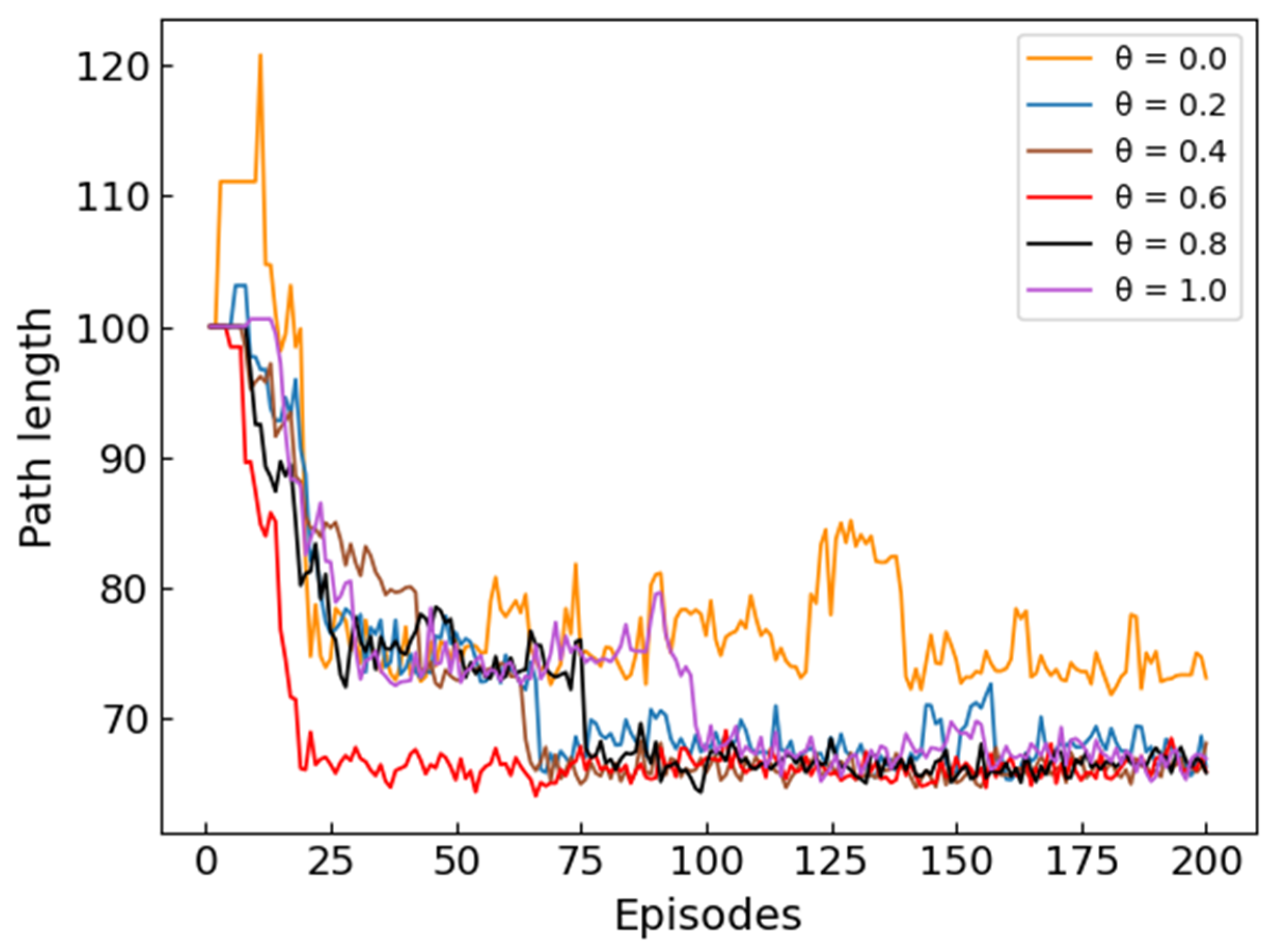
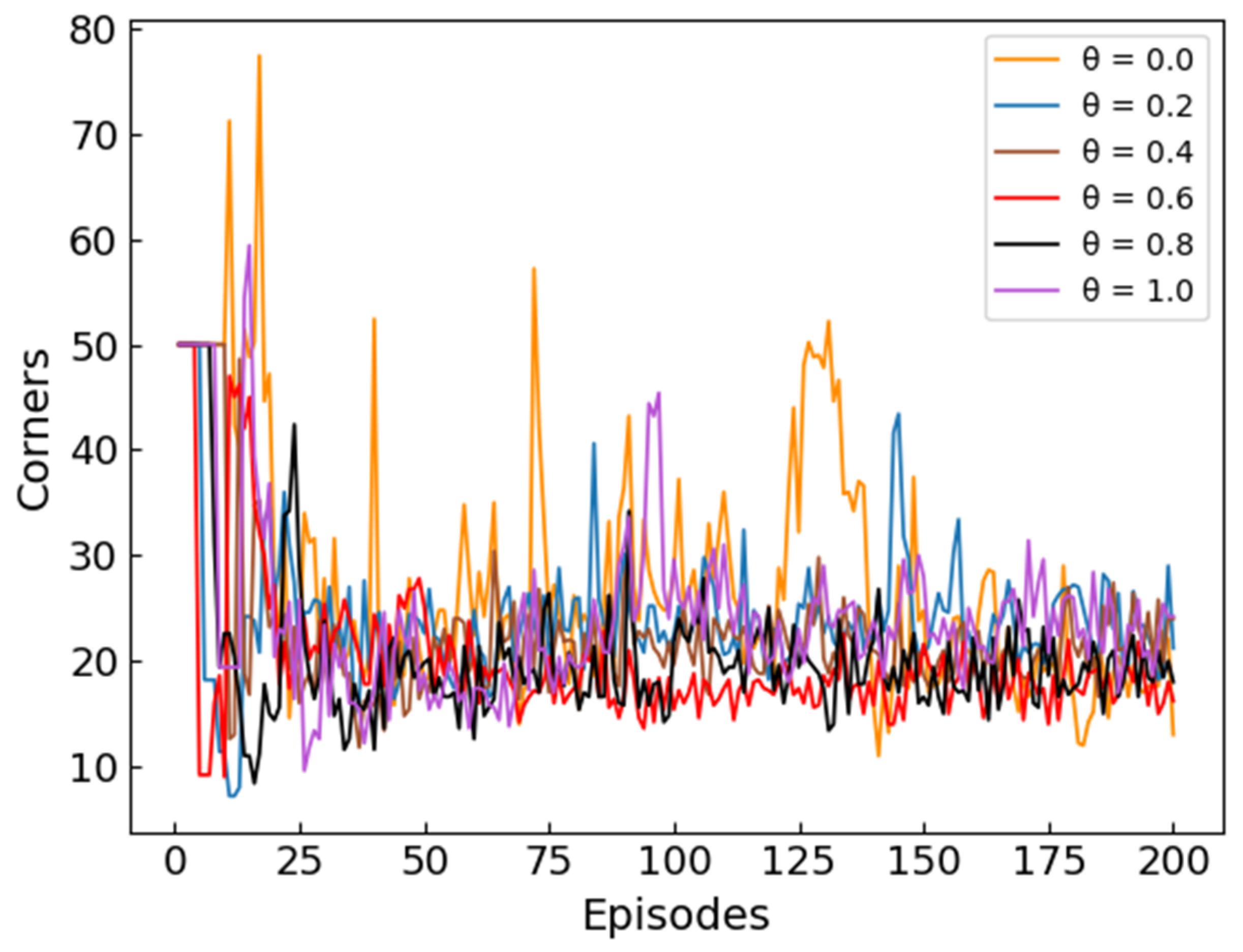
Figure 9 and Figure 10 respectively record the length of the planned path and the number of corners when the straightness coefficient $\theta$ takes different values. In order to make the changing trend of the curve clearer, the initial point of Figure 9 is set to 100, and the initial point of Figure 10 is set to 50. Combining Figure 9 and Figure 10, it can be seen that when $\theta =0$, the length of the planned path is the longest in all cases, and the number of corners is also the largest. As the value of $\theta$ increases, the length of the planned path decreases and the number of turns decreases. When $\theta$ is greater than a certain value, the length of the planned path begins to increase and the number of turns also increases. These situations can illustrate that the introduction of the straightness coefficient $\theta$ can reduce the length and number of corners of the planned path, thereby making the planned path straighter. It is worth noting that the path length and the number of corners is not completely positively correlated. Since the movement distances of UH in the horizontal and vertical directions are not exactly equal (0.5 km in the horizontal direction and 0.05 km in the vertical direction), a higher number of corners does not mean a longer path length. Combining the experimental results of Figure 8, Figure 9 and Figure 10, it can be seen that the ME-Dueling DQN algorithm can have the best performance when $\theta =0.6$.

6.4. Algorithm Suitability Test

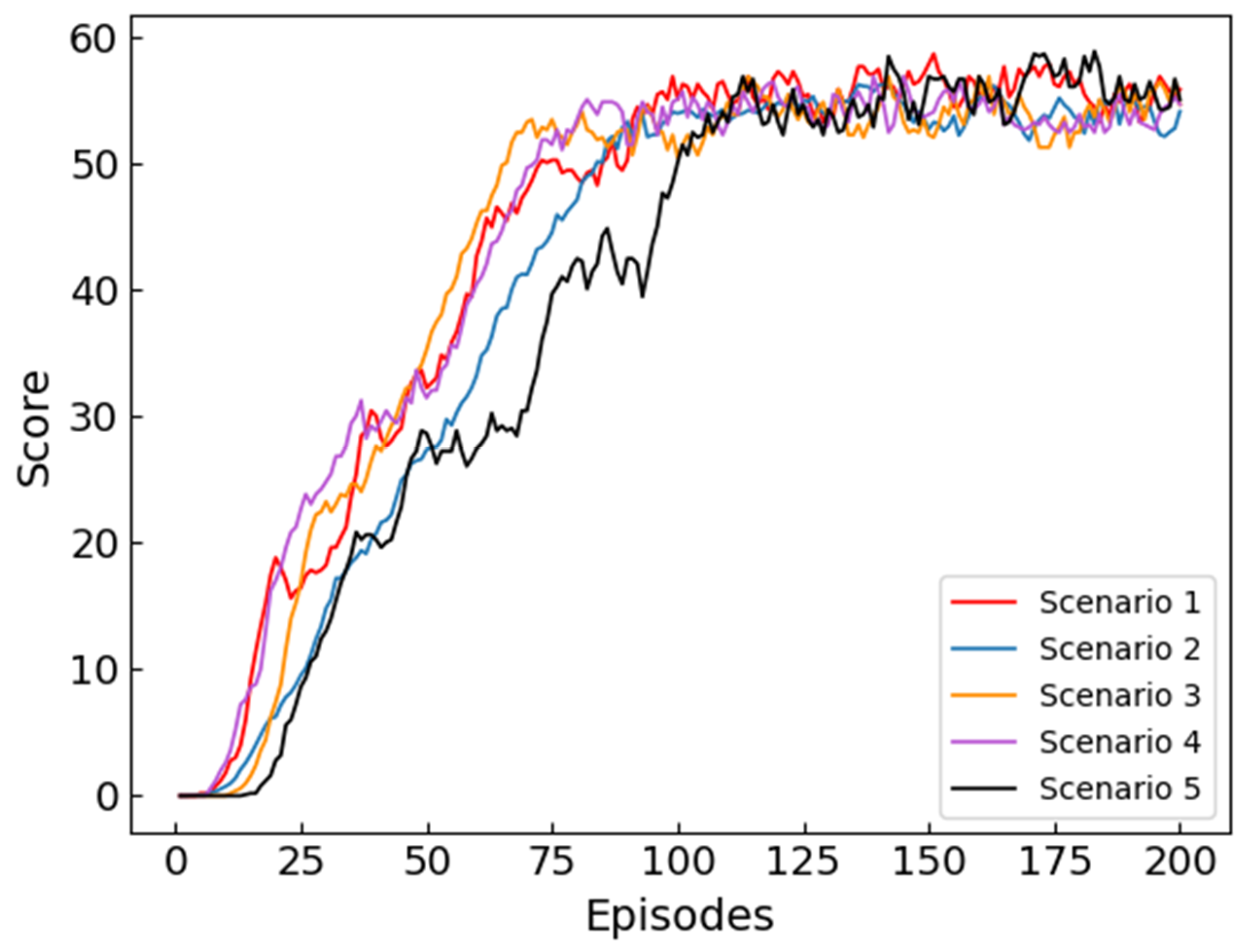
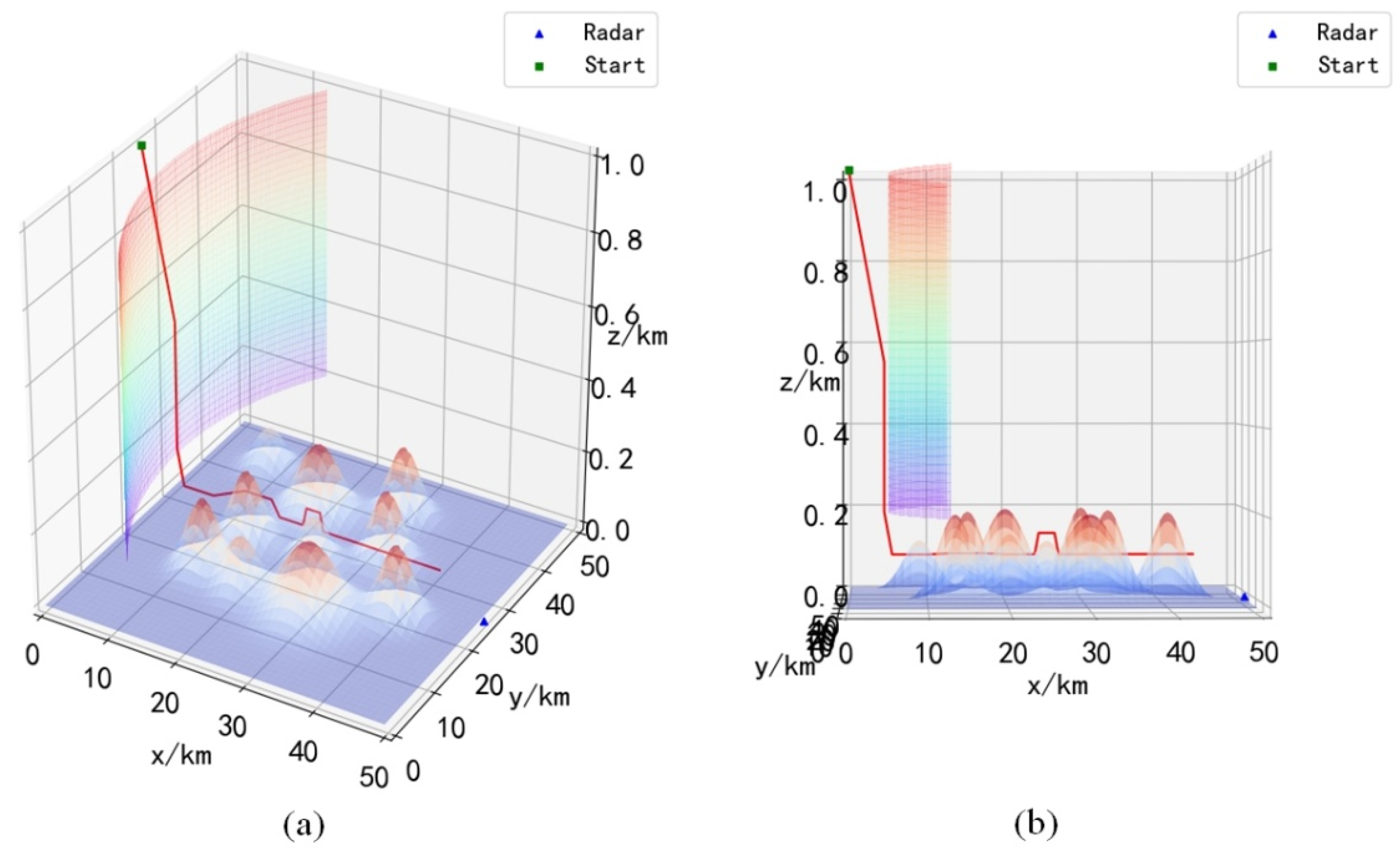
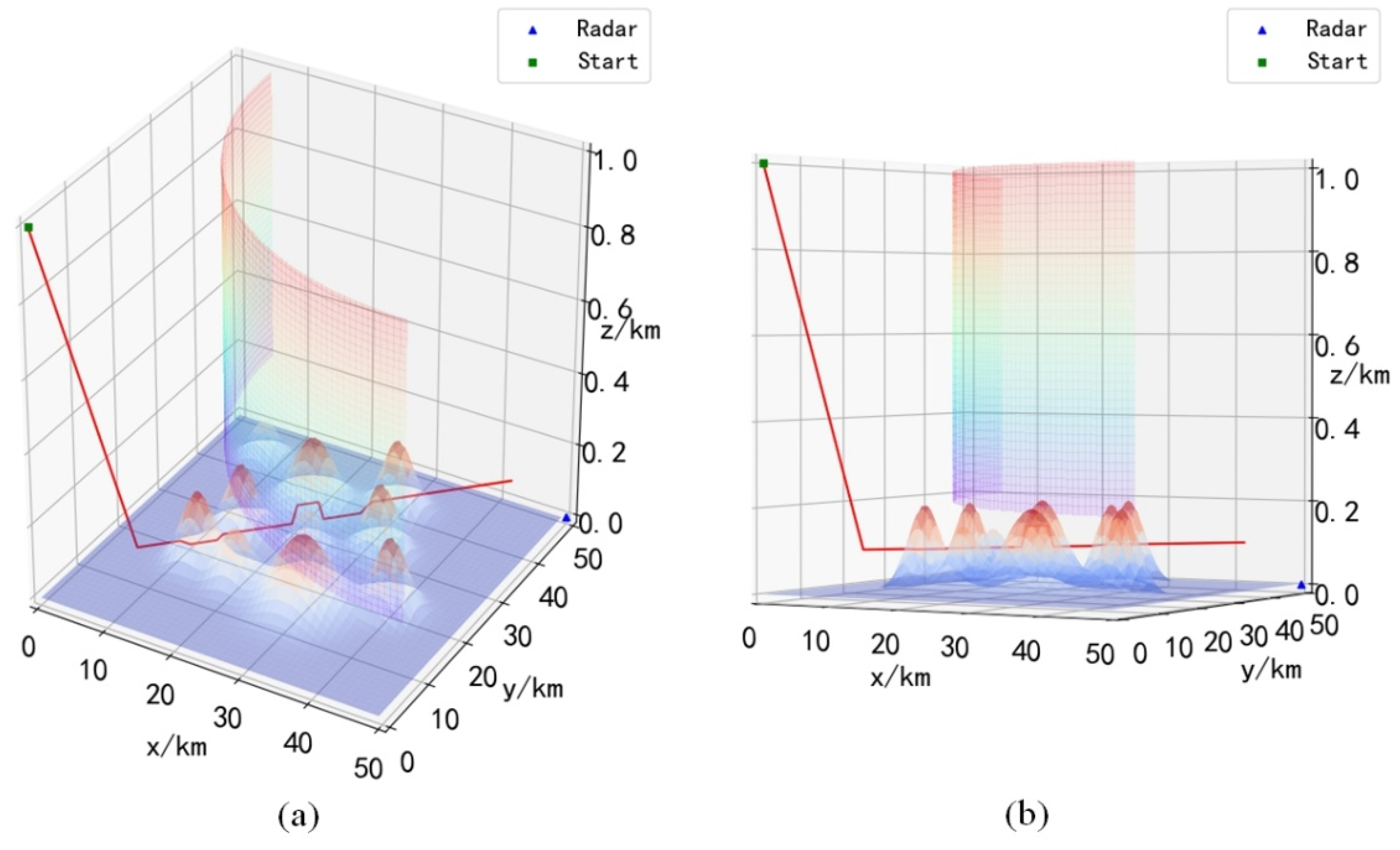
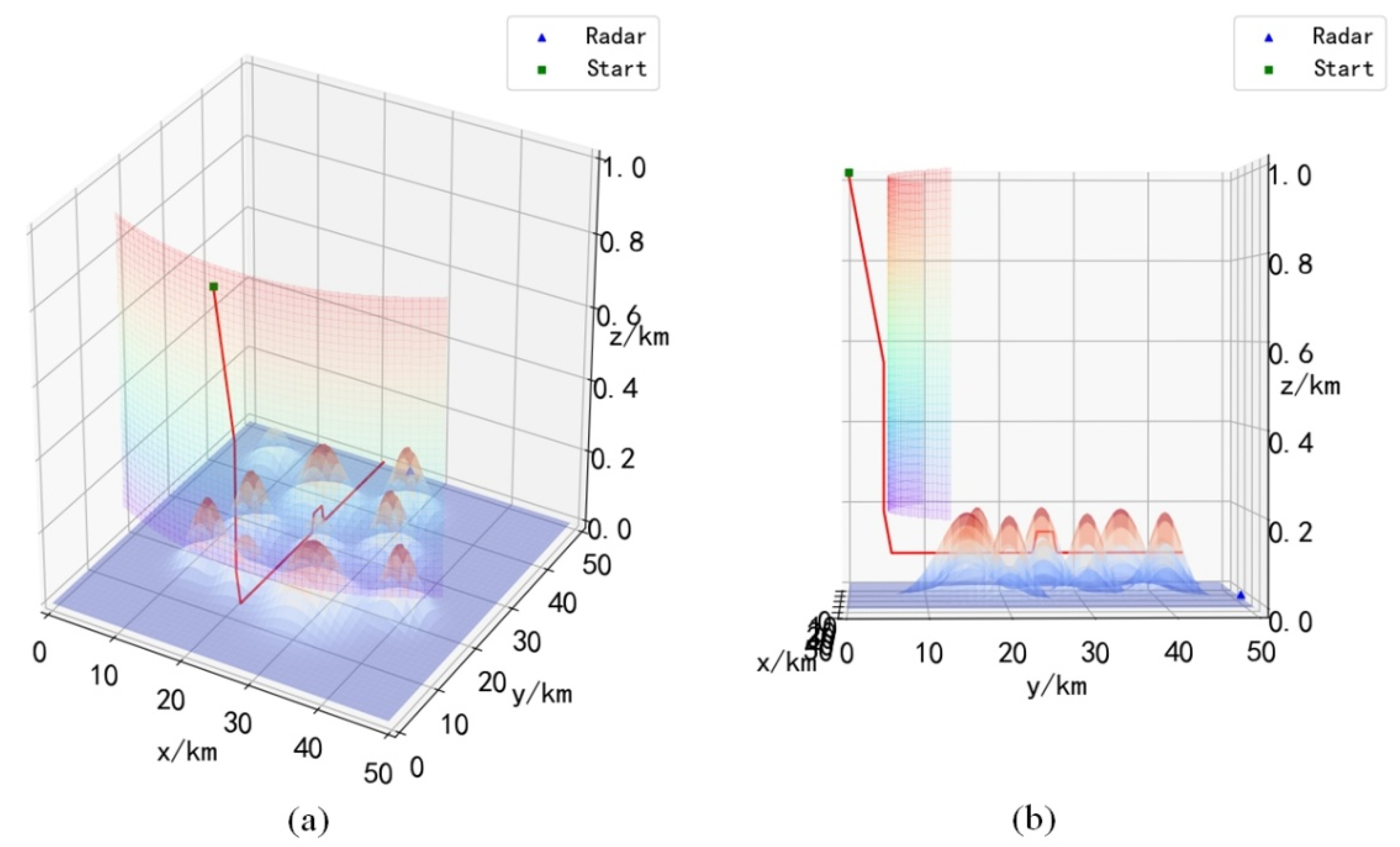
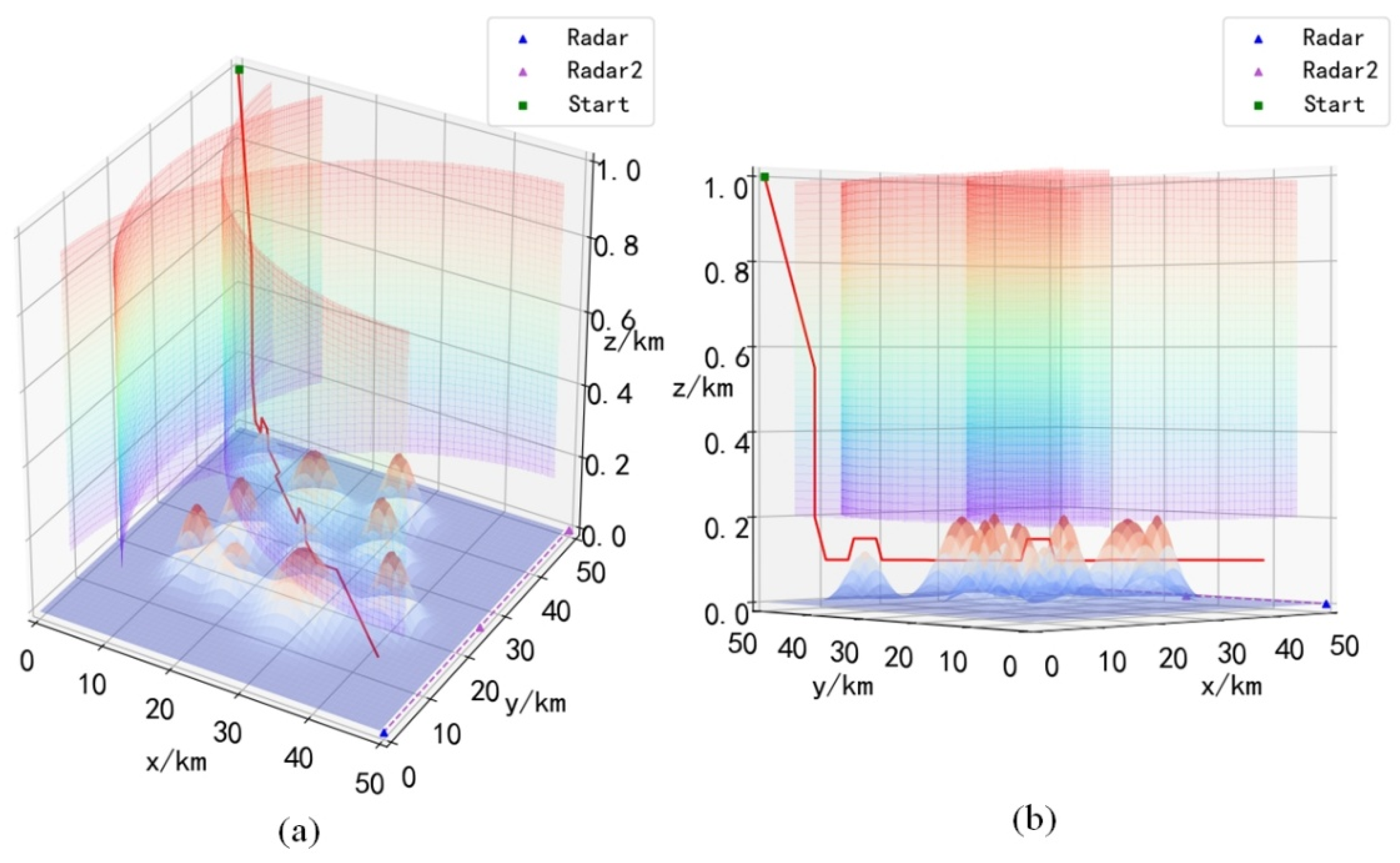
In order to verify the ability of the ME-Dueling DQN algorithm to adapt to various environments, we choose different environments for path planning tests. By changing the positions of the starting point and the target point, we construct four scenarios, Scenario 1: the initial position of the UH is $\left[0,50,1\right]$, and the position of the target radar is $\left[50,0,0\right]$. Scenario 2: The initial position of the UH is $\left[0,25,1\right]$ and the position of the target radar is $\left[50,25,0\right]$. Scenario 3: The initial position of the UH is $\left[0,0,1\right]$ and the position of the target radar is $\left[50,50,0\right]$. Scenario 4: The initial position of the UH is $\left[25,0,1\right]$ and the position of the target radar is $\left[25,50,0\right]$. In addition, we construct a dynamic scene with variable radar coverage by introducing a second on-board radar that can move. Scenario 5: The initial position of the UH is $\left[0,50,1\right]$, and the position of the target radar is $\left[50,0,0\right]$. The moving vehicle radar will start from $\left[50,50,0\right]$ and make a round-trip motion along the y-axis to $\left[50,0,0\right]$. Considering that the moving speed of the vehicle radar is much lower than that of the UH, it is set that the UH does two movements and the vehicle radar does one movement.

Figure 11 records the score of the path planning test using the ME-Dueling DQN algorithm in 5 scenarios. As shown in Figure 11, the ME-Dueling DQN algorithm can converge quickly in all five scenarios. Comparative analysis shows that the convergence speed of the ME-Dueling DQN algorithm in scenario 5 is slower and more oscillating than in the other four scenarios. Since there are moving radar vehicles in scenario 5, the radar coverage area is changing, and it takes more time to accurately identify the radar coverage area.

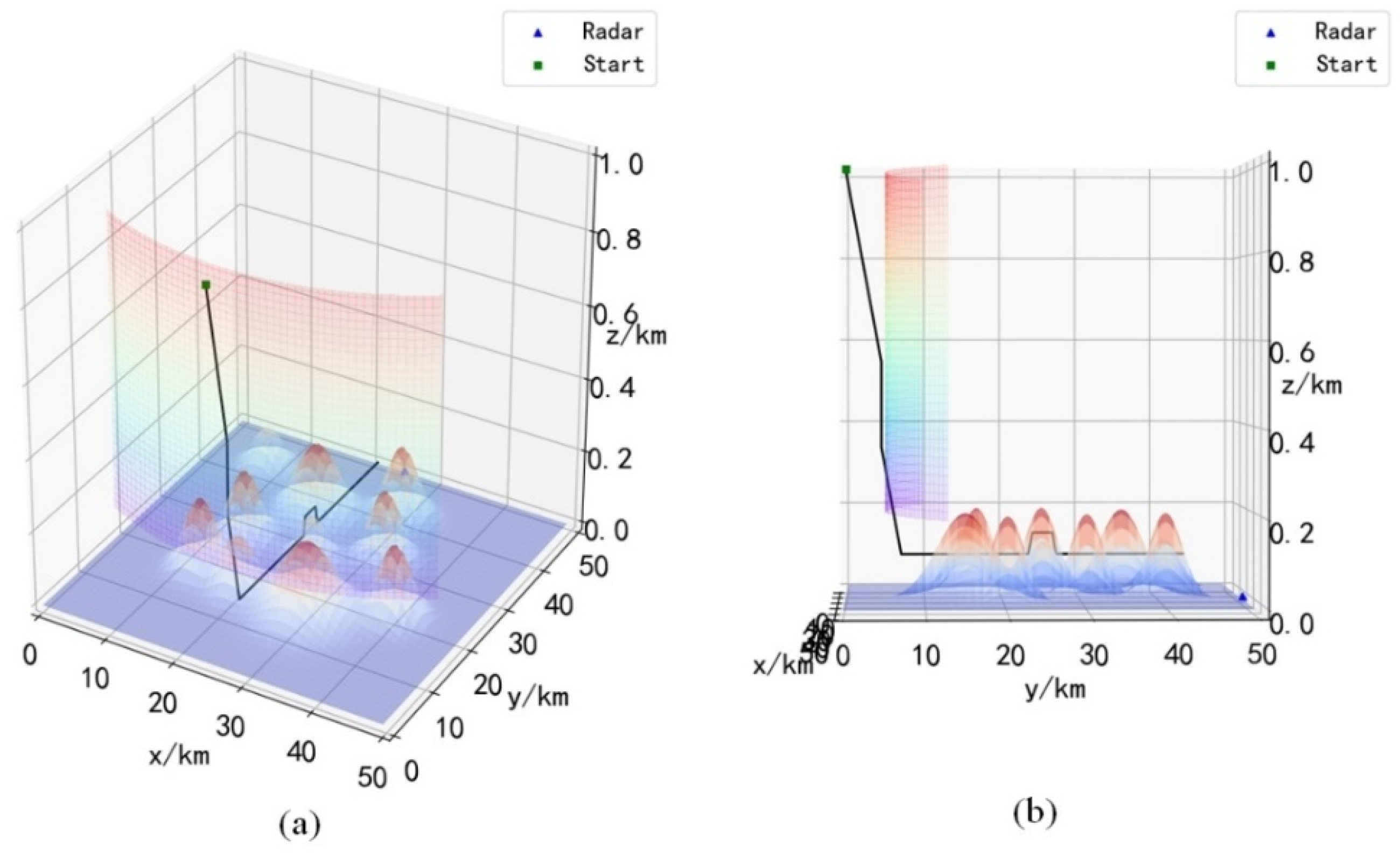
Combining Figure 12, Figure 13, Figure 14 and Figure 15, it can be seen that the UH after training will choose the descending height before entering the radar coverage area, and reach the strike area by flying at a low altitude, and the UH will choose the optimal action to avoid the mountains ahead during the flight. It is worth noting that during obstacle avoidance, the UH can fly over the obstacle, or go around the obstacle, which can be verified in Figure 12a, Figure 13a and Figure 14a. This shows that the trained UH will autonomously choose the optimal path when avoiding obstacles. Since the rewards obtained when choosing different paths to avoid obstacles are different, only choosing the optimal path will maximize the cumulative reward.

In the process of the algorithm interacting with the environment, once the UH crashes (the UH hits the mountain or is detected by the radar), the current path will be considered unsafe, and the algorithm will receive a negative reward. Although detection by radar within the radar area is probabilistically distributed, the complete radar coverage area can also be explored after the algorithm has fully interacted with the environment. Since the purpose of the ME-Dueling DQN algorithm learning is to maximize the cumulative reward, after the algorithm converges, it will choose the optimal flight path to avoid crashes as much as possible. It can be seen from Figure 16 that although the position of the mobile radar vehicle is changing, the ME-Dueling DQN algorithm still explores the optimal path. In Figure 16, UH chooses to descend the flight height at the fastest speed, perfectly avoiding radar detection at all positions, indicating that it has accurately detected all potentially dangerous areas. To sum up, the ME-Dueling DQN algorithm has good environmental adaptability and can help UH successfully complete the raid mission.

6.5. Compared with Traditional Algorithms

In order to further verify the good performance of the ME-Dueling DQN algorithm, we select the Dijkstra and A* algorithms for control experiments. During the experiment, the $u\left(k\right)$ calculation of the A* algorithm uses the Manhattan distance. The Dijkstra and A* algorithms are used to conduct a large number of path planning tests in scenarios 1 to 5, respectively. The test results show that the Dijkstra and A* algorithms can successfully plan safe paths in scenarios 1 to 5, and in some cases these paths are the same as the path planned by the ME-Dueling DQN algorithm is consistent. 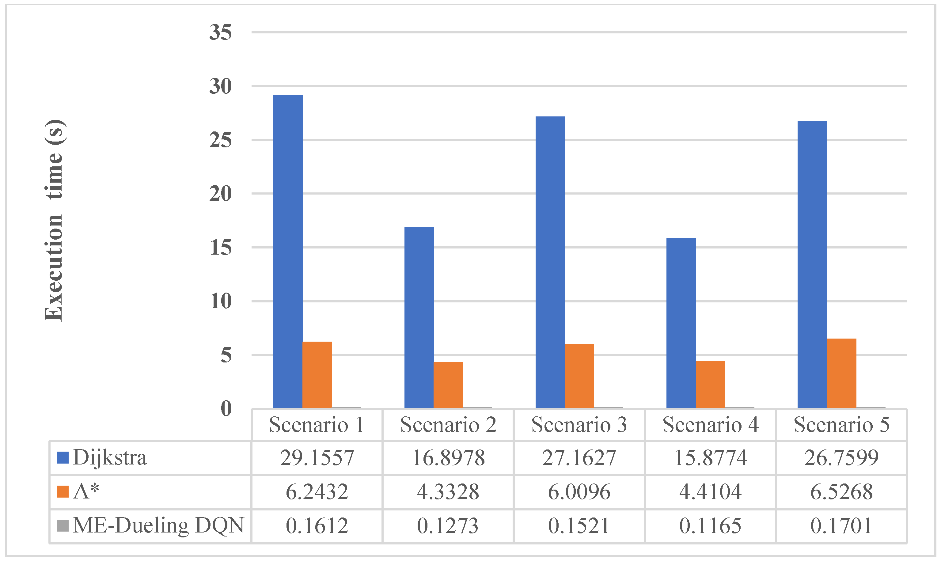However, the test results show that the safe paths planned by the Dijkstra and A* algorithms may cross the radar coverage area in some cases, as shown in Figure 17. In addition, we recorded the execution time of the Dijkstra, A* and ME-Dueling DQN algorithms in the path planning test under various scenarios, as shown in Figure 18. The execution time in the figures is obtained by averaging the results of five independent experiments.

Figure 17 is a special case we selected from multiple test results. Since the paths planned by the Dijkstra and A* algorithms are consistent in most cases, Figure 17 can represent the test results of the two algorithms at the same time. It can be seen from Figure 17 that the UH entered the radar coverage area during the process of descending the flight altitude in the early stage of the mission. The analysis shows that the radar cannot accurately detect the target within the height of 0.2–0.4 km, that is, this area is not completely covered by the radar. The Dijkstra and A* algorithms will consider the uncovered areas to be safe during the path search process, so they will pass through these areas. However, the radar coverage area is probabilistically distributed, and the location of the covered area will change. Therefore, absolute safety can only be guaranteed if the radar detection range is completely avoided. To sum up, the Dijkstra and A* algorithms cannot plan a safe and reliable flight path for UH in this complex battlefield environment.

It can be seen from Section 6.4 that the path planned by Algorithm ME-Dueling DQN has not crossed the radar detection area. This is because, under the action of the reward mechanism, the ME-Dueling DQN algorithm will remember the position detected by the radar during the path search process. When the ME-Dueling DQN algorithm fully interacts with the environment, the radar detection range will be regarded as a restricted area and will no longer be entered. Therefore, the path planned by the ME-Dueling DQN algorithm can completely avoid the radar detection area, which can ensure that the UH will not be detected by the radar.

As can be seen from Figure 18, in the test of each scenario, the execution time of the Dijkstra algorithm is the longest, and the execution time of the A* algorithm is much shorter than that of the Dijkstra algorithm. The ME-Dueling DQN algorithm has the shortest execution time among the three algorithms, and is much shorter than the other two algorithms. Analysis shows that the Dijkstra algorithm needs to calculate the shortest path length from the starting point to all other points in the iterative process, which is a divergent search algorithm. The A* algorithm is a heuristic search algorithm, which also calculates the expected cost from the current point to the endpoint. During the execution of the algorithm, the search space of the A* algorithm is much smaller than that of the Dijkstra algorithm, and so the execution time of its path search is smaller than that of the Dijkstra algorithm. In the process of path planning test, the ME-Dueling DQN algorithm only needs to judge the correct action corresponding to the current state through the neural network, and does not need to search for the path, so its path planning speed is naturally much faster than that of the Dijkstra and A* algorithms. It is worth noting that for the ME-Dueling DQN algorithm, the execution time of our comparison is performed using the already trained neural network, and the network training time is not calculated.

7. Conclusions

In order to solve the UH perform raid missions in the low airspace path planning problem in a 3D complex dynamic environment, a memory-enhanced dueling deep Q-network algorithm was proposed in this paper. A 3D environment model was built for UH to perform low-altitude raid missions, and the state set and action set are divided. On this basis, a comprehensive reward function is designed, which can guide the proposed algorithm to converge quickly and optimize the planning path. In order to further speed up the algorithm convergence and reduce meaningless exploration, a memory-enhanced mechanism is proposed. The effects of a comprehensive reward function and memory-enhanced mechanism on the performance of the algorithm were compared and analyzed through simulation experiments. The experimental results showed that the comprehensive reward function and the memory enhancement mechanism can effectively promote the convergence of the algorithm and improve the overall performance of the algorithm. In addition, the path planning ability of the proposed algorithm was verified in different scenarios, and the results showed that the proposed algorithm can plan a safe and reliable flight path for UH in complex dynamic environments. In future works, we will consider the introduction of the memory-enhanced mechanism into more intelligent algorithms to verify its generality.

References

1. Space, H.H. Helicopter. In Flight and Motion; Routledge: New York, NY, USA, 2015; pp. 280–287. [Google Scholar]
2. De Durand, E.; Michel, B.; Tenenbaum, E. Helicopter Warfare. Focus Stratégique. 2012, 32, 9–17. [Google Scholar]
3. Yuan, J.; Zhang, X.; Wang, S. The effect of helicopter low altitude cruise on the efficiency of radar detection. In Proceedings of the 2017 2nd International Conference on Mechatronics and Information Technology (ICMIT 2017), Xi’an, China, 26–27 August 2017. [Google Scholar]
4. Zhao, Y.; Zheng, Z.; Liu, Y. Survey on Computational-Intelligence-Based UAV Path Planning. Knowl.-Based Syst. 2018, 158, 54–64. [Google Scholar] [CrossRef]
5. Roberge, V.; Tarbouchi, M.; Labonté, G. Comparison of parallel genetic algorithm and particle swarm optimization for real-time UAV path planning. IEEE Trans. Ind. Inform. 2012, 9, 132–141. [Google Scholar] [CrossRef]
6. Pandey, P.; Shukla, A.; Tiwari, R. Three-dimensional path planning for unmanned aerial vehicles using glowworm swarm optimization algorithm. Int. J. Syst. Assur. Eng. Manag. 2018, 9, 836–852. [Google Scholar] [CrossRef]
7. Dewangan, R.K.; Shukla, A.; Godfrey, W.W. Three dimensional path planning using grey wolf optimizer for UAVs. Appl. Intell. 2019, 49, 2201–2217. [Google Scholar] [CrossRef]
8. Zhou, X.; Gao, F.; Fang, X.; Lan, Z. Improved bat algorithm for UAV path planning in three-dimensional space. IEEE Access 2021, 9, 20100–20116. [Google Scholar] [CrossRef]
9. Luo, M.; Hou, X.; Yang, J. Surface optimal path planning using an extended Dijkstra algorithm. IEEE Access 2020, 8, 147827–147838. [Google Scholar] [CrossRef]
10. Wang, N.; Jin, X.; Er, M.J. A multilayer path planner for a USV under complex marine environments. Ocean Eng. 2019, 184, 1–10. [Google Scholar] [CrossRef]
11. Yao, J.; Li, X.; Zhang, Y.; Liu, Y. Path Planning of Unmanned Helicopter in Complex Dynamic Environment Based on State-Coded Deep Q-Network. Symmetry 2022, 14, 856. [Google Scholar] [CrossRef]
12. Singh, Y.; Sharma, S.; Sutton, R.; Hatton, D.; Khan, A. A constrained A* approach towards optimal path planning for an unmanned surface vehicle in a maritime environment containing dynamic obstacles and ocean currents. Ocean Eng. 2018, 169, 187–201. [Google Scholar] [CrossRef]
13. Mnih, V.; Kavukcuoglu, K.; Silver, D.; Rusu, A.A.; Veness, J.; Bellemare, M.G.; Graves, A.; Riedmiller, M.; Fidjeland, A.K.; Ostrovski, G. Human-level control through deep reinforcement learning. Nature 2015, 518, 529–533. [Google Scholar] [CrossRef]
14. Li, Y. Deep reinforcement learning: An Overview. arXiv 2017, arXiv:1701.07274. [Google Scholar]
15. Majeed, A.; Hwang, S.O. A multi-objective coverage path planning algorithm for UAVs to cover spatially distributed regions in urban environments. Aerospace 2021, 8, 343. [Google Scholar] [CrossRef]
16. Soltani, A.R.; Tawfik, H.; Goulermas, J.Y.; Fernando, T. Path planning in construction sites: Performance Evaluation of the Dijkstra, A*, and GA search algorithms. Adv. Eng. Inform. 2002, 16, 291–303. [Google Scholar] [CrossRef]
17. Guo, S.; Zhang, X.; Du, Y.; Zheng, Y.; Cao, Z. Path planning of coastal ships based on optimized DQN reward function. J. Mar. Sci. Eng. 2021, 9, 210. [Google Scholar] [CrossRef]
18. Zafar, M.N.; Mohanta, J.C. Methodology for path planning and optimization of mobile robots: A Review. Proced. Comput. Sci. 2018, 133, 141–152. [Google Scholar] [CrossRef]
19. Henkel, C.; Bubeck, A.; Xu, W. Energy efficient dynamic window approach for local path planning in mobile service robotics. IFAC-PapersOnLine 2016, 49, 32–37. [Google Scholar] [CrossRef]
20. Yao, W.R.; Qi, N.M.; Liu, Y.F. Online Trajectory Generation with Rendezvous for UAVs Using Multistage Path Prediction. J. Aerosp. Eng. 2017, 30, 04016092.1–04016092.10. [Google Scholar] [CrossRef]
21. Zeng, Z.; Sammut, K.; Lammas, A.; He, F.; Tang, Y. Efficient Path Re-planning for AUVs Operating in Spatiotemporal Currents. J. Intell. Robot. Syst. 2015, 79, 135–153. [Google Scholar] [CrossRef]
22. Duan, H.; Yu, Y.; Zhang, X.; Shao, S. Three-dimension path planning for UCAV using hybrid meta-heuristic ACO-DE algorithm. Simul. Model. Pract. Theory 2010, 18, 1104–1115. [Google Scholar] [CrossRef]
23. Shorakaei, H.; Vahdani, M.; Imani, B.; Gholami, A. Optimal cooperative path planning of unmanned aerial vehicles by a parallel genetic algorithm. Robot 2016, 34, 823–836. [Google Scholar] [CrossRef]
24. Shangguan, L.; Thomasson, J.A.; Gopalswamy, S. Motion Planning for Autonomous Grain Carts. IEEE Trans. Veh. Technol. 2021, 70, 2112–2123. [Google Scholar] [CrossRef]
25. Hu, R.; Zhang, Y. Fast Path Planning for Long-Range Planetary Roving Based on a Hierarchical Framework and Deep Reinforcement Learning. Aerospace 2022, 9, 101. [Google Scholar] [CrossRef]
26. Chen, C.; Chen, X.Q.; Ma, F.; Zeng, X.J.; Wang, J. A knowledge-free path planning approach for smart ships based on reinforcement learning. Ocean Eng. 2019, 189, 106–299. [Google Scholar] [CrossRef]
27. Benhlima, S.; Lamini, C.; Fathi, Y. H-MAS architecture and reinforcement learning method for autonomous robot path planning. In Proceedings of the 2017 Intelligent Systems and Computer Vision (ISCV), Fez, Morocco, 17–19 April 2017; pp. 1–7. [Google Scholar]
28. Maoudj, A.; Hentout, A. Optimal path planning approach based on Q-learning algorithm for mobile robots. Appl. Soft Comput 2020, 97, 106796. [Google Scholar] [CrossRef]
29. Fan, J.; Wang, Z.; Xie, Y.; Yang, Z. A theoretical analysis of deep Q-learning. In Proceedings of the Learning for Dynamics and Control, PMLR, Berkeley, USA, 11–12 June 2020; pp. 486–489. [Google Scholar]
30. Lv, L.; Zhang, S.; Ding, D.; Wang, Y. Path Planning via an Improved DQN-based Learning Policy. IEEE Access 2019, 7, 67319–67330. [Google Scholar] [CrossRef]
31. Zhu, Z.; Hu, C.; Zhu, C.; Zhu, Y.; Sheng, Y. An Improved Dueling Deep Double-Q Network Based on Prioritized Experience Replay for Path Planning of Unmanned Surface Vehicles. J. Mar. Sci. Eng. 2021, 9, 1267. [Google Scholar] [CrossRef]
32. Wen, S.; Lv, X.; Lam, H.K.; Fan, S.; Yuan, X.; Chen, M. Probability Dueling DQN active visual SLAM for autonomous navigation in indoor environment. Ind. Robot 2021. ahead-of-print. [Google Scholar] [CrossRef]
33. Wu, X.; Chen, H.; Chen, C.; Zhong, M.; Xie, S.; Guo, Y.; Fujita, H. The autonomous navigation and obstacle avoidance for USVs with ANOA deep reinforcement learning method. Knowl.-Based Syst. 2020, 196, 105201. [Google Scholar] [CrossRef]
34. Wang, Z.; Schaul, T.; Hessel, M.; Hasselt, H.; Lanctot, M.; Freitas, N. Dueling network architectures for deep reinforcement learning. In Proceedings of the International Conference on Machine Learning, JMLR, New York, NY, USA, 19–24 June 2016; pp. 1995–2003. [Google Scholar]
35. Wang, H.; Yu, Y.; Yuan, Q. Application of Dijkstra algorithm in robot path-planning. In Proceedings of the 2011 Second International Conference on Mechanic Automation and Control Engineering, Inner Mongolia, China, 18 August 2011; pp. 1067–1069. [Google Scholar]
36. Ferguson, D.; Stentz, A. Using interpolation to improve path planning: The Field D* algorithm. J. Fld. Robot. 2006, 23, 79–101. [Google Scholar] [CrossRef]
37. Wiering, M.A.; Van Otterlo, M. Reinforcement learning. Adapt. Learn. Optim. 2012, 12, 729. [Google Scholar]
38. Melo, F.S. Convergence of Q-Learning: A Simple Proof; Technology Represent; Institute of Systems and Robotics: Lisboa, Portugal, 2001; pp. 1–4. [Google Scholar]
39. Zhang, S.; Sutton, R.S. A deeper look at experience replay. arXiv 2017, arXiv:1712.01275. [Google Scholar]
40. Sewak, M. Deep q network (dqn), double dqn, and dueling dqn. In Deep Reinforcement Learning; Springer: Singapore, 2019; pp. 95–108. [Google Scholar]
41. Han, G.L. Automatic Parking Path Planning Based on Ant Colony Optimization and the Grid Method. J. Sens. 2021, 2021, 8592558. [Google Scholar] [CrossRef]
42. Memarian, F.; Goo, W.; Lioutikov, R.; Niekum, S.; Topcu, U. Self-supervised online reward shaping in sparse-reward environments. In Proceedings of the 2021 IEEE/RSJ International Conference on Intelligent Robots and Systems (IROS), Prague, Czech, 16 December 2021; pp. 2369–2375. [Google Scholar]
43. Zhang, H.; Qu, C.; Zhang, J.; Li, J. Self-Adaptive Priority Correction for Prioritized Experience Replay. Appl. Sci. 2020, 10, 6925. [Google Scholar] [CrossRef]
Figure 1. Battlefield environment. The colored curved surface is the radar detection boundary.
Aerospace 09 00417 g001
Figure 2. Movement of unmanned helicopters.
Aerospace 09 00417 g002
Figure 3. Probability of unmanned helicopter being detected by radar.
Aerospace 09 00417 g003
Figure 4. Memory-enhanced dueling deep q-network model.
Aerospace 09 00417 g004
Figure 5. The convergence analysis of each algorithm.
Aerospace 09 00417 g005
Figure 6. The loss change process of each algorithm.
Aerospace 09 00417 g006
Figure 7. The score change process of each algorithm.
Aerospace 09 00417 g007
Figure 8. The reward accumulation process of each set of parameters.
Aerospace 09 00417 g008
Figure 9. The path length change process of each set of parameters.
Aerospace 09 00417 g009
Figure 10. The corners change process of each set of parameters.
Aerospace 09 00417 g010
Figure 11. The score change process of path planning in five scenarios.
Aerospace 09 00417 g011
Figure 12. The path planning result in scenario 1. (a) is the full view of the path, (b) is the side view of the path.
Aerospace 09 00417 g012
Figure 13. The path planning result in scenario 2. (a) is the full view of the path, (b) is the side view of the path.
Aerospace 09 00417 g013
Figure 14. The path planning result in scenario 3. (a) is the full view of the path, (b) is the side view of the path.
Aerospace 09 00417 g014
Figure 15. The path planning result in scenario 4. (a) is the full view of the path, (b) is the side view of the path.
Aerospace 09 00417 g015
Figure 16. The path planning result in scenario 5. (a) is the full view of the path, (b) is the side view of the path. The purple dotted line is the trajectory of the vehicle radar, and we have drawn its radar detection boundary at three special positions 50 , 50 , 0 , 50 , 25 , 0 and 50 , 0 , 0 .
Aerospace 09 00417 g016
Figure 17. The path planning result by Dijkstra and A* algorithms in scenario 4. (a) is the full view of the path, (b) is the side view of the path.
Aerospace 09 00417 g017
Figure 18. Comparison of execution time for Dijkstra, A* and ME-Dueling DQN algorithms.
Aerospace 09 00417 g018