Spectral Light Curve Simulation for Parameter Estimation from Space Debris

Abstract

Characterisation of space debris has become a fundamental task to facilitate sustainable space operations. Ground-based surveillance provides the means to extract key attributes from spacecraft. However, signal inversion attempts are generally under-constrained, which is why an increase in measurement channels through multispectral observations is expected to benefit parameter estimation. The current approach to simulating space debris observation at the Institute of Technical Physics of the German Aerospace Centre (DLR) in Stuttgart relies on monochromatic images taken from the POV-Ray render engine to form light curve signals. Rendered scenes are generated based on the location of an observer by propagating a target’s orbit and rotation. This paper describes the simulation of spectral light curves through the extension of DLR’s Raxus Prime simulation environment. Light reflections are computed using the Mitsuba2 spectral render engine, while atmospheric attenuation is accounted for by the radiative transfer library libRadTran. A validation of the simulator was achieved using multispectral measurements, carried out at the Uhlandshöhe research observatory in Stuttgart. Measured and synthetic data were found to be in agreement based on an RMS error <1% of the total measured signal count. Further, simulated spectral products were used to determine a target’s surface material composition and rotation state and examine aspects of laser ranging to non-cooperative targets.

1. Introduction

The congestion of Earth’s orbits has established itself as a growing threat to space operations today. Over the past years, the number of objects in orbit has surged, bringing with it an increased risk for fragmentation events through explosions or collisions [1]. Thereby, objects launched to lower earth orbit (LEO) alone have risen by more than 17 fold since 2012 [1]. Simulations based on extrapolations of the current launch traffic behaviour and successful de-orbiting measures have anticipated that, should explosion rates remain constant, the amount of objects in orbit is set to grow exponentially [1].

To counteract this trend, it will be essential to rethink sustainability in space. A key aspect of this is facilitating timely collision avoidance manoeuvres that rely on precise orbit predictions to minimise any impact damage. Current propagations largely stem from simple estimates of atmospheric drag and solar radiation pressure acting on targets, which are assumed to remain constant along the targets’ trajectories. This approach has come to be known as the cannonball model, as it neglects any variation caused by the objects’ orientation, shape and surface composition. However, the model has been shown to be inadequate, especially for objects with high area-to-mass ratios, for which a study by McMahon et al. found position errors greater than 1 $\mathrm{k}$$\mathrm{m}$ within a propagation time span of one hour [2]. Hence, including attitude and surface properties of targets into propagations can help combat limitations of the cannonball model and lead to more accurate orbit predictions [2]. Moreover, this information will also be crucial in enabling missions for in-orbit servicing and de-orbiting of space debris [3].

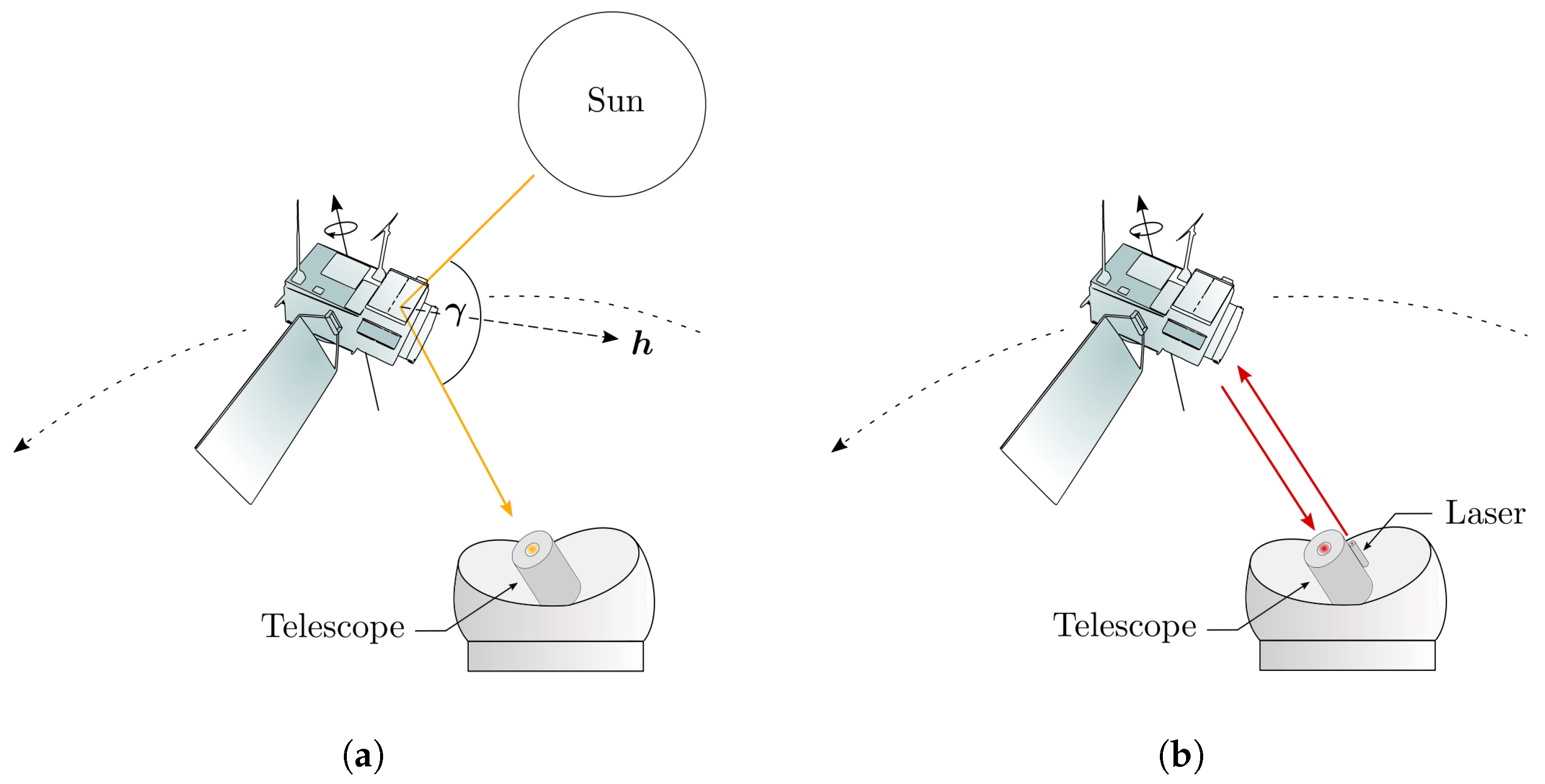
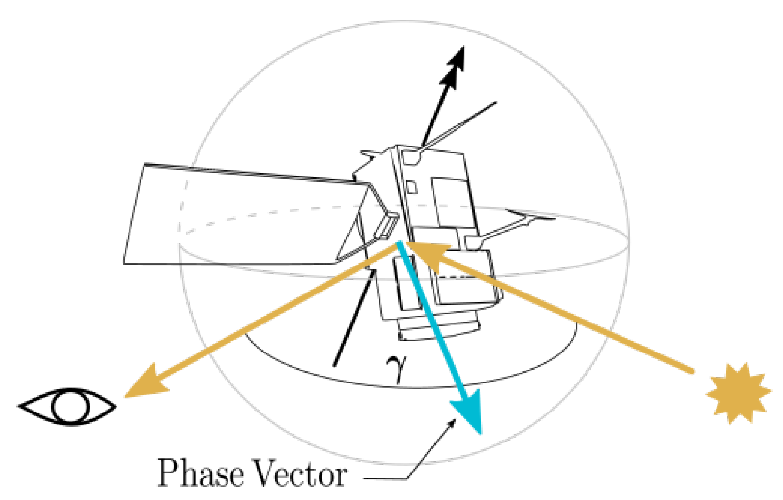
The circumstances at hand, thus, bring about the need for tools that provide reliable characterisations of objects in Earth’s orbit. A general approach to infer attributes from orbital targets has been to exploit ground-based observations, as measured light reflections vary based on an object’s orientation, shape and surface materials. Figure 1 depicts the geometric constraints of surveillances, where h represents the bisector of illumination and observation directions, also known as phase vector, and $\gamma$ is the angle between illumination and observation directions, referred to as phase angle. Typically, observations are obtained passively from sunlight reflections during local twilight [4]. Recent developments in satellite laser ranging provide prospects of conducting observations under active laser illumination, as demonstrated through laser ranging activities to non-cooperative targets [5]. Although signal returns are still comparably low, this method is of increasing interest, as it offers the potential for more accurate position measurements than radar, especially for smaller targets [5]. That being said, the distribution of returning photons is still poorly understood, which limits the accuracy of measurement to the radius of the object.

Previous studies have indicated that ground-based observations can provide the means to estimate targets’ shape, surface and rotation attributes [7,8]. However, due to the large parameter space dictating measured light reflections, signal inversion attempts are generally ill-posed. In addition, physical restrictions introduced by the atmosphere and the optical telescope aperture typically reduce observations to unresolved images. Especially for satellites at higher orbits (>1000 km), spatial resolution in images is for the most part insufficient to deduce attributes from spacecraft [7]. Consequently, observations are frequently compressed to time series of brightness measurements, known as light curves. The loss of spatial resolution further complicates the parameter estimation. For this reason, researchers often require a priori information and large datasets to be able to extract unknown attributes from targets. It is therefore expected that increasing the amount of independent measurements recorded for light curves through multispectral or polarised observations will benefit parameter extraction. Previous work has shown that the additional information provided by spectral and polarised measurements can improve the conditioning of the estimation problem and facilitate additional approaches to determine the surface composition of targets [9,10].

Satellite operators are reluctant to share information about their assets in space, so there is often no ground-truth information that could provide a basis for research on the parameter estimation from space debris. Physically accurate simulation can be a stand-in for ground-truth data. The simulation environment described in this paper will enable the development and testing of light curve inversion algorithms. The platform is validated through a comparison to a series of multispectral field measurements obtained in November 2020 using the DLR facilities at Uhlandshöhe research observatory. Further, parameter estimation approaches are demonstrated based on output from the simulator. The paper is concluded by discussing products of spectral simulations in context of their contribution to the inversion of light curve signals.

2. Literature Review

Software for the simulation of spectral light reflections from spacecraft has been presented in multiple publications so far. Probably the most frequently referenced of these is the Time-domain Analysis Simulation for Advanced Tracking (TASAT) [11] created by the U.S. Air Force Phillips Laboratory. Further approaches that can be found in published literature include the Digital Imaging and Remote Sensing Image Generation (DIRSIG) suite [12] of the DGIRS Laboratory at Rochester Institute of Technology and the CanCurve software [13] introduced by Willison and Bédard. Each of these simulators relies on Computer Aided Design (CAD) spacecraft models and the notion of the Bidirectional Reflection Distribution Function (BRDF) (see Equation (1)) to model light reflections [13,14,15]. A main difference between implementations thereby lies in the characterisation of material BRDFs. TASAT, for instance, features an empirical material database combining reflection models to compensate for sparse measurements [14]. However, a study by Wellems et al. points out shortcomings of this database being the limited amount of measurement samples for materials, both in spectral and geometric domains [16]. Moreover, research by Dugging et al. raises questions about the accuracy of the Maxwell-Beard BRDF model [17] used by TASAT, particularly when applied to specular materials [14].

The demonstration of DIRSIG’s simulation pipeline by Bennett et al. indicates that DIRSIG does not natively support reflection measurements [15], but rather relies on the parametrised Ward model [18]. By fitting the Ward BRDF to empirical measurements, Bennett et al. show that the model also entails increasing imprecision for specular materials [15].

Willison and Bédard strive to solve issues arising from BRDF models by supplying tabulated BRDF data directly to the CanCurve utility [13]. Their research suggests that this may help avoid errors of reflection models, although they acknowledge that their measurements lack sufficient and well allocated samples [13,19]. Consequently, inaccurate representation of an objects’ appearances cannot be excluded using current approaches, especially when considering the predominantly specular nature of frequent surface materials used on spacecraft, such as Multi-Layer Insulation (MLI) or solar panels [20,21].

Possibly the main shortcoming of simulators is the lack of quantitative and time-resolved validation to field measurements. For the TASAT software, Luu et al. attempt to compare simulations to full spectra taken from the cylindrical Galaxy V satellite [7]. Whilst empirical and synthetic data appear similar, the limited spectral range of observations is insufficient to correlate any significant features [7].

An image obtained from DIRSIG is opposed to an observation from the 3.6 m AEOS telescope in Hawaii by Bennett et al. [15]. However, no validation of temporal or quantitative results of the simulation are included in the document [15].

Simulated reflections using CanCurve are compared to ground truth measurements collected by Bédard et al. in [22] from the CanX-1 CubeSat [13]. The simulation model is thereby constructed from BRDF measurements of white paint, aluminium and the CanX-1 solar cells [13,20]. Modelled and empirical spectra are shown to possess similar features at multiple observation directions. Regardless, no quantitative comparison can be drawn between them, as measurements are recorded in sensor counts while simulated results are only computed as spectral BRDF values. Moreover, the comparison does not include atmospheric effects encountered during ground-based observations.

Examining the presented software highlights the need for a solution that combines accurate measurements of material reflections with a physically sound simulation environment. Moreover, the focus of developments should be placed on the accuracy of predictions and facilitating parameter estimation. Therefore, a refined approach should strive to attain a quantitative comparison to field recordings of light curves to assess the validity of the model.

3. Materials and Methods

The simulation framework presented in this paper is built on the Raxus Prime light curve simulator, which was originally implemented by Daniel Burandt [23] at the Institute of Technical Physics of the German Aerospace Centre (DLR) in Stuttgart. Former revisions to Raxus Prime were carried out by Ewan Schafer [24], which form the basis for this research. Up until now, Raxus Prime relied on the POV-Ray render engine [25] to determine light transport. Consequently, simulations were restricted to monochromatic renders of relative brightness values that were not related to physical units of radiance. Thus, computations could not fully represent ground-based satellite observations, which are subject to wavelength dependent material reflections and atmospheric attenuations. Nevertheless, Burandt et al. were able to produce comparable light curves to measured data by optimizing targets’ rotation parameters [26], thereby supporting the notion of utilizing available render software to model reflections. At the same time though, the results of Burandt et al. highlight the complexity of validating the simulation environment, as for most targets, insufficient information is accessible, introducing large uncertainties within the replicated scene.

An enhanced version of Raxus Prime is therefore presented that overcomes previous limitations by including wavelength-related effects of radiation transfer and allowing spectrally accurate instrument transmissions and detector quantum efficiencies to be considered. The new simulation pipeline is novel in its ability to generate radiometrically correct multispectral light curves of satellites in arbitrary wavelength bands as they would be observed on the ground, even when non-standard spectral bands are used for observation. This is critical for photon-starved applications, such as high time resolution satellite photometry, where optical elements such as dichroic mirrors with non-standard transmission and reflection spectra are employed to maximise the sensitivity of the system.

The use of open-source software components contributes to the computational efficiency of the tool and gives access to features that have previously not been available to light curve simulators, including differentiable rendering and ingesting state of the art formats for tabulated reflection measurements. The following section covers the necessary adjustments to facilitate spectrally resolved simulations. 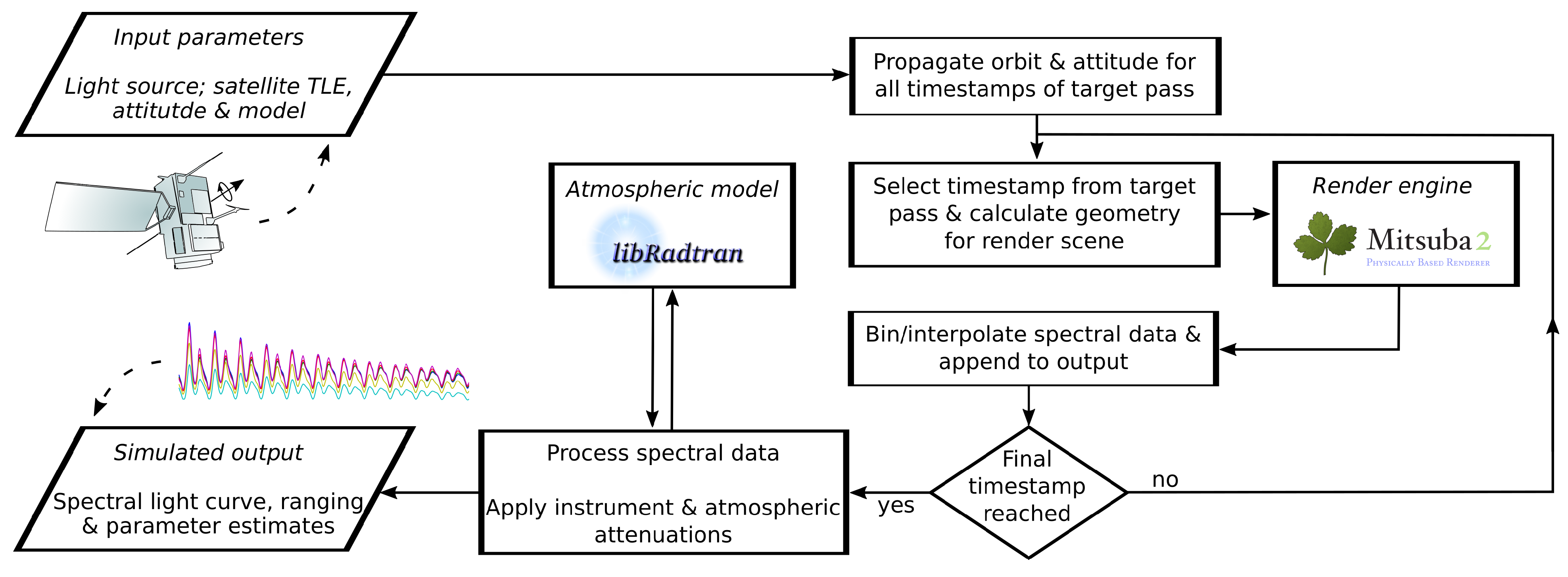Figure 2 visualises the updated simulation pipeline.

To model a satellite observation, Raxus Prime requires a set of input parameters defining the satellite’s reflectance and motion as well as the location of the observer. Specifically, the input includes:

• The target’s orbital Two-Line Element (TLE) for propagating the satellites trajectory;
• Initial attitude and rotation parameters of the target, including inertia tensor, rotation axes and rotation periods;
• A 3D target model, partitioned based on material representations using the BRDF reflection model;
• Observer location in geocentric coordinates.

For active laser ranging scenarios, at least one transmitter is specified from a location, beam divergence and power spectrum. Optionally, simulated products can be customized by supplying optical transmissions and efficiencies of the receiver instruments. Raxus Prime also provides a selection of generic satellite shapes, reflection models and beam profiles that can be useful if these details are not known beforehand.

The simulation is carried out in three principal steps:

• Geometric relations between light source, target and observer are propagated from a target’s TLE and rotational parameters. Alternatively, positions can be set manually, using information from, for example, Consolidated Prediction Format (CPF) format predictions;
• Reflections are computed by rendering the geometry at discrete time intervals during the pass and subsequently fused to form a spectral light curve;
• Additional processing steps are applied to the series of spectral data such as atmospheric attenuation or conversion to instrument responses.

TLE propagations are performed using the Simplified General Perturbations 4 (SGP4) model, which can be accessed at [27]. The target attitude is calculated from the torque free Euler equations [24,26], under the premise that its rotation state remains constant. In most cases this is a valid assumption, as typical values for environmental torques acting on objects in Earth orbit are on the order of 10⁻⁴ to 10⁻⁷ Nm [28,29,30], which are too small to have a significant effect on the objects’ rotation over the time span of a simulated pass (usually less than 10 min). Analysis of historical spin periods for satellites such as TOPEX/Poseidon and Envisat have revealed changes in rotation periods of approximately 1.1 and 0.3 degrees per year, respectively [28,31].

3.1. Spectral Renders

Following the example of previous versions of Raxus Prime, the spectral simulation pipeline harnesses the capabilities of specialised render software. Spectral renders are performed using the Mitsuba2 open-source render engine [32], which implements a classical Monte Carlo ray tracer, featuring a range of sampling strategies to ensure the efficiency of computations. Mitsuba2 is also capable of modelling polarised light and can be adapted to render scenes in a fully differentiable fashion [32]. Although these features are not yet supported by Raxus Prime, they provide promising areas for further developments.

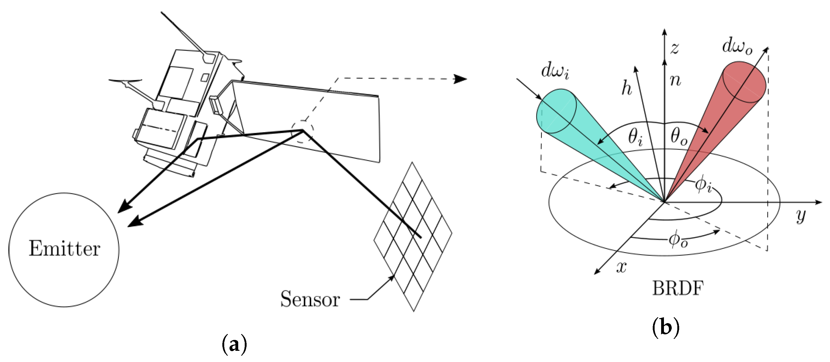
Figure 3a depicts the principle of Mitsuba’s ray tracing algorithm. Rays are cast from the sensor and intersected with the scene geometry. At each intersection, the scattering model of the surface material is evaluated to determine the attenuation along the ray and sample further directions of incident light. Scattering properties of surfaces are generally characterised by the Bidirectional Scattering Distribution Function (BSDF), which accounts for effects of reflective as well as transmissive materials [33]. It was determined by means of visual inspection that common spacecraft materials such as solar panels, MLI or aluminium permit little subsurface transmission. Therefore, light interactions are captured solely through reflective effects using a subset of the BSDF, namely the BRDF. The BRDF is defined as the ratio of reflected radiance $L_o({\omega }_o,\lambda )$ to incident irradiance $E_i({\omega }_i,\lambda )$ on a surface [33], ergo

$$f_r({\omega }_i,{\omega }_o,\lambda )=\frac{d{L}_o({\omega }_o,\lambda )}{dE({\omega }_i,\lambda )}·\left[{\mathrm{sr}}^{-1}\right]$$

(1)

The distribution of surface reflections, thus, makes up a five-dimensional problem that varies with the wavelength $\lambda$ as well as directions of incident ${\omega }_i$ and outgoing ${\omega }_o$ light; see Figure 3b. In particular cases, such as isotropic materials or Lambertian surfaces, the parameter space can be reduced to four [34] or one dimensions [33], respectively. For fully diffuse objects, reflections are characterised by the surface albedo ${\rho }_g\left(\lambda \right)$ and are independent of the lighting geometry [33].

Before interfacing Mitsuba2 from the Raxus Prime environment, the render process was modified to extract spectral data directly, rather than converting to RGB images first. A custom scene integration procedure was implemented using the Python bindings of Mitsuba2, so that the main rendering tasks are still delegated to Mitsuba’s C++ functions. The integration relies on a stratified sampling approach to draw random wavelengths samples for each ray. Upon rendering a scene, the spectral output is binned to form hyperspectral intensity maps that can be stored for later processing. The data is saved in units of [$\mathrm{W}/{\mathrm{sr}}^{-1}/\mathrm{n}{\mathrm{m}}^{-1}$], allowing for subsequent scaling by the measurement aperture to determine the expected spectral flux at the telescope.

Although the spectral range of renders is technically not restricted, Mitsuba2 assumes radiation transfer to occur in thermal equilibrium, thereby ignoring any influence of thermal emission. Hence, the accuracy of computations will degrade towards infrared wavelengths, where thermal effects contribute significantly to radiation transfer [35]. For this study, simulations were limited to wavelengths ranging from 300 to 1240 $\mathrm{n}$$\mathrm{m}$ at a resolution of 5 $\mathrm{n}$$\mathrm{m}$.

Target models for Mitsuba can be created using the OBJ and PLY standard 3D-model formats. Reflection models need to be assigned individually to each target component. Models are drawn from standard distributions, which include options for specular, diffuse or GGX [36] or Beckmann [37] surfaces. Spectral scattering distributions of materials can be altered based on the Fresnel equations by supplying refractive properties [32] or by overlaying predefined reflectance spectra. Alternatively, measured BRDFs using the adaptive sampling method introduced by Dupuy and Jakob in [38] can be sourced from their database [39] or specified independently. 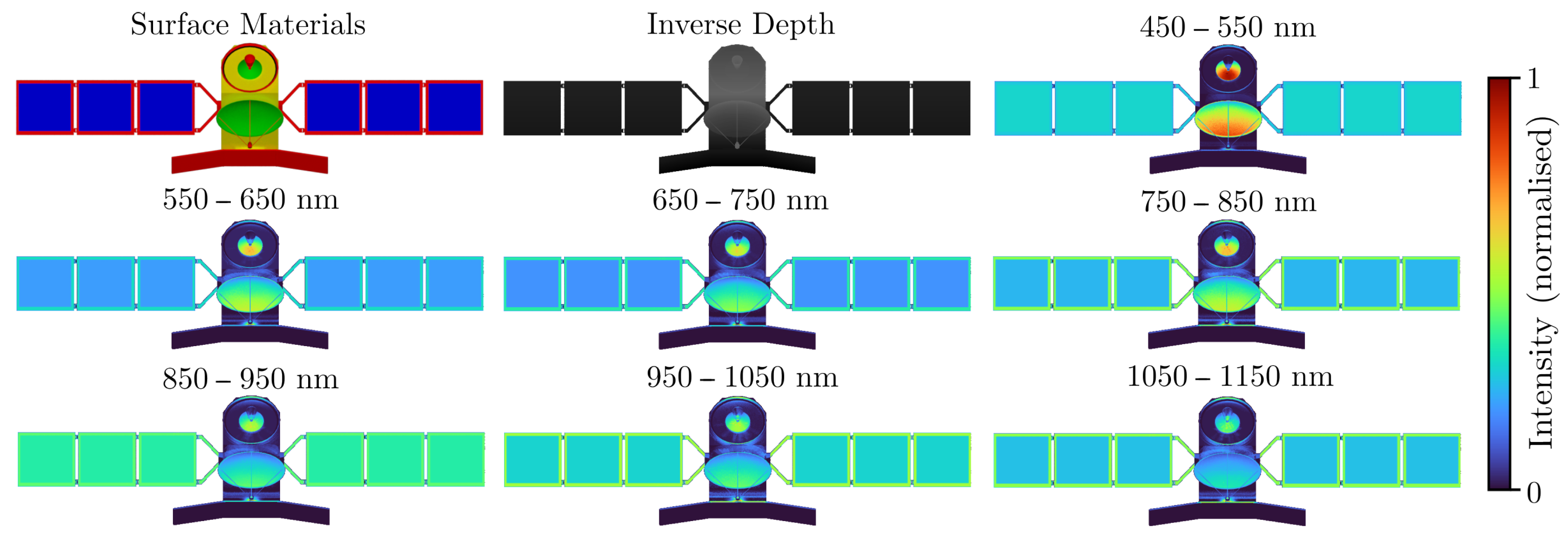Figure 4 gives an example of the varying appearance of a target across separate spectral bands, based on renders of a box-wing satellite. In this case, diffuse and Beckmann BRDF models were combined with lab measurements of reflectance spectra taken at a single illumination and scattering configuration; further details are given in [21].

Satellite observations require a relatively simple render scene consisting of the target model, a sensor and one or more transmitters corresponding to the Sun and/or lasers. For simplicity, transmitters are modelled using parallel light sources and an orthographic sensor model, which was ported from the previous version of Mitsuba to represent the telescope. It was found that the small divergence of ranging lasers, which is typically in the range of several arcseconds, is negligible for renders, as it is generally well below the accuracy of material reflection measurements. The same applies to the change in perspective induced by the orthographic sensor due to the relatively small cross section of targets and the large distance between target and observer for ground-based observations. In contrast, the Sun’s angular diameter seen from a satellite is ∼0.54 degrees, which may have a detectable influence on reflections from highly specular materials, for which slope widths of specular peaks were observed down to approximately one degree while obtaining lab measurements for this paper. Minor angular differences must therefore be considered when evaluating specular sunlight reflections.

Each transmitter in the render scene is instantiated from a spectral irradiance distribution. The solar irradiance in Earth’s orbit is determined from measured spectra collected in the libRadTran library [40,41], which is introduced in the following section. Laser irradiance on a target is calculated from an emission spectrum and the general laser and geometric parameters, including beam divergence, distance to the object and average power output.

3.2. Post-Processing

Atmospheric effects are accounted for by the radiative transfer library libRadtran [40,41], which was developed as open-source software at the DLR in Oberpfaffenhofen. Raxus Prime exploits the library to compute transmission spectra in the wavelength resolution of the render at each observation geometry. Atmospheric attenuation, thus, varies with the location of the observer and local target elevation. Turbulence related effects, such as atmospheric scintillation, are currently not considered, as image blurring and statistical fluctuations are not relevant for non-resolved observations when measurements are averaged over time spans larger than the respective coherence time [35]. Static losses are considered during the calibration of reference measurements.

Rendered spectra are multiplied by the atmospheric transmission to determine the spectral intensity of light at the telescope. For active illumination, incident laser light on the target is weighted equivalently.

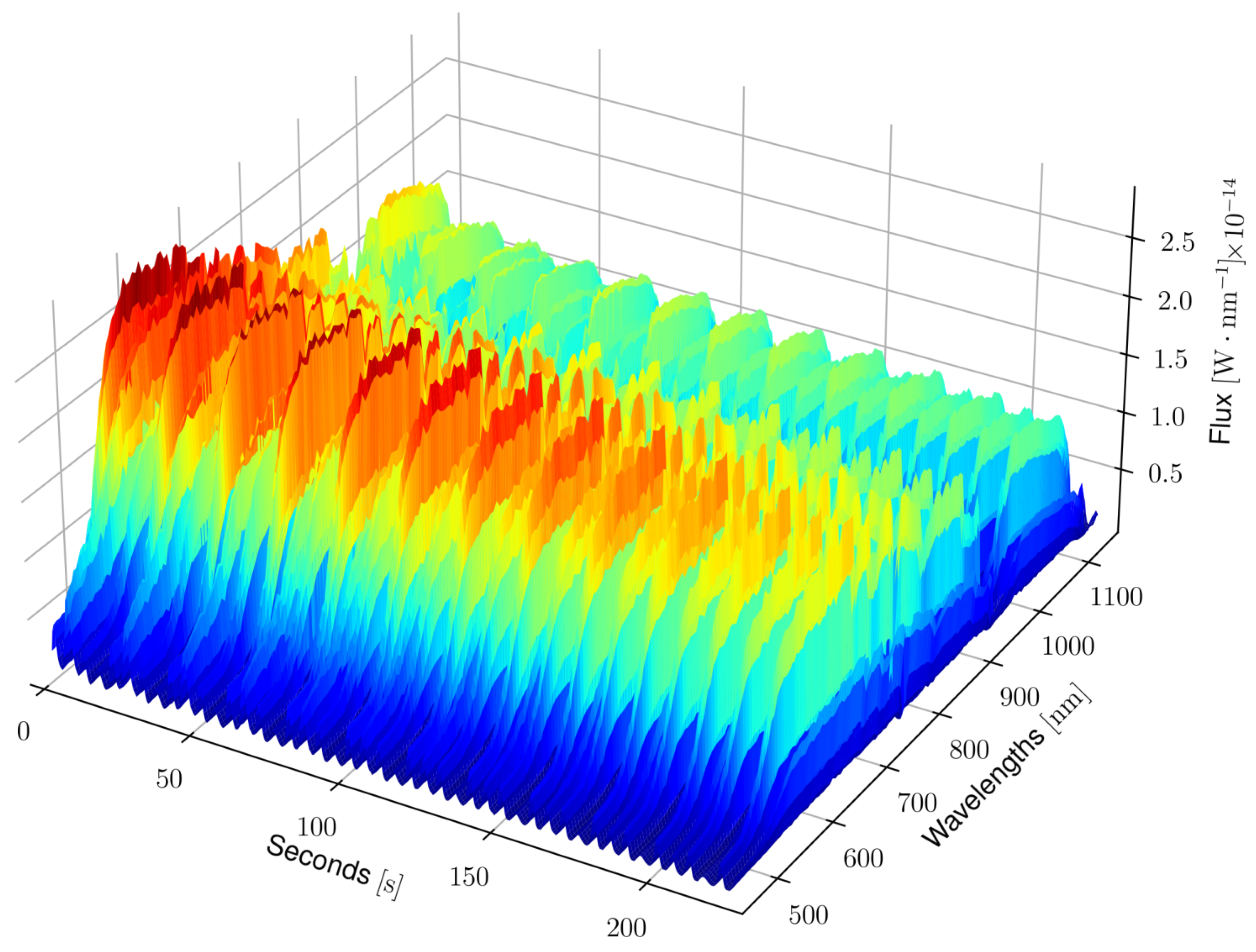
Hyperspectral images from the render can be fused to a single spatial point to form spectral light curves. In this case, the spectral flux $\Phi \left(\lambda \right)$ at the telescope is determined by summing rendered intensity maps over all pixels and multiplying with the observational solid angle, so that

$$\Phi \left(\lambda \right)=\sum _p{\overline{I}}_p\left(\lambda \right)\frac{A}{r^2}.$$

(2)

where, ${\overline{I}}_p\left(\lambda \right)$ is the average intensity spectrum at each pixel p of the orthographic sensor and the solid angle is defined as $A/r^2$, where A is the cross section of the telescope aperture and r the distance between target and observer. An example of a synthetic spectral light curve, produced by Raxus Prime, is given in Figure 5.

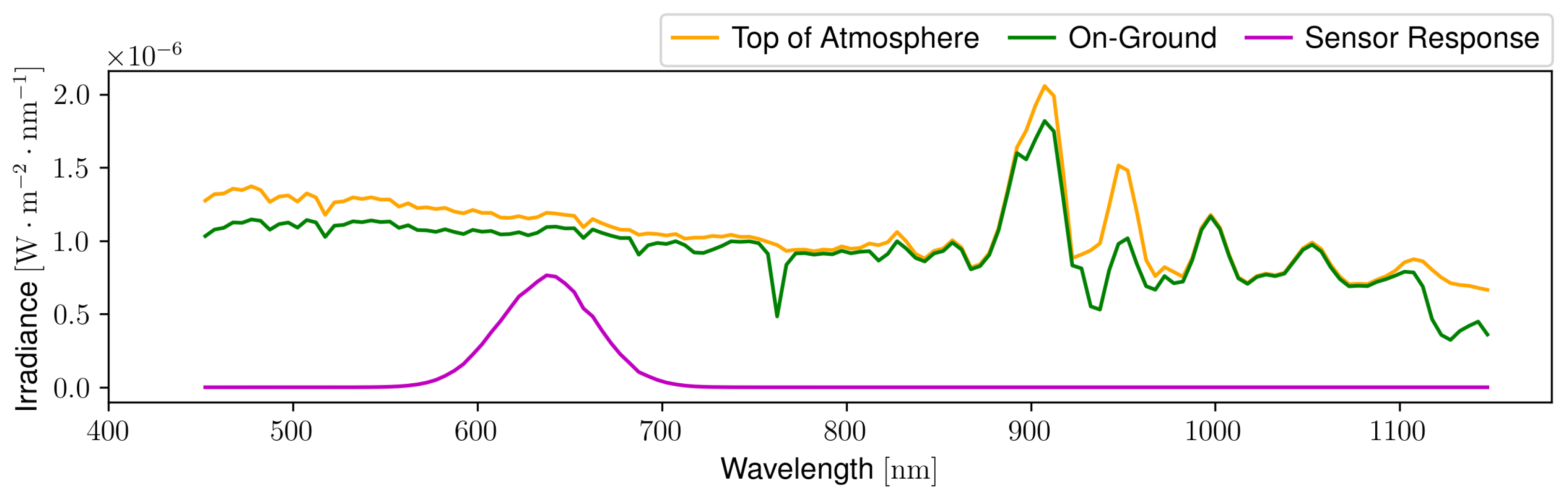
Simulated instrument responses are the product of spectral light curves, transmission spectra of the telescope optics and instrument specific efficiencies, integrated over the wavelength range of optical throughput. Figure 6 gives an impression of the processing steps involved in converting a rendered spectrum to an instrument response for a single observation geometry.

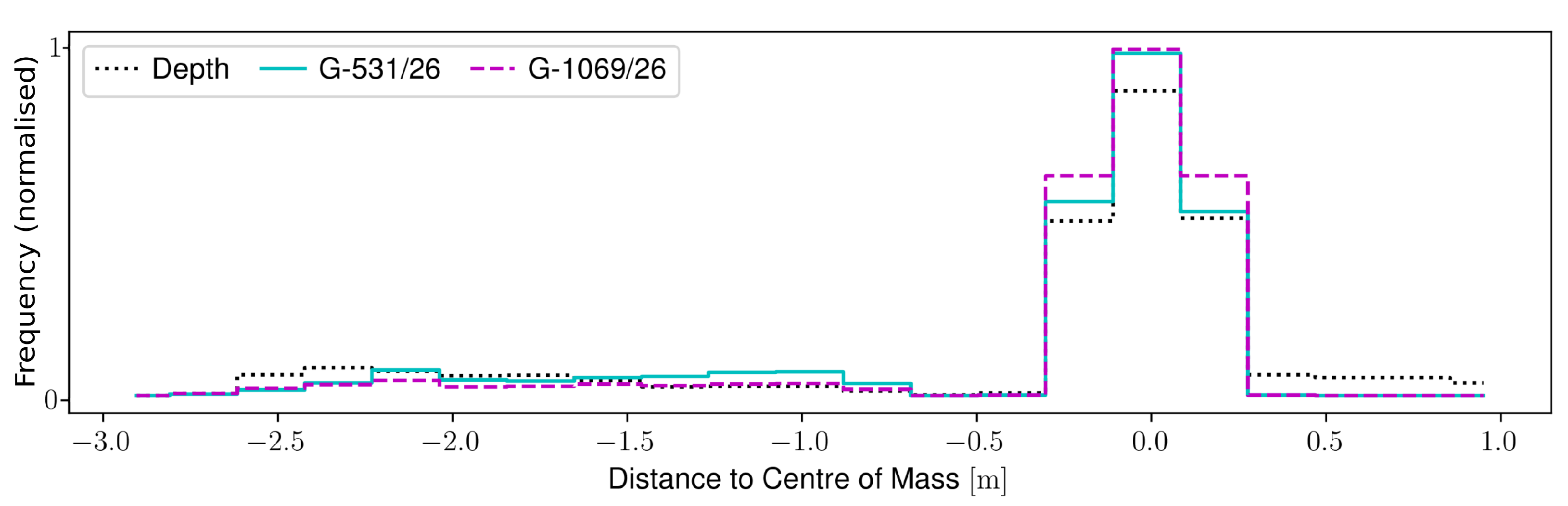
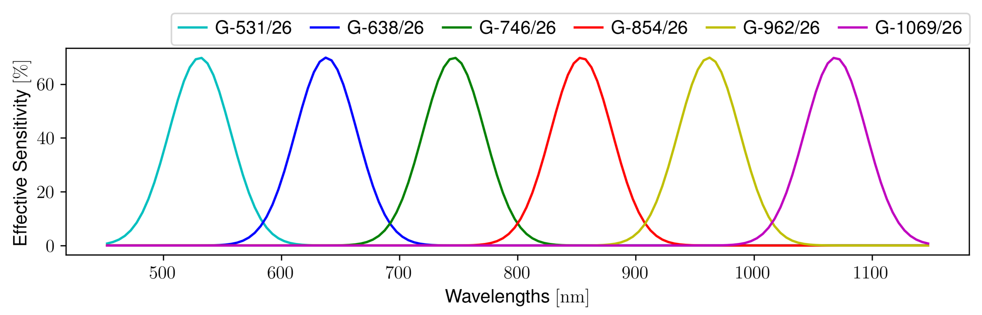
Laser ranging to non-cooperative targets is modelled by applying atmospheric and instrument attenuations directly to the hyperspectral intensity maps produced by the render. Using the resulting distribution as weights for the depth map of the rendered scene, the statistical distribution of photon returns can be evaluated. Figure 7 depicts the normalised ranging histogram for the scene in Figure 4. Observation bands are chosen to be generic Gaussian curves with centre wavelength λ and standard deviation σ, so that G-${\lambda }_{\mathrm{centre}}$/σ.

Examining the simulated data reveals that the required centre of mass corrections for ranging estimates differ across observation bands. This is a consequence of the varying spectral reflectivity among visible surface materials. Offsets will differ based on the sensor band, observation direction and surface properties of the target. Theoretically, this limits the accuracy of measurements to the object’s radius if no further target information is known. For the given example, the distance from the satellite’s true position and the averaged range measurements in each band are ∼$0.05$ $\mathrm{m}$ in the G-531/26 and ∼$0.01$ $\mathrm{m}$ in the G-1069/26 band. That being said, it should be noted that the simulation method does not yet account for repeated reflections on the target.

4. Results

Due to the large parameter space of observations, validating the simulation environment is not trivial. To gather suitable reference data, it is essential that the number of unknown parameters is constrained to a minimum. In spite of this, satellite providers generally do not publish details concerning the attitude or surface properties of their spacecraft. Further, the appearance of objects has been found to change when exposed to the space environment for extended periods of time [42]. Consequently, the main issue lies in determining targets for which the relevant information is accessible.

An equivalent problem is encountered during the calibration of radar stations. For this purpose, governmental institutions have launched a range of passive calibration targets into Earth’s orbit. While obtaining reference measurements for this research, the two spherical satellites listed in

Table 1. Observed radar calibration spheres. Parameters were obtained from [43].

Satellite	NORAD ID	Surface Material	Diameter [m]
Calsphere 4A	1520	White paint	0.36
Lincoln Calibration Sphere 1 (LCS 1)	1361	Polished aluminium	1.13

were recorded. Each of these is made from a uniform surface material; therefore, their attitude does not influence observations. Although precise surface specifications are not publicly obtainable, the general material category allows for the objects’ reflectance to be estimated within reasonable bounds.

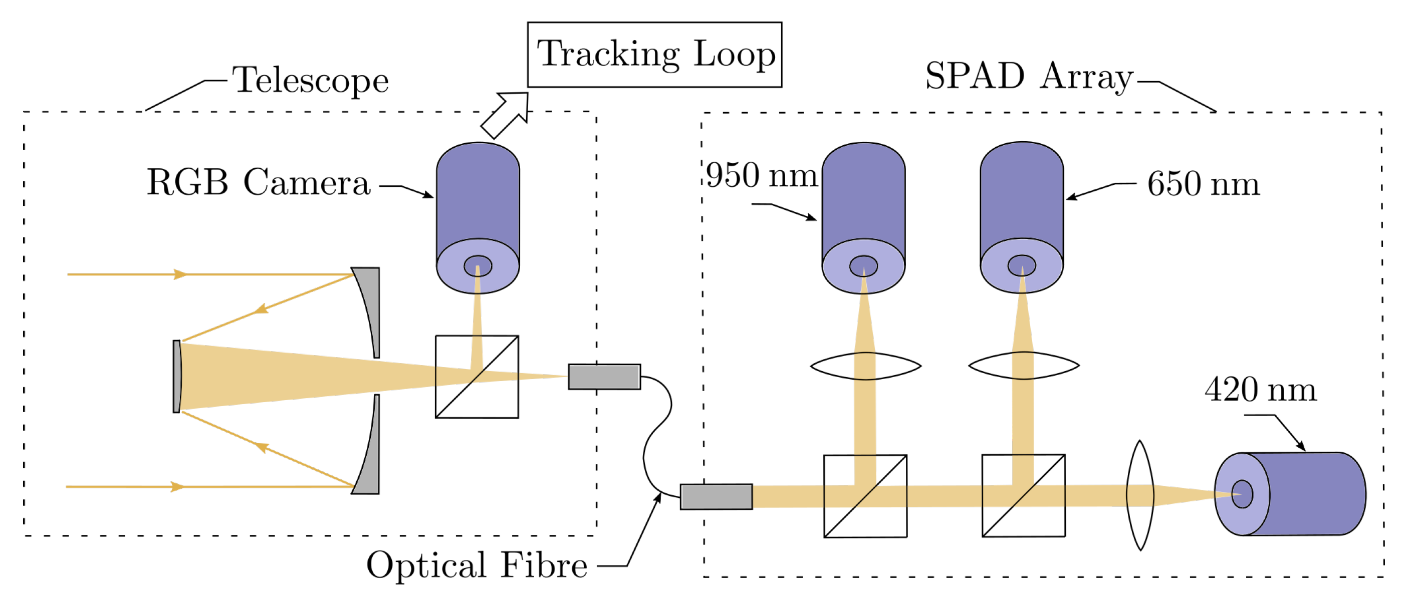
Reference data was collected at the Uhlandshöhe research observatory using a corrected Dall–Kirkham telescope with a primary mirror diameter of 43 $\mathrm{c}$$\mathrm{m}$ and a focal length of 3 $\mathrm{m}$. The optical setup is depicted in Figure 8. Multispectral recordings were obtained from an Atik 414ex RGB camera and three Single-Photon Avalanche Diodes (SPAD) with peak efficiencies at 420, 650 and 950 $\mathrm{n}$$\mathrm{m}$. The instruments were calibrated based on a series of star observations throughout each night of observation to facilitate a quantitative comparison between measured and simulated light curves. For details on the optical system and calibration, the reader is referred to [21].

The limited size of the telescope aperture meant that reflections from Calsphere 4A were for the most part below the signal-to-noise threshold for the instruments. Because of that, only one pass was recorded for which the signal in the 950 $\mathrm{n}$$\mathrm{m}$ SPAD did not exceed the noise threshold. LCS 1 generally appeared brighter, so that three clear passes during two nights of observation were acquired.

Previous observations by Hall et al. have shown Calsphere 4A to appear almost fully diffuse, while LCS 1 is largely specular in reflections [43]. Hence, for simulations, Calsphere 4A was modelled using a diffuse BRDF and LCS 1 was assigned surface properties based on the isotropic Beckmann model, which combines specular and diffuse reflections through an additional roughness parameter. In both cases, the exact spectral reflectance was unknown and had to be determined by fitting synthetic to measured light curves. For LCS 1, the roughness parameter required for the Beckmann model was included in the estimation.

Optimisations of synthetic data were performed over a set of attenuation factors in each of the observation bands using the constrained Sequential Least SQuares Programming (SLSQP) algorithm [44]. To simplify computations, count rates from the single photon detectors were binned to match the frequency of camera images.

Table 2. Fitted simulation parameters based on observed passes in the RGB camera and Single Photon Avalanche Diodes (SPAD).

Satellite	Model	Roughness	Band Albedo
		$\mathit{\alpha }$	R	G	B	950 nm	650 nm	420 nm
Calsphere 4A	Diffuse	-	0.75	0.73	0.70	-	0.76	0.86
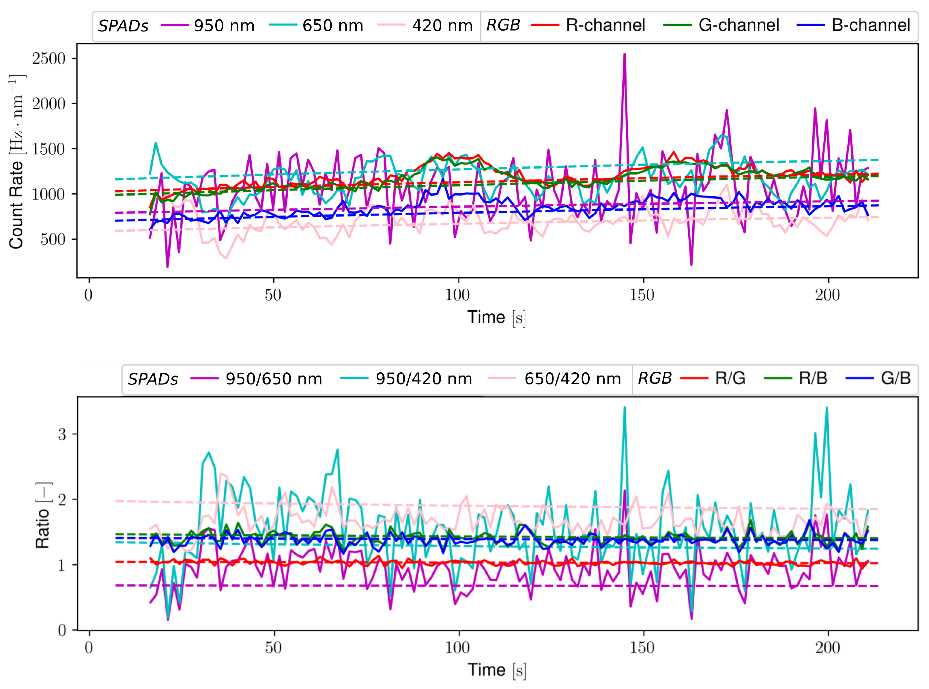
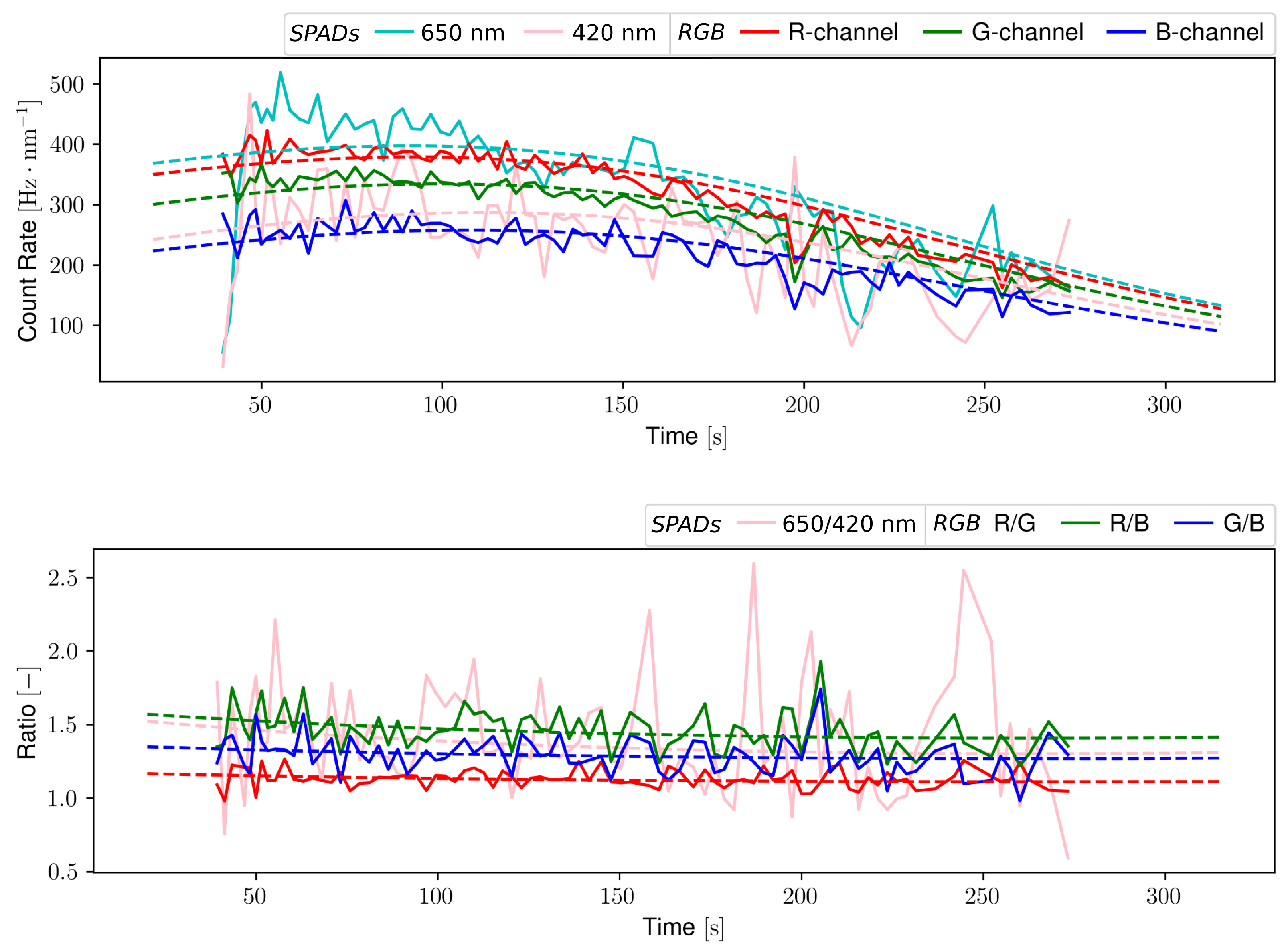
LCS 1	Beckmann	0.12	0.67	0.73	0.66	0.72	0.73	0.63

gives an overview of the extracted albedo coefficients for Calsphere 4A and LCS 1. The comparison between simulated and measured light curves can be seen in Figure 9 and Figure 10. Although the measurements are subject to noise, synthetic and empirical data are overall in agreement, which is underlined by RMS errors of less than one percent with respect to the total measured signal counts. The signal ratios further indicate that the simulation correctly captures the influence of varying atmospheric attenuation along the targets’ trajectories. Comparably high fluctuations detected for LCS 1 are corroborated by observations of Hall et al. and are most likely a consequence of surface irregularities leading to alterations in the specular reflection from the target [43].

5. Discussion

Products of the simulation can be exploited to study the general inversion problem in detail. The main benefit of having a software environment to model space debris observations lies in the flexibility of modelled scenarios and its capability to generate large amount of data. To demonstrate this, several approaches are discussed that rely on synthetic light curves to determine target aspects. Presented procedures are included in the Raxus Prime simulation environment as optional post-processing steps.

5.1. Spectral Upsampling

When re-examining the fit of simulated to observed light curves from the previous section, it is possible to derive further properties of the calibration spheres. As both targets have uniform surface materials, fitted albedo values constitute low resolution reflectance signatures. Hence, the targets’ reflectance spectra can be estimated by applying spectral upsampling techniques.

Assuming that observations were conducted in n bands with spectral sensitivities $P_0\left(\lambda \right),P_1\left(\lambda \right),\dots ,P_{n-1}\left(\lambda \right)$, then any spectral distribution $g\left(\lambda \right)$ matching observed albedo values $\rho =[{\rho }_0,{\rho }_1,\dots ,{\rho }_n]$ must satisfy

$$\widehat{g}\left(\lambda \right)=arg\underset{g}{min}∥\rho -\frac{\int g\left(\lambda \right)P\left(\lambda \right)\lambda d\lambda }{\int P\left(\lambda \right)\lambda d\lambda }∥.$$

(3)

Here, $P\left(\lambda \right)=[P_0{P}_1\cdots P_{n-1}]$ represents the matrix of spectral sensitivity functions in each band. Further, band specific bias is avoided through normalising by the photon throughput in each observation band $P\left(\lambda \right)\frac{hc}{\lambda }$, where h is Planck’s constant and c is the speed of light in vacuum.

For this study, an upsampling method presented by Jakob and Hanika [45] was expanded to accept multispectral input in arbitrary spectral bands. The original method employs a second order polynomial smoothed by a sigmoid function to approximate spectral distributions from tristimulus values [45]. The sigmoid function $S\left(x\right)$ is defined so that it projects the range of polynomial estimates $[-\infty ,\infty ]$ to values between 0 and 1, with

$$S\left(x\right)=\frac{1}{2}+\frac{x}{2\sqrt{1+x^2}}.$$

(4)

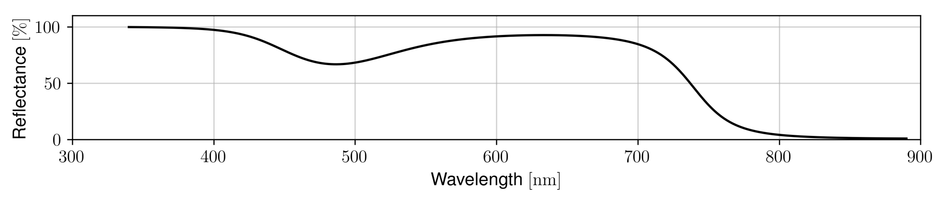
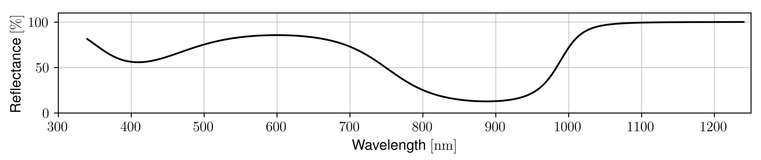
Transferring this idea to n-dimensional observations permits the use of polynomial estimates of order $n-1$. Figure 11 and Figure 12 show this applied to the extracted albedo coefficients of Calsphere 4A and LCS 1, respectively. It will be noted that solutions only represent suggested spectra, as any upsampling is inherently underconstrained. Nevertheless, the identified reflectance of Calsphere 4A is similar to measurements of artificially weathered thermal control paints gathered by Bengston et al., for which reflectivity dips around 500 or 600 $\mathrm{n}$$\mathrm{m}$ and generally declines towards higher wavelengths [46]. It is expected that the steep decrease in reflectiveness starting at 700 $\mathrm{n}$$\mathrm{m}$ is an artefact of the sigmoid function combined with reduced detector sensitivity around 900 $\mathrm{n}$$\mathrm{m}$.

The spectrum obtained for LCS 1 reveals characteristics of other aluminium spectra found in [20], including a general gain in reflectiveness towards larger wavelengths and dips around 400 and 800 $\mathrm{n}$$\mathrm{m}$. Even so, both dips are more prominent than in the literature and the latter appears slightly shifted towards 900 $\mathrm{n}$$\mathrm{m}$, which may also be traced back to the decreased sensitivity of the observation set-up around 900 $\mathrm{n}$$\mathrm{m}$.

5.2. Spectral Unmixing

Advantages of spectral observations become apparent when examining signal variations across individual measurement channels. For one, independent channels can help reduce ambiguities in the parameter estimation [10,21]. Primarily though, spectral signatures can be used to discriminate between targets and discern their material properties [7,47,48,49,50].

Essentially, light curves are defined by the emission spectrum of the light source and scattering properties of the target’s surface materials, as well as atmospheric attenuation effects for ground-based observations. Since solar or laser emission profiles are known and atmospheric transmission has been well classified, observed signals can be reduced to the target’s reflectance signature. The resulting quantity constitutes the combined reflective properties of all the target’s surface materials that contribute to a reflection.

Let ${\Gamma }_j$ be a target’s reflectance factor in an observation band j; then

$${\Gamma }_j=\frac{{\Phi }_{o,j}}{{\Phi }_{i,j}},$$

(5)

where ${\Phi }_{o,j}$ refers to the measured flux at the telescope and ${\Phi }_{i,j}$ is the incident flux on the target, which can be determined from the spectral energy distribution of the light source. For ground-based observations, ${\Phi }_{o,j}$ includes atmospheric attenuations. These can be removed from the reflectance factor by applying the atmospheric transmission profiles while calculating ${\Phi }_{i,j}$.

If measurements are carried out within multiple spectral bands, a system of equations can be established that describes the target’s reflectance signature as a mixture of the reflectance of its individual surface materials. Fortunately, surface materials on artificial satellites are typically segregated in discrete patches, so that a linear mixing model can be assumed [51], taking the form of

$$x=Sa+w.$$

(6)

Here, x denotes a measured spectrum of n samples, S is an $(n\times m)$ matrix containing the spectral signatures of m materials, a quantifies the signal contribution of each material and the noise term w captures any inhomogeneities of the model. By minimising the noise term, the model can be turned into an optimisation problem yielding the contribution vector a. The signal contribution is also referred to as abundance; however, this term can be misleading, as the representation of material signatures within a reflection is dependent on the materials’ reflective properties as well as the size of the reflecting surface area.

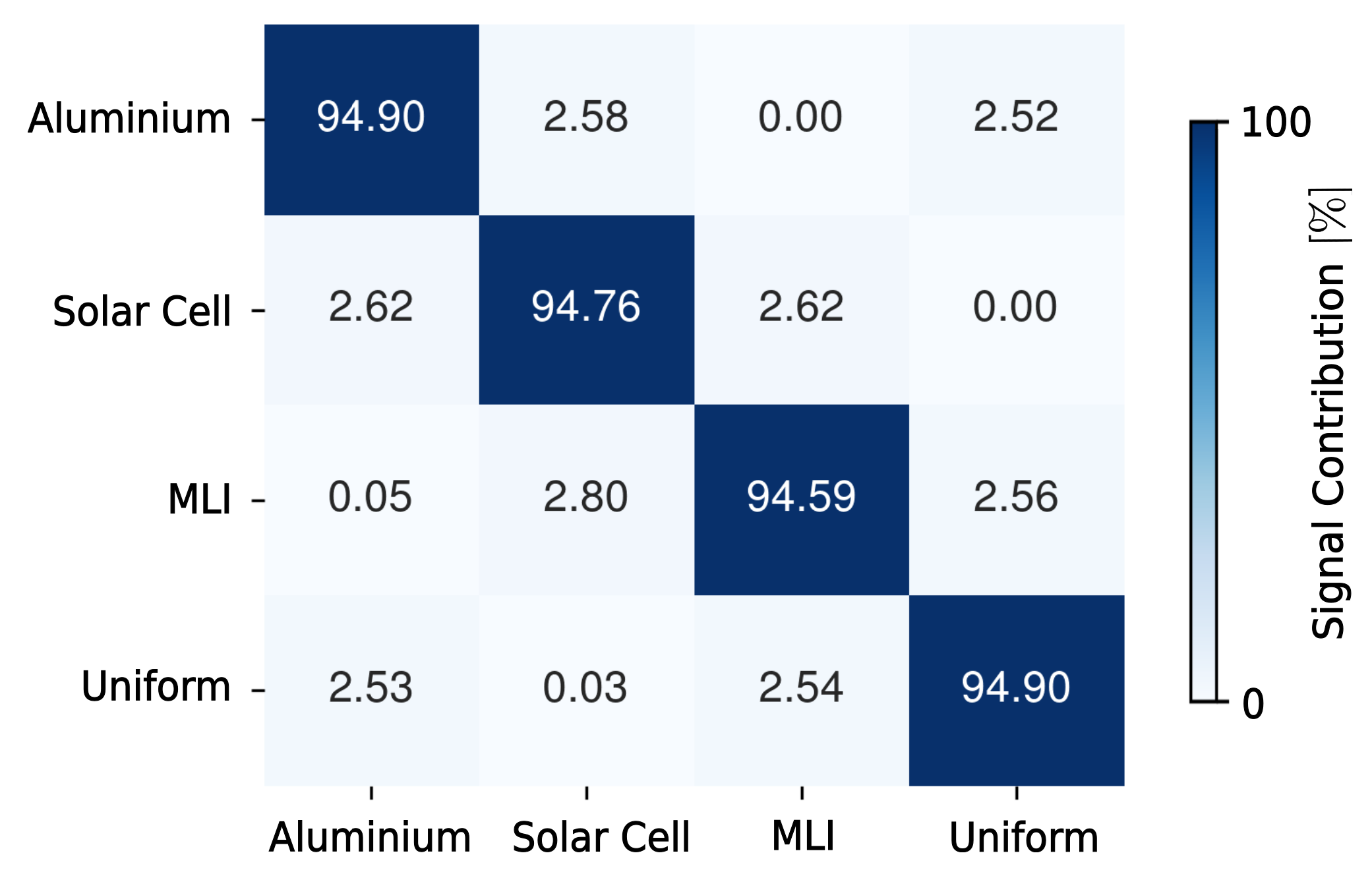
For an initial demonstration of the unmixing algorithms, simulation models were constructed from diffuse and Beckmann BRDFs with manually imposed spectral reflectances. Lab measurements of reflectance spectra from a solar cell, Kapton-coated MLI and aluminium were obtained in the clean room environment at the DLR Institute of Technical Physics in Stuttgart. Additionally, a uniform distribution was added to roughly resemble white paint. Three different least squares algorithms were tested to extract the contribution vector for the given spectral signatures: unconstrained, non-negative and fully constrained least squares. It was found that the non-negative least squares method followed by a normalisation of the contribution vector performed best. Naturally, estimations relying on a large amount of spectral samples are more reliable. However, the observation bands depicted in Figure A1 of Appendix A proved sufficient to unmix the subset of studied materials. To simplify the ground truth predictions, simulations were performed on a rotating cube with sides corresponding to each of the four materials. The model was first placed under solar irradiation and then under simultaneous illumination by seven evenly distributed laser beams across the spectral range of the simulation. In both cases, the estimation performed equally well. Figure 13 indicates the resulting confusion matrix. Predictions proved comparably reliable to unmixing attempts documented by Hall et al. in [49,52].

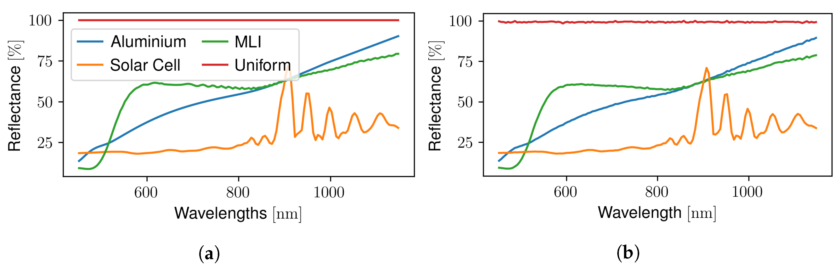
Unmixing signals from known spectral distributions requires a large spectral database that includes matching materials for all observed targets. Therefore, a more practical strategy is to extract source signatures directly from signals. Again, multiple approaches exist to achieve this, such as Principal Component Analysis (PCA) or the Automatic Target Generation Process (ATGP) [53]. Both algorithms were tested on simulated observations of the box-wing satellite model depicted in Figure 4. In this case, ATGP proved superior; while PCA was only able to extract linear combinations of the true material signatures; the results from the ATGP algorithm given in Figure 14 present a suited approximation of the objects’ surface materials. Minor fluctuations of simulated spectra are a result of Monte Carlo noise stemming from random sampling of the spectral domain.

5.3. Rotation and Attitude Estimation

A promising method used to gain more insight on targets’ surface composition and motion has been applied by Kucharski et al. in [54,55]. By projecting measurements onto a sphere in a target’s body frame, it is possible to create a reflection map of the target. Thereby, the position of measurements on the reflection map is defined by the orientation of the phase vector of each measurement with respect to the targets body frame; see Figure 15. To apply this method, prior knowledge of the target’s attitude throughout an observation is required. However, Kucharski et al. indicate that the mapping may be used to extract attitude and rotation parameters of targets, as the reflection map is shown to be smooth for correct estimates [54]. Accordingly, brute force optimisation can be applied to find a set of suited attributes [56].

Active, laser-based observations in which illumination and observation directions coincide ($\gamma =0^{\circ }$), produce unique reflection maps. For passive surveillance on the other hand, multiple observation configurations may correspond to the same phase vector; thus, the reflection map may differ slightly depending on the observation geometry. During one pass, however, observations are often restricted to a single observation geometry for each direction of the phase vector with respect to the targets’ body frame. Hence, maps produced from passive observations by Kucharski et al. are not affected by this. It remains unclear to what extent reflection distributions can be combined from separate passes.

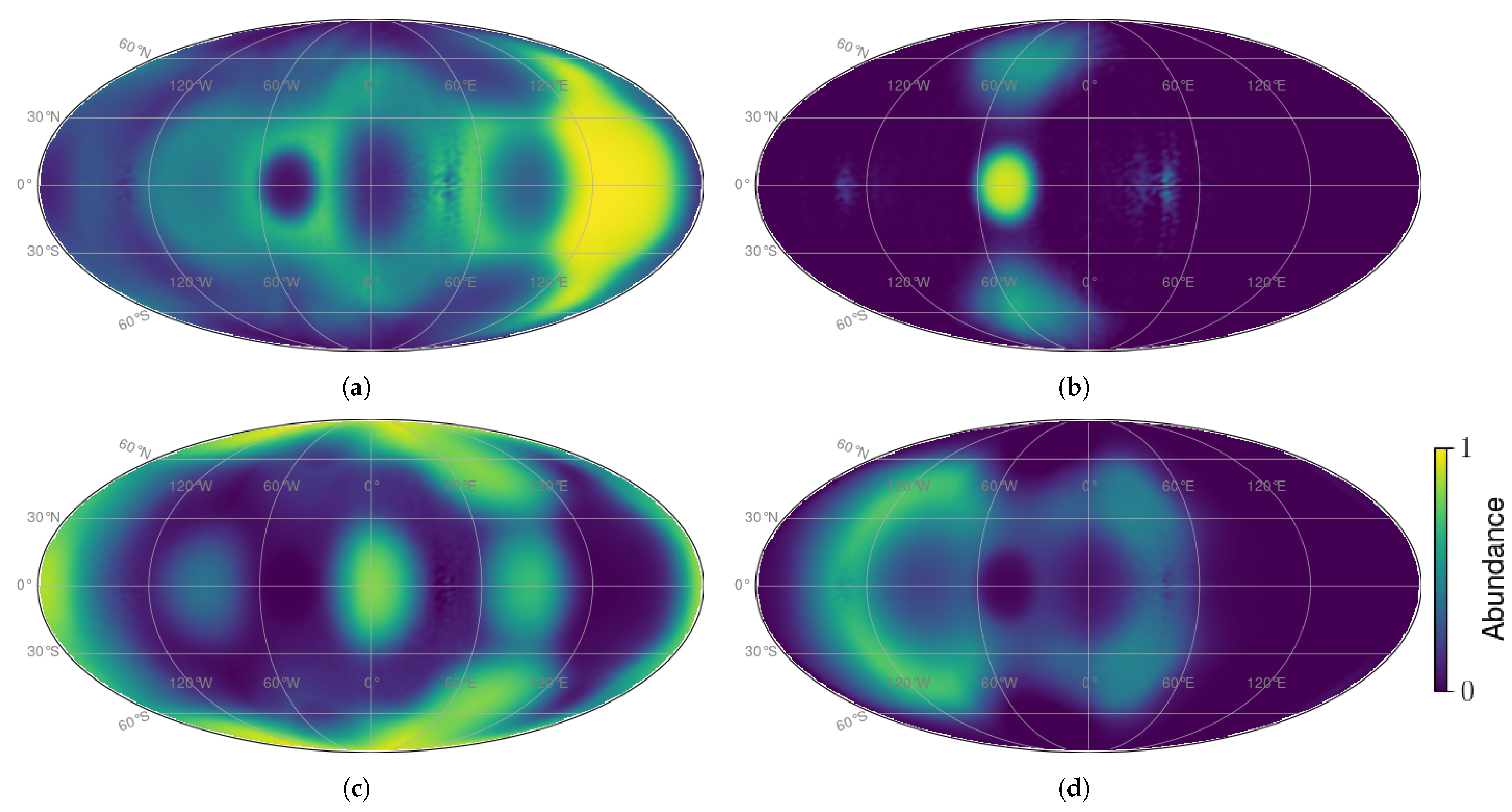
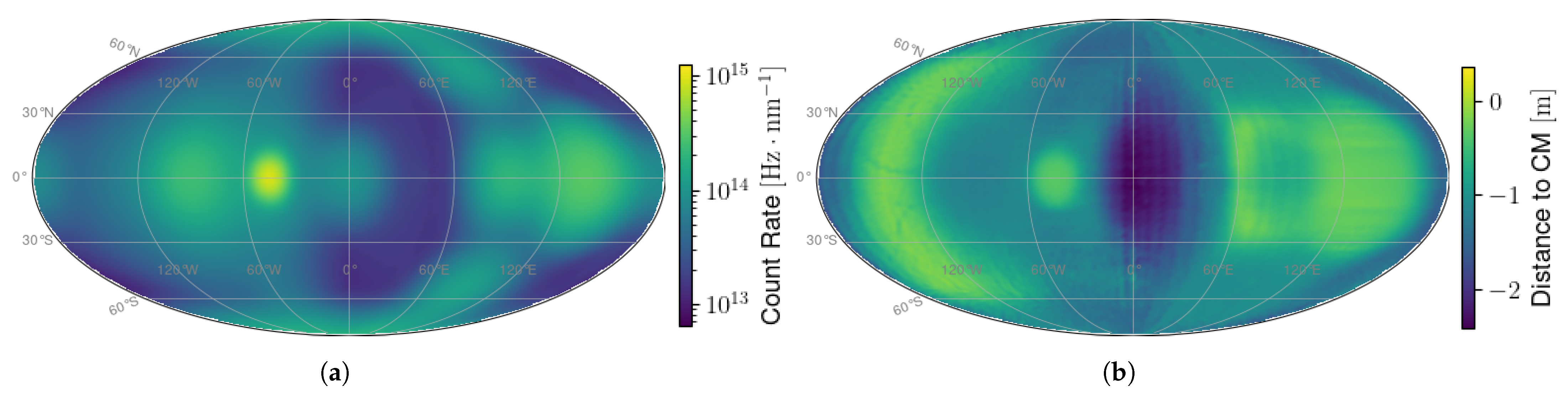
To demonstrate the potential of this projection technique, backscattering simulations of the box-wing satellite from Figure 4 were performed under solar illumination. Figure 16 shows the derived reflection and mean ranging estimate distributions for a single observation band. Given reflection distributions across multiple observation bands, the previously introduced spectral unmixing methods can be applied to determine material contribution maps for the target; see Figure 17. The resulting visualisations allow for better characterisation and differentiation between targets.

This approach provides the basis for determining the attitude and rotation parameters of a given pass. Assuming that the target rotates around a single body axis, which is known from its inertia tensor, then the corresponding rotation period can be calculated using commonly employed frequency analysis algorithms such as Least Squares Spectral Analysis (LSSA). Thus, only the orientation of the body frame with respect to the inertial frame remains unknown.

A grid search over possible Right Ascension (RA) and Declination (Dec) of the target’s rotation axis in Geocentric Celestial Reference System (GCRS) coordinates can be conducted. At each point in the grid, a new trajectory is determined from the initial rotation matrix of the target, which in turn is used to generate a synthetic light curve and evaluate its least squares error to the reference light curve.

To reduce computational effort, a full spectral reflectivity map, consisting of 10,000 evenly distributed phase vectors, was computed in under 48 h on an Nvidia GeForce RTX 2080Ti graphics card. The brightness associated with any particular viewing direction can be estimated by interpolating between the pre-calculated points on the reflectivity map. This approach is computationally more efficient than rendering each light curve in the search sequentially, as similar phase angles would be rendered repeatedly over the course of the full optimisation.

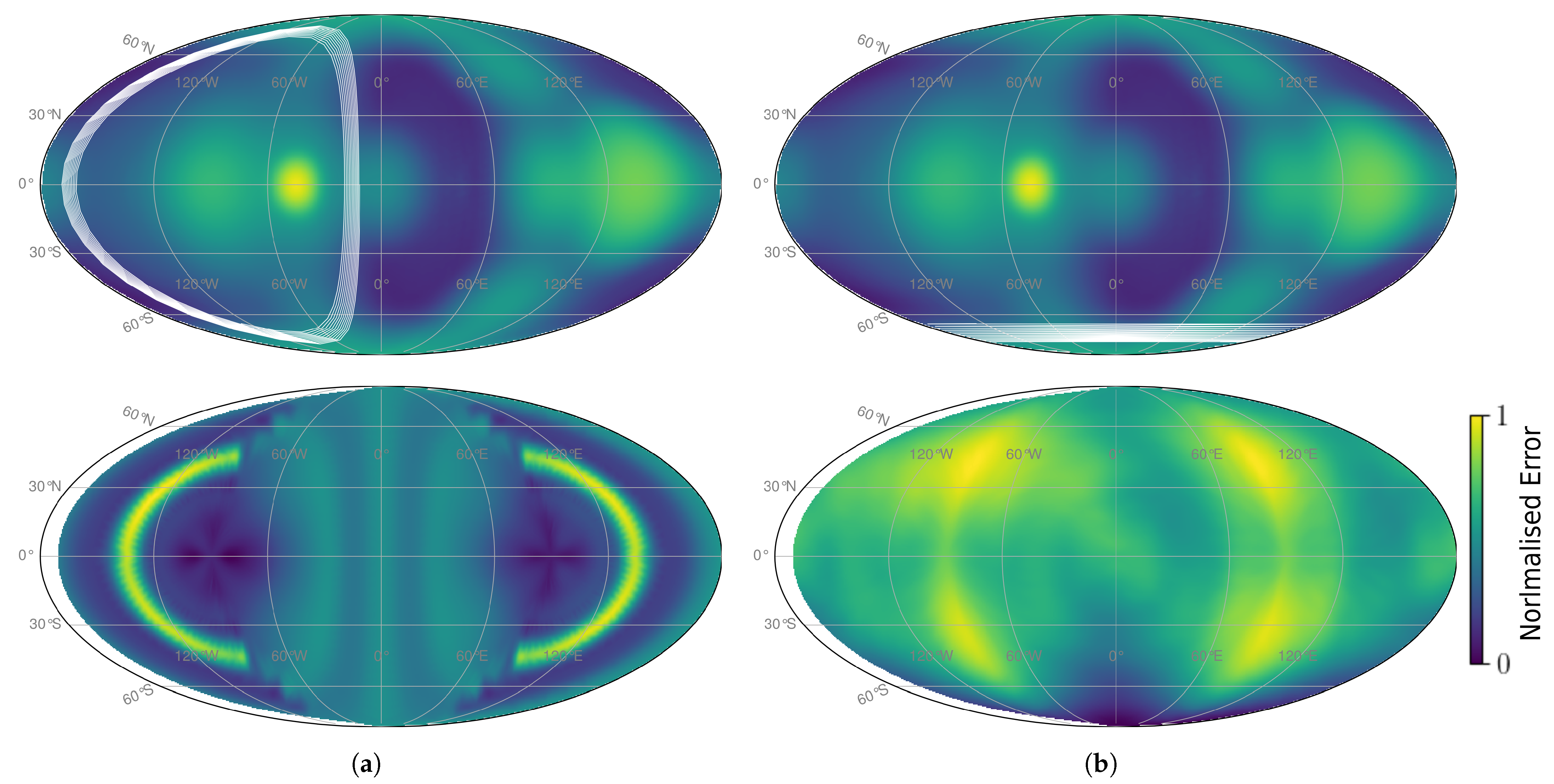
Conditioning of estimates is improved by carrying out interpolation across reflectivity and ranging maps for all bands as well as the material contribution maps. Figure 18 shows the mean of least squares errors of the interpolated count rates, ranging returns and material contributions. To avoid any bias, count rate and ranging distributions are normalised beforehand. The true trajectory of observation directions is represented as a white line in the body frame. For visualisation purposes, these plots show a cross section of the error surface, where the phase of the rotation around the rotation axis is fixed at the start epoch of the simulation.

Considering Figure 18, it is apparent that the error surfaces are not convex and have multiple local minima. Ergo, attempts to determine the true target attitude through least squares optimisation were only found to be successful as long as the initial guess was in close proximity to the correct parameters. Despite this, an optimum point on the error grid is apparent in both cases. The second minimum around the inverse rotation axis in Figure 18a is a result of the targets symmetry with respect to its equatorial plane. Cross-shaped fluctuations around the minima are features of the interpolation between grid points in the plot.

6. Conclusions

A spectral light curve simulator was developed to reproduce ground-based observations from space debris. The application provides options to model active and passive light curve observations, as well as predict return rates and centre of mass range offsets from laser ranging measurements to non-cooperative targets. By including open-source software such as the Mitsuba2 render engine and the atmospheric transfer library libRAdTran, the simulation pipeline is optimised. Spacecraft materials are specified via the interface of the render engine through BRDF measurements using an adaptive sampling technique or parametrised BRDF models. The validity of the simulation environment was verified through a quantitative comparison to field measurements of radar calibration spheres. Although these simple calibration targets do not capture the full capability of the software, they were selected due to the restricted availability of shape, surface material and attitude information for satellites. To attain a validation based on more complex targets, a cooperation with a satellite manufacturer and operator is envisioned for future studies.

The simulation toolkit was equipped with algorithms to demonstrate the potential of synthetic products for studies on parameter estimation from spacecraft. Thereby, material properties as well as rotation and attitude parameters were determined for a box-wing satellite using a limited set of prior knowledge. Much research is still to be conducted before these methods can be exploited to reliably extract attributes from space debris. However, the presented methods yield promising approaches to achieve this.

As the current ranging estimate does not consider multi-bounce reflections, one area of future development will be the Monte Carlo integration of the path length of rays to allow for more accurate ranging predictions. Moreover, simulations may be extended to include polarised light and resolved imaging to make use of all available information from measurements. The latter is especially relevant when considering the large increase of objects in LEO in recent years and the amount of satellites that are yet to be launched [1], for which moderately resolved imaging may hold valuable status information.

Further potential for research is provided by the differentiable rendering capabilities of Mitsuba2. Exploiting derivatives may help increase the efficiency of attribute estimations.