Identification of Time Variations of Moving Loads Applied to Plates Resting on Viscoelastic Foundation Using a Meshfree Method

Abstract

Dynamic identification of the intensity of the moving loads applied to structures is an important task in aerospace, marine, and transportation industries. In the present work, a general technique is presented for identification of the time variations in moving loads applied to plate structures resting on viscoelastic foundation. The identification problem is formulated as an inverse problem, which utilizes dynamic responses. The direct analyses required for the identification problem are performed by a meshfree method based on the moving node technique. In this technique, a node, which travels with the applied force, is utilized in the meshfree method. Since there is no connectivity between the nodes of meshfree methods, this technique can be implemented easily, while reducing the computational labor. Another benefit of this technique is that any simple or complicated trajectory of the moving load can be handled without any additional concerns. Two numerical example problems are solved and the effects of several parameters, including the measurement error, and number of sensors on the accuracy of the results are investigated. Through the examples, it is shown that the presented technique can identify the time variations in moving loads efficiently and accurately.

1. Introduction

The need for modeling and analysis of structures with special conditions is increasing in many engineering fields. Analysis of beams and plates resting on an elastic or viscoelastic foundation has many important applications in mechanical and aerospace engineering [1]. While direct analysis of plates under different conditions is still an active area of research [2,3,4], inverse analysis of plates for identification of applied loads has attracted the attention of many researchers [5,6,7]. Identification of a moving load can be carried out by a suitable inverse analysis and using measurement of dynamic structural responses such as displacement, velocity, or acceleration at some sampling points.

Direct analysis of plates subjected to moving loads has been performed by many investigators. Some of these works are reviewed here. Wu et al. [8] presented a finite element method (FEM) for analysis of dynamic behavior of simple plates under moving loads. They used the Newmark integration method and considered a fixed mesh in the finite element modeling of the problem. Zaman et al. [9] presented an FEM with a fixed mesh to determine the dynamic behaviors of thick plates resting on viscoelastic foundation subjected to moving point loads. They conducted a parametric study to determine the effects of different parameters on the response of the plate. The dynamic response of plates subjected to moving concentrated masses is different from the dynamic behavior of plates under moving point loads. Gbadeyan and Oni [10] developed an analytical method for determining the structural response of a rectangular plate subjected to concentrated moving masses. They assumed simply supported edges for the plate and used a double Fourier finite integral transformation method for solving the problem. Kim and Roesset [11] developed three analytical methods for determining dynamic responses of an infinite plate on elastic foundation under a moving load. They considered a moving load of constant magnitude and a moving harmonic load.

Malekzadeh et al. [12] presented a method based on the three-dimensional elasticity theory for determining the dynamic behavior of simply supported cross-ply laminated plates under moving point loads. They employed the layerwise theory, the modal analysis, and the differential quadrature method in their formulation. Cao et al. [13] employed the moving element method (MEM) for the dynamic analysis of composite plates resting on a Pasternak foundation under a moving load. The MEM is based on the FEM and is formulated in a coordinates system moving with the load. Praharaj and Datta [14], using a semi-analytical method, investigated the structural response of rectangular plates on viscoelastic foundation under a moving point load. They performed a parametric study to determine the effects of the viscoelastic foundation, velocity, and acceleration of the moving load on the dynamic response of the plate.

Moving load identification is an active research area, which has received considerable attention. Many studies have been performed on the identification of moving loads on beams, e.g., Refs. [15,16,17]; however, investigations on the identification of moving loads on plates are very limited. The problem of load identification is an inverse problem, which may be an ill-posed problem. Inverse problems are usually much more difficult than direct problems and require special treatments [18,19,20].

Zhu and Law [21] presented a method based on the modal superposition principle for identification of moving loads on a rectangular orthotropic plate. They employed the Tikhonov regularization method to obtain more stable solutions. They observed that acceleration responses gave better results than strain data. Law et al. [22] numerically and experimentally investigated the problem of moving load identification on a rectangular plate. They formulated the equation of motion in state space and employed the dynamic programming method for solving the inverse problem. They also presented a method for optimal selection of the magnitude of the regularization parameter. Zhang et al. [23] developed a method similar to that by Law et al. [22] for identification of two loads moving in opposite directions on a rectangular orthotropic plate. They also investigated the effects of measurement errors and the eccentricity of the moving loads on the accuracy of the results. It is worth mentioning that the moving load path is assumed to be straight in the previous research [21,22,23].

This article concerns the identification of moving loads subjected to plates resting on viscoelastic foundation. The time-dependent variation in the magnitude of the moving load is computed using measured velocities at several sampling points. In order to be able to analyze general problems with arbitrary geometry of the plate, and arbitrary path of the moving load, a suitable numerical method must be employed for the direct analyses. We use the meshfree radial point interpolation method (RPIM) [24] for direct and sensitivity analyses. The reason for the selection of this method is that its shape functions possess the Kronecker delta function property, which leads to easy implementation of the essential boundary conditions, as well as, its low sensitivity to arrangement of the nodal points. The mesh generation stage, which is necessary in the FEM, is eliminated in the meshfree method. In the proposed meshfree technique, a node, which moves with the applied moving load, is considered. Since there is no connectivity between the nodes of the meshfree method, this moving node technique can be implemented easily. A gradient based optimization method and the Tikhonov regularization method are used for the inverse analysis. By presenting two numerical examples, the accuracy of the method and the effects of important parameters on the obtained solutions are investigated.

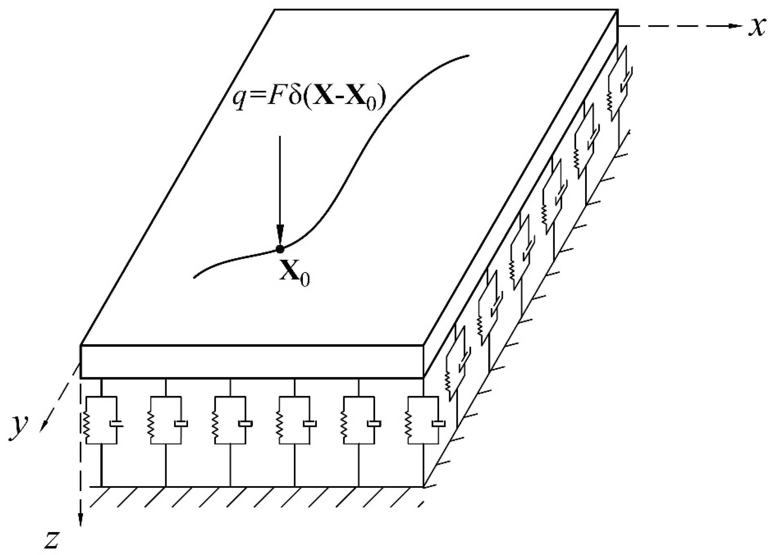
2. Meshfree Formulation of a Plate Resting on Viscoelastic Foundation under a Moving Load

There are several theories for defining the kinematics of plates subjected to lateral loading [3,25,26]. These theories can be divided into two main categories, i.e., theories for analysis of thin and moderately thick plates. One of the most useful and accurate plate theories, which can be used for a wide range of plate thicknesses, is the third order shear deformation theory (TSDT) [27]. In this theory, which is adopted in the present work, the displacement filed of a plate is written as follows [28]:

$$\widehat{u}=\left\{\begin{array}{c}u\\ v\\ w\end{array}\right\}=\left[\begin{array}{ccc}-\alpha z^3\frac{\partial }{\partial x}& z-\alpha z^3& 0\\ -\alpha z^3\frac{\partial }{\partial y}& 0& z-\alpha z^3\\ 1& 0& 0\end{array}\right]\left\{\begin{array}{c}w\\ {\varphi }_x\\ {\varphi }_y\end{array}\right\}=L_{u}u$$

(1)

In Equation (1), $\alpha =4/3h^2$ where h is the plate’s thickness, w is the lateral deflection, and ${\varphi }_x$ and ${\varphi }_y$ are the rotation of the normal to the cross section about y and x axes, respectively. For the TSDT, the linear strain field is given by:

$$\left\{\begin{array}{c}{\epsilon }_{xx}\\ {\epsilon }_{yy}\\ {\epsilon }_{xy}\\ {\epsilon }_{xz}\\ {\epsilon }_{yz}\end{array}\right\}=\left[\begin{array}{ccc}-\alpha z^3\frac{{\partial }^2}{\partial x^2}& \left(z-\alpha z^3\right)\frac{\partial }{\partial x}& 0\\ -\alpha z^3\frac{{\partial }^2}{\partial y^2}& 0& \left(z-\alpha z^3\right)\frac{\partial }{\partial y}\\ -2\alpha z^3\frac{{\partial }^2}{\partial x\partial y}& \left(z-\alpha z^3\right)\frac{\partial }{\partial y}& \left(z-\alpha z^3\right)\frac{\partial }{\partial x}\\ \left(1-3\alpha z^2\right)\frac{\partial }{\partial x}& \left(1-3\alpha z^2\right)& 0\\ \left(1-3\alpha z^2\right)\frac{\partial }{\partial y}& 0& \left(1-3\alpha z^2\right)\end{array}\right]\left\{\begin{array}{c}w\\ {\varphi }_x\\ {\varphi }_y\end{array}\right\}=Lu$$

(2)

For a plate made of an isotropic linear elastic material, the following constitutive relation between the stress and strain fields holds:

$$\left\{\begin{array}{c}{\sigma }_{xx}\\ {\sigma }_{yy}\\ {\sigma }_{xy}\\ {\sigma }_{xz}\\ {\sigma }_{yz}\end{array}\right\}=\frac{E}{1-{\upsilon }^2}\left[\begin{array}{ccccc}1& \upsilon & 0& 0& 0\\ \upsilon & 1& 0& 0& 0\\ 0& 0& \left(1-\upsilon \right)/2& 0& 0\\ 0& 0& 0& \left(1-\upsilon \right)/2& 0\\ 0& 0& 0& 0& \left(1-\upsilon \right)/2\end{array}\right]\left\{\begin{array}{c}{\epsilon }_{xx}\\ {\epsilon }_{yy}\\ {\epsilon }_{xy}\\ {\epsilon }_{xz}\\ {\epsilon }_{yz}\end{array}\right\}=D\mathsf{\epsilon }$$

(3)

where E and $\upsilon$ are the Young’s modulus and Poisson’s ratio of the material, respectively.

In solid mechanics problems, energy principles are widely used for derivation of the governing equations. Furthermore, the discretized form of the governing equations can be obtained by means of the energy principles. Hamilton’s principle is the energy method used for analysis of the dynamical systems [29,30]. For a plate resting on a viscoelastic foundation, as shown in Figure 1, the equation of motion can be obtained based on the Hamilton’s principle, i.e.,:

$$\delta {\displaystyle {\int }_{t_1}^{t_2}\left[K-\left(V+U\right)\right]dt}=0$$

(4)

where K, U, and V are the kinetic energy, strain energy, and the work conducted by the external loads, respectively. The variation in these quantities for the plate of Figure 1 is defined as:

$$\delta K={\displaystyle {\int }_{\mathsf{\Omega }}\rho \left[\delta {(L_u\dot{u})}^T{L}_u\dot{u}\right]d\mathsf{\Omega }},$$

(5)

$$\delta U={\displaystyle {\int }_{\mathsf{\Omega }}\left(\delta {\mathsf{\epsilon }}^T\mathsf{\sigma }\right)d\mathsf{\Omega }}={\displaystyle {\int }_{\mathsf{\Omega }}\left(\delta {\mathsf{\epsilon }}^{T}D\mathsf{\epsilon }\right)d\mathsf{\Omega }},$$

(6)

$$\delta V=-{\displaystyle {\int }_{\mathsf{\Omega }}\left[\delta w\left(q-k_{f}w-c_f\dot{w}\right)\right]d\mathsf{\Omega }},$$

(7)

where $k_f$ and $c_f$ are the stiffness and damping coefficients of the foundation, and q is the lateral distributed load. Upon substitution of Equations (5)–(7) into Equation (4), and performing necessary integration by parts on the time variable, the Hamilton’s principle can be written as:

$${\displaystyle {\int }_{\mathsf{\Omega }}\rho \left[\delta {(L_{u}u)}^T{L}_u\ddot{u}\right]d\mathsf{\Omega }}+{\displaystyle {\int }_{\mathsf{\Omega }}\left(\delta {\mathsf{\epsilon }}^{T}D\mathsf{\epsilon }\right)d\mathsf{\Omega }}+{\displaystyle {\int }_{\mathsf{\Omega }}\left[\delta w\left(k_{f}w+c_f\dot{w}\right)\right]d\mathsf{\Omega }}={\displaystyle {\int }_{\mathsf{\Omega }}\delta wqd\mathsf{\Omega }}.$$

(8)

Now the displacement field of the plate, i.e., u, should be approximated by a proper meshfree technique. In the present work, the meshfree RPIM is used for construction of the approximate displacement field, as follows:

$$u={\displaystyle \sum _{J=1}^n\left[\begin{array}{ccc}{\phi }_J& 0& 0\\ 0& {{\phi }^{\prime }}_J& 0\\ 0& 0& {{\phi }^{\prime }}_J\end{array}\right]\left\{\begin{array}{c}{w}_J\\ {\varphi }_{xJ}\\ {\varphi }_{yJ}\end{array}\right\}}={\displaystyle \sum _{J=1}^n{\mathsf{\psi }}_J{u}_J},$$

(9)

where ${\phi }_J$ and ${{\phi }^{\prime }}_J$ are the RPIM shape functions used for interpolation of the lateral deflection and rotation, respectively. These shape functions can be of the same or different orders. Details on construction of the RPIM shape functions can be found in [3,26]. Upon substitution of Equation (9) into Equation (2), the approximated strain field is obtained. Subsequently, by substituting the strain field into Equation (3), the approximated stress field will also be obtained as follows:

$$\mathsf{\epsilon }={\displaystyle \sum _{J=1}^n\left(L{\mathsf{\psi }}_J\right)u_J={\displaystyle \sum _{J=1}^n{B}_J{u}_J}},$$

(10)

$$\mathsf{\sigma }={\displaystyle \sum _{J=1}^{n}D{B}_J{u}_J}.$$

(11)

Finally, the approximate fields of the meshfree RPIM can be substituted into the Hamilton’s principle, Equation (8), to give the following system of discretized equations:

$$\left[M\right]\left\{\ddot{d}\right\}+\left[C\right]\left\{\dot{d}\right\}+\left[K\right]\left\{d\right\}=\left\{F\right\},$$

(12)

where the components of the mass, damping, and stiffness matrices, and the load vector can be written as:

$$M_{IJ}={\displaystyle {\int }_{\mathsf{\Omega }}\rho {\left(L_u{\mathsf{\psi }}_I\right)}^T}\left(L_u{\mathsf{\psi }}_J\right)d\mathsf{\Omega }={\displaystyle {\int }_{\mathsf{\Omega }}\rho B_{uI}{}^T{B}_{uJ}d\mathsf{\Omega }},$$

(13)

$$C_{IJ}={\displaystyle {\int }_{\mathsf{\Omega }}{c}_f{N}_{wI}^T{N}_{wJ}d\mathsf{\Omega }},$$

(14)

$$K_{IJ}={\displaystyle {\int }_{\mathsf{\Omega }}{B}_I^{T}D{B}_J^{T}d\mathsf{\Omega }}+{\displaystyle {\int }_{\mathsf{\Omega }}{k}_f{N}_{wI}^T{N}_{wJ}d\mathsf{\Omega }},$$

(15)

$$F_I={\displaystyle {\int }_{\mathsf{\Omega }}q{N}_{wI}d\mathsf{\Omega }},$$

(16)

where $N_{\mathrm{w}I}$ is the matrix of shape functions associated with the lateral deflection, i.e.,:

$$N_{\mathrm{w}I}=\left[\begin{array}{ccc}{\phi }_I& 0& 0\\ 0& 0& 0\\ 0& 0& 0\end{array}\right]$$

(17)

The system of ordinary differential Equation (12) can be solved using the standard time marching schemes, such as the Newmark’s method.

In the present study, it is assumed that the plate is subjected to a moving concentrated load. For the numerical analysis of the plate it is ideal to have a node at the point of application of the force. Since the moving force might travel on any arbitrary path, in this study, a moving node which travels with the force is added to the nodal arrangement of the plate. By this strategy it is guaranteed that at any time step, there is a node at the point of application of the moving force. It should be mentioned that this strategy can only be implemented in meshfree methods, where there is no connectivity between the nodal points, and therefore, any nodal point can freely move during the problem analysis.

3. Inverse Analysis

This study considers a plate with an arbitrary geometry and known boundary conditions resting on viscoplastic foundation with known parameters. A moving load with a known path is applied to the plate. The aim of the inverse problem is to find the unknown time-dependent magnitude of the moving load using measured velocities at several points on the plate. In inverse problems, in order to obtain the unknowns, an optimization problem is defined. The goal of the optimization is to find the values of the unknowns, such that the difference between values of a measured quantity and those obtained from the inverse analysis becomes a minimum.

The total time interval of the problem is divided into $n$ equal time intervals (steps). Several sampling points with fixed locations are considered for velocity measurement. The vector of measured velocities at time $t_i$ is expressed as:

$$Y^{(t_i)}={\left[\begin{array}{cccc}{Y}_1^{(t_i)}& Y_2^{(t_i)}& \cdots & Y_{N_S}^{(t_i)}\end{array}\right]}^{\mathrm{T}},$$

(18)

where $N_S$ represents the number of sampling points.

We need to solve many direct problems in the inverse analysis. The velocity computed by a direct analysis at the sampling point $j$ at time $t_i$, is represented by $v_j^{(t_i)}$. The vector of computed velocities at the sampling points at time $t_i$ is expressed as follows:

$$v^{(t_i)}={\left[\begin{array}{cccc}{v}_1^{(t_i)}& v_2^{(t_i)}& \cdots & v_{N_S}^{(t_i)}\end{array}\right]}^{\mathrm{T}},$$

(19)

Considering all time steps, the global vector of measured velocities can be expressed as follows:

$$Y=\left[\begin{array}{c}{Y}^{(t_1)}\\ \begin{array}{l}{Y}^{(t_2)}\\ ⋮\end{array}\\ Y^{(t_n)}\end{array}\right].$$

(20)

Similarly, the global vector of computed velocities at sampling points can be expressed as follows:

$$v(X)=\left[\begin{array}{c}{v}^{(t_1)}(X)\\ \begin{array}{l}{v}^{(t_2)}(X)\\ ⋮\end{array}\\ v^{(t_n)}(X)\end{array}\right].$$

(21)

where $X$ is the global vector of unknowns, which contains the magnitude of the moving load at all time steps and is expressed as follows:

$$X={\left[\begin{array}{cccc}{q}_1& q_2& \cdots & q_n\end{array}\right]}^{\mathrm{T}}.$$

(22)

In Equation (22), $q_i=q(t_i)$ represents the magnitude of the moving load at time $t_i$. In the inverse analysis, we have to find the vector of unknowns such that the computed velocities become as close as possible to the measured velocities. For this purpose a cost function is defined as follows:

$$f(X)={[Y-v(X)]}^{\mathrm{T}}[Y-v(X)].$$

(23)

Due to the ill-posed nature of the inverse problem, the solution obtained from minimization of the objective function in Equation (23) may be oscillatory and therefore, a suitable regularization method should be employed. In this work, the Tikhonov regularization (TR) method [31] is used. Based on the TR method, the objective function in Equation (23) is modified as follows:

$$\begin{array}{c}f(X)={[Y-v(X)]}^{\mathrm{T}}[Y-v(X)]+{\gamma }_0{(H_{0}X)}^T(H_{0}X)+\\ {\gamma }_1{(H_{1}X)}^T(H_{1}X)+{\gamma }_2{(H_{2}X)}^T(H_{2}X) ,\end{array}$$

(24)

where the terms with the regularization parameters ${\gamma }_0$, ${\gamma }_1$, and ${\gamma }_2$ are, respectively, zeroth, first and second order TR terms. $H_o, H_1$ and $H_2$ are $n\times n$ matrices and are expressed as follows:

$$H_0=\left[\begin{array}{cccc}1& 0& \cdots & 0\\ 0& 1& \ddots & ⋮\\ ⋮& \ddots & \ddots & 0\\ 0& \cdots & 0& 1\end{array}\right] ,$$

(25)

$$H_1=\left[\begin{array}{cccccc}-1& 1& 0& \cdots & 0& 0\\ 0& -1& 1& \cdots & 0& 0\\ ⋮& ⋮& ⋮& ⋮& ⋮& ⋮\\ 0& 0& \cdots & -1& 1& 0\\ 0& 0& \cdots & 0& -1& 1\\ 0& 0& 0& 0& 0& 0\end{array}\right] ,$$

(26)

$$H_2=\left[\begin{array}{ccccccccc}1& -2& 1& 0& \cdots & 0& 0& 0& 0\\ 0& 1& -2& 1& \cdots & 0& 0& 0& 0\\ ⋮& ⋮& ⋮& ⋮& ⋮& ⋮& ⋮& ⋮& ⋮\\ 0& 0& 0& 0& \cdots & 1& -2& 1& 0\\ 0& 0& 0& 0& \cdots & 0& 1& -2& 1\\ 0& 0& 0& 0& 0& 0& 0& 0& 0\\ 0& 0& 0& 0& 0& 0& 0& 0& 0\end{array}\right] .$$

(27)

Selecting suitable values for ${\gamma }_0$, ${\gamma }_1$, and ${\gamma }_2$ results in accurate and stable solutions. It has been observed that the second order TR term is more effective than the other ones and it can sufficiently reduce the oscillations in the solutions of the inverse problem [32]. Therefore, only the second order TR term is considered and the objective function is rewritten as follows:

$$f(X)={[Y-v(X)]}^{\mathrm{T}}[Y-v(X)]+\gamma {(H_{2}X)}^T(H_{2}X) .$$

(28)

Some different methods can be employed for the proper selection of the regularization parameter $\gamma$. The discrepancy principle [33] is used in this study. Based on this method, the regularization parameter is selected in a way that the difference between computed and measured velocities at the sampling points would become of the same order as the error of the measured velocities.

To minimize the objective function in Equation (28), its derivative with respect to the vector $X$ is set to zero:

$${\nabla }_{X}f={\nabla }_X\left\{ {[Y-v(X)]}^T[Y-v(X)]\right\}+\gamma {\nabla }_X[{(H_{2}X)}^T(H_{2}X)]=0.$$

(29)

Since the problem is linear, the vector $v(X)$ can be written as follows:

$$v(X)=SX.$$

(30)

where $S$ is the sensitivity matrix and can be written as follows:

$$S=\left[\begin{array}{cccc}{S}_{1,1}& 0& \cdots & 0\\ S_{2,1}& S_{2,2}& \cdots & 0\\ ⋮& ⋮& \ddots & ⋮\\ S_{n,1}& S_{n,1}& \cdots & S_{n,n}\end{array}\right].$$

(31)

Sub-matrices in Equation (31) are expressed as follows:

$$S_{i,j}=\left[\begin{array}{c}\frac{\partial v_1^{(t_i)}}{\partial q_j}\\ ⋮\\ \frac{\partial v_{N_S}^{(t_i)}}{\partial q_j}\end{array}\right].$$

(32)

Entries of $S_{i,j}$ represent the derivative of the velocities at the sampling points at the time step $i$, with respect to $q_j$. To find the sensitivity coefficients, we must solve $n$ direct problems. In the j-th direct problem, we apply a unit load at time $j$ (during a time step interval) at the location of $q_j$. Since the problem is linear, the solution of the direct problem for velocities at the sampling points, i.e., $v_1^{(t_i)}$, …, $v_{N_S}^{(t_i)}$, represent $\partial v_1^{(t_i)}/\partial q_j$, …, $\partial v_{N_S}^{(t_i)}/\partial q_j$, respectively. After computation of the sensitivity matrix, using Equations (29) and (30), the vector of unknowns can be obtained using the following equation:

$$X={(S^{T}S+\gamma H_2^T{H}_2)}^{-1}{S}^{T}Y.$$

(33)

4. Results and Discussion

In this section, two numerical example problems are provided to demonstrate the usefulness of the proposed identification technique. In the example problems, the time variation in moving loads applied to plates resting on viscoelastic foundation is identified. Effects of measurement error, number and position of sensors, and the regularization method are studied through the numerical examples. In the first example problem, the moving load’s path is a straight line, and therefore it is easy to place nodal points of the meshfree method on the load’s path. In the second example, it is assumed that the load travels on a curved path. As a result, a uniform nodal arrangement is used for modelling the plate, while an additional node is added to the nodal arrangement for easy application of the moving force. Since there is no connectivity between the nodes of meshfree methods, this additional node travels freely with the concentrated force and therefore the application of the moving force in the meshfree method is enhanced.

It should be mentioned that in the present work the experiments for the inverse analyses are simulated by direct analysis of the problem using the meshfree method. Firstly, a direct analysis with a known moving force is performed and the time variations in the velocity at some sampling points of the plate are recorded. Then, for simulation of the inherent measurement errors of the sensors in an actual experiment, some random errors with Gaussian distribution are added to the recorded values. These values are finally used as the inputs of the inverse algorithm and the time variations in the moving force are identified based on these recordings.

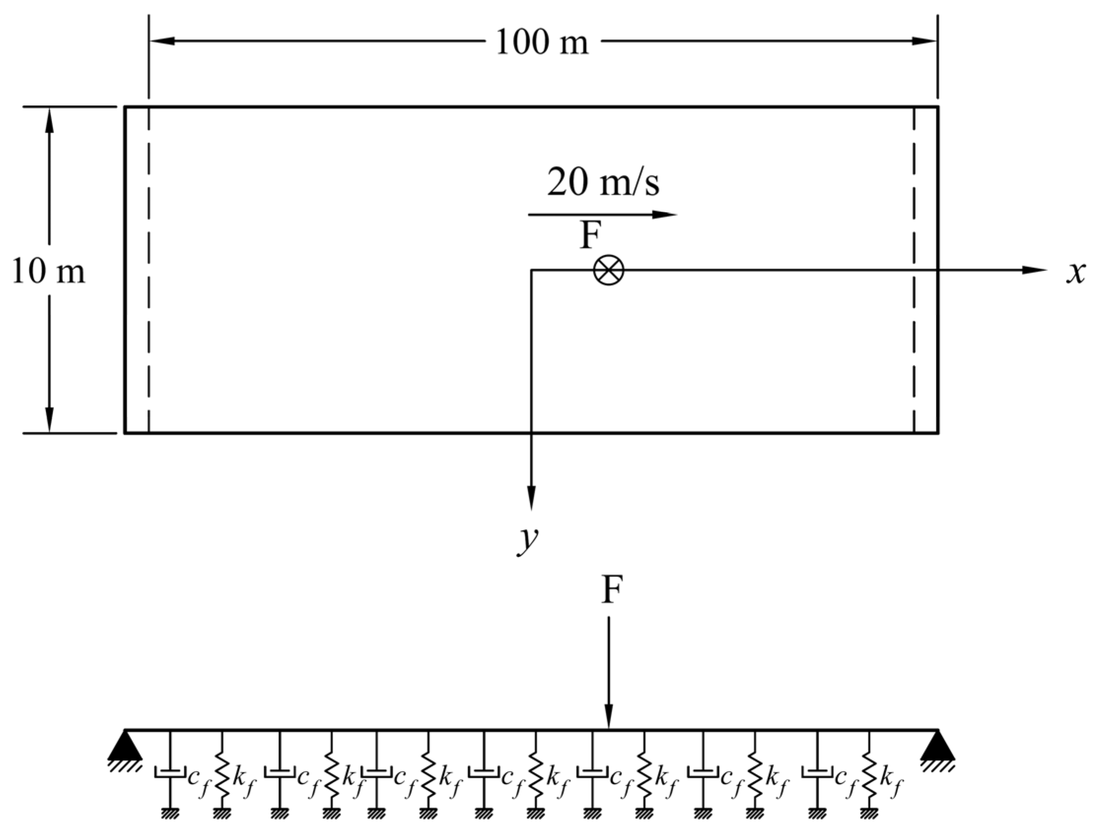
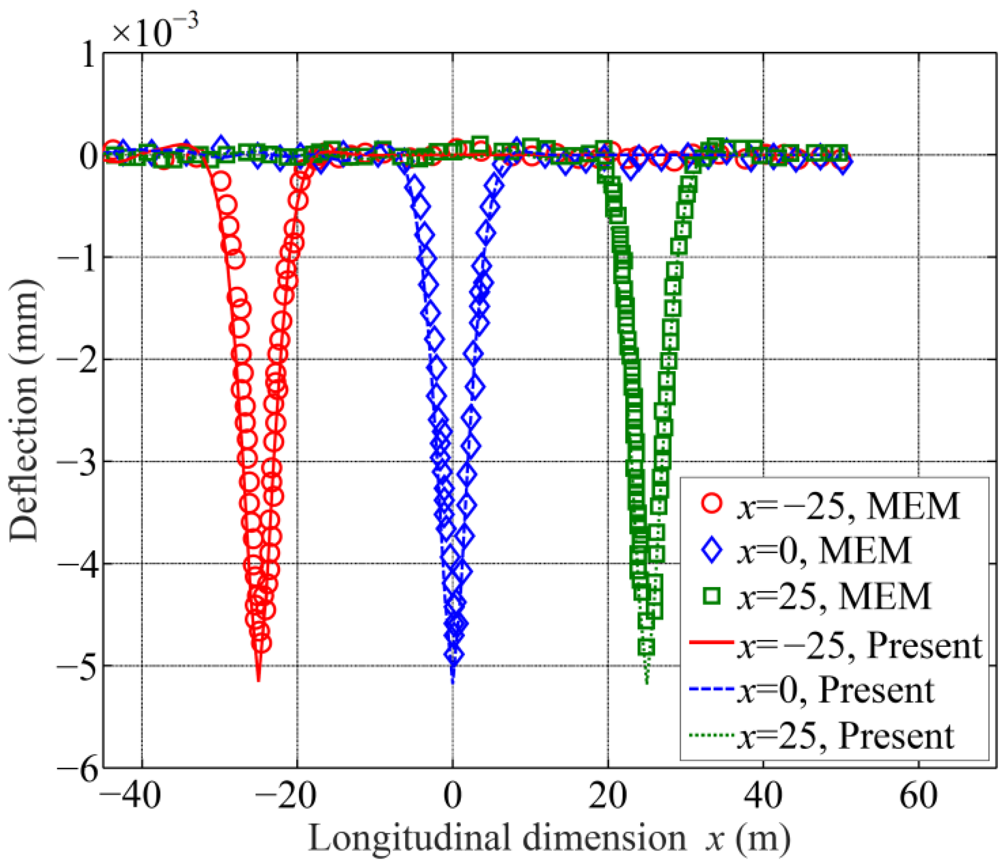
4.1. Verification of the Meshfree Method for Analysis of Moving Force Problems

Herein, a benchmark example problem is solved by the meshfree RPIM in order to assess the accuracy of the meshfree technique used in the inverse analyses of the present work. Figure 2 depicts the problem geometry, boundary, and loading conditions. A constant 1000 N moving force is applied to the longitudinal centerline of the plate. The force travels with a constant speed of 20 $\mathrm{m}/\mathrm{s}$. The material properties of the plate are as follows: $E=31 \mathrm{GPa},$$\upsilon =0.25,$ and $\rho =2440 \mathrm{kg}/{\mathrm{m}}^3.$ The plate’s thickness is 0.3 m and it is resting on an elastic foundation, with $k_f={10}^7 \mathrm{N}/{\mathrm{m}}^3.$ The results obtained by the meshfree RPIM are compared with those obtained by the moving element method (MEM) [34].

It should be mentioned that this problem was solved with three different nodal arrangements and convergence of the results was assessed accordingly. However, for the sake of conciseness, the results of all nodal arrangements are not reported herein. The reported results correspond to a uniform arrangement of 101 × 11 nodal points, and the time step size is $\Delta t=0.05 \mathrm{s}.$ Furthermore, the total number of integration points is 17,472. Figure 3 depicts the deflection of the plate along its longitudinal centerline at three different time instances. In this figure, results of the meshfree RPIM are compared with those of the MEM [34] and a close agreement is observed.

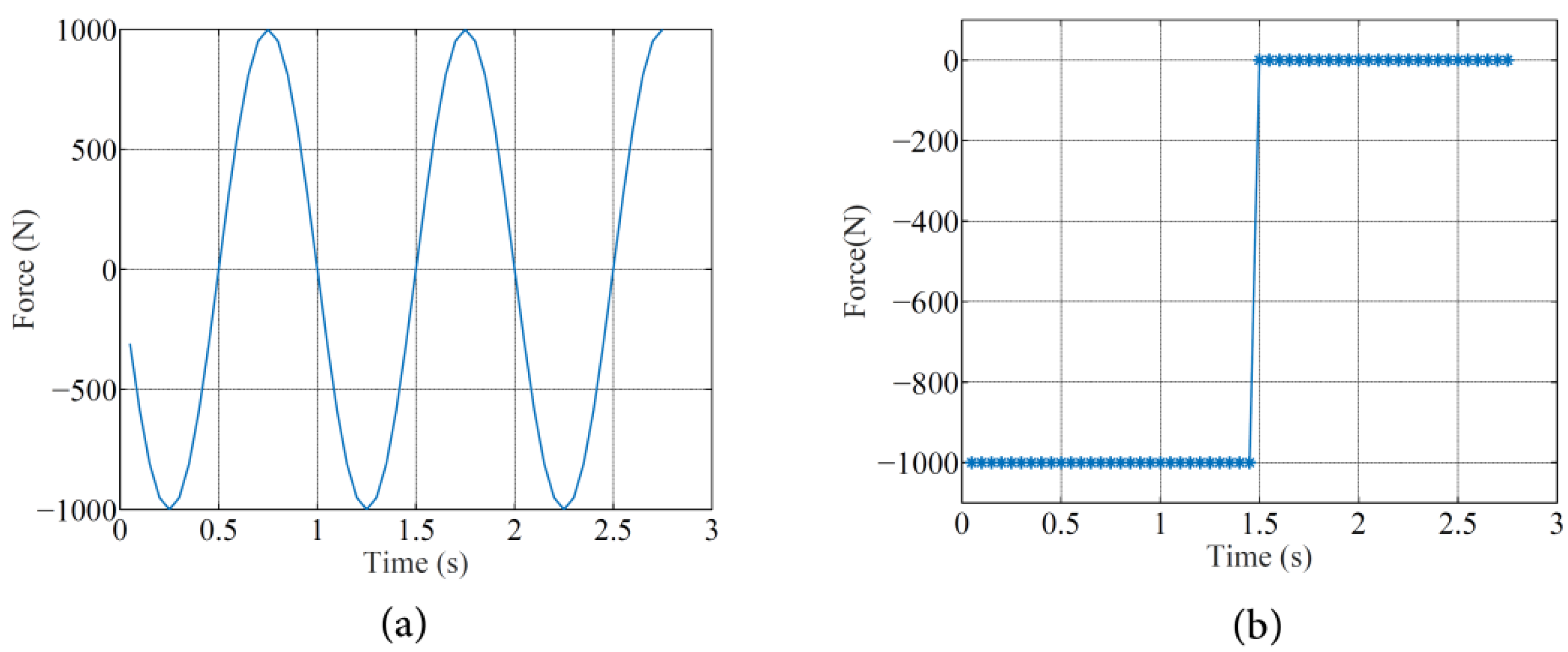
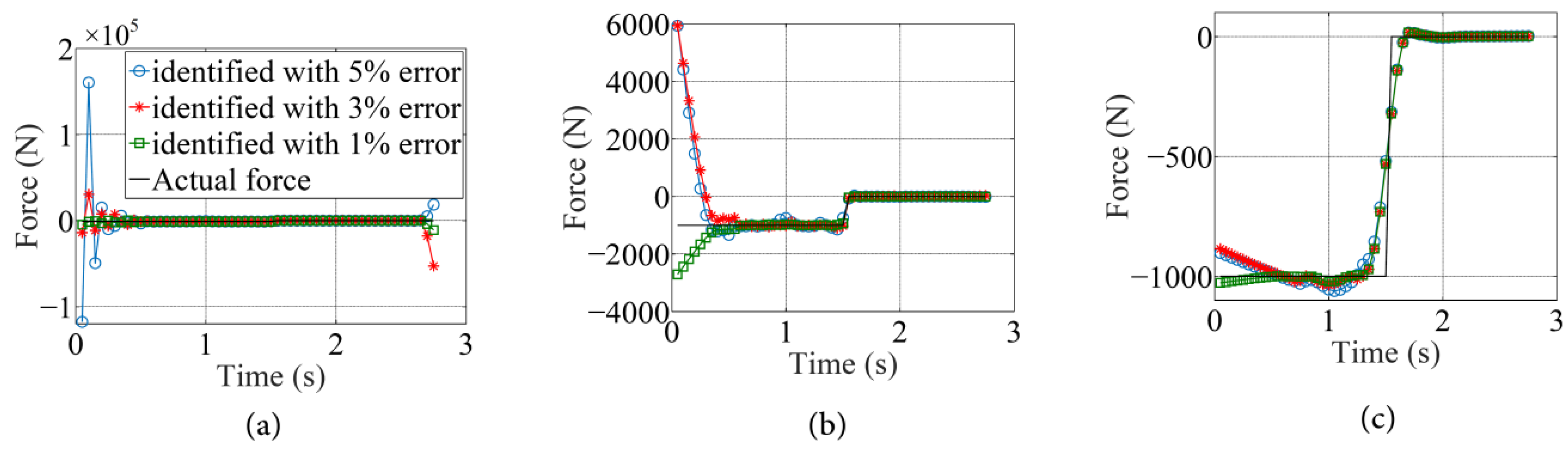
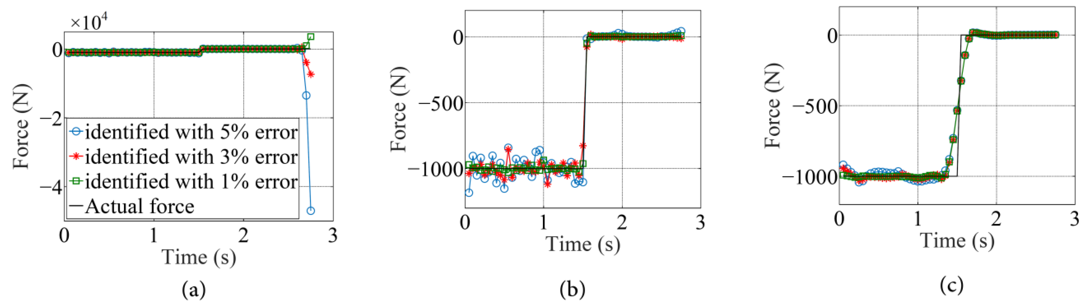
4.2. Example 1: Identification of Time Variation in a Moving Force Travelling on a Straight Path

In this example problem, the plate of the previous example is used for identification of the time variations in the applied moving force. The plate dimensions are $60 \mathrm{m}\times 10 \mathrm{m}$ and the force moves along the centerline of the plate, as shown in Figure 4. The positions of six velocity sensors are also shown in this figure.

Two different time variations in the moving load, i.e., sinusoidal and step function, are considered in this example. As mentioned previously, the values of the plate’s velocity at the sampling points are obtained for each time variation in the moving load, and are subsequently used as the inputs of the inverse algorithm. The two different time variations in the moving load are shown in Figure 5. Herein, a uniform arrangement of 61 × 11 nodal points and also a total of 13,440 integration points are used for the analyses.

The inverse identification problem is solved with different numbers of sensors, i.e., four, five, and six sensors. Furthermore, different levels of measurement error, i.e., 1%, 3%, and 5% are considered in the analyses. The identification results of these cases are then compared in order to assess the capability of the proposed technique for identification of a moving load in various conditions.

When there are no measurement errors, the identification of the moving load is achieved with only four sensors and no need of regularization. Figure 6a,b depict the identified time variations in the moving load for the sinusoidal and step function, respectively. It is seen that the actual and identified forces are almost the same.

Now the effect of measurement error and the number of sensors on the overall performance of the inverse algorithm is studied. Figure 7, Figure 8 and Figure 9 plot the time variation in the identified force with four, five, and six sensors respectively. In each figure, the effects of measurement error and the regularization technique are compared. Three different values for the regularization parameter, i.e., $\gamma =0,$ $\gamma ={10}^{-22},$ and $\gamma ={10}^{-18},$ are used in the analyses. These figures correspond to the sinusoidal loading.

Figure 7 demonstrates the importance of regularization when measurement errors are present in the identification process. It is also seen that when sensors one through four, which are placed inside the problem domain and far from the boundaries are used in the inverse analysis, the time variations in the moving load near the boundaries cannot be captured with an acceptable accuracy.

In an attempt to increase the accuracy of the identified force near the problem boundary, sensor 5 is also considered, and the inverse procedure is performed again. Figure 8 plots the identified time variations in the moving load for various values of the regularization parameter. It is seen that addition of a sensor, to the vicinity of the left boundary, has improved the identification accuracy at times when the moving load is close to this boundary.

Finally, the sixth sensor, which is located near the right boundary, is also considered in the inverse analysis. Figure 9 clearly shows how the addition of a sensor near the right boundary has improved the accuracy of the identification process at time instances when the moving force is near this boundary. It is also observed that when a sufficient number of sensors are used in the inverse analysis, the regularization process becomes less important. However, even in this case, the best results are obtained when a proper value of the regularization parameter is used. A comparison of Figure 8 and Figure 9 clearly demonstrates the effect of the number and position of the sensors on the accuracy of the identification process.

Now the identification problem is solved for the case of step function. The same number of sensors and the same levels of measurement error as the previous case are considered for the step function. The identified forces with four, five, and six sensors and different values of the regularization parameter are depicted in Figure 10, Figure 11, Figure 12 and Figure 13.

Figure 10 implies that, especially when a smaller number of sensors are used, the effect of regularization becomes more important. It is observed that without regularization, the identification process has failed, while proper value of the regularization parameter has led to acceptable results.

Figure 11 demonstrates that increasing the number of sensors to five, leads to improvement of the identification accuracy. Here again, the regularization process has successfully eliminated the unwanted oscillations of the solution. By increasing the number of sensors to six, the obtained results become more accurate, especially for the case with no regularization. Figure 12 shows that when sufficient number of sensors is used, the inverse algorithm can find the time variation in the moving load even with no regularization. However, even in this case, the best results are obtained when a proper value for the regularization parameter is selected.

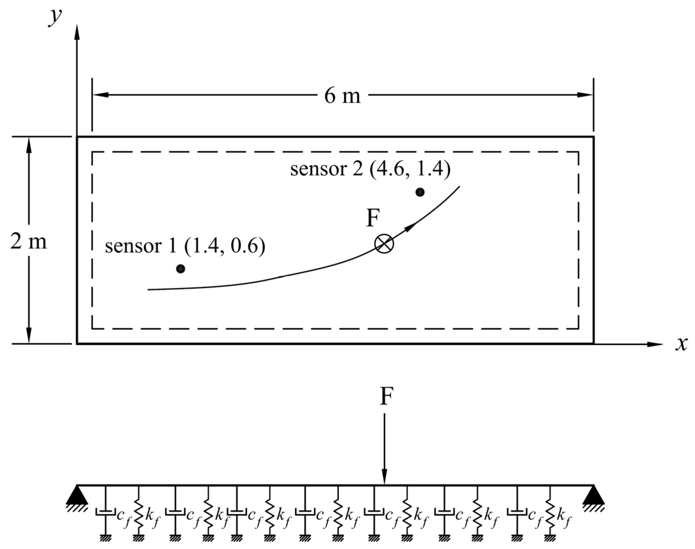
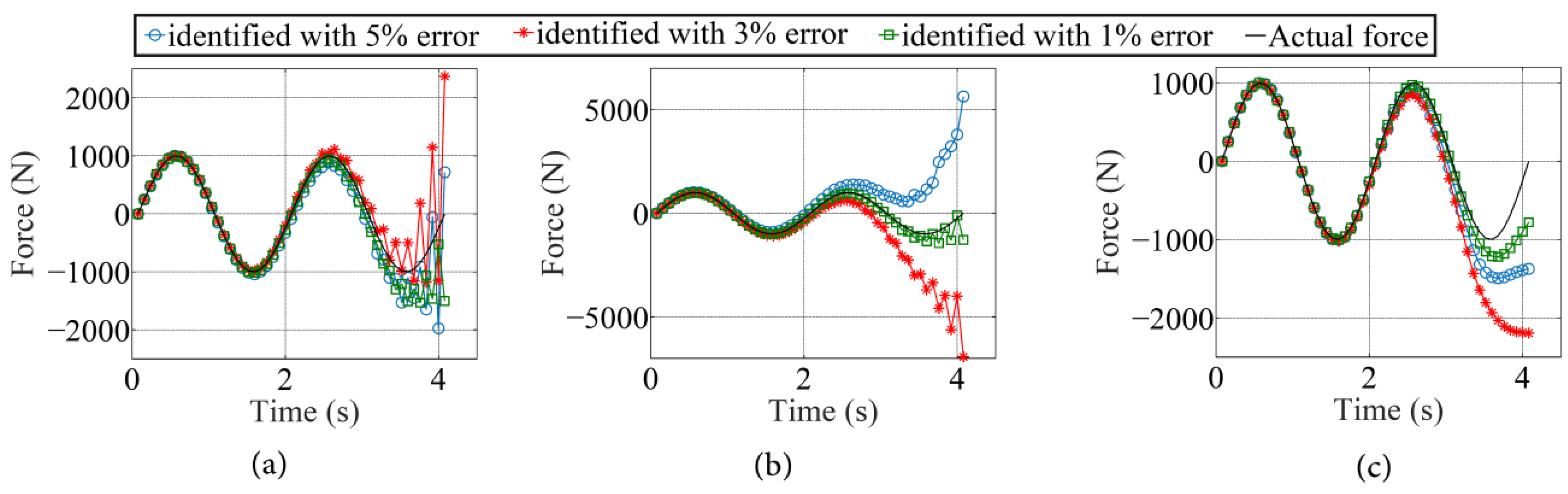
4.3. Example 2: Identification of Time Variation in a Moving Force Travelling on a Curved Path

In this example problem, it is assumed that the applied force moves along a curved path on a plate. The problem geometry, boundary, and loading conditions are depicted in Figure 13. The material properties of the plate and the constants of its viscoelastic foundation are the same as the previous example. The total number of nodes and integration points of this example problem are 392, and 9600, respectively. The parametric equation of the load’s path is as follows:

$$\{\begin{array}{l}x=t+1\\ y=0.075{\left(t+1\right)}^2-0.2\left(t+1\right)+0.625\end{array} 0\le t\le 4$$

(34)

In this example, two velocity sensors as depicted in Figure 13 are used for the inverse analyses. Similar to the previous example, the effects of measurement error, the number of sensors, and regularization technique on the accuracy of the identification process are studied. It is assumed that the actual load has a sinusoidal variation as shown in Figure 5a.

The inverse problem is firstly solved by considering the data obtained from sensor 1 alone. Figure 14 depicts the identified time variations in the moving load for various values of the regularization parameter, i.e.,$\gamma =0,$ $\gamma ={10}^{-22},$ and $\gamma ={10}^{-18}$. It is seen that proper selection of the regularization parameter leads to effective elimination of the unwanted oscillations of the solution. From Figure 14 it is concluded that when the moving load is far away from the position of the sensor, identification of its time variations becomes more difficult. Therefore, the addition of a sensor to the plate in a place sufficiently far from the first sensor can improve the accuracy of the identification algorithm in the whole time interval of the analysis. Figure 15 plots the time variations in the identified load when the data from both of the sensors shown in Figure 13 are used in the inverse analysis. It is clearly seen that the identified load has a very good accuracy and there is no need for regularization. Therefore, here again, it is concluded that when a sufficient number of sensors is used in an inverse analysis, the need for regularization become less important.

5. Conclusions

In the present work, an inverse procedure for identification of time variations in moving loads applied to plate structures resting on viscoelastic foundation was proposed. The presented inverse technique was based on a moving-node meshfree method. Effects of several parameters, including the number and location of sensors, measurement error, and the regularization method were studied through some numerical example problems. From the obtained results it was concluded that by increasing the number of sensors, the accuracy of the identification results increases. But this improvement in the accuracy is seen up to a specific number of sensors, beyond which addition of new sensors does not have a noticeable effect. It was also observed that the sensors should be scattered in the domain and near the path of the moving force in order to get the best results. From the presented results it can also be concluded that when the number of sensors is minimal, the inverse algorithm might not provide reasonable results unless a proper regularization technique is used in the inverse procedure. As the number of sensors increases, the need for regularization becomes less important.In the provided numerical examples, the best results were obtained when an adequate number of sensors was utilized and a proper value for the regularization parameter was selected.The proposed inverse technique was shown to be robust enough to handle reasonable amounts of measurement error.The moving-node meshfree technique used in this work was very useful for modeling the effect of the moving force on the plate. Free movement of a node at the point of application of the force, makes it easy to model any complicated load path without any concern. Finally, it should be emphasized that the meshfree radial point interpolation method was used in this work. Other meshfree methods based on other models such as theperidynamic model [35,36,37] may also be used for moving load identification.

References

1. Zenkour, A.M.; El-Shahrany, H.D. Hygrpothermal forced vibration of a viscoelastic laminated plate with magnetostrictive actuators resting on viscoelastic foundations. Int. J. Mech. Mater. Des. 2021, 17, 301–320. [Google Scholar] [CrossRef]
2. Vu, T.V.; Khosravifard, A.; Hematiyan, M.R.; Bui, T.Q. Enhanced meshfree method with new correlation functions for functionally graded plates using a refined inverse sin shear deformation plate theory. Eur. J. Mech.-A/Solids 2019, 74, 160–175. [Google Scholar] [CrossRef]
3. Zarei, A.; Khosravifard, A. Meshfree investigation of the vibrational behavior of pre-stressed laminated composite plates based on a variationally consistent plate model. Eng. Anal. Bound. Elem. 2020, 111, 118–133. [Google Scholar] [CrossRef]
4. NasrollahBarati, A.H.; EtemadiHaghighi, A.A.; Haghighi, S.; Maghsoudpour, A. Free and Forced Vibration Analysis of Shape Memory Alloy Annular Circular Plate in Contact with Bounded Fluid. Iran. J. Sci. Technol. Trans. Mech. Eng. 2022. [Google Scholar] [CrossRef]
5. Kazemi, M.; Hematiyan, M.R. An efficient inverse method for identification of the location and time history of an elastic impact load. J. Test. Eval. 2009, 37, 545–555. [Google Scholar]
6. Ghajari, M.; Sharif-Khodaei, Z.; Aliabadi, M.H.; Apicella, A. Identification of impact force for smart composite stiffened panels. Smart Mater. Struct. 2013, 22, 085014. [Google Scholar] [CrossRef] [Green Version]
7. Esposito, M.; Mattone, M.; Gherlone, M. Experimental Shape Sensing and Load Identification on a Stiffened Panel: A Comparative Study. Sensors 2022, 22, 1064. [Google Scholar] [CrossRef]
8. Wu, J.S.; Lee, M.L.; Lai, T.S. The dynamic analysis of a flat plate under a moving load by finite element method. Int. J. Numer. Methods Eng. 1987, 24, 743–762. [Google Scholar] [CrossRef]
9. Zaman, M.; Taheri, M.R.; Alvappillai, A. Dynamic response of a thick plate on viscoelastic foundation to moving loads. Int. J. Numer. Anal. Methods Geomech. 1991, 15, 627–647. [Google Scholar] [CrossRef]
10. Gbadeyan, J.A.; Oni, S.T. Dynamic response to moving concentrated masses of elastic plates on a non-Winkler elastic foundation. J. Sound Vibration. 1992, 154, 343–358. [Google Scholar] [CrossRef]
11. Kim, S.M.; Roesset, J.M. Moving loads on a plate on elastic foundation. J. Eng. Mech. 1998, 124, 1010–1017. [Google Scholar] [CrossRef]
12. Malekzadeh, P.; Fiouz, A.R.; Razi, H. Three-dimensional dynamic analysis of laminated composite plates subjected to moving load. Compos. Struct. 2009, 90, 105–114. [Google Scholar] [CrossRef]
13. Cao, T.N.T.; Luong, V.H.; Vo, H.N.; Nguyen, X.V.; Bui, V.N.; Tran, M.T.; Ang, K.K. A moving element method for the dynamic analysis of composite plate resting on a Pasternak foundation subjected to a moving load. Int. J. Comput. Methods 2019, 16, 1850124. [Google Scholar] [CrossRef]
14. Praharaj, R.K.; Datta, N. Dynamic response of plates resting on a fractional viscoelastic foundation and subjected to a moving load. Mech. Based Des. Struct. Mach. 2020, 50, 2317–2332. [Google Scholar] [CrossRef]
15. Zhu, X.Q.; Law, S.S. Moving load identification on multi-span continuous bridges with elastic bearings. Mech. Syst. Signal Processing 2006, 20, 1759–1782. [Google Scholar] [CrossRef]
16. Vosoughi, A.R.; Anjabin, N. Dynamic moving load identification of laminated composite beams using a hybrid FE-TMDQ-GAs method. Inverse Probl. Sci. Eng. 2017, 25, 1639–1652. [Google Scholar] [CrossRef]
17. Qiao, G.; Rahmatalla, S. Moving load identification on Euler-Bernoulli beams with viscoelastic boundary conditions by Tikhonov regularization. Inverse Probl. Sci. Eng. 2021, 29, 1070–1107. [Google Scholar] [CrossRef]
18. Hansen, P.C. Analysis of discrete ill-posed problems by means of the L-curve. SIAM Rev. 1992, 34, 561–580. [Google Scholar] [CrossRef]
19. Hematiyan, M.R.; Khosravifard, A.; Shiah, Y.C. A new stable inverse method for identification of the elastic constants of a three-dimensional generally anisotropic solid. Int. J. Solids Struct. 2017, 106, 240–250. [Google Scholar] [CrossRef]
20. Dadar, N.; Hematiyan, M.R.; Khosravifard, A.; Shiah, Y.C. An inverse meshfree thermoelastic analysis for identification of temperature-dependent thermal and mechanical material properties. J. Therm. Stress. 2020, 43, 1165–1188. [Google Scholar] [CrossRef]
21. Zhu, X.Q.; Law, S.S. Identification of moving loads on an orthotropic plate. J. Vib. Acoust. 2001, 123, 238–244. [Google Scholar] [CrossRef]
22. Law, S.S.; Bu, J.Q.; Zhu, X.Q.; Chan, S.L. Moving load identification on a simply supported orthotropic plate. Int. J. Mech. Sci. 2007, 49, 1262–1275. [Google Scholar] [CrossRef]
23. Zhang, W.; Yu, L. Bidirectional Moving Force Identification on an Orthotropic Rectangular Plate. In Advanced Materials Research; Trans Tech Publications Ltd.: Freienbach, Switzerland, 2012; Volume 378, pp. 171–175. [Google Scholar]
24. Liu, G.R.; Gu, Y.T. An Introduction to Meshfree Methods and Their Programming; Springer Science & Business Media: Berlin/Heidelberg, Germany, 2005. [Google Scholar]
25. Vu, T.V.; Khosravifard, A.; Hematiyan, M.R.; Bui, T.Q. A new refined simple TSDT-based effective meshfree method for analysis of through-thickness FG plates. Appl. Math. Model. 2018, 57, 514–534. [Google Scholar] [CrossRef]
26. Zarei, A.; Khosravifard, A. A meshfree method for static and buckling analysis of shear deformable composite laminates considering continuity of interlaminar transverse shearing stresses. Compos. Struct. 2019, 209, 206–218. [Google Scholar] [CrossRef]
27. Wang, C.M.; Reddy, J.N.; Lee, K.H. Shear Deformation Beams and Plates; Elsevier: London, UK, 2000. [Google Scholar]
28. Liu, G.R. Meshfree Methods, Moving beyond the Finite Element Method; CRC Press: Boca Raton, FL, USA, 2003. [Google Scholar]
29. Reddy, J.N. Energy principles and variational methods in applied mechanics; John Wiley & Sons: Hoboken, NJ, USA, 2002. [Google Scholar]
30. He, J.H. Hamilton’s principle for dynamical elasticity. Appl. Math. Lett. 2017, 72, 65–69. [Google Scholar] [CrossRef]
31. Arsenin, V.Y.; Tikhonov, A.N. Solutions of Ill-Posed Problems; John Wiley & Sons: Hoboken, NJ, USA, 1977. [Google Scholar]
32. Jamshidi, B.; Hematiyan, M.R.; Mahzoon, M.; Shiah, Y.C. Load identification for a viscoelastic solid by an accurate meshfree sensitivity analysis. Eng. Struct. 2020, 203, 109895. [Google Scholar] [CrossRef]
33. Ozisik, M.N.; Orlande, H.R.B. Inverse Heat Transfer: Fundamentals and Applications; Taylor and Francis: New York, NY, USA, 2000. [Google Scholar]
34. Luong, V.H.; Cao, T.N.T.; Reddy, J.N.; Ang, K.K.; Tran, M.T.; Dai, J. Static and Dynamic Analysis of Mindlin Plates Resting on Viscoelastic foundation by using Moving Element Method. Int. J. Struct. Stab. Dyn. 2018, 18, 1850131. [Google Scholar] [CrossRef]
35. Silling, S.A.; Askari, E. A meshfree method based on the peridynamic model of solid mechanics. Comput. Struct. 2005, 83, 1526–1535. [Google Scholar] [CrossRef]
36. Shojaei, A.; Hermann, A.; Cyron, C.J.; Seleson, P.; Silling, S.A. A hybrid meshfree discretization to improve the numerical performance of peridynamic models. Comput. Methods Appl. Mech. Eng. 2022, 391, 114544. [Google Scholar] [CrossRef]
37. Mossaiby, F.; Sheikhbahaei, P.; Shojaei, A. Multi-adaptive coupling of finite element meshes with peridynamic grids: Robust implementation and potential applications. Eng. Comput. 2022. [Google Scholar] [CrossRef]
Figure 1. Schematic representation of a plate resting on viscoelastic foundation.
Aerospace 09 00357 g001
Figure 2. Schematic representation of the benchmark example problem.
Aerospace 09 00357 g002
Figure 3. Comparison of the plate’s deflection obtained by the meshfree RPIM and the MEM [34] at three different time instances.
Aerospace 09 00357 g003
Figure 4. Problem geometry and position of the velocity sensors, example 1.
Aerospace 09 00357 g004
Figure 5. Actual time variation in the moving load: (a) sinusoidal; and (b) step function.
Aerospace 09 00357 g005
Figure 6. The identified time variation in the (a) sinusoidal, and (b) step load with no measurement error.
Aerospace 09 00357 g006
Figure 7. The identified sinusoidal load with four sensors and (a) no regularization, (b) γ = 10 22 , and (c) γ = 10 18 .
Aerospace 09 00357 g007
Figure 8. The identified sinusoidal load with 5 sensors and (a) no regularization, (b) γ = 10 22 , and (c) γ = 10 18 .
Aerospace 09 00357 g008
Figure 9. The identified sinusoidal load with six sensors and (a) no regularization, (b) γ = 10 22 , and (c) γ = 10 18 .
Aerospace 09 00357 g009
Figure 10. The identified step load with four sensors and (a) no regularization, (b) γ = 10 22 , and (c) γ = 10 18 .
Aerospace 09 00357 g010
Figure 11. The identified step load with five sensors and (a) no regularization, (b) γ = 10 22 , and (c) γ = 10 18 .
Aerospace 09 00357 g011
Figure 12. The identified step load with six sensors and (a) no regularization, (b) γ = 10 22 , and (c) γ = 10 18 .
Aerospace 09 00357 g012
Figure 13. Schematic representation of the problem geometry and boundary conditions, example 2.
Aerospace 09 00357 g013
Figure 14. The identified load with one sensor and (a) no regularization, (b) γ = 10 22 , and (c) γ = 10 18 .
Aerospace 09 00357 g014
Figure 15. The identified load with two sensors and (a) no regularization, (b) γ = 10 22 , and (c) γ = 10 18 .
Aerospace 09 00357 g015
Publisher’s Note: MDPI stays neutral with regard to jurisdictional claims in published maps and institutional affiliations.