Abstract
Vibration-based damage assessment technology is a hot topic in aerospace engineering, civil engineering, and mechanical engineering. In this paper, a damage assessment approach using multiple-stage dynamic flexibility analysis is proposed for structural safety monitoring. The proposed method consists of three stages. The content of Stage I is to determine the number of damaged elements in the structure by the rank of dynamic flexibility change. The content of Stage II is to determine damage locations by the minimum rank of flexibility correlation matrices. Finally, the damage extents of those damaged elements are calculated in Stage III. The proposed approach fully uses the filtering ability of matrix rank analysis for data noise. A 27-bar truss structure and a steel frame structure are used as the numerical and experimental examples to demonstrate the proposed method, respectively. From the numerical and experimental results, it is found that structure damages can be successfully identified through the multiple-stage dynamic flexibility analysis. By comparative study, the proposed method has more powerful antinoise ability and higher calculation accuracy than the generalized flexibility method. The proposed method may be a promising tool for structural damage assessment.
1. Introduction
Structural damage assessment based on vibration parameters is a frontier topic for many engineering fields, such as aerospace engineering, civil engineering, and mechanical engineering, among others. Structural damage will lead to the deterioration of structural mechanical properties. As a result, the vibration parameters of the structure change with the evolution of structural damage. Therefore, structural damage condition can be evaluated in turn by the changes of structural vibration parameters. Common vibration parameters include velocity, acceleration, natural frequency, frequency response function, mode shape, dynamic flexibility, and so on. Recently, many vibration-based methods [1,2,3,4] have been proposed for structural damage assessment. The following literature review on vibration-based damage assessment can be divided into two parts: theoretical research and engineering application.
In the aspect of theory research, Vestroni and Capecchi [5] used the natural frequency to detect damages in the beam structures. A linear behavior is assumed before and after the damage. Kessler et al. [6] carried out the theoretical and experimental studies on frequency-based damage detection in composite materials. It was found that the frequency response method is reliable for identifying the damage in the experimental structure. Hwang and Kim [7] used the frequency response data to determine the damage location and extent in the structure by minimizing the difference between measured and analytic data. Limongelli [8] improved the frequency-based method for damage detection by considering the environmental temperature change. Bandara et al. [9] combined the frequency response function with the artificial neural network to identify the nonlinear damages in the structures under a known level of excitation. Sha et al. [10] proposed using relative natural frequency change curves for damage localization. Their algorithm can complete the task of damage identification only using the measured natural frequencies. Kim et al. [11] compared the mode-shape-based method with the frequency-based method in structural damage identification. The results show that the two methods are both feasible for crack detection of beam structures. Qiao et al. [12] used the curvature mode shape to detect the damage locations in composite laminated plates. Yazdanpanah1a and Seyedpoor [13] proposed a new damage indicator by simultaneously using the mode shape, mode shape slope, and mode shape curvature. Rucevskis et al. [14] defined a new damage index by using the absolute variation between the tested curvature of the defective system and the analytical curvature of the intact system. Umar et al. [15] presented a new response surface methodology for damage detection by using both natural frequencies and mode shapes. Using the frequency-response-function measurements, Catbas et al. [16] constructed the modal flexibility for detecting structural damages. For cantilever beam-type structures, Sung et al. [17] presented a novel damage identification method by using the damage-induced interstory deflection obtained by modal flexibility matrix. Using the modal flexibility, Grande and Imbimbo [18] presented a fusion algorithm based on the Dempster–Shafer evidence theory for structural damage identification. The results show that the proposed method can carry out damage identification with only a few measuring points. Wickramasinghe et al. [19] proposed the vertical damage index and lateral damage index based on modal flexibility to identify the damages in cables and hangers of a suspension bridge. It was found that the damage indexes presented can identify the defects in real suspension bridges using only the first few modes. Based on modal flexibility, Li et al. [20] proposed the generalized flexibility method for structural damage assessment. The advantage of generalized flexibility is that the negative effect of truncating higher-order modes in damage detection can be significantly reduced. Recently, Liu et al. [21,22] further extended the generalized flexibility method for damage assessment by considering the value range of the damage extent and the incompleteness of the measured mode shapes.
In the aspect of engineering application, Maizuar et al. [23] proposed a bridge condition assessment technique based on noncontact radar sensors (IBIS-S) to obtain the relationship between frequency changes and structural damage. A prestressed concrete bridge in Australia is used as a case study to demonstrate their method. It was found that vibration monitoring can indicate the stiffness degradation of elastomeric bearing and shear crack propagation in the support areas. Alani et al. [24] developed a bridge health monitoring technique by comparisons between the calculated data of finite element model and the field data collected from the IBIS-S sensor system. Their method was successfully performed on a rather heavily used bridge in Chatham, Kent, UK. Raja et al. [25] proposed the assessment method for bridge bearing condition, which integrated the vibration data from the IBIS-S sensor system and a simplified analytical model. Using two existing concrete bridges in Australia as the case study, it was shown that their method can detect the bridge-bearing condition in real-time. Li et al. [26] used an accelerometer to collect the dynamic response of a platform in the Shengli oilfeld of Dongying in the event of a ship collision. By analyzing the platform dynamic responses, it was found that there is a significant correlation between external load and structural vibration. Zini et al. [27] proposed a numerical model to design the optimal sensor position of long-term structural monitoring for the San Niccolò gate in Florence (Italy). Aminullah et al. [28] studied optimal sensor placement for the structural health monitoring system of Soekarno Bridge in Manado, Indonesia. It was found that the optimal number of accelerometers for the Soekarno Bridge deck is four placed along the bridge deck. Cocking et al. [29] carried out vibration monitoring of a skewed masonry arch railway bridge in the UK by using the comprehensive structural health monitoring system. It was found that the dynamic responses are sensitive to the time of day, which is a proxy for passenger loading, train speed, and temperature. Nguyen et al. [30] proposed a vibration-based algorithm to evaluate the health of Saigon Bridge in Ho Chi Minh City, Vietnam, by changes in the material mechanical parameters. It was shown that the data collected by more than 100 sensors can evaluate the structure’s health condition. Capilla et al. [31] developed a structural health monitoring system to monitor the ambient vibration of monopole communication structures in the UK. The analysis of the measured data revealed the nonlinear stiffness behavior, the existence of aerodynamic damping, and typical directionality of the mode shapes.
Although significant progress has been made in the latest decades, there are still opportunities for the research of structural damage assessment. The existing damage identification technology often adopts the reverse calculation method, which leads to poor antinoise performance. The internal relationship between structural damage and structural dynamic characteristic parameters needs to be further explored. In view of this, a multiple-stage dynamic flexibility analysis approach is proposed in this paper to assess structural damages in three stages. The proposed method initially uses rank analysis as a means to judge the occurrence and location of structure damage. It is found that the rank of dynamic flexibility change before and after damage can indicate the number of damaged elements. The minimum rank for the flexibility correlation matrices can indicate the location of damaged elements. With damaged elements determined in advance, the evaluation of damage extent becomes very simple. The whole method makes full use of the filtering ability of matrix rank analysis for data noise, so it has powerful antinoise ability and high accuracy in damage assessment calculation. The general framework of this work follows. Section 2 describes the proposed damage assessment technology in three stages. The truss structure is used as a numerical example to demonstrate the proposed method in Section 3. Section 4 presents the damage assessment results for an experimental frame structure using the proposed method. Finally, the conclusions of this work are summarized in Section 5.
2. Theoretical Development
As is well known, the main objectives of structural damage assessment usually include the following three aspects: judging whether damage occurs, determining the location of damage, and evaluating the severity of damage. To this end, a multiple-stage dynamic flexibility analysis is proposed in this work to complete the corresponding damage assessment objectives.
2.1. Stage I: Judging Whether Damage Occurs by the Rank Analysis of Dynamic Flexibility Change
In finite element model (FEM) theory, it is well known that the stiffness matrix and flexibility matrix are inverse matrices to each other, that is
where and are the stiffness and flexibility matrices for the intact structure, and and are the stiffness and flexibility matrices for the defective structure. In general, the damage in the structure leads to decreased stiffness and increased flexibility. Therefore, the stiffness and flexibility changes before and after damage can be expressed as:
where and are the changes of the stiffness and flexibility matrices. From Equations (3) and (4), one has
where is the identity matrix. From Equations (5) and (6), one can obtain
From Equation (7), the rank of should equal the rank of because and are full-rank matrices, that is
Equation (8) reveals that the damage in the structure is intrinsically related to the rank of the flexibility change; the greater the number of damaged elements in the structure, the greater the rank of the flexibility matrix change. According to the matrix theory, the rank of can be determined by the number of the nonzero eigenvalues of . The eigenvalue decomposition of can be expressed as
where is the th eigenvalue of , is the corresponding eigenvector matrix. From vibration modal test, can also be approximately obtained by the low-order vibration eigenpairs as
where and are the natural frequency and mode shape of the intact structure, and are the natural frequency and mode shape of the defective structure, and is the number of testing modes. When the approximate is used, the rank of should be determined by the number of the relatively large eigenvalues since the small eigenvalues of usually reflect the data noise in practice. It is generally recognized that the eigenvalue whose ratio to the maximum eigenvalue is less than 5% can be regarded as 0 for the rank judgment of . This principle is used in the rank judgment of for the following numerical and experimental examples.
From the derivation above, Stage I includes the following contents: (1) perform structural modal test to obtain the natural frequency and mode shape before and after damage; (2) calculate by Equation (11); (3) determine the rank of by using Equations (9) and (10). indicates that the damage occurs in the structure; the larger the rank, the more damaged elements in the structure.
2.2. Stage II: Determining Damage Locations by the Minimum Rank of Flexibility Correlation Matrices
From Equation (7), one can obtain
From Equations (4) and (12), one has
In Equation (13), caused by structural damage is often a small variation of . Thus Equation (13) can be approximated by ignoring the second-order product as
Note that the approximate operation above is commonly used in the existing flexibility-based methods [16,17,18,19,20,21,22]. According to FEM theory, the total change can be expressed as the sum of elementary stiffness changes
where and are the th elementary stiffness matrices in the global and local coordinate systems, respectively. is the corresponding transform matrix between the global coordinate system and the local coordinate system. is the perturbation coefficient caused by damage. is the number of elements in FEM. Substituting Equation (15) into (14) yields
where is defined as the th elementary flexibility matrix. Let
where is the th column vector of ( is called as flexibility change vector), is the th column vector of ( is called as elementary flexibility vector). From Equations (17), (19), and (20), one has
Usually, structural damage only occurs in a small part of the structure. This means that is valid for most elements of the structure. Without loss of generality, Equation (21) can be simplified by only retaining the damaged elements as
where is the number of the damaged elements determined by Stage I. Equation (22) reveals that the flexibility change vector is a linear combination of the flexibility vectors for the damaged elements. In other words, the correlation between and the flexibility vectors of the damaged elements is the highest. This principle can be used to determine the damage locations in the structure. Letting
the correlation coefficient can be calculated using the column rank of the flexibility correlation matrix as
Since the damage locations are unknown in advance, elementary flexibility vectors are taken successively to calculate the correlation coefficient by Equation (24). The minimum value of all the calculated column ranks corresponds to the damaged elements (damage locations) in the structure. According to the matrix theory, the rank of can be determined by the number of the nonzero singular values of . In practice, the rank of should be determined by the number of the relatively large singular-values since that the small singular values of usually reflect the data errors. For convenience, the ratio of singular values of the flexibility correlation matrix can be used as the index of damage location. As illustrated in the following examples, the damage location can be determined by the minimum value in the singular-value ratio graph for the flexibility correlation matrices.
From the above derivation, Stage II includes the following contents: (1) calculate the elementary flexibility matrix by Equation (18); (2) construct the correlation matrix using Equation (23) by successively taking elementary flexibility vectors; (3) calculate the singular values of the flexibility correlation matrix ; (4) draw the singular-value ratio graph and determine the damage locations by the minimum value in the ratio graph.
2.3. Stage III: Quantifying Damage Extent
When damage locations are determined by Stage II, the damage coefficients of the damaged elements can be easily calculated from Equation (22) as
where the superscript “+” denotes the Moore–Penrose inverse.
Finally, to describe the damage assessment process more clearly, the flow chart of the complete method is presented in Figure 1.
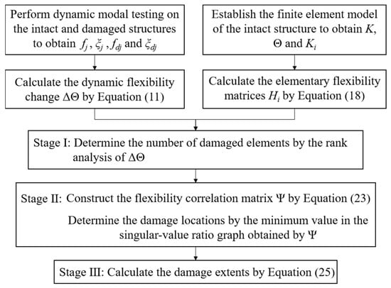
Figure 1.
The flow chart of the complete method.
3. Numerical Example
A numerical example as shown in Figure 2 is used to demonstrate the proposed method. The structure is composed of 27 steel bars. The physical parameters of the material are: elastic modulus 200 GPa, density 7800 kg/m3, cross-sectional area 1.759 × 10⁻⁴ m2. Structural damage is simulated by assuming elastic modulus reduction in the steel bars. Two damage conditions are considered in this example. The first is a single damage condition, in which element 10 is damaged with 15% elastic modulus reduction. The second is the multiple damage condition in which elements 14 and 19 are damaged with 15% and 20% elastic modulus reductions, respectively. The natural frequencies and mode shapes before and after damage are simulated by structural FEM vibration analysis. Table 1 presents the first five natural frequencies without noise for the undamaged and damaged status.
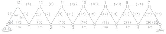
Figure 2.
Numerical model of the 27-bar truss structure.

Table 1.
Natural frequencies without noise for the undamaged and damaged structures (unit: Hz).
3.1. Single Damage Condition
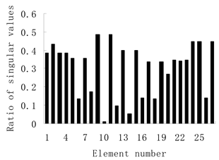
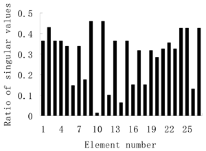
Using the exact modal data, the eigenvalues of for the single damage case can be calculated as: 1.211 × 10⁻⁷, . It was found that only the first eigenvalue is nonzero. Thus, the rank of can be determined as 1 for this damage case. It can be judged in Stage I that only one bar is damaged. Subsequently, Table 2 presents the singular-values of for each element in Stage II. The identified column ranks for each element are also given in Table 2. Note that element 10 corresponds to the minimum column rank. Therefore, it can be judged in Stage II that only the tenth bar is damaged. From Table 2, the ratio of the second singular value to the first singular value can also be used to determine the damage locations more conveniently. Taking the element number as the abscissa and the corresponding ratio as the ordinate, Figure 3 presents the ratio graph of singular values in Table 2. It can be seen from Figure 3 that element 10 corresponds to the minimum ratio of 0. This also means that element 10 is the damaged bar in the structure. Finally, the damage extent can be calculated in Stage III as = 17.65%, which is very close to the true value, 15%.
Table 2.
The singular-values of the flexibility correlation matrix for each element.
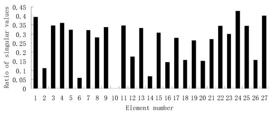
Figure 3.
The singular-value ratio graph obtained by Table 2 when element 10 is damaged (no noise).
Next, the random noise is added in the exact data to simulate the measurement errors in engineering practice. The formula for adding noise follows
where and are the contaminated frequency and mode shapes with noise, is the noise level, and is a random number in the interval [−1, 1]. Moreover, the proposed method is compared with the generalized flexibility method [20,21,22] by using the same contaminated data. To this end, the main formulas of the generalized flexibility method [20,21,22] are briefly reviewed as follows.
First, the generalized flexibility and its sensitivity to the perturbation coefficient are given as
where is the mass matrix of structural FEM. Similar to Equation (11), the generalized flexibility change before and after damage can also be approximately obtained by the low-order vibration eigenpairs as
Comparing Equations (11) and (32), note that the power of frequencies for the generalized flexibility is 4 and the power of frequencies for the ordinary flexibility is 2. This difference gives the generalized flexibility method the advantage that the adverse effect of truncating higher-order modes can be reasonably reduced. On the other hand, the generalized flexibility change can be expressed by the first-order Taylor’s series expansion as
From Equation (33), the damage parameters () can be calculated by solving the linear system of Equation (33). According to the calculated , damage locations and extents can be determined by the generalized flexibility method.
Using the contaminated data, Figure 4 presents the calculated damage extents by the generalized flexibility method for 5% and 10% noise levels, respectively. For comparison, Table 3 provides the damage assessment results by the proposed method.
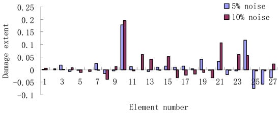
Figure 4.
The calculated damage extents by the generalized flexibility method when element 10 is damaged.
Table 3.
The damage assessment results by the proposed multiple-stage dynamic flexibility analysis method when element 10 is damaged.
In Figure 4, the calculated damage extents of element 10 by the generalized flexibility method are = 17.76% (5% noise level) and = 19.49% (10% noise level). Note that element 10 can be determined as the most possible damaged element since it has the largest value among the calculated damage extents in Figure 4. However, several other elements are misjudged as the damaged elements because they also have relatively large values among the calculated damage extents. Generally, the element can be determined as the possible damaged element if its calculated damage extent is greater than 0.05. From Figure 4, when 5% noise level is considered, element 24 is misjudged as the damaged element since its calculated damage extent is = 11.63%. When 10% noise is considered, elements 12, 15, 21, 23, and 24 are misjudged as the damaged elements since their calculated damage extents are = 6.1%, = 5.12%, = 10.67%, = 5.99%, and = 5.56%. These results show that the generalized flexibility method is prone to misjudgment with the increase in noise level. In Table 3, it can be judged by the proposed method that element 10 is the only damaged element for both noise levels. This means that the proposed method has better antinoise ability than the generalized flexibility method since the misjudgment is avoided. The calculated damage extents of element 10 by the proposed method are = 18.87% (5% noise level) and = 20.32% (10% noise level), which are close to the true value of 15%. Note that the reason for the deviation between the calculated value and the true value of damage extent lies in two aspects. One is the data noise. The other is the operation of ignoring the second-order product in Equation (13).
3.2. Multiple Damage Condition
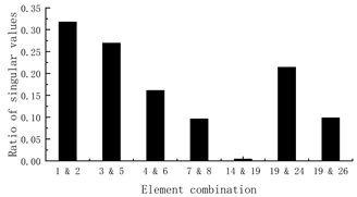
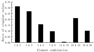
For the multiple damage condition, the eigenvalues of can be calculated by the simulated modal data without noise as: 1.34 × 10⁻⁷, 0.076 × 10⁻⁷, . It was found that the first two eigenvalues are nonzero. Thus, the rank of can be determined as 2 for this damage case. It can be judged in Stage I that two bars were damaged. Subsequently, the singular-values of for every possible element combination can be computed in Stage II. Given space limitations, Table 4 presents the singular-values of some element combinations and the corresponding identified column ranks. From Table 4, the ratio of the third singular value to the first singular value can also be used to determine the damage locations more conveniently. Taking the element combination as the abscissa and the corresponding ratio as the ordinate, Figure 5 presents the ratio graph of singular values in Table 4. It can be seen from Figure 5 that the combination of elements 14 and 19 corresponds to the minimum ratio of 0. Therefore, it can be judged in Stage II that elements 14 and 19 are both damaged. Finally, the damage extents can be calculated in Stage III as = 17.65% and = 25.0%, which are close to the true values, 15% and 20%.
Table 4.
The singular-values of the flexibility correlation matrix for some element combinations.
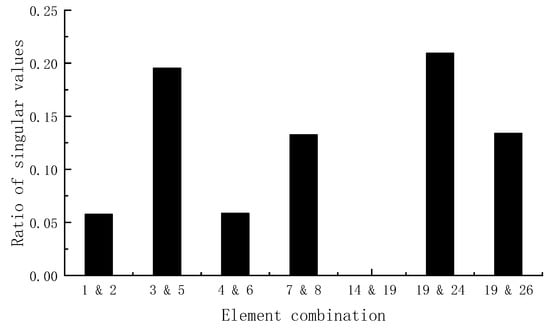
Figure 5.
The singular-value ratio graph obtained by Table 4 when elements 14 and 19 are damaged (no noise).
When 5% and 10% data noise are considered, Figure 6 presents the calculated damage extents by the generalized flexibility method. For comparison, Table 5 provides the damage assessment results by the proposed method.
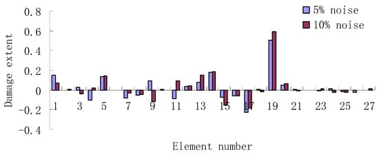
Figure 6.
The calculated damage extents by the generalized flexibility method when elements 14 and 19 are damaged.
Table 5.
The damage assessment results by the proposed multiple-stage dynamic flexibility analysis method when elements 14 and 19 are damaged.
In Figure 6, the calculated damage extents of elements 14 and 19 by the generalized flexibility method are = 17.75% and = 50.69% (5% noise level), and = 18.87% and = 59.08% (10% noise level). Note that elements 14 and 19 can be determined as the most possible damaged elements since they have the larger values among the calculated damage extents shown in Figure 6. However, several other elements are misjudged as the damaged elements because they also have relatively large values among the calculated damage extents. From Figure 6, when 5% noise level is considered, elements 1, 5, 9, 13, and 20 are misjudged as the damaged elements since their calculated damage extents are = 15.28%, = 13.82%, = 9.33%, = 7.89%, and = 5.15%. When 10% noise is considered, elements 1, 5, 11, 13, and 20 are misjudged as the damaged elements since their calculated damage extents are = 6.9%, = 13.93%, = 9.47%, = 15.17%, and = 6.36%. These results again show that the generalized flexibility method is prone to misjudgment with the increase in noise level. In Table 5, it can be judged by the proposed method that only elements 14 and 19 are the two damaged elements for both noise levels. This once again shows that the proposed method has good anti-noise ability. The calculated damage extents by the proposed method are = 18.34% and = 24.92% (5% noise level), and = 17.64% and = 34.71% (10% noise level). It is clear that the damage extents calculated by the proposed method are closer to the true values (15% and 20%) than those calculated by the generalized flexibility method.
For this numerical example, the results show that the generalized flexibility method misjudges the damaged elements, but the proposed method accurately identifies structural damages when the data contain noise. The average calculation error of this method is reduced to about one-third of that of the generalized flexibility method. It was shown that the calculation reliability and accuracy of this method are both higher than those of the generalized flexibility method.
4. Verification by the Experimental Data of Reference
The damage assessment technique presented is further validated using the experimental modal data of a three-floor steel frame structure, conducted by Li in reference [32]. The structural dimensions and damage cases can be seen in reference [32] or in Figure 7. As shown in Figure 7, the main components of this experimental structure are three steel plates and four rectangular columns. Plates and columns are rigidly connected by welding. Structural damages were produced by cutting part of the steel columns for the first and second story. For damage case 1, the width of the cross-section at the column bottom of the first floor is reduced by cutting from 75 to 51.3 mm. Using the cross-section size after cutting, the story stiffness of the first floor is calculated and compared with the story stiffness before cutting. Then, the damage extent for damage case 1 can be obtained as about 11.6% by the ratio of the story stiffness before and after cutting. For damage case 2, the widths of the cross-sections at the column bottoms for the first and second floors are both reduced by cutting from 75 to 37.46 mm. The corresponding damage extents for damage case 2 can also be calculated as about 21.1% by the ratio of the story stiffness before and after cutting. The intact and damaged models were placed on a shaking table to test the dynamic characteristics. The shaking table produced white noise in the frequency range 1–30 Hz in the X direction. The peak acceleration of the excitation was taken as 0.05 g. The duration of the excitation was 180 s. The B&K 4370 acceleration sensors were set at each floor to measure the accelerations in the X direction. The time signals were sampled at 300 Hz and modulated by the B&K 2635. Using the Structural Vibration Solutions ARTeMIS software, the time signals obtained were analyzed by the frequency domain decomposition method to obtain the three natural frequencies of the frame model. Table 6, Table 7 and Table 8 present the testing modal data in reference [32] for the undamaged and damaged structures.
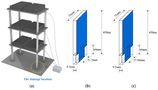
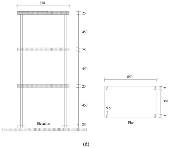
Figure 7.
Experimental model of a three-floor steel frame structure. (a) Schematic diagram of the experimental structure in reference [32]; (b) Damage case 1: notch by cutting from 75 to 51.3 mm in the first floor; (c) Damage case 2: notches by cutting from 75 to 37.46 mm in the first and second floors; (d) Geometric size of the experimental structure.
Table 6.
Experimental modal data for the undamaged structure.
Table 7.
Experimental modal data for damage case 1 (the first floor is damaged by 11.6% stiffness reduction).
Table 8.
Experimental modal data for damage case 2 (the first and second floors are both damaged by 21.1% stiffness reductions).
4.1. Damage Case 1
The damage assessment results obtained by the proposed method and the generalized flexibility method are both presented in Table 9 for comparison.
Table 9.
The damage assessment results by the proposed method and the generalized flexibility method for damage case 1 of the experimental structure.
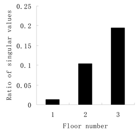
From Table 9, note that both methods can successfully identify the damage in the first floor. The damage extent calculated by the proposed method and the generalized flexibility method are 13.11% and 17.89%, respectively. Compared to the latter, the former is closer to the true value of 11.6%.
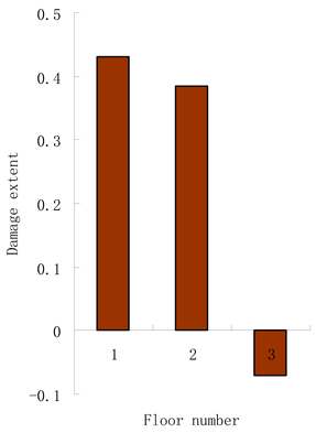
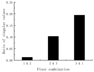
4.2. Damage Case 2
Table 10 presents the damage assessment results by the proposed method and the generalized flexibility method for damage case 2 of the experimental structure. From Table 10, it has been shown that both methods can successfully identify the damages in the first and second floors. Compared with the true values 21.1%, the calculated damage extent by the proposed method has higher accuracy than those by the generalized flexibility method.
Table 10.
The damage assessment results by the proposed method and the generalized flexibility method for damage case 2 of the experimental structure.
For damage case 1, the relative errors of the damage extent calculated by the proposed method and the generalized flexibility method are 13% and 54%, respectively. The calculation error of this method is reduced to one-fourth of that of the generalized flexibility method. For damage case 2, the relative errors of the damage extent calculated by the proposed method and the generalized flexibility method are 59% and 104% for the first floor, and 27% and 82% for the second floor, respectively. The calculation errors for the first and second floors by this method are reduced to a half and one-third of those of the generalized flexibility method. These results show that the calculation accuracy of this method is significantly higher than that of the generalized flexibility method.
5. Conclusions
In this work, a damage identification algorithm is proposed for detecting structural damage by using multiple-stage dynamic flexibility analysis. The proposed algorithm can be divided into three stages. In Stage I, the number of damaged elements in the structure can be initially determined by the rank of dynamic flexibility change. In Stage II, damage locations can be determined by the minimum rank of the flexibility correlation matrix. In Stage III, the damage extent of the damaged elements can be obtained. The proposed method is verified by a numerical example and an experimental structure. From the numerical and experimental results, it is found that structure damages can be successfully identified through multiple-stage dynamic flexibility analysis.
The remarkable advantage of the proposed method is that it can obtain stable and accurate damage assessment results without misjudgment even if the data contain much noise. By comparative study, the proposed method performs better than the generalized flexibility method in the numerical and experimental examples. It was shown that the proposed method has powerful antinoise ability in damage assessment. It is noted that this algorithm may also be applied to assess other damage types such as cracking and delamination, provided there are observable changes in the dynamic parameters before and after damage. In addition, it should be pointed out that the proposed method has the following disadvantages. One is that this algorithm can assess only notable stiffness decrease in the structure. It is difficult to identify the damage that does not cause a significant reduction in structural stiffness. The other disadvantage is that nonlinear vibration is not considered in the proposed method if structural damage is relatively large. All the theoretical derivation of this work is based on linear structural systems for the intact and damaged structures. If nonlinear vibration occurs in the structure due to damage, the proposed method must be improved in some aspects before it can be used. More theoretical research and engineering applications can be carried out in the future to verify the applicability of this method to other special damage conditions.
Author Contributions
Methodology, Y.S. and Q.Y.; Software, Y.S., Q.Y. and X.P.; Validation, Y.S., Q.Y. and X.P. All authors have read and agreed to the published version of the manuscript.
Funding
This work is supported by the public welfare technology application research project of Zhejiang Province, China (LGF22E080021), Natural Science Foundation of China (52008215), the Natural Science Foundation of Zhejiang Province, China (LQ20E080013), the major special science and technology project (2019B10076) of ”Ningbo science and technology innovation 2025”, and Ningbo natural science foundation project (202003N4169).
Institutional Review Board Statement
Not applicable.
Informed Consent Statement
Not applicable.
Data Availability Statement
The data used to support the findings of this study are included within the article and also available from the corresponding author upon request.
Conflicts of Interest
The authors declare that there are no conflicts of interest.
References
- Roeck, G.D. The state-of-the-art of damage detection by vibration monitoring: The SIMCES experience. J. Struct. Control. 2003, 10, 127–134. [Google Scholar] [CrossRef]
- Yan, Y.J.; Cheng, L.; Wu, Z.Y.; Yam, L.H. Development in vibration-based structural damage detection technique. Mech. Syst. Signal Processing 2007, 21, 2198–2211. [Google Scholar] [CrossRef]
- Cruz, P.J.S.; Salgado, R. Performance of vibration-based damage detection methods in bridges. Comput. -Aided Civ. Infrastruct. Eng. 2009, 24, 62–79. [Google Scholar] [CrossRef]
- Avci, O.; Abdeljaber, O.; Kiranyaz, S.; Hussein, M.; Gabbouj, M.; Inman, D.J. A review of vibration-based damage detection in civil structures: From traditional methods to Machine Learning and Deep Learning applications. Mech. Syst. Signal Process. 2021, 147, 107077. [Google Scholar] [CrossRef]
- Vestroni, F.; Capecchi, D. Damage detection in beam structures based on frequency measurements. J. Eng. Mech. 2000, 126, 761–768. [Google Scholar] [CrossRef]
- Kessler, S.S.; Spearing, S.M.; Atalla, M.J.; Cesnik, C.E.; Soutis, C. Damage detection in composite materials using frequency response methods. Compos. Part B Eng. 2002, 33, 87–95. [Google Scholar] [CrossRef]
- Hwang, H.Y.; Kim, C. Damage detection in structures using a few frequency response measurements. J. Sound Vib. 2004, 270, 1–14. [Google Scholar] [CrossRef]
- Limongelli, M.P. Frequency response function interpolation for damage detection under changing environment. Mech. Syst. Signal Process. 2010, 24, 2898–2913. [Google Scholar] [CrossRef]
- Bandara, R.P.; Chan, T.H.T.; Thambiratnam, D.P. Structural damage detection method using frequency response functions. Struct. Health Monit. 2014, 13, 418–429. [Google Scholar] [CrossRef]
- Sha, G.; Radzieński, M.; Cao, M.; Ostachowicz, W. A novel method for single and multiple damage detection in beams using relative natural frequency changes. Mech. Syst. Signal Process. 2019, 132, 335–352. [Google Scholar] [CrossRef]
- Kim, J.T.; Ryu, Y.S.; Cho, H.M.; Stubbs, N. Damage identification in beam-type structures: Frequency-based method vs mode-shape-based method. Eng. Struct. 2003, 25, 57–67. [Google Scholar] [CrossRef]
- Qiao, P.; Lu, K.; Lestari, W.; Wang, J. Curvature mode shape-based damage detection in composite laminated plates. Compos. Struct. 2007, 80, 409–428. [Google Scholar] [CrossRef]
- Yazdanpanah1a, O.; Seyedpoor, S.M. A new damage detection indicator for beams based on mode shape data. Struct. Eng. Mech. 2015, 53, 725–744. [Google Scholar] [CrossRef]
- Rucevskis, S.; Janeliukstis, R.; Akishin, P.; Chate, A. Mode shape-based damage detection in plate structure without baseline data. Struct. Control. Health Monit. 2016, 23, 1180–1193. [Google Scholar] [CrossRef]
- Umar, S.; Bakhary, N.; Abidin, A.R.Z. Response surface methodology for damage detection using frequency and mode shape. Measurement 2018, 115, 258–268. [Google Scholar] [CrossRef]
- Catbas, F.N.; Brown, D.L.; Aktan, A.E. Use of modal flexibility for damage detection and condition assessment: Case studies and demonstrations on large structures. J. Struct. Eng. 2006, 132, 1699–1712. [Google Scholar] [CrossRef]
- Sung, S.H.; Koo, K.Y.; Jung, H.J. Modal flexibility-based damage detection of cantilever beam-type structures using baseline modification. J. Sound Vib. 2014, 333, 4123–4138. [Google Scholar] [CrossRef]
- Grande, E.; Imbimbo, M. A multi-stage approach for damage detection in structural systems based on flexibility. Mech. Syst. Signal Process. 2016, 76, 455–475. [Google Scholar] [CrossRef]
- Wickramasinghe, W.R.; Thambiratnam, D.P.; Chan TH, T. Damage detection in a suspension bridge using modal flexibility method. Eng. Fail. Anal. 2020, 107, 104194. [Google Scholar] [CrossRef]
- Li, J.; Wu, B.; Zeng, Q.C.; Lim, C.W. A generalized flexibility matrix based approach for structural damage detection. J. Sound Vib. 2010, 329, 4583–4587. [Google Scholar] [CrossRef]
- Liu, H.; Li, Z. An improved generalized flexibility matrix approach for structural damage detection. Inverse Probl. Sci. Eng. 2020, 28, 877–893. [Google Scholar] [CrossRef]
- Liu, H.; Wu, B.; Li, Z. The generalized flexibility matrix method for structural damage detection with incomplete mode shape data. Inverse Probl. Sci. Eng. 2021, 29, 2019–2039. [Google Scholar] [CrossRef]
- Maizuar, M.; Zhang, L.; Miramini, S.; Mendis, P.; Thompson, R.G. Detecting structural damage to bridge girders using radar interferometry and computational modelling. Struct. Control. Health Monit. 2017, 24, 1–6. [Google Scholar] [CrossRef]
- Alani, A.M.; Aboutalebi, M.; Kilic, G. Use of non-contact sensors (IBIS-S) and finite element methods in the assessment of bridge deck structures. Struct. Concr. 2014, 15, 240–247. [Google Scholar] [CrossRef]
- Raja, B.; Miramini, S.; Duffield, C.; Chen, S.; Zhang, L. A Simplified Methodology for Condition Assessment of Bridge Bearings Using Vibration Based Structural Health Monitoring Techniques. Int. J. Struct. Stab. Dyn. 2021, 21, 2150133. [Google Scholar] [CrossRef]
- Li, W.; Hancock, C.; Yang, Y.; Meng, X. Dynamic deformation monitoring of an offshore platform structure with accelerometers. J. Civ. Struct. Health Monit. 2021, 12, 275–287. [Google Scholar] [CrossRef]
- Zini, G.; Betti, M.; Bartoli, G. A pilot project for the long-term structural health monitoring of historic city gates. J. Civ. Struct. Health Monit. 2022, 12, 537–556. [Google Scholar] [CrossRef]
- Aminullah, A.; Suhendro, B.; Panuntun, R.B. Optimal Sensor Placement for Accelerometer in Single-Pylon Cable-Stayed Bridge. In Proceedings of the 5th International Conference on Sustainable Civil Engineering Structures and Construction Materials; Springer: Singapore, 2022; pp. 63–79. [Google Scholar]
- Cocking, S.; Alexakis, H.; Dejong, M. Distributed dynamic fibre-optic strain monitoring of the behaviour of a skewed masonry arch railway bridge. J. Civ. Struct. Health Monit. 2021, 11, 989–1012. [Google Scholar] [CrossRef]
- Nguyen, T.D.; Nguyen, T.Q.; Nhat, T.N.; Nguyen-Xuan, H.; Ngo, N.K. A novel approach based on viscoelastic parameters for bridge health monitoring: A case study of Saigon bridge in Ho Chi Minn City-Vietnam. Mech. Syst. Signal Process. 2020, 141, 106728.1–106728.17. [Google Scholar] [CrossRef]
- Capilla, J.J.; Au, S.K.; Brownjohn, J.; Hudson, E. Ambient vibration testing and operational modal analysis of monopole telecoms structures. J. Civ. Struct. Health Monit. 2021, 11, 1077–1091. [Google Scholar] [CrossRef]
- Li, L. Numerical and Experimental Studies of Damage Detection for Shear Buildings; Huazhong University of Science and Technology: Wuhan, China, 2005. [Google Scholar]

Publisher’s Note: MDPI stays neutral with regard to jurisdictional claims in published maps and institutional affiliations. |
© 2022 by the authors. Licensee MDPI, Basel, Switzerland. This article is an open access article distributed under the terms and conditions of the Creative Commons Attribution (CC BY) license (https://creativecommons.org/licenses/by/4.0/).