Spacecraft Staring Attitude Control for Ground Targets Using an Uncalibrated Camera

Abstract

Previous staring attitude control techniques utilize the geographic location of a ground target to dictate the direction of the camera’s optical axis, while the assembly accuracy and the internal structure of the spaceborne camera are not considered. This paper investigates the image-based staring controller design of a video satellite in the presence of uncertain intrinsic and extrinsic camera parameters. The dynamical projection model of the ground target on the image plane is firstly established, and then we linearly parameterize the defined projection errors. Furthermore, a potential function and a self-updating rule are introduced to estimate the parameters online by minimizing the projection errors. As the parameters are updating constantly, an adaptive control algorithm is developed, so that the errors between the current and the desired projections of the ground target converge to zero. The stability is proved using Barbalat’s lemma. Simulation results show that the designed controller can successfully move the target’s projection to the desired coordinate even though the camera parameters are unknown.

1. Introduction

With the increasing importance of Earth observation projects, staring imaging outperforms other sensing techniques owing to its unique capability in capturing continuous images of the ground target [1,2]. As its name suggests, staring control requires the camera to constantly point to the target, so we can obtain images where the target is always at the center. To achieve this purpose, the optical axis of the camera is supposed to be aimed at the target throughout the whole observation phase. Many video satellites (e.g., TUBSAT [3], Tiantuo-2, Jilin-1) are equipped with staring mode, therefore they can be applied for various scenarios, such as emergence rescue, target monitoring, and so on [4,5,6]. In a staring control case, the satellite is moving along the orbit and simultaneously the ground target is not stationary as it is fixed on the rotating Earth’s surface, leading to a time-varying relative motion. Therefore, a dedicated attitude controller should be designed to keep the satellite staring at the target.

Conventional methods for staring control mainly require the relative position between the satellite and the target, normally obtained via orbital data and the geographic information, respectively. Furthermore, a staring imaging for a single point dictates only the optical axis, so the orientation perpendicular to it is free. Refs. [2,7] both propose PD-like controllers to achieve staring imaging, while Refs. [8,9,10] pursue optimality during the attitude maneuver. Ref. [11] realizes a similar real-time optimal control method with an emphasis on the pointing accuracy. However, the above studies have not considered the image feedback, though the image error directly and precisely reflects the controller’s accuracy. In light of this, it is necessary to take use of the camera’s ability to achieve more precise staring.

Besides traditional methods whose attitude control torques are generated by establishing the inertial geometry and disintegrating the relative orientation into different rotation angles, state-of-the-art image-processing technologies [12,13,14,15] have made it possible to develop a novel image-based staring controller relying on the target’s projection on the image plane. As a camera plays an essential role in different engineering applications [16,17,18,19,20,21,22], various image-based control methods have been developed. The same as staring control, some of these control schemes use the image to obtain the orientation of the target point. For example, Refs. [23,24] study positioning control of robots, Ref. [25] conducts research on motion control of an unmanned aerial vehicle (UAV), and Ref. [26] uses images for space debris tracking. However, above studies either neglect the uncertainties of the camera or do not consider the spacecraft kinematics and dynamics. A spaceborne camera is hard to calibrate in a complicated working environment such as space; therefore, this paper focuses on analyzing an image-based adaptive staring attitude controller for a video satellite using an uncalibrated camera.

To take advantage of the images, the projection model should be analyzed. The target’s projection on the image plane is decided by the relative position between the target and satellite in the inertial space, the satellite’s attitude and the camera’s configuration. The camera configuration consists of the intrinsic structure and the extrinsic mounting position and orientation. Camera parameters are to be properly defined, thus able to be linearized and thereafter estimated online. Worth noting that the relative orientation of staring imaging is influenced by both the attitude and orbital motion, which is different from a robotic model. To conclude the discussion, for a video satellite whose camera is uncalibrated, the image-based staring attitude controller is built upon the thorough analysis of the camera structure.

This paper differs from traditional staring attitude control methods by focusing on the image-based adaptive algorithm accommodating the unknown camera parameters, therefore the kinematic relationship between the image and the attitude is firstly established. Through linear parameterization, the negative gradients of the projection errors are chosen as the direction of parameter adjustment. Estimated parameters and the image information are then adopted to formulate the staring controller, which directs the target’s projection to the desired coordinates. A potential function is also introduced to guarantee the controller’s stability. The convergence of the ground target’s projection to its desired location indicates that the optical axis reaches the desired orientation. Finally, simulation shows the trajectory of the projection on the image plane. As the projection moves along the trajectory, the image errors, as well as the estimated projection errors, are approaching zero.

The remainder of this paper is organized as follows. The camera modeling is introduced in Section 2, where the projection kinematics are derived for a video satellite. In Section 3, we propose the adaptive controller, including the parameter extraction and estimation. Simulation is presented in Section 4 and the results demonstrate the effectiveness of our controller. Conclusions are drawn in the last section.

2. Problem Formulation

This section starts with a brief introduction of satellite attitude kinematics and dynamics, and then establishes the camera projection model between the target’s position in the Earth-centered inertial (ECI) frame and its pixel coordinates on the image plane. Finally, the projection kinematics in the form of pixel coordinates are derived.

2.1. Attitude Kinematics and Dynamics

A quaternion q, which includes a scalar part $q_0$ and a vector part ${\mathit{q}}_v={\left(q_1{q}_2{q}_3\right)}^T$, is adopted to describe the attitude:

$$q=cos\left(\varphi /2\right)+\mathit{r}sin\left(\varphi /2\right)=q_0+{\mathit{q}}_v$$

(1)

where $\mathit{r}$ is the Euler axis and $\varphi$ is the rotation angle. The quaternion can avoid the singularity of Euler angles and it must meet the normalization condition: $∥q∥=1$. The attitude kinematics and dynamics of a satellite as a rigid body are given by

$$\begin{array}{cc}\hfill \left[\begin{array}{c}{\dot{\mathit{q}}}_v\\ {\dot{q}}_0\end{array}\right]& =\frac{1}{2}\left[\begin{array}{c}{q}_0{E}_3+sk\left({\mathit{q}}_v\right)\\ -{\mathit{q}}_v^T\end{array}\right]\mathit{\omega }\hfill \\ \hfill J\dot{\mathit{\omega }}& =-\mathit{\omega }\times J\mathit{\omega }+\mathit{U}\hfill \end{array}$$

(2)

where $E_3$ is a $3\times 3$ unit matrix, J is the inertial moment of the satellite and $\mathit{\omega }$ represents the angular velocity of the satellite relative to the inertial frame expressed in the body frame. $\mathit{U}$ is the attitude control torques. The operation $sk\left(·\right)$ is defined as

$$sk\left({\mathit{q}}_v\right)=\left[\begin{array}{c}\begin{array}{ccc}0& -q_3& q_2\end{array}\\ \begin{array}{ccc}{q}_3& 0& -q_1\end{array}\\ \begin{array}{ccc}-q_2& q_1& 0\end{array}\end{array}\right]$$

(3)

In traditional attitude tracking controllers including the staring control, a desired quaternion $q_d$ should firstly be designed and then the error quaternion $q_e$ is obtained. According to different control strategies, $\mathit{U}$ is calculated based on $q_e$ and the angular velocity error ${\mathit{\omega }}_e$. For an image-based staring control case, alternative attitude representation is needed as the attitude errors are embodied in the image errors, i.e., the pixel coordinate errors between the current and desired projection. Therefore, we are to measure the relative attitude via image recognition. Inevitably, an uncalibrated camera introduces extra uncertainties into the images. For this reason, the analysis of a camera model is necessary.

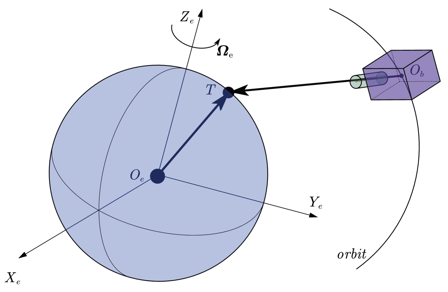
2.2. Earth-Staring Observation

Earth-staring observation requires the camera’s optical axis to point towards the ground target for a period of time. The scenario is shown in Figure 1. $O_e-X_e{Y}_e{Z}_e$ is ECI frame. $O_e$ and $O_b$ are the the center of mass of Earth and the satellite, respectively. The satellite with a camera is on the orbit, and the ground target T is located at the Earth surface while rotating around $Z_e$ at the angular velocity of ${\Omega }_{\mathit{e}}$. The satellite’s position is expressed in ECI as ${\mathit{R}}_{eb}$, and ${}_i{}^{b}M$ represents the rotation matrix from ECI to the body frame. Define the homogeneous transform matrix from the inertial frame to the body frame $T_h\in {\mathbb{R}}^{4\times 4}$:

$$T_h=\left(\begin{array}{cc}{}_i{}^{b}M& -{{}_i{}^{b}M}^i{\mathit{R}}_{eb}\\ {\mathbf{0}}_{1\times 3}& 1\end{array}\right)$$

(4)

${}^i{\mathit{R}}_{eT}$ is the target’s position in ECI, and ${}^b{\mathit{R}}_{bT}$ is the vector from the satellite to the target expressed in the body frame. Homogeneous coordinates are adopted to better describe the transformation. According to the geometrical relationship, we have

$$\left(\begin{array}{c}{}^b{\mathit{R}}_{bT}\\ 1\end{array}\right)=T_h\left(\begin{array}{c}{}^i{\mathit{R}}_{eT}\\ 1\end{array}\right)$$

(5)

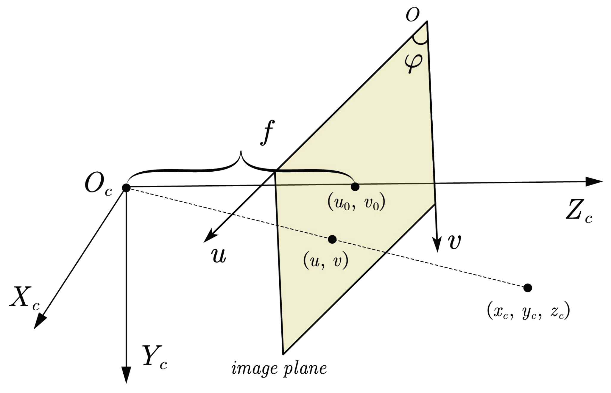
2.3. The Intrinsic Camera Model

Inside the camera, the target is projected on the image plane through the lens. Assume the camera has a focal length of f and a pixel size of $dx\times dy$. Figure 2 depicts the camera frame $O_c-X_c{Y}_c{Z}_c$ and the 2D pixel frame $o-uv$, whose conjunction with the optical axis is ${\left(u_0,v_0\right)}^T$. $\phi$ is the angle between the axis u and v. The target in the camera frame is expressed as ${}^c{\mathit{R}}_{cT}={\left(x_c,y_c,z_c\right)}^T$, and its projection is $\mathit{y}={\left(u,v\right)}^T$. Thus, we have the following projection transformation:

$$z_c\left(\begin{array}{c}\mathit{y}\\ 1\end{array}\right)=\Pi \left(\begin{array}{c}{}^c{\mathit{R}}_{cT}\\ 1\end{array}\right)$$

(6)

where $\Pi \in {\mathbb{R}}^{3\times 4}$ is defined as

$$\Pi =\left(\begin{array}{ccc}f/dx& -f/dx·cot\phi & \begin{array}{cc}{u}_0& 0\end{array}\\ 0& f/\left(dy·sin\phi \right)& \begin{array}{cc}{v}_0& 0\end{array}\\ 0& 0& \begin{array}{cc}1& 0\end{array}\end{array}\right)$$

(7)

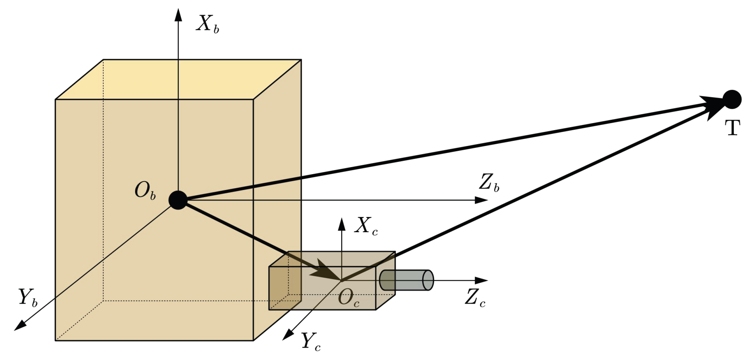
2.4. The Extrinsic Camera Model

The position and attitude of the camera frame $O_c-X_c{Y}_c{Z}_c$ with respect to the body frame $O_b-X_b{Y}_b{Z}_b$ is displayed in Figure 3. ${\mathit{R}}_{bc}$ represents the position of $O_c$ in the body frame. Similarly, we define the homogeneous transform matrix from the body frame to the camera frame $T\in {\mathbb{R}}^{4\times 4}$:

$$T=\left(\begin{array}{cc}{}_b{}^{c}M& {-}^c{\mathit{R}}_{bc}\\ {\mathbf{0}}_{1\times 3}& 1\end{array}\right)$$

(8)

The target’s position in the camera frame is ${}^c{\mathit{R}}_{cT}$ and in the body frame it is ${}^b{\mathit{R}}_{bT}$. The transformation between them can be given by

$$\left(\begin{array}{c}{}^c{\mathit{R}}_{cT}\\ 1\end{array}\right)=T·\left(\begin{array}{c}{}^b{\mathit{R}}_{bT}\\ 1\end{array}\right)$$

(9)

2.5. The Projection Kinematics of Staring Imaging

According to Equations (6) and (9), we have

$$z_c\left(\begin{array}{c}\mathit{y}\\ 1\end{array}\right)=N·\left(\begin{array}{c}{}^b{\mathit{R}}_{bT}\\ 1\end{array}\right)$$

(10)

where the projection matrix $N\in {\mathbb{R}}^{3\times 4}$ is defined by $N=\Pi ·T$ and its elements are denoted as $n_{ij}$ $\left(i=1,2,3;j=1,2,3,4\right)$. Then combine (5) and (10), we obtain

$$\left(\begin{array}{c}\mathit{y}\\ 1\end{array}\right)=\frac{1}{z_c}N·T_h·\left(\begin{array}{c}{}^i{\mathit{R}}_{eT}\\ 1\end{array}\right)$$

(11)

The above equation reveals the mapping relation between the target’s position in ECI and its projection coordinates on the image plane. The matrix N reflects the camera’s role in the transformation, while T contains the satellite’s attitude and orbit motion impacts. Define

$$N\triangleq \left(\begin{array}{c}{\mathit{n}}_1^T\\ {\mathit{n}}_2^T\\ {\mathit{n}}_3^T\end{array}\right)\triangleq \left(\begin{array}{c}\mathit{P}\\ {\mathit{n}}_3^T\end{array}\right)$$

(12)

where $\mathit{P}\in {\mathbb{R}}^{2\times 4}$ is the matrix consisting of the first two rows of N, and ${\mathit{n}}_3^T\in {\mathbb{R}}^{1\times 4}$ is the third row. To derive the kinematic equations more clearly, we will explicitly denote the time-varying states. Equation (11) can be rewritten as

$$\begin{array}{cc}\hfill \mathit{y}\left(t\right)& =\frac{1}{z_c\left(t\right)}\mathit{P}·T_h\left(t\right)·\left(\begin{array}{c}{}^i{\mathit{R}}_{eT}\left(t\right)\\ 1\end{array}\right)\hfill \\ \hfill z_c\left(t\right)& ={\mathit{n}}_3^T·T_h\left(t\right)·\left(\begin{array}{c}{}^i{\mathit{R}}_{eT}\left(t\right)\\ 1\end{array}\right)\hfill \end{array}$$

(13)

For simplicity, let ${\mathit{n}}_{3\left(3\right)}^T$ denote a vector formed by the first three elements of ${\mathit{n}}_3^T$, and let ${\mathit{P}}_{\left(3\right)}$ denote a matrix formed by the first three columns of $\mathit{P}$. Differentiate the depth $z_c\left(t\right)$ of the target in the camera frame and we obtain

$$\begin{array}{cc}\hfill {\dot{z}}_c\left(t\right)=& {\mathit{n}}_3^T\left(\begin{array}{cc}sk\left({}_i{}^{b}M\left(t\right){{}^i\mathit{R}}_{eT}\left(t\right)-{}_i{}^{b}M\left(t\right){{}^i\mathit{R}}_{eb}\left(t\right)\right)& -{}_i{}^{b}M\left(t\right)\\ {\mathbf{0}}_{1\times 3}& {\mathbf{0}}_{1\times 3}\end{array}\right)\left(\begin{array}{c}\mathit{\omega }\left(t\right)\\ {}^i{\mathit{V}}_{eb}\left(t\right)\end{array}\right)\hfill \\ & +{\mathit{n}}_3^T{T}_h\left(t\right)\left(\begin{array}{c}{}^i{\mathit{V}}_{eT}\left(t\right)\\ 0\end{array}\right)\hfill \\ \hfill =& \left(\begin{array}{cc}{\mathit{n}}_{3\left(3\right)}^T& n_{34}\end{array}\right)\left(\begin{array}{cc}sk\left({}_i{}^{b}M\left(t\right){{}^i\mathit{R}}_{eT}\left(t\right)-{}_i{}^{b}M\left(t\right){{}^i\mathit{R}}_{eb}\left(t\right)\right)& -{}_i{}^{b}M\left(t\right)\\ {\mathbf{0}}_{1\times 3}& {\mathbf{0}}_{1\times 3}\end{array}\right)\left(\begin{array}{c}\mathit{\omega }\left(t\right)\\ {}^i{\mathit{V}}_{eb}\left(t\right)\end{array}\right)\hfill \\ \hfill & +\left(\begin{array}{cc}{\mathit{n}}_{3\left(3\right)}^T& n_{34}\end{array}\right)\left(\begin{array}{cc}{}_i{}^{b}M\left(t\right)& -{}_i{}^{b}M\left(t\right){{}^i\mathit{R}}_{eb}\left(t\right)\\ {\mathbf{0}}_{1\times 3}& 1\end{array}\right)\left(\begin{array}{c}{}^i{\mathit{V}}_{eT}\left(t\right)\\ 0\end{array}\right)\hfill \\ \hfill =& {\mathit{n}}_{3\left(3\right)}^T\left(\begin{array}{cc}sk\left({}_i{}^{b}M\left(t\right){{}^i\mathit{R}}_{eT}\left(t\right)-{}_i{}^{b}M\left(t\right){{}^i\mathit{R}}_{eb}\left(t\right)\right)& -{}_i{}^{b}M\left(t\right)\end{array}\right)\left(\begin{array}{c}\mathit{\omega }\left(t\right)\\ {}^i{\mathit{V}}_{eb}\left(t\right)\end{array}\right)\hfill \\ \hfill & +{\mathit{n}}_{3\left(3\right)}^T{}_i{}^{b}M\left(t\right)·{{}^i\mathit{V}}_{eT}\left(t\right)\hfill \\ \hfill =& {\mathit{n}}_{3\left(3\right)}^{T}sk\left({}_i{}^{b}M\left(t\right){{}^i\mathit{R}}_{eT}\left(t\right)-{}_i{}^{b}M\left(t\right){{}^i\mathit{R}}_{eb}\left(t\right)\right)\mathit{\omega }\left(t\right)\hfill \\ \hfill & +{\mathit{n}}_{3\left(3\right)}^T{}_i{}^{b}M\left(t\right)\left({}^i{\mathit{V}}_{eT}\left(t\right)-{{}^i\mathit{V}}_{eb}\left(t\right)\right)\hfill \end{array}$$

(14)

To simplify the expression, we define

$$\begin{array}{cc}\hfill a\left(t\right)=& {\mathit{n}}_{3\left(3\right)}^{T}sk\left({}_i{}^{b}M\left(t\right){}^i{\mathit{R}}_{eT}\left(t\right)-{}_i{}^{b}M\left(t\right){{}^i\mathit{R}}_{eb}\left(t\right)\right)\hfill \\ \hfill a_v\left(t\right)=& {\mathit{n}}_{3\left(3\right)}^T{}_i{}^{b}M\left(t\right)\left({}^i{\mathit{V}}_{eT}\left(t\right)-{{}^i\mathit{V}}_{eb}\left(t\right)\right)\hfill \end{array}$$

(15)

Thus we have

$${\dot{z}}_c\left(t\right)=a\left(t\right)\mathit{\omega }\left(t\right)+a_v\left(t\right)$$

(16)

Similarly, we define

$$\begin{array}{cc}\hfill A\left(t\right)=& \left({\mathit{P}}_{\left(3\right)}-\mathit{y}\left(t\right){\mathit{n}}_{3\left(3\right)}^T\right)sk\left({}_i{}^{b}M\left(t\right){{}^i\mathit{R}}_{eT}\left(t\right)-{}_i{}^{b}M\left(t\right){{}^i\mathit{R}}_{eb}\left(t\right)\right)\hfill \\ \hfill A_v\left(t\right)=& \left({\mathit{P}}_{\left(3\right)}-\mathit{y}\left(t\right){\mathit{n}}_{3\left(3\right)}^T\right){}_i{}^{b}M\left(t\right)\left({}^i{\mathit{V}}_{eT}\left(t\right)-{{}^i\mathit{V}}_{eb}\left(t\right)\right)\hfill \end{array}$$

(17)

then we have the derivative of the image coordinates given by

$$\begin{array}{cc}\hfill \dot{\mathit{y}}\left(t\right)=& \frac{1}{z_c\left(t\right)}\mathit{P}·{\dot{T}}_h\left(t\right)·\left(\begin{array}{c}{}^i{\mathit{R}}_{eT}\left(t\right)\\ 1\end{array}\right)-\frac{{\dot{z}}_c\left(t\right)}{z_c\left(t\right)}\mathit{y}\left(t\right)+\frac{1}{z_c\left(t\right)}\mathit{P}·T_h\left(t\right)·\left(\begin{array}{c}{}^i{\mathit{V}}_{eT}\left(t\right)\\ 1\end{array}\right)\hfill \\ \hfill =& \frac{1}{z_c\left(t\right)}\left({\mathit{P}}_{\left(3\right)}-\mathit{y}\left(t\right){\mathit{n}}_{3\left(3\right)}^T\right)sk\left({}_i{}^{b}M\left(t\right){{}^i\mathit{R}}_{eT}\left(t\right)-{}_i{}^{b}M\left(t\right){{}^i\mathit{R}}_{eb}\left(t\right)\right)\mathit{\omega }\hfill \\ \hfill & +\frac{1}{z_c\left(t\right)}\left({\mathit{P}}_{\left(3\right)}-\mathit{y}\left(t\right){\mathit{n}}_{3\left(3\right)}^T\right){}_i{}^{b}M\left(t\right)\left({}^i{\mathit{V}}_{eT}\left(t\right)-{{}^i\mathit{V}}_{eb}\left(t\right)\right)\hfill \\ \hfill =& \frac{1}{z_c\left(t\right)}\left[A\left(t\right)\mathit{\omega }\left(t\right)+A_v\left(t\right)\right]\hfill \end{array}$$

(18)

Equations (16) and (18) are the staring imaging kinematics. From the prior information of the target point, the position ${}^i{\mathit{R}}_{eT}\left(t\right)$ and velocity ${}^i{\mathit{V}}_{eT}\left(t\right)$ of the ground point are already known. Moreover, noting that the attitude and orbit determination can provide the rotation matrix ${}_i{}^{b}M\left(t\right)$ and the orbital location ${}^i{\mathit{R}}_{eb}\left(t\right)$ and velocity ${}^i{\mathit{V}}_{eb}\left(t\right)$, the only uncertain parameters are ${\mathit{P}}_{\left(3\right)}$ and ${\mathit{n}}_{3\left(3\right)}^T$. There are a few characteristics worth analyzing in the kinematic equations. First, the depth $z_c\left(t\right)$ is not observable through images, therefore our controller can not access depth information. Second, the matrices $a_v\left(t\right)$ and $A_v\left(t\right)$ contain the relative orbital motion and are uncontrollable, and simultaneously we do not conduct orbit maneuver. This brings in a problem that if the relative motion between the target and the satellite is too fast, the demand to track the target may exceed the satellite’s attitude maneuver capability. This can result in the target being lost in the field of view. Hence, the satellite should have sufficient angular maneuver capability to keep up the relative rotation. Moreover, refer to [2] for more analysis of the relative angular velocity. Third, the image-based kinematics (16) and (18) maintain the same feature as quaternion-based kinematics (2) as they are all linear with regard to $\mathit{\omega }$. Fourth, the unknown camera parameters exist in $a_v\left(t\right)$, $a_v\left(t\right)$, $A\left(t\right)$ and $A_v\left(t\right)$, so no accurate projection change rate can be derived through the kinematics, and a self-updating rule is to be proposed to estimate them online.

2.6. Control Objective

The control objective is to guarantee the projection coordinate $\mathit{y}\left(t\right)$ approaches its desired location ${\mathit{y}}_d$ on the image plane. The $\mathit{y}\left(t\right)$ is extracted from the real-time images and ${\mathit{y}}_d$ is predetermined. Normally we expect to fix the target point at the center of the image to gain a better view, thus without loss of generality, ${\mathit{y}}_d={\left(u_0,v_0\right)}^T$ is selected. To realize this purpose, an adaptive controller is to be designed to specifically address the camera parameters. Define the image error $\Delta \mathit{y}\left(t\right)=\mathit{y}\left(t\right)-{\mathit{y}}_d$, the control objective is that $\Delta \mathit{y}\left(t\right)$ asymptotically converges to $\mathbf{0}$.

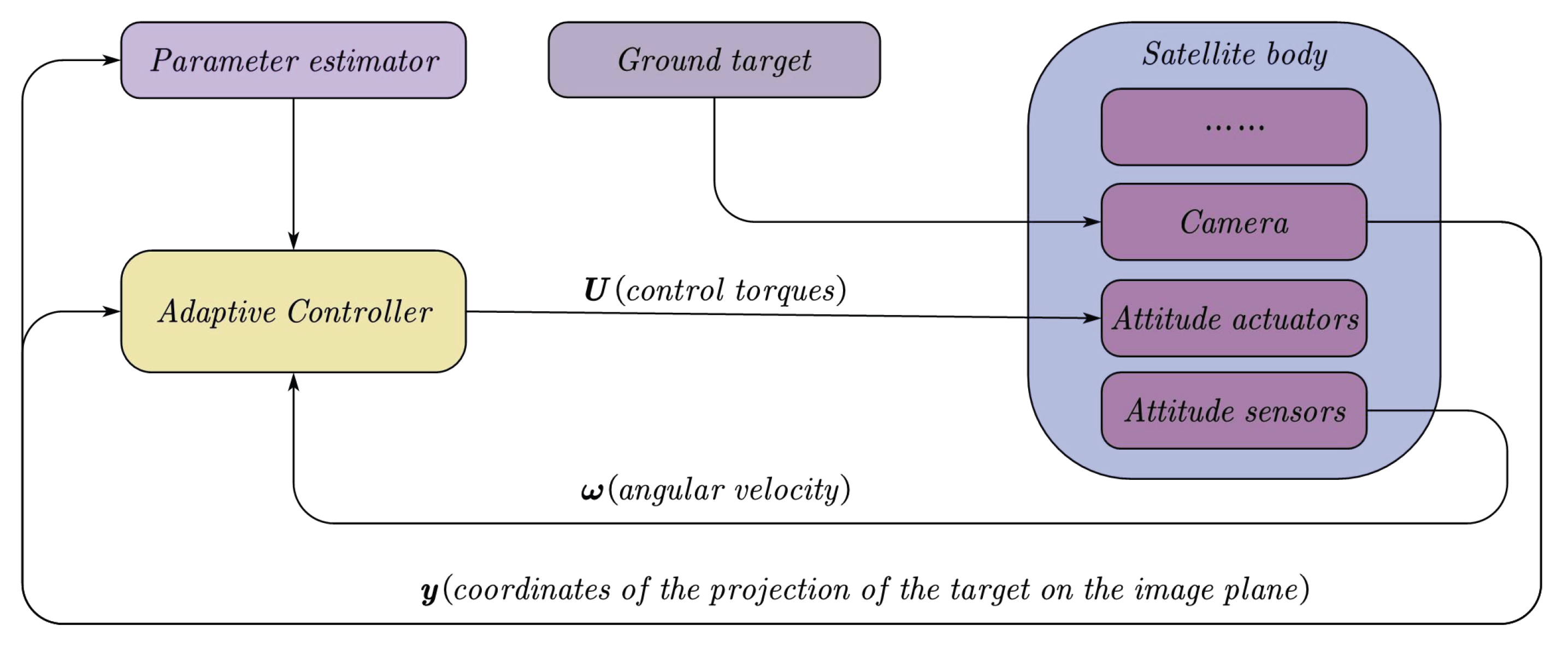
Figure 4 shows the control framework. The camera captures the target when it appears in the field of view, and then the image is processed so that the corresponding target coordinate $\mathit{y}\left(t\right)$ is obtained. With $\mathit{y}\left(t\right)$, the camera parameters are estimated online and are thereafter applied to the attitude controller. According to the kinematics and dynamics, the satellite will finally accomplish the staring attitude maneuver.

3. Controller Design

3.1. Parameter Definition

To analyze the exact parameters that need to be estimated, we rewrite Equation (13) as

$$\begin{array}{cc}\hfill z_c\left(t\right)\left(\begin{array}{c}\mathit{y}\left(t\right)\\ 1\end{array}\right)=& \mathit{N}·T_h\left(t\right)·\left(\begin{array}{c}{}^i{\mathit{R}}_{eT}\left(t\right)\\ 1\end{array}\right)\hfill \\ \hfill =& \mathit{N}·\left(\begin{array}{c}{}^b{\mathit{R}}_{bT}\left(t\right)\\ 1\end{array}\right)\hfill \\ \hfill =& \left(\begin{array}{c}{\mathit{P}}_{\left(3\right)}\\ {\mathit{n}}_{3\left(3\right)}^T\end{array}\right){}^b{\mathit{R}}_{bT}\left(t\right)+\left(\begin{array}{c}{n}_{14}\\ n_{24}\\ n_{34}\end{array}\right)\hfill \end{array}$$

(19)

Comparing the imaging kinematics (16) and (18) with (19), we notice that all the elements in the matrix N can influence projection coordinates, while the projection change rate is only affected by ${\mathit{n}}_{3\left(3\right)}^T$ and ${\mathit{P}}_{\left(3\right)}$. We take all the 12 elements in N as the parameters to be estimated and then form a parameter sequence:

$$\mathit{\theta }={\left(n_{ij}\right)}^{T}i=1,2,3j=1,2,3,4$$

(20)

Theorem 1.

For any $\rho \in \mathbb{R}$ that is not 0, θ and $\rho \mathit{\theta }$ corresponds to the same projection $\mathit{y}\left(t\right)$.

Proof. 

Substitute the depth $z_c\left(t\right)$ in the projection expression in (13) and we have

$$\begin{array}{cc}\hfill \mathit{y}\left(t\right)=& \frac{1}{z_c\left(t\right)}\mathit{P}·T_h\left(t\right)·\left(\begin{array}{c}{}^i{\mathit{R}}_{eT}\left(t\right)\\ 1\end{array}\right)\hfill \\ \hfill =& \frac{\mathit{P}·T_h\left(t\right)·\left(\begin{array}{c}{}^i{\mathit{R}}_{eT}\left(t\right)\\ 1\end{array}\right)}{{\mathit{n}}_3^T·T_h\left(t\right)·\left(\begin{array}{c}{}^i{\mathit{R}}_{eT}\left(t\right)\\ 1\end{array}\right)}\hfill \\ \hfill =& \frac{\rho \mathit{P}·T_h\left(t\right)·\left(\begin{array}{c}{}^i{\mathit{R}}_{eT}\left(t\right)\\ 1\end{array}\right)}{\rho {\mathit{n}}_3^T·T_h\left(t\right)·\left(\begin{array}{c}{}^i{\mathit{R}}_{eT}\left(t\right)\\ 1\end{array}\right)}\hfill \end{array}$$

(21)

It is clear that $\mathit{\theta }$ and $\rho \mathit{\theta }$ result in the same $\mathit{y}\left(t\right)$. A similar property can be obtained for visual servoing application [27]. □

Due to the Theorem 1, the parameters defined in (20) has at least one multiplier difference with the real camera parameters. Without loss of generality, we can force $n_{33}=1$ and only estimate the left parameters in $\mathit{\theta }$, thus the estimation complexities are reduced. We then redefine a new parameter sequence with 11 elements:

$${\mathit{\theta }}_p={\left(n_{11},n_{12},n_{13},n_{14},n_{21},n_{22},n_{23},n_{24},n_{31},n_{32},n_{34}\right)}^T.$$

(22)

Theorem 2.

Assume n represents the number of elements in ${\mathit{\theta }}_p$. For any vector $\mathit{p}\in {\mathbb{R}}^{3\times 1}$ (e.g., the angular velocity ω), the matrices $Y\left(t,\mathit{p}\right)\in {\mathbb{R}}^{2\times n}$, $y\left(t,\mathit{p}\right)\in {\mathbb{R}}^{2\times 1}$, $Z\left(t,\mathit{p}\right)\in {\mathbb{R}}^{1\times n}$, $z\left(t,\mathit{p}\right)\in \mathbb{R}$ can be found, so that the matrices $A\left(t\right)\in {\mathbb{R}}^{2\times 3}$ and $a\left(t\right)\in {\mathbb{R}}^{1\times 3}$ have the following property:

$$\begin{array}{c}\hfill A\left(t,{\mathit{\theta }}_p\right)·\mathit{p}=Y\left(t,\mathit{p}\right)·{\mathit{\theta }}_p+y\left(t,\mathit{p}\right)\\ \hfill a\left(t,{\mathit{\theta }}_p\right)·\mathit{p}=Z\left(t,\mathit{p}\right)·{\mathit{\theta }}_p+z\left(t,\mathit{p}\right)\end{array}$$

(23)

Similarly, the matrices $Y_v^{{}^{\prime }}\left(t\right)\in {\mathbb{R}}^{2\times n}$, $y_v\left(t\right)\in {\mathbb{R}}^{2\times 1}$, $Z_v^{{}^{\prime }}\left(t\right)\in {\mathbb{R}}^{1\times n}$, $z_v\left(t\right)\in \mathbb{R}$ can be found, so that the matrices $A_v\left(t\right)\in {\mathbb{R}}^{2\times 1}$ and $a_v\left(t\right)\in \mathbb{R}$ have the following property:

$$\begin{array}{c}\hfill A_v\left(t,{\mathit{\theta }}_p\right)=Y_v\left(t\right)·{\mathit{\theta }}_p+y_v\left(t\right)\\ \hfill a_v\left(t,{\mathit{\theta }}_p\right)=Z_v\left(t\right)·{\mathit{\theta }}_p+z_v\left(t\right)\end{array}$$

(24)

The proof is omitted here, since it is pretty straightforward based on Equations (15) and (17). Theorem 2 demonstrates that the imaging kinematics can be expressed in a linear form of ${\mathit{\theta }}_p$. This is the basis of the feasibility of estimation. The estimated parameters are denoted as ${\widehat{\mathit{\theta }}}_p\left(t\right)$, where the overhead script$\widehat{}$indicates that the variable is estimated instead of a real value. Correspondingly, this notation applies to all the estimated variables in the remainder of this paper.

3.2. Reference Attitude Trajectory

A PD-like controller requires both the convergence of $\Delta \mathit{y}\left(t\right)$ and the angular velocity error ${\mathit{\omega }}_e\left(t\right)=\mathit{\omega }\left(t\right)-{\mathit{\omega }}_d\left(t\right)$, where ${\mathit{\omega }}_d\left(t\right)$ is the desired angular velocity. ${\mathit{y}}_d$ is predetermined and time-invariant, while ${\mathit{\omega }}_d\left(t\right)$ is time-varying and not as straightforward. Therefore it is troublesome to directly obtain the desired angular velocity trajectory. Instead, a reference attitude trajectory, i.e., ${\mathit{y}}_r\left(t\right)$ and ${\mathit{\omega }}_r\left(t\right)$, is designed to cope with the problem. Define ${\mathit{y}}_r\left(t\right)$ so that it meets the following condition:

$${\dot{\mathit{y}}}_r\left(t\right)={\dot{\mathit{y}}}_d-\lambda \Delta \mathit{y}\left(t\right)=-\lambda \Delta \mathit{y}\left(t\right)$$

(25)

where $\lambda$ is a positive scalar. We further define the reference image tracking error:

$${\mathit{\delta }}_{\dot{\mathit{y}}}\left(t\right)=\dot{\mathit{y}}\left(t\right)-{\dot{\mathit{y}}}_r\left(t\right)=\Delta \dot{\mathit{y}}\left(t\right)+\lambda \Delta \mathit{y}\left(t\right)$$

(26)

Theorem 3.

If ${\mathit{\delta }}_{\dot{\mathit{y}}}\left(t\right)$ asymptotically converges to 0, $\Delta \mathit{y}\left(t\right)$ and $\Delta \dot{\mathit{y}}\left(t\right)$ asymptotically converge to 0; if ${\mathit{\delta }}_{\dot{\mathit{y}}}\left(t\right)$ exponentially converges to 0, $\Delta \mathit{y}\left(t\right)$ and $\Delta \dot{\mathit{y}}\left(t\right)$ exponentially converge to 0;

The theorem is obvious, so no proof is not listed here. Now the control objective is converted to guaranteeing the stability of ${\mathit{\delta }}_{\dot{\mathit{y}}}\left(t\right)$. Meanwhile, the reference angular velocity tracking error is obtained by:

$${\mathit{\delta }}_{\mathit{\omega }}\left(t\right)=\mathit{\omega }\left(t\right)-{\mathit{\omega }}_r\left(t\right)$$

(27)

The reference angular velocity trajectory ${\mathit{\omega }}_r\left(t\right)$ is defined as

$${\mathit{\omega }}_r\left(t\right)={\widehat{A}}^{+}\left(t\right)\left(-{\widehat{z}}_c\left(t\right)·\lambda ·\Delta \mathit{y}\left(t\right)-{\widehat{A}}_v\left(t\right)\right)$$

(28)

where ${\widehat{A}}^{+}\left(t\right)$ is the pseudo-inverse matrix of $\widehat{A}\left(t\right)$, which is the estimated $A\left(t\right)$. ${\widehat{A}}^{+}\left(t\right)$ is defined as

$${\widehat{A}}^{+}\left(t\right)={\widehat{A}}^T\left(t\right){\left[\widehat{A}\left(t\right){\widehat{A}}^T\left(t\right)\right]}^{-1}$$

(29)

The presupposition of the existence of the definition of $\widehat{A}\left(t\right)$ is that $\widehat{A}\left(t\right)$ has a rank of 2. As the values of $\widehat{A}\left(t\right)$ are dependent on ${\widehat{\mathit{\theta }}}_p\left(t\right)$, the rank of $\widehat{A}\left(t\right)$ is affected by the way ${\widehat{\mathit{\theta }}}_p\left(t\right)$ is updated.

3.3. Potential Function Design

Assume the $3\times 3$ sub-matrix of the estimated projection matrix $\widehat{N}\left(t\right)$ is defined as

$${\widehat{N}}_{\left(3\right)}\left(t\right)=\left(\begin{array}{c}{\widehat{\mathit{P}}}_{\left(3\right)}\\ {\widehat{\mathit{n}}}_{3\left(3\right)}^T\end{array}\right)$$

(30)

According to Ref. [28], if ${\widehat{N}}_{\left(3\right)}\left(t\right)$ has a rank of 3, the matrix $\widehat{A}\left(t\right)$ has a rank of 2. Hence, a potential function is designed as

$$U\left({\widehat{\mathit{\theta }}}_p\left(t\right)\right)=\frac{1}{e^{a{\left|{\widehat{N}}_{\left(3\right)}\left(t\right)\right|}^2}-1+b}$$

(31)

Apparently we can conclude that $U\left({\widehat{\mathit{\theta }}}_p\left(t\right)\right)$ is always positive. The coefficients a and b are both positive as well, but b is very small, which is designed to avoid the singular situation where the denominator is 0. The potential function reaches its maximum $\frac{1}{b}$ when $\left|{\widehat{N}}_{\left(3\right)}\left(t\right)\right|=0$, i.e., ${\widehat{N}}_{\left(3\right)}\left(t\right)$ has a rank less than 3. $U\left({\widehat{\mathit{\theta }}}_p\left(t\right)\right)$ will approach to 0 when ${\widehat{\mathit{\theta }}}_p\left(t\right)$ keeps far from the neighborhood of $\left|{\widehat{N}}_{\left(3\right)}\left(t\right)\right|=0$. To ensure that, we should enhance the resistance of ${\widehat{\mathit{\theta }}}_p\left(t\right)$ getting close to the singular area. In the parameter estimation subsection, the self-updating rule will incorporate the gradient of $U\left({\widehat{\mathit{\theta }}}_p\left(t\right)\right)$ regarding ${\widehat{\mathit{\theta }}}_p\left(t\right)$ which is given by

$$\frac{\partial U\left({\widehat{\mathit{\theta }}}_p\left(t\right)\right)}{\partial {\widehat{\mathit{\theta }}}_p\left(t\right)}=-\frac{2a\left|{\widehat{N}}_{\left(3\right)}\left(t\right)\right|e^{a{\left|{\widehat{N}}_{\left(3\right)}\left(t\right)\right|}^2}}{{\left(e^{a{\left|{\widehat{N}}_{\left(3\right)}\left(t\right)\right|}^2}-1+b\right)}^2}\frac{\partial \left|{\widehat{N}}_{\left(3\right)}\left(t\right)\right|}{\partial {\widehat{\mathit{\theta }}}_p\left(t\right)}$$

(32)

3.4. Parameter Estimation

The estimation error is defined as $\Delta {\mathit{\theta }}_p\left(t\right)={\widehat{\mathit{\theta }}}_p\left(t\right)-{\mathit{\theta }}_p$. Equation (11) always holds for an ideal camera whose parameters are all calibrated. However, the real parameters may diverge from the ideal ones. Adopting the definition in [27], we define the following estimated projection errors $\mathit{e}\left(t\right)$ to represent the image deviations caused by $\Delta {\mathit{\theta }}_p$:

$$\mathit{e}\left(t\right)={\widehat{z}}_c\left(t\right)\mathit{y}\left(t\right)-\widehat{\mathit{P}}\left(t\right)T_h\left(t\right)\left(\begin{array}{c}{}^i{\mathit{R}}_{eT}\left(t\right)\\ 1\end{array}\right)$$

(33)

where $\mathit{y}\left(t\right)$ is obtained from the image, and ${\widehat{z}}_c\left(t\right)$ and $\widehat{P}\left(t\right)$ are the estimated depth and parameters.

Theorem 4.

Given the estimated projection errors $\mathit{e}\left(t\right)$, there exists a matrix $W_p\left(t\right)\in R^{2\times n}$, so that

$$\mathit{e}\left(t\right)=W_p\left(t\right)\Delta {\mathit{\theta }}_p\left(t\right)$$

(34)

Proof. 

According to the projection Equation (11), with the real parameters we have

$$z_c\left(t\right)\mathit{y}\left(t\right)-\mathit{P}·T_h\left(t\right)\left(\begin{array}{c}{}^i{\mathit{R}}_{eT}\left(t\right)\\ 1\end{array}\right)=0$$

(35)

Thus, $\mathit{e}\left(t\right)$ can be rewritten as

$$\begin{array}{cc}\hfill \mathit{e}\left(t\right)=& {\widehat{z}}_c\left(t\right)\mathit{y}\left(t\right)-\widehat{\mathit{P}}\left(t\right)T_h\left(t\right)\left(\begin{array}{c}{}^i{\mathit{R}}_{eT}\left(t\right)\\ 1\end{array}\right)-\left(z_c\left(t\right)\mathit{y}\left(t\right)-\mathit{P}·T_h\left(t\right)\left(\begin{array}{c}{}^i{\mathit{R}}_{eT}\left(t\right)\\ 1\end{array}\right)\right)\hfill \\ \hfill =& \left({\widehat{z}}_c\left(t\right)-z_c\left(t\right)\right)\mathit{y}\left(t\right)-\left(\widehat{\mathit{P}}\left(t\right)-\mathit{P}\right)T_h\left(t\right)\left(\begin{array}{c}{}^i{\mathit{R}}_{eT}\left(t\right)\\ 1\end{array}\right)\hfill \\ \hfill =& \mathit{y}\left(t\right)\left({\widehat{\mathit{n}}}_3^T\left(t\right)-{\mathit{n}}_3^T\right)T_h\left(t\right)\left(\begin{array}{c}{}^i{\mathit{R}}_{eT}\left(t\right)\\ 1\end{array}\right)-\left(\widehat{\mathit{P}}\left(t\right)-\mathit{P}\right)T_h\left(t\right)\left(\begin{array}{c}{}^i{\mathit{R}}_{eT}\left(t\right)\\ 1\end{array}\right)\hfill \\ \hfill =& \left[\mathit{y}\left(t\right)\left({\widehat{\mathit{n}}}_3^T\left(t\right)-{\mathit{n}}_3^T\right)-\left(\widehat{\mathit{P}}\left(t\right)-\mathit{P}\right)\right]T_h\left(t\right)\left(\begin{array}{c}{}^i{\mathit{R}}_{eT}\left(t\right)\\ 1\end{array}\right)\hfill \end{array}$$

(36)

$\left({\widehat{\mathit{n}}}_3^T\left(t\right)-{\mathit{n}}_3^T\right)$ and $\left(\widehat{\mathit{P}}\left(t\right)-\mathit{P}\right)$ appear linearly in the last equation, such that $\Delta \mathit{\theta }\left(t\right)$ can be linearized from $\mathit{e}\left(t\right)$. Considering that $n_{33}$ and ${\widehat{n}}_{33}$ in $\mathit{\theta }$ and $\widehat{\mathit{\theta }}$ are both fixed to 1, we can eliminate $n_{33}-{\widehat{n}}_{33}$ in Equation (36). Then we can conclude that $\mathit{e}\left(t\right)$ is linear with respect to $\Delta {\mathit{\theta }}_p\left(t\right)$, i.e., such a matrix $W_p\left(t\right)$ exists. Apparently, $W_p\left(t\right)$ consists of $\mathit{y}\left(t\right)$, $T_h\left(t\right)$ and ${}^i{\mathit{R}}_{eT}\left(t\right)$. □

We propose the following self-updating rule for the parameters:

$${\dot{\widehat{\mathit{\theta }}}}_p\left(t\right)=-{\Gamma }^{-1}\left\{{\mathit{Y}}_p^T\left(t\right){\mathit{\delta }}_{\dot{\mathit{y}}}\left(t\right)+W_p^T\left(t\right)K_1\mathit{e}\left(t\right)+K_2\frac{\partial U\left({\widehat{\mathit{\theta }}}_p\left(t\right)\right)}{\partial {\widehat{\mathit{\theta }}}_p\left(t\right)}{∥{\mathit{\delta }}_{\mathit{\omega }}\left(t\right)∥}^2\right\}$$

(37)

$\Gamma$, $K_1$, $K_2$ and $K_3$ are all positive coefficient matrices, and ${\mathit{Y}}_p^T\left(t\right)$ is a regressor matrix which does not contain any camera parameters. It is defined via the following equation:

$$\Delta {\mathit{\theta }}_p^T\left(t\right)·{\mathit{Y}}_p^T\left(t\right)=-{\left[\left(z_c\left(t\right)-{\widehat{z}}_c\left(t\right)\right){\dot{\mathit{y}}}_r\left(t\right)-\left(A_v\left(t\right)-{\widehat{A}}_v\left(t\right)\right)-\left(A\left(t\right)-\widehat{A}\left(t\right)\right)\mathit{\omega }\left(t\right)\right]}^T{K}_3$$

(38)

There are three components in the brace of Equation (37). The first one is about the reference image tracking error, which will play a part in the stability proof. The second is about the negative gradient of the estimated projection error, which drives down $\mathit{e}\left(t\right)$ by updating ${\widehat{\mathit{\theta }}}_p\left(t\right)$. Additionally, the last term is the negative gradient of the potential function, which mainly takes effect when ${\widehat{\mathit{\theta }}}_p\left(t\right)$ is approaching an area that leads to $rank\left(\widehat{A}\left(t\right)\right)<2$.

3.5. Adaptive Staring Imaging Controller

The controller is given by

$$\mathit{U}\left(t\right)=\mathit{\omega }\left(t\right)\times J\mathit{\omega }\left(t\right)+J{\dot{\mathit{\omega }}}_r\left(t\right)-K_4{\mathit{\delta }}_{\mathit{\omega }}\left(t\right)-{\widehat{A}}^T\left(t\right)K_3{\mathit{\delta }}_{\dot{\mathit{y}}}\left(t\right)-K_5∥\frac{\partial U\left({\widehat{\mathit{\theta }}}_p\left(t\right)\right)}{\partial {\widehat{\mathit{\theta }}}_p\left(t\right)}∥{\mathit{\delta }}_{\mathit{\omega }}\left(t\right)$$

(39)

where $K_4$ and $K_5$ are positive coefficient matrices. For simplicity, we define 2 non-negative functions:

$$\begin{array}{cc}\hfill V_1\left(t\right)=& \frac{1}{2}{\mathit{\delta }}_{\mathit{\omega }}^T\left(t\right)J{\mathit{\delta }}_{\mathit{\omega }}\left(t\right)\hfill \\ \hfill V_2\left(t\right)=& \frac{1}{2}\Delta {\mathit{\theta }}_p^T\left(t\right)\Gamma \Delta {\mathit{\theta }}_p\left(t\right)\hfill \end{array}$$

(40)

The derivatives of $V_1\left(t\right)$ and $V_2\left(t\right)$ are given respectively as follows

$$\begin{array}{cc}\hfill {\dot{V}}_1\left(t\right)=& {\mathit{\delta }}_{\mathit{\omega }}^T\left(t\right)J{\dot{\mathit{\delta }}}_{\mathit{\omega }}\left(t\right)\hfill \\ \hfill =& {\mathit{\delta }}_{\mathit{\omega }}^T\left(t\right)J\left(\dot{\mathit{\omega }}\left(t\right)-{\dot{\mathit{\omega }}}_r\left(t\right)\right)\hfill \\ \hfill =& {\mathit{\delta }}_{\mathit{\omega }}^T\left(t\right)\left(-\mathit{\omega }\left(t\right)\times J\mathit{\omega }\left(t\right)+\mathit{U}\left(t\right)-J{\dot{\mathit{\omega }}}_r\left(t\right)\right)\hfill \\ \hfill =& {\mathit{\delta }}_{\mathit{\omega }}^T\left(t\right)\left(-K_4{\mathit{\delta }}_{\mathit{\omega }}\left(t\right)-{\widehat{A}}^T\left(t\right)K_3{\mathit{\delta }}_{\dot{\mathit{y}}}\left(t\right)-K_5∥\frac{\partial U\left({\widehat{\mathit{\theta }}}_p\left(t\right)\right)}{\partial {\widehat{\mathit{\theta }}}_p\left(t\right)}∥{\mathit{\delta }}_{\mathit{\omega }}\left(t\right)\right)\hfill \\ \hfill =& -{\mathit{\delta }}_{\mathit{\omega }}^T\left(t\right)K_4{\mathit{\delta }}_{\mathit{\omega }}\left(t\right)-{\mathit{\delta }}_{\mathit{\omega }}^T\left(t\right){\widehat{A}}^T\left(t\right)K_3{\mathit{\delta }}_{\dot{\mathit{y}}}\left(t\right)-K_5{\mathit{\delta }}_{\mathit{\omega }}^T\left(t\right)∥\frac{\partial U\left({\widehat{\mathit{\theta }}}_p\left(t\right)\right)}{\partial {\widehat{\mathit{\theta }}}_p\left(t\right)}∥{\mathit{\delta }}_{\mathit{\omega }}\left(t\right)\hfill \end{array}$$

(41)

$$\begin{array}{cc}\hfill {\dot{V}}_2\left(t\right)=& \Delta {\mathit{\theta }}_p^T\left(t\right)\Gamma \Delta {\dot{\mathit{\theta }}}_p\left(t\right)\hfill \\ \hfill =& -\Delta {\mathit{\theta }}_p^T\left(t\right)\left\{{\mathit{Y}}_p^T\left(t\right){\mathit{\delta }}_{\dot{\mathit{y}}}\left(t\right)+W_p^T\left(t\right)K_1\mathit{e}\left(t\right)+K_2\frac{\partial U\left({\widehat{\mathit{\theta }}}_p\left(t\right)\right)}{\partial {\widehat{\mathit{\theta }}}_p\left(t\right)}{∥{\mathit{\delta }}_{\mathit{\omega }}\left(t\right)∥}^2\right\}\hfill \\ \hfill =& -\Delta {\mathit{\theta }}_p^T\left(t\right){\mathit{Y}}_p^T\left(t\right){\mathit{\delta }}_{\dot{\mathit{y}}}\left(t\right)-{\mathit{e}}^T\left(t\right)K_1\mathit{e}\left(t\right)-\Delta {\mathit{\theta }}_p^T\left(t\right)K_2\frac{\partial U\left({\widehat{\mathit{\theta }}}_p\left(t\right)\right)}{\partial {\widehat{\mathit{\theta }}}_p\left(t\right)}{∥{\mathit{\delta }}_{\mathit{\omega }}\left(t\right)∥}^2\hfill \end{array}$$

(42)

The ${\mathit{\delta }}_{\mathit{\omega }}^T\left(t\right){\widehat{A}}^T\left(t\right)K_3{\mathit{\delta }}_{\dot{\mathit{y}}}\left(t\right)$ in the expression of ${\dot{V}}_1\left(t\right)$ can be decomposed into ${\mathit{\omega }}^T\left(t\right){\widehat{A}}^T\left(t\right)K_3{\mathit{\delta }}_{\dot{\mathit{y}}}\left(t\right)$ and $-{\mathit{\omega }}_r^T\left(t\right){\widehat{A}}^T\left(t\right)K_3{\mathit{\delta }}_{\dot{\mathit{y}}}\left(t\right)$. We have

$$\begin{array}{cc}\hfill {\mathit{\omega }}^T\left(t\right){\widehat{A}}^T\left(t\right)=& {\mathit{\omega }}^T\left(t\right)A^T\left(t\right)+{\mathit{\omega }}^T\left(t\right)\left({\widehat{A}}^T\left(t\right)-A^T\left(t\right)\right)\hfill \\ \hfill =& {\left[z_c\left(t\right)\dot{\mathit{y}}\left(t\right)-A_v\left(t\right)\right]}^T+{\mathit{\omega }}^T\left(t\right)\left({\widehat{A}}^T\left(t\right)-A^T\left(t\right)\right)\hfill \\ \hfill =& {\left[z_c\left(t\right){\dot{\mathit{y}}}_r\left(t\right)+z_c\left(t\right)\left(\dot{\mathit{y}}\left(t\right)-{\dot{\mathit{y}}}_r\left(t\right)\right)-A_v\left(t\right)\right]}^T+{\mathit{\omega }}^T\left(t\right)\left({\widehat{A}}^T\left(t\right)-A^T\left(t\right)\right)\hfill \\ \hfill =& {\left[z_c\left(t\right){\dot{\mathit{y}}}_r\left(t\right)-A_v\left(t\right)+z_c\left(t\right){\mathit{\delta }}_{\dot{\mathit{y}}}\left(t\right)\right]}^T+{\mathit{\omega }}^T\left(t\right)\left({\widehat{A}}^T\left(t\right)-A^T\left(t\right)\right)\hfill \\ \hfill {\mathit{\omega }}_r^T\left(t\right){\widehat{A}}^T\left(t\right)=& {\left[{\widehat{z}}_c\left(t\right){\dot{\mathit{y}}}_r\left(t\right)-{\widehat{A}}_v\left(t\right)\right]}^T\hfill \end{array}$$

(43)

Thus with the definition of ${\mathit{Y}}_p^T\left(t\right)$ in Equation (38), ${\mathit{\delta }}_{\mathit{\omega }}^T\left(t\right){\widehat{A}}^T\left(t\right)K_3{\mathit{\delta }}_{\dot{\mathit{y}}}\left(t\right)$ is decomposed into

$$\begin{array}{cc}\hfill & {\mathit{\delta }}_{\mathit{\omega }}^T\left(t\right){\widehat{A}}^T\left(t\right)K_3{\mathit{\delta }}_{\dot{\mathit{y}}}\left(t\right)={\left(\mathit{\omega }\left(t\right)-{\mathit{\omega }}_r\left(t\right)\right)}^T{\widehat{A}}^T\left(t\right)K_3{\mathit{\delta }}_{\dot{\mathit{y}}}\left(t\right)\hfill \\ \hfill =& {\left[\left(z_c\left(t\right)-{\widehat{z}}_c\left(t\right)\right){\dot{\mathit{y}}}_r\left(t\right)-\left(A_v\left(t\right)-{\widehat{A}}_v\left(t\right)\right)+\left(\widehat{A}\left(t\right)-A\left(t\right)\right)\mathit{\omega }\left(t\right)+z_c\left(t\right){\mathit{\delta }}_{\dot{\mathit{y}}}\left(t\right)\right]}^T{K}_3{\mathit{\delta }}_{\dot{\mathit{y}}}\left(t\right)\hfill \\ \hfill =& z_c\left(t\right){\mathit{\delta }}_{\dot{\mathit{y}}}\left(t\right)K_3{\mathit{\delta }}_{\dot{\mathit{y}}}\left(t\right)+\hfill \\ & {\left[\left(z_c\left(t\right)-{\widehat{z}}_c\left(t\right)\right){\dot{\mathit{y}}}_r\left(t\right)-\left(A_v\left(t\right)-{\widehat{A}}_v\left(t\right)\right)+\left(\widehat{A}\left(t\right)-A\left(t\right)\right)\mathit{\omega }\left(t\right)\right]}^T{K}_3{\mathit{\delta }}_{\dot{\mathit{y}}}\left(t\right)\hfill \\ \hfill =& z_c\left(t\right){\mathit{\delta }}_{\dot{\mathit{y}}}\left(t\right)K_3{\mathit{\delta }}_{\dot{\mathit{y}}}\left(t\right)-\Delta {\mathit{\theta }}_p^T\left(t\right){\mathit{Y}}_p^T\left(t\right){\mathit{\delta }}_{\dot{\mathit{y}}}\left(t\right)\hfill \end{array}$$

(44)

Now we define the Lyapunov function $V\left(t\right)=V_1\left(t\right)+V_2\left(t\right)$. Substitute Equation (44) into Equation (41) and we obtain the derivative of $V\left(t\right))$:

$$\begin{array}{cc}\hfill \dot{V}\left(t\right)=& {\dot{V}}_1\left(t\right)+{\dot{V}}_2\left(t\right)\hfill \\ \hfill =& -{\mathit{\delta }}_{\mathit{\omega }}^T\left(t\right)K_4{\mathit{\delta }}_{\mathit{\omega }}\left(t\right)-z_c\left(t\right){\mathit{\delta }}_{\dot{\mathit{y}}}\left(t\right)K_3{\mathit{\delta }}_{\dot{\mathit{y}}}\left(t\right)-{\mathit{e}}^T\left(t\right)K_1\mathit{e}\left(t\right)\hfill \\ \hfill & -K_5{\mathit{\delta }}_{\mathit{\omega }}^T\left(t\right)∥\frac{\partial U\left({\widehat{\mathit{\theta }}}_p\left(t\right)\right)}{\partial {\widehat{\mathit{\theta }}}_p\left(t\right)}∥{\mathit{\delta }}_{\mathit{\omega }}\left(t\right)-\Delta {\mathit{\theta }}_p^T\left(t\right)K_2\frac{\partial U\left({\widehat{\mathit{\theta }}}_p\left(t\right)\right)}{\partial {\widehat{\mathit{\theta }}}_p\left(t\right)}{∥{\mathit{\delta }}_{\mathit{\omega }}\left(t\right)∥}^2\hfill \\ \hfill ⩽& -{\mathit{\delta }}_{\mathit{\omega }}^T\left(t\right)K_4{\mathit{\delta }}_{\mathit{\omega }}\left(t\right)-z_c\left(t\right){\mathit{\delta }}_{\dot{\mathit{y}}}\left(t\right)K_3{\mathit{\delta }}_{\dot{\mathit{y}}}\left(t\right)-{\mathit{e}}^T\left(t\right)K_1\mathit{e}\left(t\right)\hfill \\ \hfill & -\left(K_5-∥\Delta {\mathit{\theta }}_p^T\left(t\right)∥K_2\right)∥\frac{\partial U\left({\widehat{\mathit{\theta }}}_p\left(t\right)\right)}{\partial {\widehat{\mathit{\theta }}}_p\left(t\right)}∥{∥{\mathit{\delta }}_{\mathit{\omega }}\left(t\right)∥}^2\hfill \end{array}$$

(45)

Assume $k_{5min}$ is the smallest eigenvalue of $K_5$, $k_{2max}$ is the biggest eigenvalue of $K_2$, and ${\tau }_{min}$ is the smallest eigenvalue of $\Gamma$. Select proper values so that

$$k_{5min}⩾k_{2max}\sqrt{\frac{2V\left(0\right)}{{\tau }_{min}}}$$

(46)

In this way, we can guarantee

$$\dot{V}\left(t\right)⩽0$$

(47)

According to Equations (45) and (47), $V\left(t\right)$ is bounded and the upper bound is $V\left(0\right)$. Taking the expression of $V\left(t\right)$ from (40) into account, $\mathit{\omega }\left(t\right)$, ${\mathit{\omega }}_r\left(t\right)$ and ${\widehat{\mathit{\theta }}}_p\left(t\right)$ are all bounded variables. Due to the definition of ${\mathit{\omega }}_r\left(t\right)$ and ${\mathit{y}}_r\left(t\right)$, the boundedness of ${\mathit{\omega }}_r\left(t\right)$ implies that the boundedness of $\mathit{y}\left(t\right)$ and ${\mathit{y}}_r\left(t\right)$. The bounded ${\widehat{\mathit{\theta }}}_p\left(t\right)$ also indicates the estimated projection error $\mathit{e}\left(t\right)$ is bounded, as is obvious in Equation (34). Attributing to the boundedness of the aforementioned variables, we can infer that $\ddot{V}\left(t\right)$ is also bounded. According to Barbalat’s Lemma, we can conclude that

$$\underset{t\to \infty }{lim}\dot{V}\left(t\right)=0$$

(48)

i.e.,

$$\begin{array}{cc}\hfill \underset{t\to \infty }{lim}{\mathit{\delta }}_{\mathit{\omega }}\left(t\right)& =\mathbf{0}\hfill \\ \hfill \underset{t\to \infty }{lim}{\mathit{\delta }}_{\dot{\mathit{y}}}\left(t\right)& =\mathbf{0}\hfill \\ \hfill \underset{t\to \infty }{lim}\mathit{e}\left(t\right)& =\mathbf{0}\hfill \end{array}$$

(49)

As Theorem 3 suggests, we have

$$\begin{array}{c}\hfill \underset{t\to \infty }{lim}\Delta \mathit{y}\left(t\right)=\mathbf{0}\\ \hfill \underset{t\to \infty }{lim}\Delta \dot{\mathit{y}}\left(t\right)=\mathbf{0}\end{array}$$

(50)

Hence, the stability of the proposed adaptive staring imaging controller (37) and (39) is proved. Although the camera is uncalibrated, the estimated projection error $\mathit{e}\left(t\right)$ is defined to help to estimate the parameters. As the parameters are updated online, the controller utilizes the image extraction information $\mathit{y}\left(t\right)$ and angular velocity $\mathit{\omega }\left(t\right)$ as the input and then computes the errors between the input and the reference trajectory. The control torques will finally direct the projection of the target point to its desired location on the image plane and achieve staring observation.

4. Simulation and Discussion

In this section, the proposed image-based adaptive staring controller and a conventional position-based controller are applied to realize the ground target observation.

At the initial time (12 Jul 2021 04:30:00.000 UTC), the ground target’s location is given in

Table 1. Ground target location.

Longitude (${}^{\circ }$)	Latitude Values (${}^{\circ }$)	Height (km)
128.271	64.72	0

and the orbital elements of the satellite are listed in

Table 2. Orbital elements.

Semimajor Axis (km)	Eccentricity	Inclination (${}^{\circ }$)	Argument of Perigee (${}^{\circ }$)	Right Ascension of the Ascending Node (${}^{\circ }$)	True Anomaly (${}^{\circ }$)
6868.14	0	97.2574	59.3884	290.017	54.8163

. The target is initially near the sub-satellite point. The real and theoretical camera parameters are listed in

Table 3. Camera parameters.

Camera Parameters	Theoretical Values	Real Values
f	1 m	1.1 m
$u_0$	376	396
$v_0$	291	276
$dx$	$8.33\times {10}^{-6}$ m	$8.43\times {10}^{-6}$
$dy$	$8.33\times {10}^{-6}$ m	$8.43\times {10}^{-6}$
${}^c{\mathit{R}}_{bc}$	$\left(\begin{array}{c}-0.2682\\ 0.0408\\ 0.0671\end{array}\right)$m	$\left(\begin{array}{c}-0.2582\\ 0.0358\\ 0.0771\end{array}\right)$m
${}_b{}^{c}M$	$M_{321}\left(-{30}^{\circ },{40}^{\circ },-{20}^{\circ }\right)$	$M_{321}\left(-{29}^{\circ },39.6^{\circ },-18.9^{\circ }\right)$

. $M_{321}\left(·\right)$ denotes the rotation matrix with a 3-2-1 rotation sequence. The theoretical parameters were initially real states of the camera and are used as the initial estimated values. Due to various causes, e.g., the long-term oscillation, the real parameters deviate from the theoretical ones and reflect the current camera states. The image plane of the camera consists of $752\times 582$ pixels. The desired projection location is at the center of the plane, i.e., ${(u_0,v_0)}^T$. The initial attitude is presented in

Table 4. Initial attitude.

Quaternion	Angular Velocity (${}^{\circ }/\mathit{s}$)
${(0.4228,0.6600,0.5414,-0.3040)}^T$	${(0.0178,0.0587,-0.0167)}^T$

where the camera is roughly kept pointing to Earth center.

In the given initial conditions, the ground target already appears on the image. The control torques are bounded by the maximum output $U_{max}$ of the attitude actuator, i.e., a reaction flywheel, which in our simulation is $0.1$ Nm. So the inequality $∥U_i\left(t\right)∥⩽U_{max}$ holds for $i=1,2,3$. The following two cases are simulated using the same uncalibrated camera and the same initial attitude and orbit conditions. In case 1, the conventional position-based controller only utilizes target’s location information without taking advantage of the images. In case 2, we suppose the image processing algorithm detects its pixel coordinates and the image-based adaptive controller outputs the control torques incorporating the image and location information.

4.1. Case 1: Conventional Position-based Staring Controller

The conventional staring control methods are normally based on the location of the ground target. By designing the desired orientation and angular velocity, the optical axis of camera is supposed to be aimed at the target in an ideally calibrated camera case. Using the uncalibrated camera and the initial conditions presented in this section, we adopt a position-based staring controller from [2]. The controller is

$$\begin{array}{c}\hfill \mathit{U}\left(t\right)=K_{\delta }\mathit{\delta }-K_{\omega }\Delta \mathit{\omega }\end{array}$$

(51)

where $K_{\delta }$ and $K_{\omega }$ are the coefficient matrices. Let $\mathit{\delta }={(\alpha ,\beta )}^T$ where $\alpha$ and $\beta$ are the two rotation angles between the camera’s optical axis and its desired orientation aiming at the target. Let $\Delta \mathit{\omega }=\mathit{\omega }-{\mathit{\omega }}_d$ where ${\mathit{\omega }}_d$ is the desired angular velocity. $\alpha$, $\beta$ and ${\mathit{\omega }}_d$ are designed based on target’s position. Refer to the original article for more detailed definitions.

Table 5. Position-based control parameters.

${\mathit{K}}_{\mathit{\delta }}$	${\mathit{K}}_{\mathit{\omega }}$
$\left(\begin{array}{cc}4& 0\\ 0& 1.6\\ 0& 0\end{array}\right)$	$\left(\begin{array}{ccc}2.5& 0& 0\\ 0& 2.5& 0\\ 0& 0& 2.5\end{array}\right)$

shows the coefficient values adopted in the simulation.

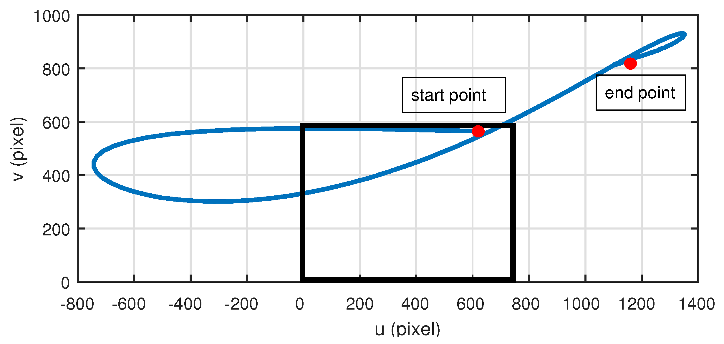
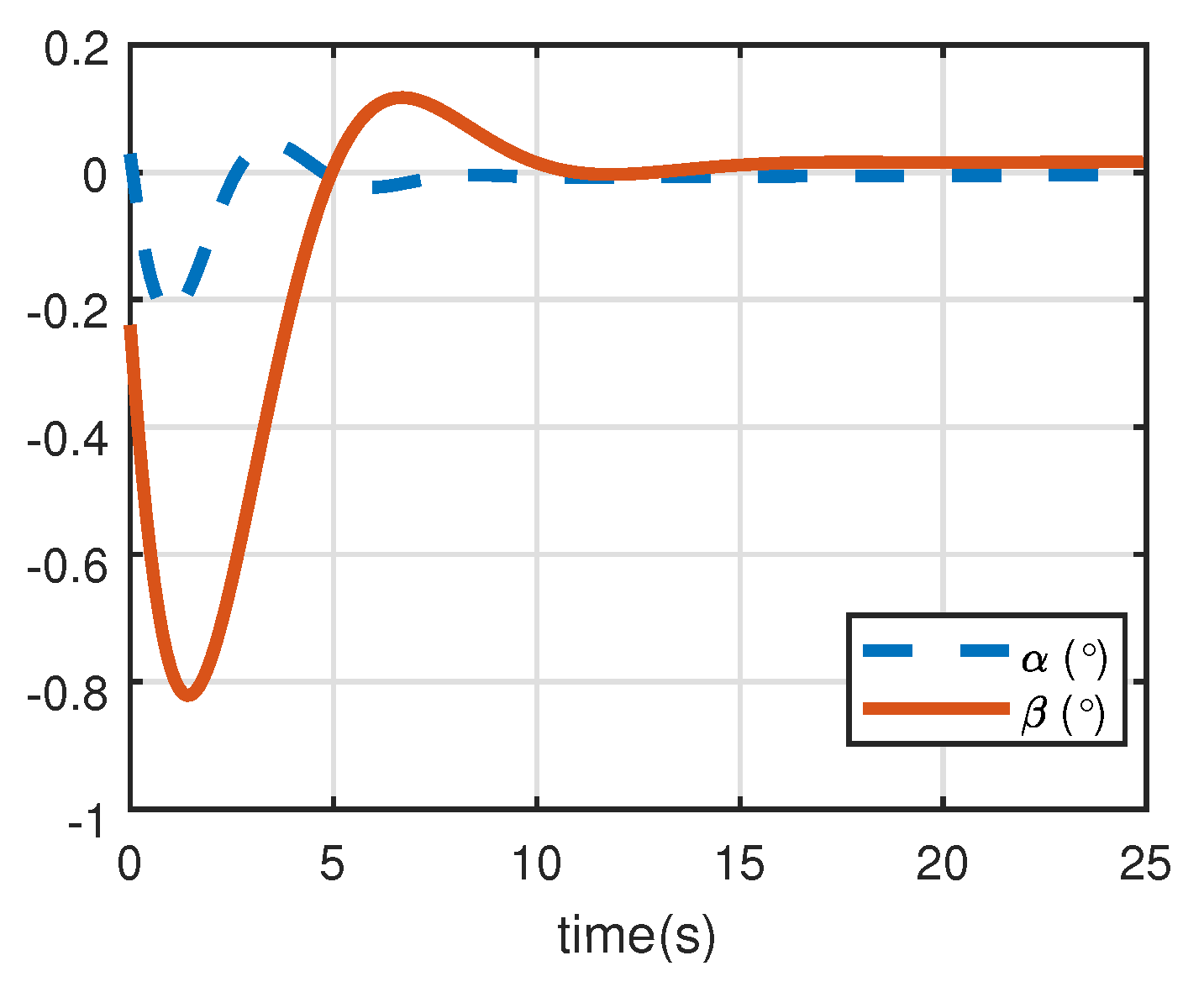
The target’s trajectory on the image plane is shown in Figure 5 where the black box is the field of view. Figure 6 depicts the changes of two rotation angles. The initial location of the ground point is the upper right corner of the plane marked by the start point. As the controller starts working, the target gradually moves out of the field of view, which means the camera can not see the target temporarily. Since this controller is dependent on the position, it can still work without the sight. However, the end point shown in the Figure 5 demonstrates that when the satellite finishes attitude maneuvering and is at the stable staring stage, the target is still lost in our image. This leads to the failure of observing the ground target, which results from the uncalibrated camera. According to transform matrix from the body frame to camera frame ${}_b{}^{c}M$ in Table 3, the optical axis of camera has over $1^{\circ }$ deviation from its ideal orientation in the body frame. Hence, when the position-based controller thinks the optical axis is aimed at the target, the target is actually lost in the view.

4.2. Case 2: Image-Based Adaptive Staring Controller

Table 6. Image-based control parameters.

Control Parameters	Values
$K_1$	${10}^{-15}\times E_2$
$K_2$	${10}^{-3}$
$K_3$	$2.5\times {10}^{-15}\times E_2$
$K_4$	$2\times E_3$
$K_5$	$30\times E_3$
$\Gamma$	$\mathrm{diag}\left\{8\times {10}^{-4}\times E_8,1000\times E_3\right\}$
a	1
b	0.001

shows the control coefficients in the controller. The operation $\mathrm{diag}\left\{·\right\}$ represents a matrix with the elements located at the diagonal consecutively.

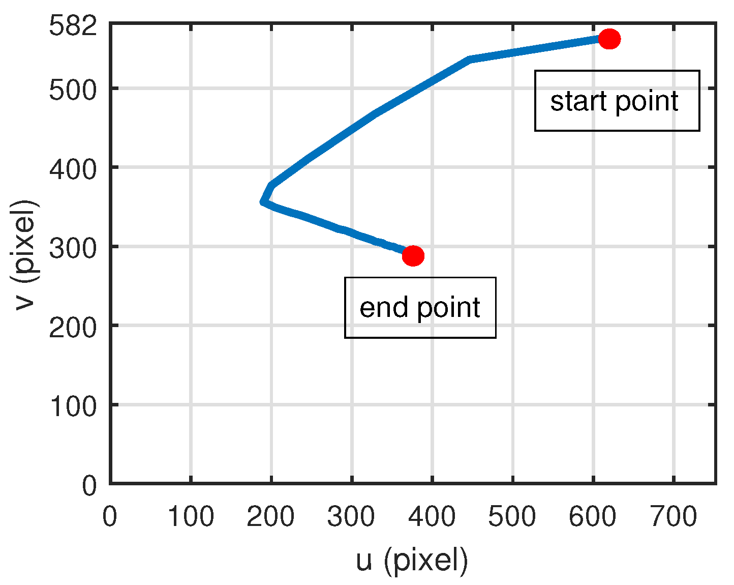
Figure 7 depicts the trace of the target’s projection on the image plane. Initially, the target appears at the same location on the image plane as in the case Section 4.1. With the staring controller working properly, the projection moves along the trajectory and finally reaches the end point, which is also the image center $(376,291)$. The trajectory indicates that it takes some time for the controller to find the proper direction of the desired destination, because the initial guess of the parameters is primary factor affecting the accuracy of the controller at the starting stage. Furthermore, the initial angular velocity of the satellite also determines the initial moving direction the target. 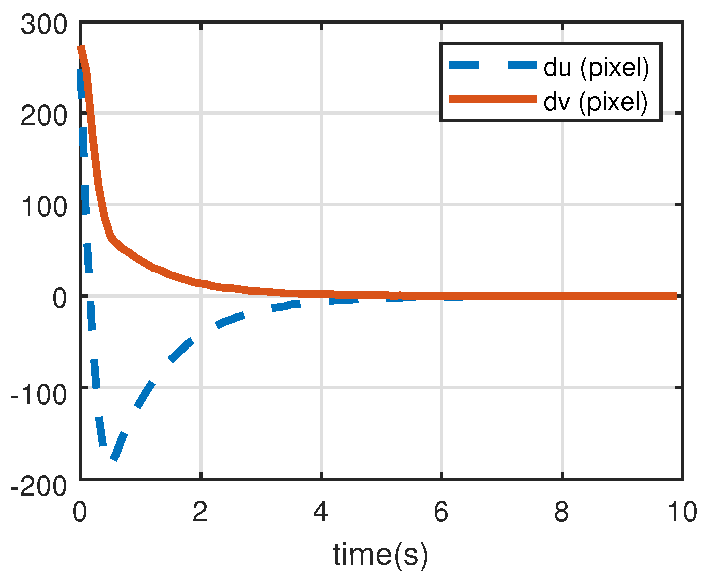Figure 8 shows the differences between the current and the desired coordinates and it reflects the same trend as Figure 7.

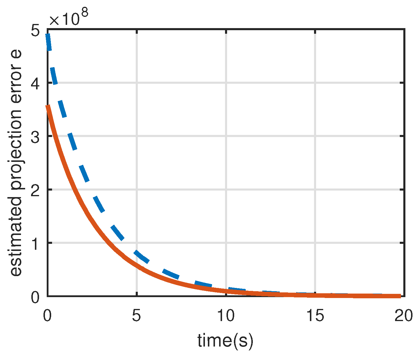
Figure 9 is the time evolution of estimated projection errors. The adaptive rule continuously updates the parameters in the negative gradient direction of $\mathit{e}\left(t\right)$, so the estimated projection errors can be reduced due to the parameter estimation.

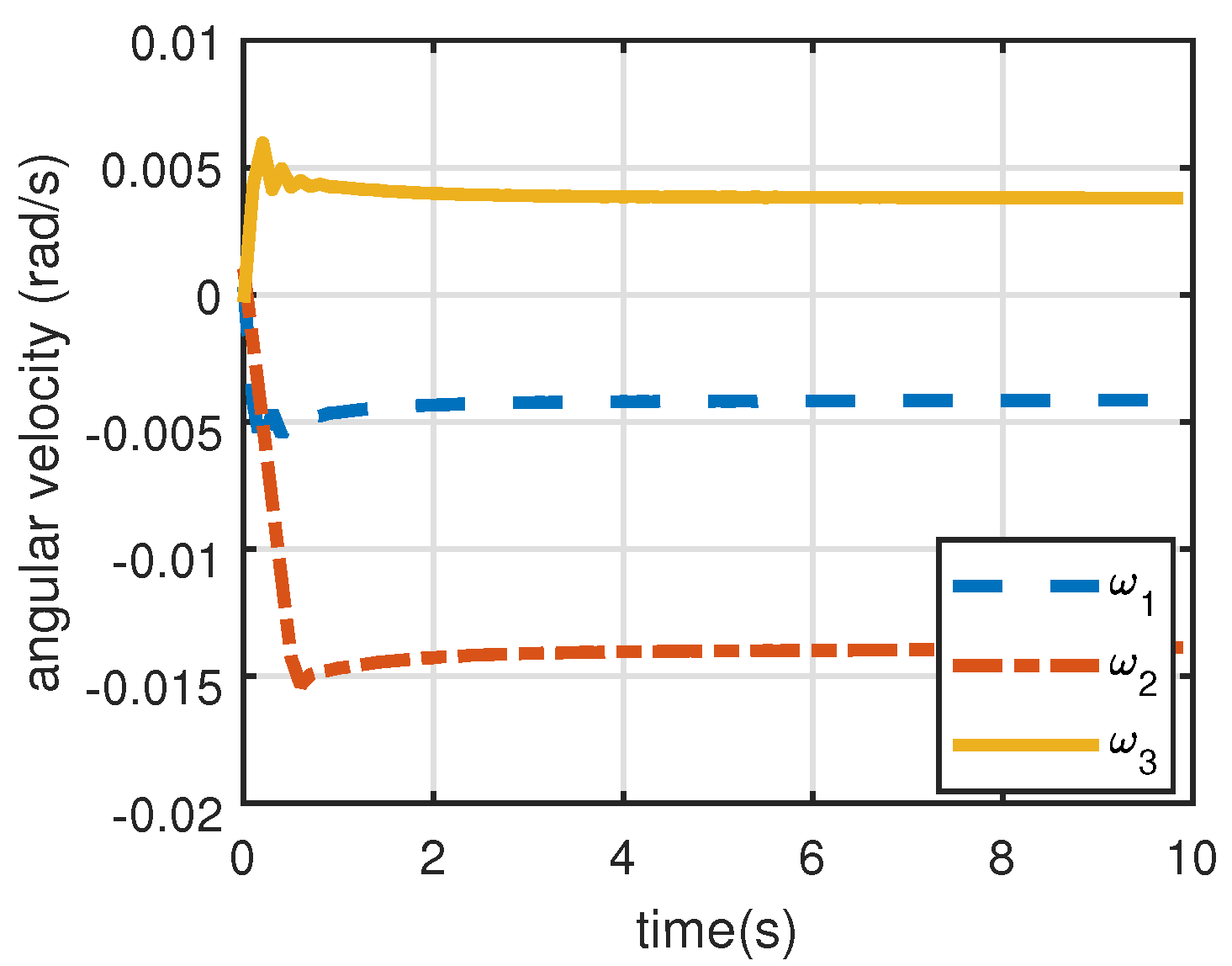
Figure 10 shows the angular velocities of the satellite. At first, $\mathit{\omega }\left(t\right)$ adjusts very fast and is then gradually stabilized. It is worth noting that $\mathit{\omega }\left(t\right)$ is not convergent to $\mathbf{0}$, because the ground target is a moving point in the inertial space. The satellite is required to rotate at a certain rate to keep staring at it. Moreover, from Figure 10 we can see that the final angular velocity is not a constant but varies at a very low speed because of the relative motion between the ground point and the satellite. 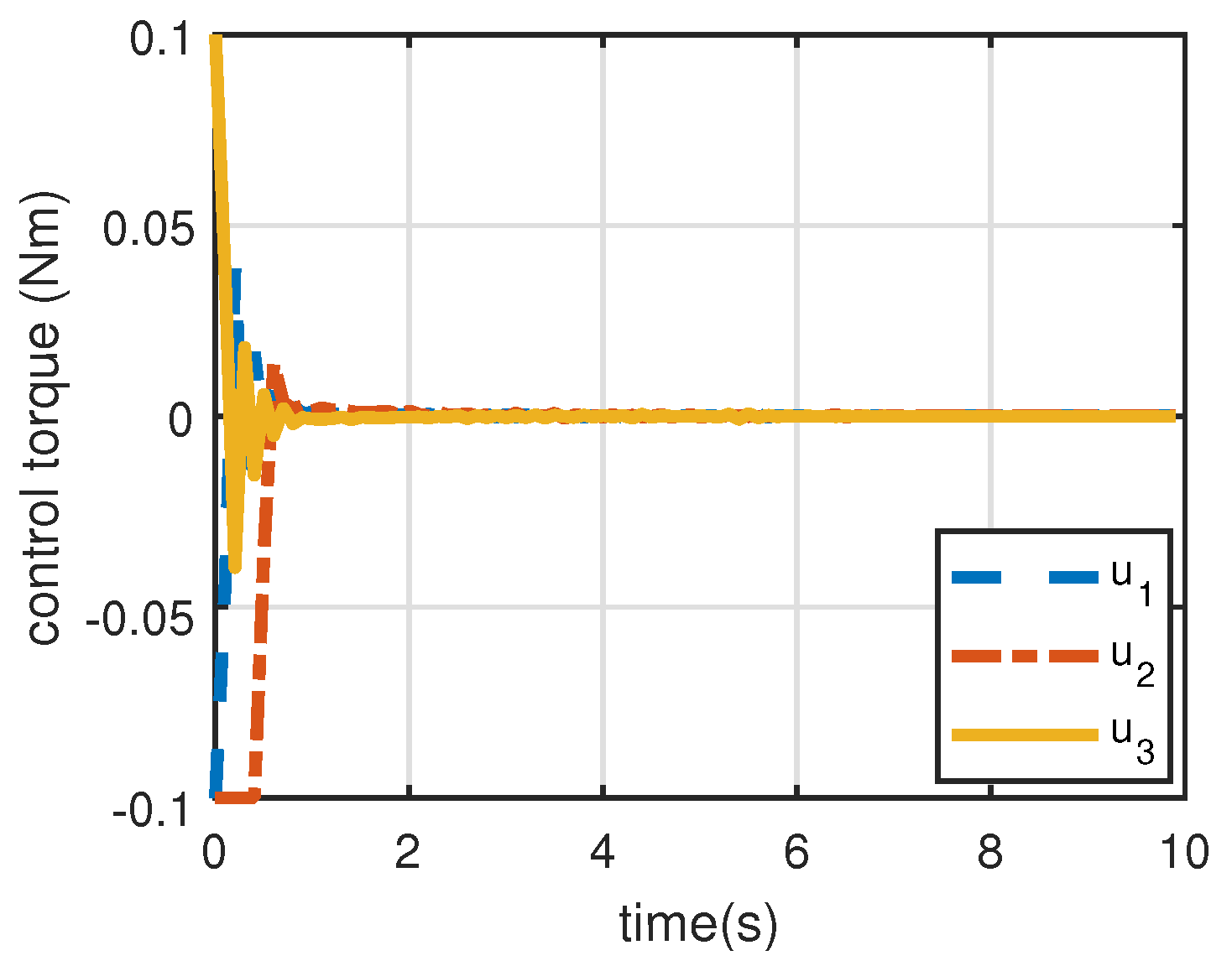Figure 11 shows the control torques generated by attitude actuators. In the starting process, $u_2$ reaches its upper bound which is the joint result of the parameter estimation, the initial image errors and the initial angular velocity. As the target projection approaches its desired location, the control torques are decreasing and are eventually kept within a narrow range to meet the need for the aforementioned minor adjustment of the angular acceleration.

Here, we sum up these two cases. For a position-based staring controller, it fails at coping with the deviation in the presence of an uncalibrated camera. For the proposed image-based adaptive staring controller, although the camera parameters are not unknown, the online estimation can reduce the estimated projection errors. With this technique, control torques are generated to drive the target projection to its desired location. The simulation demonstrates that the adaptive controller achieves the goal of keeping the target’s projection at the center and we can expect that high precision can be realized to gain better ground target staring observation. Only small control torques are needed to maintain the constant tracking in the stable staring process.

5. Conclusions and Outlook

For a video satellite, staring attitude control has been its main working mode and has reaped many promising applications. This paper proposes an adaptive controller that takes the camera’s model into account. First, the projection kinematics are established based on the staring imaging scenario, where constant relative motion exists. Second, an attitude reference trajectory is introduced to avoid designing the desired angular velocity and a potential function is introduced to guarantee that the definition of the reference angular velocity exists. Third, we define the parameters that need to be estimated and a corresponding parameter updating rule is proposed. Finally, the image and attitude information is incorporated to form the adaptive staring controller, which is constructed using the estimated variables. Stability is proved and the projection is successfully controlled to the predetermined desired location on the image plane in the simulation. Thus, an image-based staring controller for an uncalibrated camera is formulated.

While we can obtain the information of ground targets, it is hard to predict the motion of many moving targets such as planes and ships. In the further study, non-cooperative targets should be dealt with where the relative motion is unknown.

References

1. Zhang, X.Y.; Xiang, J.H. Tracking imaging feedback attitude control of video satellite. In Proceedings of the ELECTRICAL ENGINEERING AND AUTOMATION: Proceedings of the International Conference on Electrical Engineering and Automation (EEA2016), Hong Kong, China, 24–26 June 2016; World Scientific: Singapore, 2017; pp. 729–737. [Google Scholar]
2. Lian, Y.; Gao, Y.; Zeng, G. Staring imaging attitude control of small satellites. J. Guid. Control Dyn. 2017, 40, 1278–1285. [Google Scholar] [CrossRef]
3. Buhl, M.; Segert, T.; Danziger, B. TUBSAT—A Reliable and Cost Effective Micro Satellite Platform. In Proceedings of the 61st International Astronautical Congress, International Astronautical Federation Paper IAC-10-B4, Prague, Czech Republic, 27 September–1 October 2010; Volume 6. [Google Scholar]
4. Luo, Y.; Zhou, L.; Wang, S.; Wang, Z. Video satellite imagery super resolution via convolutional neural networks. IEEE Geosci. Remote Sens. Lett. 2017, 14, 2398–2402. [Google Scholar] [CrossRef]
5. Xiao, A.; Wang, Z.; Wang, L.; Ren, Y. Super-resolution for “Jilin-1” satellite video imagery via a convolutional network. Sensors 2018, 18, 1194. [Google Scholar] [CrossRef] [PubMed] [Green Version]
6. Jiang, K.; Wang, Z.; Yi, P.; Jiang, J. A progressively enhanced network for video satellite imagery superresolution. IEEE Signal Process. Lett. 2018, 25, 1630–1634. [Google Scholar] [CrossRef]
7. Chen, X.; Ma, Y.; Geng, Y.; Feng, W.; Dong, Y. Staring imaging attitude tracking control of agile small satellite. In Proceedings of the 2011 6th IEEE Conference on Industrial Electronics and Applications, Beijing, China, 21–23 June 2011; pp. 143–148. [Google Scholar]
8. Geng, Y.; Li, C.; Guo, Y.; Biggs, J.D. Hybrid robust and optimal control for pointing a staring-mode spacecraft. Aerosp. Sci. Technol. 2020, 105, 105959. [Google Scholar] [CrossRef]
9. Li, C.; Geng, Y.; Guo, Y.; Han, P. Suboptimal Repointing Maneuver of a staring-mode spacecraft with one DOF for final attitude. Acta Astronaut. 2020, 175, 349–361. [Google Scholar] [CrossRef]
10. Cui, K.; Xiang, J.; Zhang, Y. Mission planning optimization of video satellite for ground multi-object staring imaging. Adv. Space Res. 2018, 61, 1476–1489. [Google Scholar] [CrossRef]
11. Li, P.; Dong, Y.; Li, H. Staring Imaging Real-Time Optimal Control Based on Neural Network. Int. J. Aerosp. Eng. 2020, 2020, 8822223. [Google Scholar] [CrossRef]
12. Zhang, X.; Xiang, J. Moving object detection in video satellite image based on deep learning. In Proceedings of the LIDAR Imaging Detection and Target Recognition 2017. International Society for Optics and Photonics, Changchun, China, 23–25 July 2017; Volume 10605, p. 106054H. [Google Scholar]
13. Zhang, X.; Xiang, J.; Zhang, Y. Space object detection in video satellite images using motion information. Int. J. Aerosp. Eng. 2017, 2017, 1024529. [Google Scholar] [CrossRef] [Green Version]
14. Yan, Z.; Song, X.; Zhong, H.; Jiang, F. Moving object detection for video satellite based on transfer learning deep convolutional neural networks. In Proceedings of the 10th International Conference on Pattern Recognition Systems (ICPRS-2019), Tours, France, 8–10 July 2019; pp. 106–111. [Google Scholar]
15. Yu, S.; Yuanbo, Y.; He, X.; Lu, M.; Wang, P.; An, X.; Fang, X. On-Board Fast and Intelligent Perception of Ships With the “Jilin-1” Spectrum 01/02 Satellites. IEEE Access 2020, 8, 48005–48014. [Google Scholar] [CrossRef]
16. Zhao, X.; Emami, M.R.; Zhang, S. Robust image-based control for spacecraft uncooperative rendezvous and synchronization using a zooming camera. Acta Astronaut. 2021, 184, 128–141. [Google Scholar] [CrossRef]
17. Zhang, H.; Jiang, Z.; Elgammal, A. Vision-based pose estimation for cooperative space objects. Acta Astronaut. 2013, 91, 115–122. [Google Scholar] [CrossRef]
18. Huang, Y.; Zhu, M.; Zheng, Z.; Low, K.H. Linear velocity-free visual servoing control for unmanned helicopter landing on a ship with visibility constraint. IEEE Trans. Syst. Man Cybern. Syst. 2021, 52, 2979–2993. [Google Scholar] [CrossRef]
19. Shirzadeh, M.; Asl, H.J.; Amirkhani, A.; Jalali, A.A. Vision-based control of a quadrotor utilizing artificial neural networks for tracking of moving targets. Eng. Appl. Artif. Intell. 2017, 58, 34–48. [Google Scholar] [CrossRef]
20. Jabbari Asl, H.; Yoon, J. Robust image-based control of the quadrotor unmanned aerial vehicle. Nonlinear Dyn. 2016, 85, 2035–2048. [Google Scholar] [CrossRef]
21. Prabowo, Y.A.; Trilaksono, B.R.; Triputra, F.R. Hardware in-the-loop simulation for visual servoing of fixed wing UAV. In Proceedings of the 2015 international conference on electrical engineering and informatics (ICEEI), Denpasar, Indonesia, 10–11 August 2015; pp. 247–252. [Google Scholar]
22. Zheng, D.; Wang, H.; Wang, J.; Zhang, X.; Chen, W. Toward visibility guaranteed visual servoing control of quadrotor UAVs. IEEE/ASME Trans. Mechatron. 2019, 24, 1087–1095. [Google Scholar] [CrossRef]
23. Liang, X.; Wang, H.; Liu, Y.H.; Chen, W.; Jing, Z. Image-based position control of mobile robots with a completely unknown fixed camera. IEEE Trans. Autom. Control 2018, 63, 3016–3023. [Google Scholar] [CrossRef]
24. Xu, F.; Wang, H.; Liu, Z.; Chen, W. Adaptive visual servoing for an underwater soft robot considering refraction effects. IEEE Trans. Ind. Electron. 2019, 67, 10575–10586. [Google Scholar] [CrossRef]
25. Xie, H.; Low, K.H.; He, Z. Adaptive visual servoing of unmanned aerial vehicles in GPS-denied environments. IEEE/ASME Trans. Mechatron. 2017, 22, 2554–2563. [Google Scholar] [CrossRef]
26. Felicetti, L.; Emami, M.R. Image-based attitude maneuvers for space debris tracking. Aerosp. Sci. Technol. 2018, 76, 58–71. [Google Scholar] [CrossRef]
27. Wang, H.; Liu, Y.H.; Zhou, D. Adaptive visual servoing using point and line features with an uncalibrated eye-in-hand camera. IEEE Trans. Robot. 2008, 24, 843–857. [Google Scholar] [CrossRef]
28. Wang, H.; Liu, Y.H.; Chen, W. Uncalibrated visual tracking control without visual velocity. IEEE Trans. Control. Syst. Technol. 2010, 18, 1359–1370. [Google Scholar] [CrossRef]
Figure 1. The ground-target-staring observation geometry.
Aerospace 09 00283 g001
Figure 2. The intrinsic camera model.
Aerospace 09 00283 g002
Figure 3. The extrinsic camera model.
Aerospace 09 00283 g003
Figure 4. The framework of the image-based staring control.
Aerospace 09 00283 g004
Figure 5. The projection trajectory on the image plane for the position-based controller.
Aerospace 09 00283 g005
Figure 6. The evolution of rotation angles α and β .
Aerospace 09 00283 g006
Figure 7. The projection trajectory on the image plane.
Aerospace 09 00283 g007
Figure 8. The evolution of image errors.
Aerospace 09 00283 g008
Figure 9. The evolution of estimated projection error.
Aerospace 09 00283 g009
Figure 10. The evolution of angular velocities.
Aerospace 09 00283 g010
Figure 11. The evolution of control torques.
Aerospace 09 00283 g011