Track Segment Association Method Based on Bidirectional Track Prediction and Fuzzy Analysis

Abstract

Due to sensor characteristics, geographical environment, electromagnetic interference, electromagnetic silence, information countermeasures, and other reasons, the phenomenon of track breakages occur in the process of aircraft track data processing. It leads to the change in target label attributes. In order to make the track segment association effect better, we studied several existing time series prediction methods, and proposed a track segment association method based on bidirectional Holt-Winters prediction and fuzzy analysis. This algorithm bidirectionally predicts and extrapolates track segments by the Holt-Winters method, and then uses the fuzzy track segment association algorithm to perform segment association and secondary association. The simulation results of this method show that the track segment association method based on Holt-Winters prediction and fuzzy analysis can effectively solve the track association problem where the target label attributes change before and after track breakage, demonstrating better association ability and robustness. Compared with the fuzzy association method without adding track prediction, our method generally improves the association accuracy by 35%.

1. Introduction

The aircraft tracks generally have the characteristics of high density, high velocity, low relative speed between targets and poor separability. Affected by sensor characteristics, geographical environment, electromagnetic interference, electromagnetic silence, information confrontation, and other uncertain factors, the track data will be interrupted, leading to the change in target label attributes, and severely undermining information fusion. Track breakage leads the computer to re-batch and re-track the targets, thus increasing the tracking burden of devices, and reducing the efficiency of tracking measurement. Solving the problem of track segment association before and after track breakage of the same target can not only improve the continuity and stability of target tracking, but also provide strong support for follow-up tracking, strikes, and other related tasks.

The track segment association problems can be divided into the track association problems based on discrete points and continuous time tracks according to whether it is continuous. The problem based on discrete points is to regard the track as discrete track points and judge whether the track is correlated through two segments of track points. The continuous track association models the trajectory of the target movement through an engineering-friendly, time trajectory function (T-FoT), and then the smoothing and tracking problem becomes the estimation/fitting T-FoT problem [1,2,3,4,5].

In 1971, R. A. Singer and others proposed and developed the nearest neighbor method [6], which is a tracking method with fixed memory and can work in a multi-echo environment. It is mainly suitable for high signal-to-noise ratio and small target density. condition. In 1972, Y. Bar-Shalom proposed the probabilistic data association method (PDA) [7]. The advantage of this algorithm is that the probability of mistracking and losing the target is small and the calculation amount is small when tracking a single target in a clutter environment. In order to adapt to the dense multi-target tracking environment, Y. Bar-Shalom proposed a joint probabilistic data association algorithm (JPDA) [8] on the basis of PDA. This method defines joint events and introduces the concept of “cluster”, by calculating the joint probability of joint events, the edge probability of the association between the echo and the target is calculated. In 1974, R. A. Singer and R. G. Sea et al. developed a class of “full-neighbor” filters [9] that not only consider all candidate callbacks, but also the tracking history. After that, D. B. Reid proposed a statistical decision-based multiple hypothesis method (MHT) [10] for data association based on the “full-neighbor” filter and Y. Bar-Shalom’s clustering matrix concept. The algorithm mainly includes the generation of aggregation, the generation of “hypothesis”, the calculation of “hypothesis” probability, and the process of hypothesis reduction. The advantage of the algorithm is that the effect is better, and the disadvantage is that it relies too much on the prior knowledge of the target and clutter. After the development of the MHT algorithm, the trajectory-oriented MHT algorithm emerged. The trajectory is initialized, updated, and the score is calculated before it is stored in the hypothesis. The process of calculating the score includes comparing the probability of the correct target trajectory and the probability of the wrong target set. The score function [11,12] used to calculate the score can score the trajectory points, and then judge whether it is a reasonable trajectory according to the score. Impossible trajectories are removed before trajectories are combined into hypotheses. In 2001, D. Schultz et al. proposed a data association algorithm based on particle filtering and joint probabilistic data association [13]. Particle filtering is based on a large number of measurements, through the evolution and propagation of a set of weighted particles to recursively approximate the posterior probability density function of the state, so as to obtain other statistics about the state. This method has broad development space in the field of data association based on nonlinear models. In addition, Y. Bar-Shalom and J. K. Tugnait et al. [14] proposed a multi-maneuvering target tracking algorithm combining IMM and JPDA. At the same time, Y. Bar-Shalom and X. R. Li, etc. [14], proposed a multi-maneuvering target tracking algorithm combining IMM and MHT.

The abovementioned traditional algorithms have the characteristics of a large amount of calculations and high requirements for the prior information of target maneuvering, so they are not suitable for long-term tracking environments with concentrated targets and have poor robustness. As the tracking environment becomes more and more complex, the algorithm will inevitably move in the direction of a suitable calculation amount and less requirement for target prior information. In recent years, a large number of scholars have introduced intelligent algorithms such as neural networks and fuzzy theory into existing association algorithms to make up for the shortcomings of high requirements for target prior information.

The track segment association method based on Holt-Winters prediction and fuzzy analysis can better solve these problems. First of all, thanks to the first prediction and then the association in the algorithm, it can bring a better association effect than the traditional method. Secondly, due to the low complexity of the algorithm, the algorithm executes faster than the neural network. The final algorithm basically requires no prior information. The experimental results show that the algorithm proposed in this paper can achieve long-term high-precision correlation.

In general, to solve the problem of track data discontinuity in track data processing with changed track label attributes after breakage and for long breakage periods, we propose a TSA method based on Holt-Winters prediction and fuzzy analysis that can effectively associate track segments before and after track breakage. In this method, eigenvectors are input into the Holt-Winters model to complete the prediction and bidirectionally extrapolation of track data, and then the fuzzy track association algorithm is employed to perform track segment association and secondary association.

2. Materials and Methods

The core idea of the algorithm in this paper is to transform the TSA problem into a problem of first performing track prediction and then performing track segment association by using methods based on the fuzzy factors on direction, acceleration, and unified velocity, making association strategies and automatically adjusting the association threshold of the membership function. In the present work, the first part introduces relevant theories of the Holt-Winters method, the second part explains the fuzzy track association algorithm, and the last part presents the structure and process of this new algorithm.

2.1. Holt-Winters Method

This part introduces the Holt-Winters method, serving as a basis for further track prediction and track association.

The Holt-Winters method [15,16,17,18,19,20] is a time series analysis and prediction method. It is suitable for the non-stationary series with linear trends and periodic fluctuations. The exponential moving average (EMA) method is used to make the model parameters adapt to the changes in the non-stationary series and to make short-term forecasts for future trends. The Holt-Winters method, adding the Winters period term (also called season term) based on the Holt model, is applicable to deal with the fluctuation of fixed periods or cycles in time series such as monthly data (period 12), quarterly data (period 4), and weekly data (period 7). Adding multiple Winters terms can also help deal with the coexistence of multiple cycles.

The Holt-Winters method, suitable for non-stationary series with linear trends and fixed cycles, contains additive and multiplicative models. In the additive model, or additive seasonality model, it is assumed that the trend component $u_t$ and the seasonal component $s_t$ of the time series $x_t$ have an additive relationship, namely, $x_t=u_t+s_t$ in the ideal case, where $u_t$ increases (or decreases) linearly with time, and $s_t$ is the seasonal component of period T. In practice, due to the non-stationarity of the time series $x_t$, the linear increasing rate of the trend component $u_t$ and the seasonal component $s_t$ are relatively fixed in the short term, but can change gradually over the long run. In addition, $x_t$ may contain the irregular noise component. Therefore, we need to employ the EMA method to continuously calibrate the $u_t$ and $s_t$ components in the model according to the actual observations $x_t$. The formulas are as follows:

$$\begin{array}{l}{u}_t=\alpha \times \left(X_t-S_t-T\right)+(1-\alpha )\times \left(u_{t-1}+v_{t-1}\right)\\ v_t=\beta \times \left(u_t-u_{t-1}\right)+(1-\beta )\times v_{t-1}\\ s_t=\gamma \times \left(x_t-u_t\right)+(1-\gamma )\times s_{t-T}\end{array}$$

(1)

in the above three equations, there are three smoothing parameters $\alpha$, $\beta$ and $\gamma$, all between 0 and 1. They are the balanced weight between the prediction results and the actual extrapolation results. $v_t$ represents the linear increasing rate of the trend component $u_t$. The larger the parameters $\alpha$, $\beta$ and $\gamma$ are, the stronger the non-stationarity of the time series $x_t$ is, and the shorter the predictable time of the model is, so it is necessary to adjust the components of the model more quickly. On the contrary, if smaller parameters $\alpha$, $\beta$ and $\gamma$ can be used to match the historical data, the consistency between the model and data is better and the predictable time will be longer.

As the historical data are used up and the model enters the prediction stage from the training stage, let $\alpha =\beta =\gamma =0$, there is no more data to modify the model, the prediction result of $x_t$ can be calculated with the formula $x_t=u_t+s_t$ in the ideal situation. In order to determine the reasonable parameters $\alpha$, $\beta$ and $\gamma$ and the predictable time, we can try to use cross validation to deal with it. The historical data are divided into two sections. The first section is used to train the model. After the first section of date is used up, the model will enter the prediction stage, and then the prediction results will be compared with the second section of historical data.

For the multiplicative model, or the multiplicative seasonality model, it is assumed that the trend component $u_t$ and the seasonal component $s_t$ have a multiplicative relationship, namely, $x_t=u_t\times s_t$ in the ideal situation. The training method for this model is similar to that for the additive model. The formulas are as follows:

$$\begin{array}{l}{u}_t=\alpha \times \left(x_t/s_{t-T}\right)+(1-\alpha )\times \left(u_{t-1}+v_{t-1}\right)\\ v_t=\beta \times \left(u_t-u_{t-1}\right)+(1-\beta )\times v_{t-1}\\ s_t=\gamma \times \left(x_t/u_t\right)+(1-\gamma )\times s_{t-T}\end{array}$$

(2)

when carrying out prediction, let $\alpha =\beta =\gamma =0$, and calculate the prediction result according to $x_t=u_t\times s_t$. As a nonlinear model, the multiplicative model can deal with the change in the amplitude of seasonal fluctuation with the trend component, so it depends more on a good initial value than the additive model. Generally, the data within the first cycle T of $x_t$ is are intercepted and become the initial waveform of $s_1,s_2,\dots ,s_t$ after detrending and denoising. The additive model is a linear model and can be written in the form of matrix in the training and prediction stages for the convenience of analyzing its numerical stability. However, both models require a fixed period $l$ in the periodic component $s_t$.

2.2. Fuzzy Track Association Algorithm

In order to calculate the similarity of two tracks, the corresponding sets of fuzzy factors, fuzzy factor weights, and membership functions need to be determined. Let $U=\{u_1,u_2,\cdots ,u_k,\cdots ,u_n\}$ be the fuzzy factor set, where $u_k$ is the k-th fuzzy factor that affects the decision. Fuzzy factors fall into three categories. The first is one-dimensional information, which mainly refers to the Euclidean distance based on target positions, speeds, headings, and heading change rates. The second is two-dimensional information, which is mainly about the Euclidean distance based on target positions, velocities, and accelerations along the x-axis and y-axis of the target, and the Euclidean distance based on the headings and the heading change rates. The third is three-dimensional information, including the Euclidean distance based on target positions, velocities, accelerations, direction cosine angles, and cosine angle change rates of the target along the x, y, and z axes. According to practical experience, the position factor of the target is the primary factor in determining whether the trajectory is relevant, whether it is speed or heading will eventually lead to the change in the target position; the secondary factors that determine whether the trajectory is relevant are the speed and heading factors, because they change rapidly, so not suitable as a determinant for judging whether trajectories are relevant. In practical calculation, the most important factor is the target location factor in the fuzzy factor set, so the weight of this factor should be set to the maximum. The influence of the speed factor is relatively small, and it is given the second largest weight. The heading factor has the least influence, so its weight is set to be very small or zero. According to the above principles, we have the fuzzy factor weight set $A=(a_1,a_2,\cdots ,a_k,\cdots ,a_n)$, where $a_k$ represents the weight corresponding to the k-th factor $u_k$, and generally ${\displaystyle {\sum }_{k=1}^n{a}_k}=1$. Considering the characteristics of the sensor, there is $a_1\ge a_2\ge a_3\ge \cdots \ge a_n$. To get the $u_k$(k = 1,2,…,n), it is necessary to establish the set of fuzzy factors between tracks according to the state estimation vectors ${\widehat{X}}_i(t/t)$ and ${\widehat{X}}_j(t/t)$ and it is assumed that $\widehat{X}\left(t/t\right)=\left[\widehat{x}\left(t\right),\widehat{y}\left(t\right),\widehat{z}\left(t\right),\widehat{\dot{x}}\left(t\right),\widehat{\dot{y}}\left(t\right),\widehat{\dot{z}}\left(t\right),\widehat{\ddot{x}}\left(t\right),\widehat{\ddot{y}}\left(t\right),\widehat{\ddot{z}}\left(t\right)\right]$.

Therefore, the initial values of fuzzy factors and weight vectors can be determined for state estimation according to three different situations. The membership function is the core of fuzzy theory that solves the problem of track association. According to the characteristics of fuzzy factors in track association, available membership functions include normal distribution, Cauchy distribution, centralized distribution gamma distribution, etc. After determining the fuzzy factor set, fuzzy factor weight set, and deviation spread, the normal membership function is used to calculate the association degree of the two targets as follows:

$$f_{ij}\left(t\right)={\displaystyle \sum }_{k=1}^n{a}_k\left(t\right){\mu }_k;i\in U_1,j\in U_2$$

(3)

where $f_{ij}$ represents the association degree of the two targets $i$ and $j$ at the t-th moment, which is the sum of the products of the $k$ membership degrees ${\mu }_1$, ${\mu }_2$, ${\mu }_3$ and the corresponding weights $a_1,a_2,a_3$ at the t-th moment. For n tracks and m tracks of target 1 and target 2, a fuzzy association matrix at the t-th moment can be constructed:

$$F\left(t\right)=\left(\begin{array}{cccc}{f}_{11}\left(t\right)& f_{12}\left(t\right)& \cdots & f_{1m}\left(t\right)\\ f_{21}\left(t\right)& f_{22}\left(t\right)& \cdots & f_{2m}\left(t\right)\\ \cdots & \cdots & \cdots & \cdots \\ f_{n1}\left(t\right)& f_{n2}\left(t\right)& \cdots & f_{nm}\left(t\right)\end{array}\right)$$

(4)

where the largest element $f_{ij}(t)$ is found in $F(t)$. For a certain threshold $\epsilon$, if $f_{ij}(t)>\epsilon$, then $i$ and $j$ targets are associated, otherwise they are not.

2.3. Fuzzy Track Segment Association Algorithm

To deal with the change in the target label attributes after track breakage, we first comprehensively consider the velocity, azimuth, acceleration, breakage period, and other factors of the high-velocity and highly maneuvering targets and perform multi-level association. Then, we take the threshold as a function of the breakage period $l$, and combine it with the breakage period factor to judge the association, so as to solve the problem that the deviation increases with the extension of the breakage period. When determining the fuzzy factor set, it is necessary to calculate the corresponding Euclidean distance between target positions, velocities, courses, and course change rates. For air targets under different conditions, we should consider velocity factors, direction factors, acceleration, and other fuzzy factors comprehensively, which are expressed as:

$$\{\begin{array}{l}{u}_1\left(t\right)={[{({\widehat{x}}_i\left(t\right)-{\widehat{x}}_j\left(t\right))}_2+{({\widehat{y}}_i\left(t\right)-{\widehat{y}}_j\left(t\right))}_2+{({\widehat{z}}_i\left(t\right)-{\widehat{z}}_j\left(t\right))}_2]}^{0.5}\\ u_2\left(t\right)={[{({\widehat{\dot{x}}}_i\left(t\right)-{\widehat{\dot{x}}}_j\left(t\right))}_2+{({\widehat{\dot{y}}}_i\left(t\right)-{\widehat{\dot{y}}}_j\left(t\right))}_2+{({\widehat{\dot{z}}}_i\left(t\right)-{\widehat{\dot{z}}}_j\left(t\right))}_2]}^{0.5}\\ u_3\left(t\right)={[{({\widehat{\ddot{x}}}_i\left(t\right)-{\widehat{\ddot{x}}}_j\left(t\right))}_2+{({\widehat{\ddot{y}}}_i\left(t\right)-{\widehat{\ddot{y}}}_j\left(t\right))}_2+{({\widehat{\ddot{z}}}_i\left(t\right)-{\widehat{\ddot{z}}}_j\left(t\right))}_2]}^{0.5}\end{array}$$

(5)

where $u_1$, $u_2$ and $u_3$ represent the fuzzy factors on position, velocity, and acceleration, respectively. For air targets, considering the relationship between velocity and direction, we directly subtract the velocities on each axis, and then combine the velocity and direction to form a fuzzy factor. In this paper, the normal membership function is used for track association:

$${\mu }_k\left(u_k\right)=\exp \left[-{\tau }_k\left(u_k^2/{\sigma }_k^2\right)\right]$$

(6)

where $u_k$ is the k-th fuzzy factor in the fuzzy factor set, ${\sigma }_k$ is the spread of the k-th fuzzy factor, and ${\tau }_k$ is the adjustment degree. When there is system deviation, it will greatly influence the fuzzy factors on position, velocity, and acceleration. In the fuzzy factor set, the spread of the position, velocity, and acceleration factors should be adjusted accordingly. The membership function is expressed as:

$$\{\begin{array}{c}{\mu }_1\left(u_1\right)=\exp \left[-{\tau }_1\left(\frac{u_1^2}{{\sigma }_x^2+{\sigma }_y^2+{\sigma }_z^2}\right)\right]\\ {\mu }_2\left(u_2\right)=\exp \left[-{\tau }_2\left(\frac{u_2^2}{{\sigma }_{\dot{x}}^2+{\sigma }_{\dot{y}}^2+{\sigma }_{\dot{z}}^2}\right)\right]\\ {\mu }_3\left(u_3\right)=\exp \left[-{\tau }_3\left(\frac{u_3^2}{{\sigma }_{\ddot{x}}^2+{\sigma }_{\ddot{y}}^2+{\sigma }_{\ddot{z}}^2}\right)\right]\end{array}$$

(7)

where ${\sigma }_x$, ${\sigma }_y$ and ${\sigma }_z$ represent the spread of the fuzzy factor on position, namely, the position error variance; ${\sigma }_{\dot{x}}$, ${\sigma }_{\dot{y}}$ and ${\sigma }_{\dot{z}}$ stand for the spread of the fuzzy factor on velocity, namely, the velocity error variance; ${\sigma }_{\ddot{x}}$, ${\sigma }_{\ddot{y}}$ and ${\sigma }_{\ddot{z}}$ indicate the spread of the fuzzy factor on acceleration, i.e., acceleration error variance; and ${\tau }_k$ is the adjustment degree. The corresponding elements in the error variance matrix obtained from the Holt-Winters method are taken as the spread of the corresponding membership function. The degree of association is expressed as:

$$f_{ij}=a_1{\mu }_1+a_2{\mu }_2+a_3{\mu }_3$$

(8)

In the above, the weights of the fuzzy factors are set according to the influence of position, velocity, and acceleration fuzzy factors on target association $a_1=0.55, a_2=0.35, a_3=0.1$. When the target is not highly maneuverable and the track breakage period is short, the prediction result of the target calculated by the filter has little deviation from the observation after the breakage, and the membership function used to calculate the association degree $f_{ij}$ yields better results. When the target is highly maneuverable and the track breakage period is long, secondary track association is needed to avoid association failure or wrong association. For targets with flexible trajectories, the deviation between the predicted value of the target and the observed target will increase, the change in the target’s speed and azimuth lead to a fairly large deviation of the actual target position, and track breakage period increases the deviation. In the process of secondary track association, the membership function ${\mu }_2$ of the second fuzzy factor should be adjusted to make it relatively sensitive to the change in the breakage period $l$. The membership function $u_2$ is expressed as:

$${\mu }_2\left(u_2\right)=\exp \left[-{\tau }_2\left(u_2^2/\left({\sigma }_x^2+{\sigma }_y^2+{\sigma }_z^2+v(l)\right)\right)\right]$$

(9)

where $v(l)$ is the influence factor of time in the second fuzzy factor, which is proportional to the breakage period $l$, i.e., the longer the breakage period is, the greater the influence of $v(l)$ is. The association degree $f_{ij}$ can to a certain extent solve the problems of association failure and association error led by target maneuvering and a long breakage period. In the case of a long breakage period, due to the limitation of threshold, the threshold needs to be set according to the length of the breakage period. The threshold is expressed as:

$$\epsilon =1-f(l)$$

(10)

where $f(l)$ is proportional to the breakage period $l$, namely, a longer breakage period indicates a smaller threshold $\epsilon$. By reducing the threshold over time and updating ${\mu }_2$ in Equation (7) to Equation (9), more consideration is given to the impact of speed on the association, and then the value of Equation (8) is relatively increased to affect the association matrix of Equation (4), so that the possible correct results in the association matrix are greater than the association threshold to increase the association accuracy. In addition, there is a maximum number of repeated associations to prevent the threshold from being too low and causing false associations.

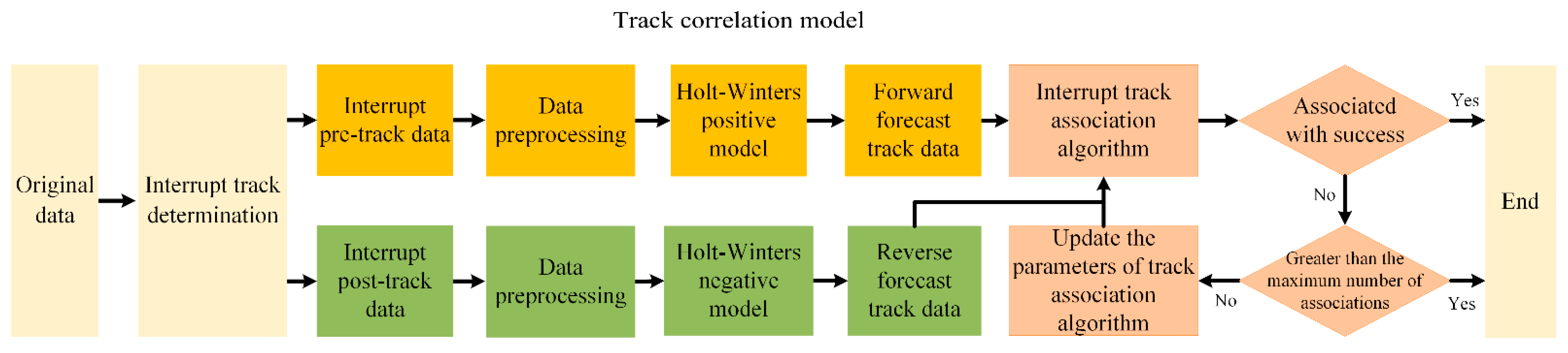
2.4. Holt-Winters Prediction and Fuzzy Analysis Model

The track model developed by this paper is shown in Figure 1. The algorithm consists of the following parts: establishing the Holt-Winters prediction model, prediction track data, and associating track segments.

• Track segment judgment: real-time judgment of incoming track points, if the latest track point is not received after the set time, it is considered that the current track is in an interrupted state, and the procedure goes to the next step;
• Track segment data processing: convert the pre-interruption track data into the format required by the program and use the processed pre-interruption track data to train the Holt-Winters forward model while waiting for the recovery of the track point. If the point data are considered to be in an interrupted state at the end of the track, the program goes to the next step;
• Track segment data prediction: the processed track data before the interruption and the track data after the interruption are processed and sent to the Holt-Winters model, and the Holt-Winters method is used to predict from two directions. After the prediction is completed, the program goes to the next step;
• Track segment association: a fuzzy track association algorithm is used to correlate data before and after interruption. If the association fails and the number of repeated associations does not exceed the preset maximum number of times, end the program. If the association fails, perform the secondary association: first jump to step 3 to update the prediction result and then replace the Equation (7) of the algorithm with Equation (9) in the fourth step of the program, and then perform the fuzzy track. The association algorithm is shown below.

3. Results

3.1. Data Set

In this paper, the Holt-Winters-AF model is verified and trained using the real aircraft track data set. There are multiple sources of orbital data. Based on the OpenSky website, this paper extracts flight data from around 8 am on 4 January 2021 (Beijing time) as the data source. The data comes from the aircraft status information sent by the aircraft at the current time. Each status information contains flight time, altitude, speed, heading, longitude, latitude, and other information. Flights whose status information length exceeds 300 (about 50 min, the average interval between two information is about 10 s) are selected for tracking. We ended up with 1259 flights.

3.2. Experimental Setup

The computer’s CPU is i7-7800x, and the GPU is TITAN XP. As TCN takes up more resources, the cloud server with TESLA V100 GPU is used for training.

The experimental scenario of this algorithm is: when an aircraft such as an airplane has a tracking interruption and then resumes the track, it is necessary to perform track association. The algorithm first predicts the track, and then uses the fuzzy association algorithm to correlate the data before and after the interruption.

3.3. Prediction Experiment

The parameters of each prediction experiment are designed as follows:

• LSTM [21,22]: The input step size is 3 and the output step size is 1; 32-layer network is used; epoch: 256; batchsize: 300.
• TCN [23]: The input step is 10, the learning rate is 1 × 10⁻³; epoch: 300.
• ARIMA [24,25,26,27,28]: The parameters of p, d, and q are 1, 0, and 0, respectively; other parameters: default.
• Prophet [29]: Parameters: default; the prediction frequency is 10 s.
• Holt-Winters: “Trend” is set to “add”. Except that, the three feature parameters x, and vx are slightly different, the “damped trend” of other feature column parameters is set to “true” and “seasonal” is set to “add”.

It is assumed that all flights resume at the same time after being interrupted at some point (In the experiment, the signal was lost when the 200th flight data was received, and the signal was restored when the 300th flight data was received. The original data are the flight data with a length of more than 300 pieces and an average interval of 10 s. The first 200 pieces of data are artificially intercepted as the input of the prediction model, and 200–300 pieces of the original data are used as the true value for comparison). Since the average transmission interval of each flight data is about 10 s, the duration of the track break is about 16.7 min (100 data points). Each piece of flight data is processed into time information, position information in three spatial directions, velocity information in three spatial directions, and acceleration information in three spatial directions. All data have been normalized.

Since all data are standardized, the errors in

Table 1. Error comparison of various prediction methods (breakage period lasts about 16.7 min).

Error	Method
	LSTM	TCN	ARIMA	Prophet	Holt-Winters
x (m)	0.01031226	0.00847442	0.00343247	0.000282	0.00036811
y (m)	0.01457218	0.01379722	0.00490498	0.000393	0.00097181
z (m)	0.0500951	0.04427563	0.02846062	0.005334	0.0077661
vx (m/s)	0.00623551	0.0041277	0.00063828	0.00068	0.000844625
vy (m/s)	0.0060439	0.00399427	0.00035111	0.000383	0.001006425
vz (m/s)	0.00608286	0.00376995	0.00048802	0.000474	0.00061313
ax (m/s2)	0.00612628	0.0041475	0.00063779	0.000683	0.00148328
ay (m/s2)	0.00591117	0.00409016	0.00034982	0.000384	0.001005105
az (m/s2)	0.00600928	0.00384299	0.00048726	0.000473	0.000612425
Time (min)	120	480	15	15	10

are standardized predicted minus standardized actual. The relative magnitudes of the error terms only represent the prediction performance of each model.

The specific calculation formula of the error is as follows:

$$Error=\left|i-\tilde{i}\right|,i\in \{x,y,z,v_x,v_y,v_z,a_x,a_y,a_z\}$$

(11)

among them, $i$ represents the 9 components ($x,y,z,v_x,v_y,v_z,a_x,a_y,a_z$) of the input feature, and $\tilde{i}$ represents the prediction result of the corresponding feature component of the model.

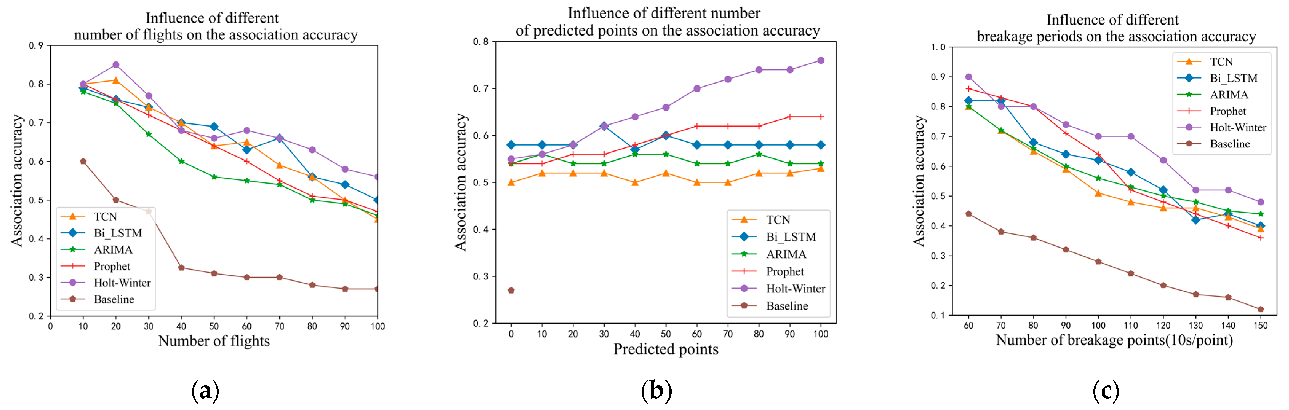
3.4. Track Association Experiment

In the track association experiment, three indicators including the number of flights, the number of forecast points, and breakage period are employed to evaluate and demonstrate the performance of the models. We use the fuzzy association method in Ref. [30] as a baseline for comparison. The following are the settings of specific parameters for each experiment. The association accuracy is the proportion of track where the association result after the original track is interrupted and is the same as the real result.

In the experiment of the effect of different flight times on the association accuracy, the first 100 data of the original data were used as the data before the interruption, the 100–200 data were used as the data at the time of interruption (about 16.7 min of interruption), and the 200th data were used after the interruption for the interrupted data. After considering the running speed of the experiment and the performance of the model, we chose to predict 50 data points (any number can be predicted). The parameters of the prediction model are the same as those in the prediction experiments described above.

In the experiment of the effect of different prediction points on the association accuracy, the first 100 data of the original data are used as the data before the interruption, the 100–200 data are used as the data at the time of interruption (interruption is about 16.7 min), and the 200th data are used as the data after the interruption for the interrupted data. In total, 50 flights are randomly selected. The parameters of the prediction model are the same as those in the prediction experiments described above.

In the experiment of the effect of different fracture periods on the association accuracy, 50 data points (any number can be predicted) are selected and predicted after comprehensively considering the running speed of the experiment and the performance of the model, and 100 flights are randomly selected from the screened 1259 flights as the subject of this experiment. The parameters of the prediction model are the same as in the previous prediction experiments.

4. Discussion

It can be seen from Table 1 that the LSTM and TCN methods based on deep learning are relatively complicated with the problems of long program running time and limited input sequence length. Furthermore, their “receptive fields” are limited and cannot perceive all the information. Therefore, methods based on deep learning are more suitable for accurately predicting changes in short-term track. As the algorithm complexity of ARIMA, Holt-Winters, and other machine learning methods is much lower than that of deep learning methods, they have global “receptive field” and can better fit the track data and bring better and faster results.

As can be seen from Figure 2a, after break-off at 100 data points (about 16.7 min), the accuracy of simultaneously associating 10 flight tracks reaches up to 90%, and the accuracy of simultaneously associating 100 flight tracks is also 60%. It is worth noting that due to the huge amount of flight data, calculating all the data on the selected 1259 tracks is a huge amount of workload. Therefore, to facilitate the comparative experiment, we randomly select a certain number of routes for the experiment. Additionally, because the algorithm has predicted 80 points, when the number of flights increases, the distance between flights becomes very close, and the predicted track may deviate from the correct track and point to other routes, resulting in decreased association accuracy.

As can be seen from Figure 2b, when break-off occurs at 100 data points (about 16.7 min) and 100 flight tracks are associated at the same time, the association accuracy increases significantly with the increase in forecast points. Therefore, prediction has played a big role.

According to Figure 2c, when 100 flight tracks are associated and 50 points on each track are predicted at the same time, the accuracy in the case of 500 s of breakage period is as high as 90%. With the increase in the breakage period, uncertainty rises and the association accuracy declines significantly. In addition, there are many hyperparameters in the programs, whose determination is directly related to the accuracy of the programs, so selecting proper hyperparameters may bring better results.

This paper presents a track segment association algorithm based on the Holt-Winters method and fuzzy track association. The algorithm first uses the Holt-Winters method to extrapolate and extend the track segment data, and then employs the fuzzy association algorithm to associate the track data. It makes full use of the track information to extrapolate and extend the track data in the case of a small amount of track segment data and uses the fuzzy track association algorithm to perform track association and secondary association. The algorithm can realize real-time track association when the target label attributes change before and after track breakage with good association ability and robustness.

Indeed, many points in this paper are yet to be improved. Firstly, as the programs mentioned in the paper involve too many hyperparameters, they will bring many problems to their application. This needs to be solved in the future. Secondly, the effect of the secondary association mechanism is not marked, and the effect of multiple associations has no obvious advantage over the effect of associating the first point after data recovery. The subsequent association correction method based on multiple points after data recovery can be further improved as well. Finally, for a fixed number of forecast points, a small number of flights for the association will bring good results, and too many forecast points from a large number of flights will often bring opposite effects. A prediction method for a better and adaptive number of track points needs further study.

5. Conclusions

This paper presents a track segment association algorithm based on the Holt-Winters bidirectional prediction and multiple fuzzy track association method. The algorithm first uses the Holt-Winters method to extrapolate and extend the track segment data in two directions, and then uses the fuzzy association algorithm to perform multiple associations on the track data. The algorithm can realize rapid track association when the target label attributes change before and after track breakage with good association ability and robustness.

The main contributions of this paper are as follows. Firstly, analyze and test the performance of existing mainstream prediction methods in track prediction. Secondly, propose a two-way track prediction algorithm based on the Holt-Winters method, and a multiple track segment association algorithm based on fuzzy track association method. Then, combine the prediction algorithm and the association algorithm to obtain the final track association algorithm.

Finally, some parts of this paper are expected to be improved. Firstly, as the programs mentioned in the paper involve too many hyperparameters, they will bring many problems to the application. This needs to be solved in the future. Secondly, for a fixed number of forecast points, a small number of flights for the association will bring good results, while too many forecast points from a large number of flights will often bring opposite effects. All in all, a prediction method for a better and adaptive number of track points needs further study.

References

1. Li, T.; Chen, H.; Sun, S.; Corchado, J.M. Joint Smoothing and Tracking Based on Continuous-Time Target Trajectory Function Fitting. IEEE Trans. Autom. Sci. Eng. 2019, 16, 1476–1483. [Google Scholar] [CrossRef] [Green Version]
2. Rong Li, X.; Jilkov, V.P. Survey of maneuvering target tracking. Part I. Dynamic models. IEEE Trans. Aerosp. Electron. Syst. 2003, 39, 1333–1364. [Google Scholar] [CrossRef]
3. Rong Li, X.; Jilkov, V.P. Survey of Maneuvering Target Tracking. Part II: Motion Models of Ballistic and Space Targets. IEEE Trans. Aerosp. Electron. Syst. 2010, 46, 96–119. [Google Scholar]
4. Rong Li, X.; Jilkov, V.P. Survey of maneuvering target tracking. Part V. Multiple-model methods. IEEE Trans. Aerosp. Electron. Syst. 2005, 41, 1255–1321. [Google Scholar] [CrossRef]
5. Zhou, J.; Li, T.; Wang, X.; Zheng, L. Target Tracking with Equality/Inequality Constraints Based on Trajectory Function of Time. IEEE Signal Process. Lett. 2021, 28, 1330–1334. [Google Scholar] [CrossRef]
6. Singer, R.A. Estimating Optimal Tracking Filter Performance for Manned Maneuvering Targets. IEEE Trans Aerosp. Electron. Syst. 1970, 6, 473–482. [Google Scholar] [CrossRef]
7. Bar-Shalom, Y.; Jaffer, A.G. Adaptive linear Filtering for Tracking with Measurements of Uncertain Origin. In Proceedings of the 1972 IEEE Conference on Decision and Control and 11th Symposium on Adaptive Processes, New Orleans, LA, USA, 13–15 December 1972. [Google Scholar]
8. Fortmann, T.E.; Bar-Shalom, Y.; Scheffe, M. Multi-target tracking using joint probabilistic data association. In Proceedings of the 19th IEEE Conference on Decision and Control including the Symposium on Adaptive Processes, Albuquerque, NM, USA, 10–12 December 1980. [Google Scholar]
9. Singer, R.A.; Sea, R.G. A New Filter for Optimal Tracking in Dense Multi-target Environments. In Proceedings of the Ninth Allerton Conference Circuit and System Theory, Monticello, VA, USA, 6–8 October 1971. [Google Scholar]
10. Reid, D.B. An Algorithm for Tracking Multiple Targets. IEEE Trans. Autom. Control. 1979, 24, 843–854. [Google Scholar] [CrossRef]
11. Blackman, S.S.; Popoli, R. Design and Analysis of Modern Tracking Systems; Artech House: Norwood, MA, USA, 1999. [Google Scholar]
12. Hachour, S.; Delmotte, F.; Mercier, D.; Lefevre, E. Object tracking and credal classification with kinematic data in a multi-target context. Inf. Fusion 2014, 20, 174–188. [Google Scholar] [CrossRef]
13. Schultz, D.; Burgard, W.; Fox, D. Tracking Multiple Moving Targets with a Mobile Robot Using Particle Filters and Statistical Data Association. IEEE Int. Conf. Robot. Autom. 2001, 2, 1665–1670. [Google Scholar]
14. Bar-Shalom, Y.; Rong Li, X.; Tugnait, J.K. Estimation with Applications to Tracking and Navigation: Theory, Algorithms and Software; Wiley-Interscience Publication: Hoboken, NJ, USA, 2001; pp. 179–490. [Google Scholar]
15. Holt, C.C. Forecasting seasonals and trends by exponentially weighted moving averages. Int. J. Forecast. 2004, 20, 5–10. [Google Scholar] [CrossRef]
16. Winters, P.R. Forecasting Sales by Exponentially Weighted Moving Averages. Math. Models Mark. A Collect. Abstr. 1976, 132, 384–386. [Google Scholar]
17. Suseelatha, A.; Sudheer, G. Short term load forecasting using wavelet transform combined with Holt-Winters and weighted nearest neighbor models. Int. J. Electr. Power Energy Syst. 2015, 64, 340–346. [Google Scholar]
18. Grubb, H.; Mason, A. Long lead-time forecasting of UK air passengers by Holt-Winters methods with damped trend. Int. J. Forecast. 2001, 17, 71–82. [Google Scholar] [CrossRef]
19. Yar, M.; Chatfield, C. Prediction intervals for the Holt-Winters forecasting procedure. Int. J. Forecast. 1990, 6, 127–137. [Google Scholar] [CrossRef]
20. Gelper, S.; Fried, R.; Croux, C. Robust forecasting with exponential and Holt–Winters smoothing. J. Forecast. 2010, 29, 285–300. [Google Scholar]
21. Hochreiter, S.; Schmidhuber, J. Long Short-Term Memory. Neural Comput. 1997, 9, 1735–1780. [Google Scholar] [CrossRef]
22. Graves, A.; Schmidhuber, J. Framewise phoneme classification with bidirectional LSTM and other neural network architectures. Neural Netw. 2005, 18, 602–610. [Google Scholar] [CrossRef]
23. Bai, S.; Zico Kolter, J.; Koltun, V. An Empirical Evaluation of Generic Convolutional and Recurrent Networks for Sequence Modeling. arXiv 2018, arXiv:1803.01271v2. [Google Scholar]
24. Xu, F.; Du, Y.A.; Chen, H.; Zhu, J.M. Prediction of Fish Migration Caused by Ocean Warming Based on SARIMA Model. Complexity 2021, 2021, 5553935. [Google Scholar] [CrossRef]
25. Kirbas, I.; Sozen, A.; Tuncer, A.D.; Kazancioglu, F.S. Comparative analysis and forecasting of COVID-19 cases in various European countries with ARIMA, NARNN and LSTM approaches. Chaos Solitons Fractals 2020, 138, 110015. [Google Scholar] [CrossRef]
26. Aasim; Singh, S.N.; Mohapatra, A. Repeated wavelet transform based ARIMA model for very short-term wind speed forecasting. Renew. Energy 2019, 136, 758–768. [Google Scholar] [CrossRef]
27. Ordonez, C.; Sanchez Lasheras, F.; Roca-Pardinas, J.; de Cos Juez, F.J. A hybrid ARIMA-SVM model for the study of the remaining useful life of aircraft engines. J. Comput. Appl. Math. 2019, 346, 184–191. [Google Scholar] [CrossRef]
28. De Oliveira, E.M.; Cyrino Oliveira, F.L. Forecasting mid-long term electric energy consumption through bagging ARIMA and exponential smoothing methods. Energy 2018, 144, 776–788. [Google Scholar] [CrossRef]
29. Taylor, S.J.; Letham, B. Forecasting at Scale. Am. Stat. 2018, 72, 37–45. [Google Scholar] [CrossRef]
30. Jian, D.; Xuezhi, X. A Fuzzy Track Association Algorithm in Track Interrupt-oriented. Fire Control. Command. Control. 2013, 38, 518–522. [Google Scholar]
Figure 1. Flow chart of the track association algorithm.
Aerospace 09 00274 g001
Figure 2. The results of track association experiment: (a) Influence of a different number of predicted points on the association accuracy; (b) Influence of a different number of predicted points on the association accuracy (The baseline is the method that does not make predictions); (c) Influence of different breakage periods on the association accuracy.
Aerospace 09 00274 g002