Coordinated Formation Guidance Law for Fixed-Wing UAVs Based on Missile Parallel Approach Method

Abstract

This paper presents a classic missile-type parallel-approach guidance law for fixed-wing UAVs in coordinated formation flight. The key idea of the proposed guidance law is to drive each follower to follow the virtual target point. Considering the turning ability of each follower, the formation form adopts the semi-perfect rigid form, which does not require the vehicle positions form a rigid formation, and the orientations keep consensus. According to the mission characteristics of the follower following a leader and the leader following a route, three guidance laws for straight, turning, and circling flight are designed. A series of experiments demonstrate the proposed guidance law’s improved response and maneuvering stability. The results of hardware-in-the-loop simulations and real flight tests prove that the proposed guidance law satisfies the practical UAV formation flight control demands.

1. Introduction

After decades of development, UAV technology has evolved from single-handed function expansion into collaborative mission design. Single UAVs have limitations, such as the specific functions they can execute and a limited range of onboard sensors. These issues necessitate the collaboration of multiple UAVs [1,2]. In the military, UAV formations aim to make tactical decisions on their own and create teams to collaborate towards high-level goals [3,4,5], allowing a single person to command a fleet of UAVs. Therefore, it is necessary to design a planning algorithm for the autonomous coordination of UAVs in formation flight [6,7].

There has been considerable theoretical and practical research on UAV formation control. Joongbo S. [8] propose a consensus-based feedback linearization method to maintain a specified time-varying geometric configuration for formation flight of multiple autonomous vehicles. In this approach, any explicit leader does not exist in the formation team, and therefore the proposed control strategy requires only the local neighbor-to-neighbor information between vehicles. In reference [9], the synchronized position tracking controller is incorporated in formation flight control for multiple flying wings, the performance and effectiveness of the formation controller are improved when the virtual structure approach is utilized to maintain formation geometry; Zhang, J.M. [10] describes a path-following method based on a virtual target for fixed-wing UAVs, allowing sudden flight path changes to be anticipated and acute heading changes to be avoided. Zhang, M. [11] presents a method of guidance law for cooperative tracking based on leader-follower formation of UAVs, which solves the problem of speed range limitation of traditional standoff tracking method. In Reference [12], model-based modified nonlinear guidance law is proposed so that a lateral acceleration command generated by the proposed guidance law coincides with actual lateral acceleration of the UAV. Utilizing the proposed nonlinear guidance law, leader-follower formation flight controller is designed.

Unlike most of the existing literature investigating multi-UAV formation flying problems, which mainly focus on controller design in order to achieve desired configurations, there are few studies on the control law design of semi-rigid formations. This work aims at designing a low-speed fixed-wing UAV cooperative formation guidance law to form a semi-perfect rigid formation. Compared with perfect rigid formations and flexible formations, semi-perfect rigid formations have certain advantages. Semi-perfect rigid formations are more flexible than perfect rigid formations. When the UAV formation turns, for perfect rigid formations, it is required that not only the vehicle positions form a rigid formation, but also the orientations keep consensus. However, for semi-perfect rigid formations, the orientation requirement is ignored. In addition, flexible formation is not necessarily more agile than semi-perfect rigid formation with the same formation width, due to the special stall speed constraint of fixed-wing UAVs [13].

The leader–follower method is employed as the primary mode of cooperative formation control in the present study. During formation flying, the leader aircraft flies along the mission path, and the guidance law of leader keeps the lateral heading and longitudinal position stable while ensuring the leader aircraft stays as close to the route as possible. The guidance law of followers based on parallel approach method when the follower is flying with the leader is to guide the follower to dynamically track the points generated by the leader’s position and the spatial formation parameters. When the leader performs complex movements, the followers only need to follow the leader to fly according to the guidance law. To a certain extent, the flexibility of UAV formation changes has been greatly improved.

The remainder of this paper is organized as follows. Section 2 analyzes the motion relationship between UAVs in a collaborative formation. Section 3 gives the control laws of the leader and follower, and analyzes the simulation results. The procedures and data analysis for hardware-in-the-loop simulations and real flight test are given in Section 4, while final conclusions and future work recommendations are stated in Section 5.

2. Motion Analysis

This section gives the planar kinematics of the leader and the followers. And the motion capability of multi-UAV formation is considered to facilitate the design of motion planning algorithm at the kinematic level. The key idea of the guidance algorithm based on the missile-type parallel approach method is to drive each follower to follow the virtual target. Considering the turning ability of followers, the formation form adopts the semi-perfect rigid form, which does not require the follower to follow the virtual point with fixed heading.

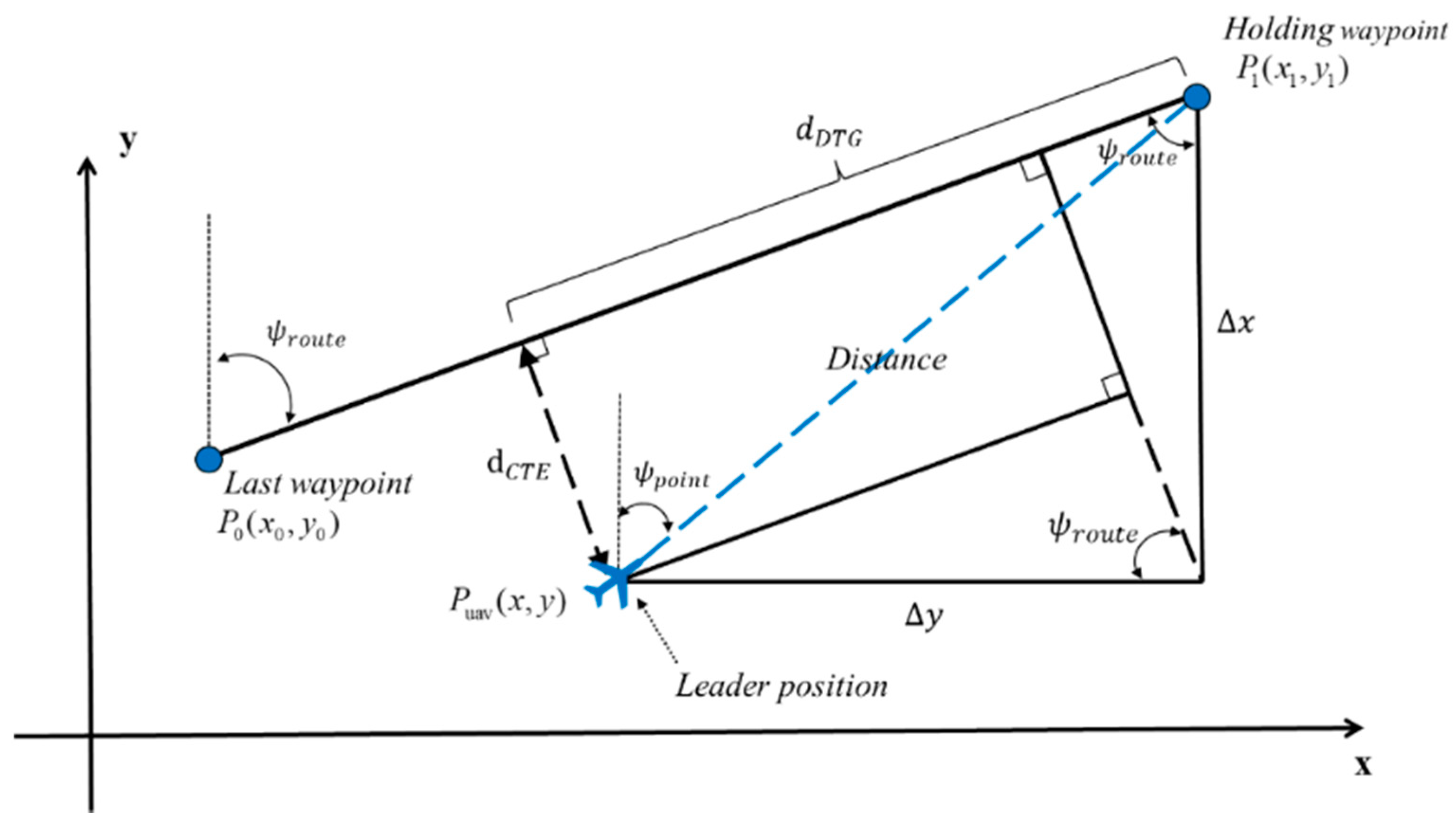
2.1. Planar Kinematics of a UAV

In this paper, it is assumed that each UAV flies at a constant altitude and only the lateral components of the UAV motion in a 2D region are considered. Thus, the planar kinematics of a UAV considered in this paper can be given as follows.

$$\left\{\begin{array}{l}{\dot{x}}_{*}=v_{*}\cos {\psi }_{*}\\ {\dot{y}}_{*}=v_{*}\sin {\psi }_{*}\\ {\dot{\psi }}_{*}={\omega }_{*}\end{array}\right.$$

(1)

where $*\in \left\{L,F\right\}$, $L$ represents the formation leader and $F$ is the follower. $x,y$ and $\psi$ are the position and heading angle of the vehicle respectively, $v$ and $\omega$ are the speed and heading rate of the vehicle respectively.

Furthermore, the speed and heading rate of a fixed-wing UAV are subject to the following motion constraints.

$$v_{\min }\le v_{*}\le v_{\max },\left|{\omega }_{*}\right|\le {\omega }_{\max }$$

(2)

where $v_{\min }$, $v_{\max }$ and ${\omega }_{\max }$ are all positive constants.

2.2. Virtual Target Point of Later Plane

The ground coordinate system is used to establish the relative positional relationship diagram in the horizontal direction of the two-dimensional scene shown in Figure 1. The leader’s position is ${[x_L\hspace{1em}{y}_L]}^T$, the follower’s position is ${[x_F\hspace{1em}{y}_F]}^T$, the speed vectors of UAV are $V_F$, $V_L$, and the direction angle of UAV are ${\psi }_L$, ${\psi }_F$, the heading angular velocity of UAV is ${\omega }_L$ and ${\omega }_F$. The above variables are brought into Equation (1) to get the velocity component and the heading angular acceleration of leader and follower.

The leader aircraft’s lateral heading motion is a circle with radius $R_L$. The flight trajectory changes $R_L$ dynamically; linear motion occurs in the special case where $R_L$ tends to $+\infty$. By shifting the leader’s position by ${\mathit{\rho }}_d$, a virtual dynamic tracking point is created. The length of ${\mathit{\rho }}_d$ is $\left|{\mathit{\rho }}_d\right|=\sqrt{\Delta x^2+\Delta y^2}$, where $\Delta x$ is the formation’s set horizontal and lateral offset distance and $\Delta y$ is the formation’s set vertical and longitudinal offset distance. The result is a virtual dynamic tracking point with a radius $R_L{}^{\prime }$, position ${[x_L{}^{\prime }\hspace{1em}{y}_L{}^{\prime }]}^T$, and velocity vector ${\mathit{V}}_L^{\prime }$. The relationship between ${\mathit{V}}_L^{\prime }$ and ${\mathit{V}}_F^{\prime }$ is as follows:

$${\mathit{V}}_L^{\prime }={\mathit{V}}_F+{\omega }_L\times {\mathit{\rho }}_d$$

(3)

where ${\omega }_L$ is the heading angular velocity of the leader.

The leader’s lateral heading control goal is to eliminate the lateral deviation caused by the flight mission. The follower’s lateral heading motion control goal is to eradicate the heading angle deviation between its position and the virtual dynamic tracking point. The following guidance law corrects this deviation.

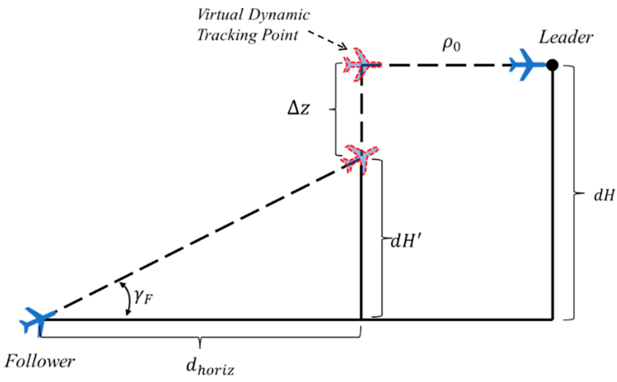
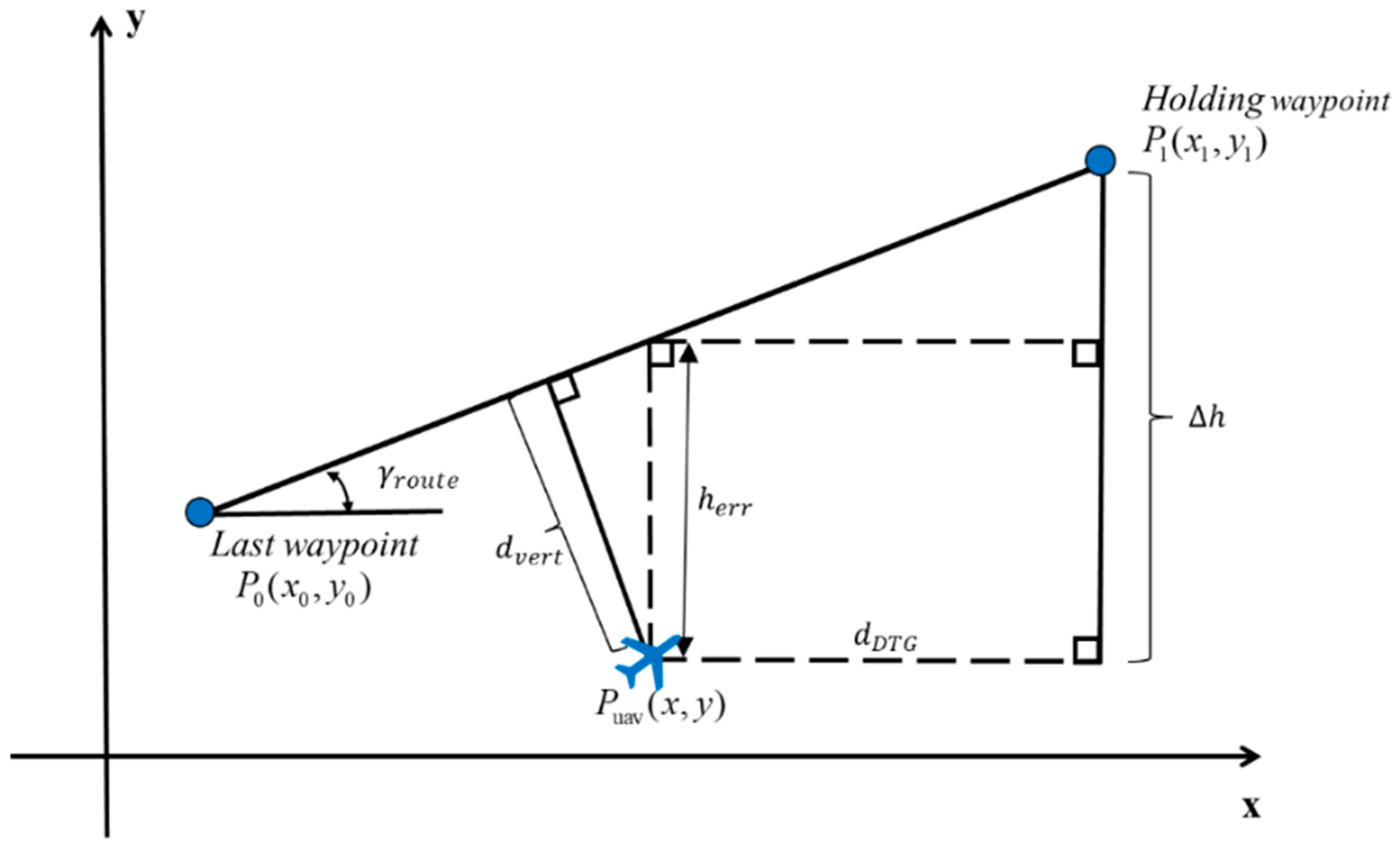
2.3. Longitudinal Motion Analysis

The position of the virtual dynamic tracking point in the vertical direction is shown in Figure 2. As the formation requires formation control in the standing order, the formation’s shear deviation value will be set according to the formation requirement in the vertical direction. The height difference between the follower and the leader is $d_H$. The height difference between the follower and the virtual dynamic tracking point in the vertical direction $d_H{}^{\prime }$ can then be calculated as:

$$d_H^{\prime }=d_H-\Delta z$$

(4)

The control goal of the vertical movement of the UAV formation is to eliminate the height difference $d_H{}^{\prime }$. The target climb angle ${\gamma }_F$ of the follower can be obtained as:

$${\gamma }_F={\tan }^{-1}(\frac{d_H^{\prime }}{d_{horiz}})$$

(5)

According to the value of the climb angle, the control command ${\theta }_c$ of the pitch channel of the follower can be calculated. This allows attitude control to be realized through the control law of the longitudinal height channel designed above.

The speed of the follower should be controlled to minimize the distance difference $\rho$ between the follower and the dynamic tracking point:

$$\rho =\sqrt{d_{horiz}^2+d_H^{\prime }{}^2}$$

(6)

The proposed method uses PI control since the fixed-wing UAV’s speed control channel has a lengthy delay and low bandwidth. The input of the control law is the distance difference $\rho$, while the output is the speed command $V_c$.

3. Guidance Law Design

The cooperative formation in this chapter adopts the “leader-follower” mode [14,15]. The navigation deviation equation of the route composed of straight line and arc under formation motion is given, and the corresponding guidance law is proposed [16]. The follower guidance law based on missile parallel approach method is given, which can give the direction angle instruction to guide the follower to the virtual point. Finally, the simulation results indicate the guidance law can create a good formation and satisfies the reaction time and steady tracking requirements.

3.1. Leader Guidance Law

The direction of the current route and the direction of the following route can determine the position and relative flying direction of the leader aircraft close to the route. In the ground coordinate system [17,18], it is assumed that the present waypoint’s coordinates are $P(x_1,y_1)$, the previous waypoint’s coordinates on the horizontal aircraft are $P(x_0,y_0)$, and the next waypoint’s coordinates are $P(x_2,y_2)$. The direction ${\psi }_{route}$, inclination angle ${\gamma }_{route}$, and distance $d_{route}$ of the current route are then calculated as follows:

$$\left\{\begin{array}{l}{d}_{route}=\sqrt{{(y_1-y_0)}^2+{(x_1-x_0)}^2}\\ {\psi }_{route}={\tan }^{-1}(\frac{y_1-y_0}{x_1-x_0})\\ {\gamma }_{route}={\tan }^{-1}(\frac{h_{d1}}{d_{route}})\end{array}\right.$$

(7)

where $h_{d1}$ is the height difference between the current waypoint and the previous waypoint. We calculate the direction ${{\psi }^{\prime }}_{path}$, inclination angle ${{\gamma }^{\prime }}_{path}$, and distance ${d^{\prime }}_{route}$ for the next route similarly.

When the UAV flies over a waypoint at which it needs to turn, the angle around the inscribed circle to give the correct change in heading can be calculated from the azimuth of the current route and that of the next route. The formula is as follows:

$$\Delta \psi ={\psi }_{path}^{\prime }-{\psi }_{path}$$

(8)

Let $\Delta \psi$ be in the interval $\left(-\mathsf{\pi },\mathsf{\pi }\right)$ and define the advance turning distance $d_{pre}$ as the distance from the tangent point between the inscribed arc trajectory and the route to the next waypoint. Neglecting the deviation from the UAV to the flight path, the approximation of $d_{pre}$ is:

$$d_{pre}=R\times \tan (\frac{\Delta \psi }{2})$$

(9)

where $R$ is the turning radius parameter of the next waypoint.

• Linear navigation mode

In the ground coordinate system, the real-time position coordinates of the leader are $P_{UAV}(x,y)$, the coordinates of the previous waypoint are $P(x_0,y_0)$, and the coordinates of the next waypoint are $P(x_1,y_1)$, The vertical distance between the aircraft and the route is the side offset distance $d_{CTE}$, which reflects the lateral distance between the aircraft and the route. The offset is defined as positive when the plane is on the right side of the route. The projection of the distance between the aircraft position and the next waypoint on the route is the distance to be passed, denoted as $d_{DTG}$, which is positive when the aircraft passes the target point and negative otherwise. The distance to fly is an important parameter for judging whether or not to cut to the next waypoint.

As shown in Figure 3, the azimuth of the route is ${\psi }_{route}$ and the azimuth between the leader aircraft and the next waypoint is ${\psi }_{point}$. From the geometric relationship in the figure, it can be seen that $\Delta x$ and $\Delta y$ are the projections of the distance of the leader aircraft relative to the next waypoint $P_1(x_1,y_1)$ in the coordinate system. The side offset distance $d_{CTE}$ between the leader aircraft and the route is as follows:

$$d_{CTE}=\Delta x\sin {\psi }_{route}-\Delta y\cos {\psi }_{route}$$

(10)

In the same way, the distance $d_{DTG}$ between the leader aircraft and the next waypoint can be obtained as:

$$d_{DTG}=\Delta x\cos {\psi }_{route}+\Delta y\sin {\psi }_{route}$$

(11)

The purpose of the guidance law in the vertical longitudinal direction, such as the guidance law in the aircraft, is to identify the distance deviation between the UAV and the route in the vertical direction. As shown in Figure 4, the height difference between the leader aircraft and the next waypoint is $\Delta h$. From the geometric relationship, the height difference $h_{err}$ between the leader aircraft and the route in the vertical direction of the ground coordinate system can be calculated as:

$$h_{err}=\Delta h-d_{DTG}\tan {\gamma }_{route}$$

(12)

The longitudinal deviation $d_{vert}$ between the leader aircraft and the route can also be calculated. The formula is as follows:

$$d_{vert}=h_{err}\cos {\gamma }_{route}$$

(13)

The longitudinal deviation $d_{vert}$ between the leader aircraft and the route and the route inclination angle ${\gamma }_{route}$ are then used as guidance commands to control the UAV to approach the target route in the vertical direction.

2.

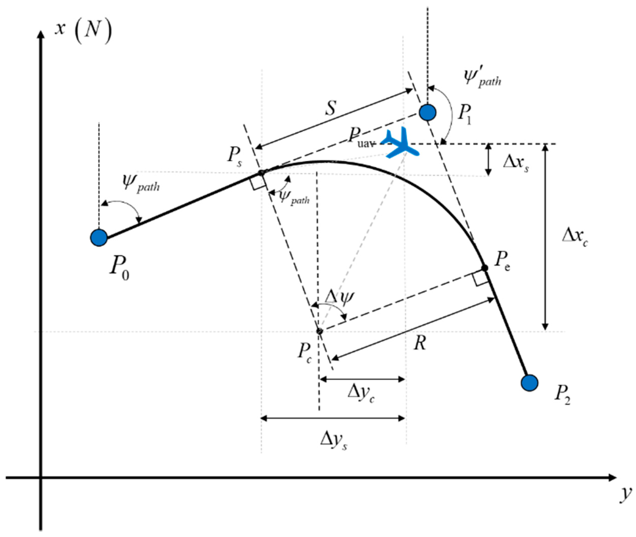
Turn navigation mode

The turn guidance comprises a quarter arc and two straight lines. The relative location of the leader aircraft and the waypoint are used to calculate parameters such as the route direction, longitudinal deviation, route curvature angular velocity, and side offset distance. These parameters are input into the controller to compute the turn control of the lead aircraft. The turning radius is a known parameter, while the center of the arc and the position of the tangent point to the straight line must be determined. The relationship between the UAV’s flight trajectory and waypoints in turn guidance mode is shown in Figure 5.

As shown in Figure 6, $P_s$ is the initial turning point, $P_s$ is the final turning point, and the radius of the turning route is $R$. The turning center angle $\Delta \psi$ is calculated as follows:

$$\Delta \psi ={\psi }_{route}^{\prime }-{\psi }_{route}$$

(14)

where ${\psi }_{route}$ is the angle between the line segment $P_0{P}_1$ and true north and ${{\psi }^{\prime }}_{point}$ is the angle between the line segment $P_1{P}_2$ and true north, calculated from Equation (7). The range of $\Delta \psi$ is (−π, π). If the value exceeds this range, it needs to be processed into the interval (−π, π) by adding or subtracting 2π. When $\Delta \psi >0$, the UAV makes a clockwise turn; otherwise, it creates a counterclockwise turn.

The turning distance $d_{pre}$ is calculated by Equation (9). Combined with the relative positions $\Delta x$, $\Delta y$ and $\Delta h$ of the UAV and the track point $P_1$, the relative positional relationship between the UAV and the initial turning point $P_s$ and final turning point $P_e$ can be calculated. The formulas are as follows:

$$\left\{\begin{array}{c}\Delta x_s=\Delta x-d_{pre}\cos {\psi }_{route}\\ \Delta y_s=\Delta y-d_{pre}\cos {\psi }_{route}\\ \Delta h_s=\Delta h-d_{pre}\cos {\psi }_{route}\end{array}\right.$$

(15)

$$\left\{\begin{array}{c}\Delta x_e=\Delta x-d_{pre}\cos {\psi }^{\prime }{}_{route}\\ \Delta y_e=\Delta y-d_{pre}\cos {\psi }^{\prime }{}_{route}\\ \Delta h_e=\Delta h-d_{pre}\cos {\psi }^{\prime }{}_{route}\end{array}\right.$$

(16)

The relative positional relationship between the UAV and the initial turning point $P_s$ and final turning point $P_e$ can be combined with the turning distance $d_{pre}$, relative positions $\Delta x$, $\Delta y$ and $\Delta h$ of the UAV, and the track point $P$.

During the turn, the angle ${\gamma }_{route}$ is calculated as:

$${\gamma }_{route}=\arctan (\frac{\Delta h_e-\Delta h_s}{R\ast \left|\Delta \psi \right|})$$

(17)

Before and after the leader aircraft makes a turn, the guidance law is the same as straight flight. The difference is that the two tangent points $P_s$ and $P_e$ are virtual track points for straight-line guidance. Whether to perform turn guidance is determined by the distance to the waypoint $P_1$ and the distance $d_{seg}$ to the next turn.

The relative position of the UAV and the tangent point $P_s$ are given by Equation (15). The relative position relationship between the UAV and the circle center $P_c$ can then be calculated as:

$$\left\{\begin{array}{c}\Delta x_c=\Delta x_s-R\cos {\psi }_{route}\\ \Delta y_c=\Delta y_s-R\cos {\psi }_{route}\end{array}\right.$$

(18)

From the above formula, the azimuth angle $\psi$ of the arc route of the lead aircraft during the turning process can be calculated as:

$$\psi =\arctan (\frac{\Delta x_c}{\Delta y_c})-\mathsf{\pi }$$

(19)

The range of $\Delta \psi$ is (−π, π). If the value exceeds this range, it needs to be processed into (−π, π) by adding or subtracting 2π. The turning side offset distance $d_{CTE}$ of the lead aircraft and the curvature $\omega$ of the route are used as input commands for the lateral heading guidance. The calculation formula is as follows:

$$\left\{\begin{array}{c}{d}_{CTE}=R-\sqrt{\Delta x_c^2-\Delta y_c^2}\\ \omega =\frac{V_L}{R}\end{array}\right.$$

(20)

In turn guidance mode, the longitudinal control is similar to the longitudinal direction in straight guidance mode.

3.

Hovering mode

The minimum airspeed limits the flight of fixed-wing UAVs, and since some specific reconnaissance scenarios require the UAVs to stay in a fixed area for a long time, hovering mode can be used to handle the repeated circling of a set waypoint. Taking the sample UAV in this paper as an example, the actual flight trajectory of hovering mode is shown in Figure 7.

To make a circling motion after entering hovering mode, the leader aircraft uses the current waypoint as the center of the circle and the radius parameter R of the waypoint as the radius. Hovering navigation parameters are calculated in the same way as turning navigation parameters. Figure 8 shows a schematic diagram of the guidance law. When the UAV hovers clockwise, the current route azimuth is ${\psi }_{L1}$; when it hovers counterclockwise, the current route azimuth is ${\psi }_{L2}$. Therefore, when circling clockwise, the azimuth angle ${\psi }_{iangle}$ is calculated as follows:

$${\psi }_{iangle}={{\psi }^{\prime }}_{route}-{\psi }_{L1}$$

(21)

The value range of ${\psi }_{iangle}$ is (−π, π). If the value exceeds this range, it needs to be processed into (−π, π) by adding or subtracting 2π. When ${\psi }_{iangle}>0$, the UAV will perform a clockwise turn; otherwise, it makes a counterclockwise turn.

We calculate $d_{DTG}$ as follows:

$$d_{DTG}=\left|{\psi }_{iangle}\right|·R$$

(22)

In hovering mode, longitudinal guidance is similar to linear flight mode.

3.2. Follower Guidance Law

• Calculation of lateral virtual dynamic tracking points

The analysis in the previous section indicates that the virtual dynamic tracking point for lateral movement must be calculated using the formation distance parameters $\Delta x$ and $\Delta y$. The tracking target of the follower is the virtual active tracking point. It is assumed that the UAVs are all particles when they fly in formation. As in Figure 9, the leader’s location is point A, the position of the virtual dynamic tracking point is point B, and the location of the follower is point C.

The formation coordinate system $O_f{X}_f{Y}_f{Z}_f$ is fixed around the leader aircraft L, with the origin $O_f$ placed at the leader’s center of mass [19]. The $O_f{X}_f$ axis points forward along the speed vector direction of the leader aircraft; the $O_f{Y}_f$ axis is perpendicular to the $O_f{X}_f$ axis and points to the right of the flight direction; the $O_f{Z}_f$ axis is perpendicular to the $O_f{X}_f{Y}_f$ axis and points downward. In the two-dimensional scene, the coordinates of the horizontal virtual dynamic tracking point B are calculated on the plane $O_f{X}_f{Y}_f$. The region between points A and B is shown in Figure 9. Points B and A lie on concentric circles with arc lengths of $arc$ and $\Delta x$, respectively, $\Delta y$ is the straight-line length between the circles, and $R_L$ is the flight radius of the lead aircraft. In this coordinate system, the coordinate difference between points B and A is $\Delta x_e$ and $\Delta y_e$. Through the geometric relationship, the lengths of $\Delta x_e$ and $\Delta y_e$ can be obtained.

When the included angle $\phi$ is small:

$$\left\{\begin{array}{l}\Delta x_e=arc\\ \Delta y_e=\Delta y\end{array}\right.$$

(23)

and when the included angle φ is larger:

$$\left\{\begin{array}{l}\Delta x_e=\frac{arc}{\phi }\phi \\ \Delta y_e=\Delta y-\frac{arc}{\phi }\phi (1-\cos \phi )\end{array}\right.$$

(24)

where $arc$ is calculated as follows:

$$arc=(1+\frac{1}{R}\Delta y)\Delta x$$

(25)

Therefore, the distance difference ${[\Delta x_e\hspace{1em}\Delta y_e]}^T$ between the virtual dynamic tracking point B and the leader A can be obtained through the distance ${[\Delta x\hspace{1em}\Delta y]}^T$ set by the formation.

The transformation matrix of the formation coordinate system $O_f{X}_f{Y}_f{Z}_f$ from the ground coordinate system $O_g{X}_g{Y}_g{Z}_g$ is:

$$L_{gf}=\left[\begin{array}{cc}\cos {\psi }_L& \sin {\psi }_L\\ -\sin {\psi }_L& \cos {\psi }_L\end{array}\right]$$

(26)

where ${\psi }_L$ is the angle between the two vector axes $O{x}_f$ and $O{x}_g$.

Then, the coordinate difference between points A and B in the ground coordinate system is:

$$\left[\begin{array}{c}\Delta x_e^{\prime }\\ \Delta y_e^{\prime }\end{array}\right]=L_{gf}\left[\begin{array}{c}\Delta x_e\\ \Delta y_e\end{array}\right]$$

(27)

It can be seen that the coordinates of point B are:

$$\left[\begin{array}{c}{x}_L^{\prime }\\ y_L^{\prime }\end{array}\right]=\left[\begin{array}{c}{x}_L-\Delta x_e^{\prime }\\ y_L-\Delta y_e^{\prime }\end{array}\right]$$

(28)

Let the distance difference between points B and C be T. Then, we have:

$$\left[\begin{array}{c}{p}_x\\ p_y\end{array}\right]=\left[\begin{array}{c}{x}_F-x_L^{\prime }\\ y_F-y_L^{\prime }\end{array}\right]$$

(29)

2.

Collaborative guidance law design

Geometric methods are commonly used in engineering practice. Existing geometric guidance laws include pure line-of-sight tracking, proportional guidance, and the parallel approach. These three guidance methods and selection principles are compared in

Table 1. Comparison of different guidance methods.

Guidance Law	Overload	Trajectory	Mobility
Line-of-sight tracking	Large	Curved	Poor
Proportional guidance	Small	Slightly curved	Strong
Parallel approach	Small	Straight	Strong

.

It can be seen from Table 1 that the parameter index of the parallel approach method is better suited to the task of formation flying, but its technical implementation is more complicated. The main difficulty lies in the real-time observation of the speed $V_m$ and the azimuth angle ${\eta }_m$ of the target. In the leader-follower control mode considered in this paper, the leader aircraft sends real-time status information through an airborne data link, and the follower can obtain $V_m$ and ${\eta }_m$ of the leader aircraft through a relatively simple calculation. Therefore, the parallel approach method guides the follower to the virtual dynamic tracking point.

The realization of the parallel approach method involves keeping the line-of-sight angle $q$ between the follower and the dynamic tracking point unchanged during the flight. In the ground coordinate system, the line-of-sight angle between the follower and the active tracking point is $q$, and the angle between the velocity vector and the line-of-sight direction is defined as the lead angle, as shown in Figure 10. The flight speed of the follower is $V_F$, the speed azimuth is ${\psi }_F$, and the lead angle is ${\eta }_F$. The flight speed of the dynamic tracking point is $V_L{}^{\prime }$, the speed azimuth is ${\psi }_F{}^{\prime }$, and the lead angle is ${\eta }_F{}^{\prime }$. The horizontal straight-line distance between the follower and the dynamic tracking point is $d_{horiz}$.

The following geometric relationships exist between the lead angle, velocity azimuth angle, and line-of-sight angle of the follower and the dynamic tracking point:

$$\left\{\begin{array}{c}{\eta }_F=q-{\psi }_F\\ {\eta }_L^{\prime }=q-{\psi }_L^{\prime }\end{array}\right.$$

(30)

The relative motion speed ${\dot{d}}_{horiz}$ between the follower and the dynamic tracking point is:

$${\dot{d}}_{horiz}=V_F\cos {\eta }_F-V_L^{\prime }\cos {\eta }_L^{\prime }$$

(31)

and the change in the line-of-sight angle between the follower and the dynamic tracking point is:

$$\dot{q}=\frac{1}{d_{horiz}}(V_L^{\prime }\sin {\eta }_L^{\prime }-V_F\sin {\eta }_F)$$

(32)

The above two formulas are the guiding equations of the parallel approach method. The constraints are:

$$\epsilon =\dot{q}=0$$

(33)

where $q$ can be calculated from the position of the follower and the position of the dynamic tracking point. As shown in Figure 9, the coordinate difference between points B and C is ${[P_x\hspace{1em}{P}_y]}^T$, and the positional relationship is as shown in Figure 10. Thus, $q$ is calculated as:

$$q={\tan }^{-1}(\frac{p_y}{p_x})$$

(34)

Now, $V_L^{\prime }\sin {\eta }_L^{\prime }$ is the projection of the velocity of the dynamic tracking point in the normal direction to the line-of-sight, $v_{normal}$ in Figure 10. The position difference vector between the follower and the virtual dynamic point is $\mathit{P}={[P_x\hspace{1em}{P}_y]}^T$, and the speed vector of the active virtual point is $\mathit{v}={[{v^{\prime }}_n\hspace{1em}{v^{\prime }}_e]}^T$. Then, $\mathit{P}·\mathit{v}=\left|\mathit{P}\right|\left|\mathit{v}\right|\cos {{\eta }^{\prime }}_L$, where $\left|\mathit{v}\right|\cos {\eta }_L^{\prime }$ is the speed of the dynamic virtual point $V_L{}^{\prime }$ along with the vector P, which is the tangential projection of $v_{horiz}$.

$$v_{horiz}=\left|\mathbf{v}\right|\cos {\eta }_L^{\prime }=\frac{(p_x{v}_n^{\prime }+p_y{v}_e^{\prime })}{\left|\mathrm{P}\right|}$$

(35)

which can also be expressed as:

$$v_{horiz}={\left[\begin{array}{cc}\frac{p_x{v}_{horiz}}{\left|\mathrm{P}\right|}& \frac{p_y{v}_{horiz}}{\left|\mathrm{P}\right|}\end{array}\right]}^T$$

(36)

The normal projection of the velocity $V_L{}^{\prime }$ of the dynamic virtual point on the vector $\overrightarrow{P}$ is denoted as ${\mathit{v}}_{normal}=\mathit{v}-{\mathit{v}}_{horiz}$. The modulus of ${\mathit{v}}_{normal}$ is $\left|{\mathit{v}}_{normal}\right|$, and the expected heading control command of the follower can be obtained as:

$${\psi }_{Fc}=q-{\sin }^{-1}(\frac{\left|v_{normal}\right|}{V_F})$$

(37)

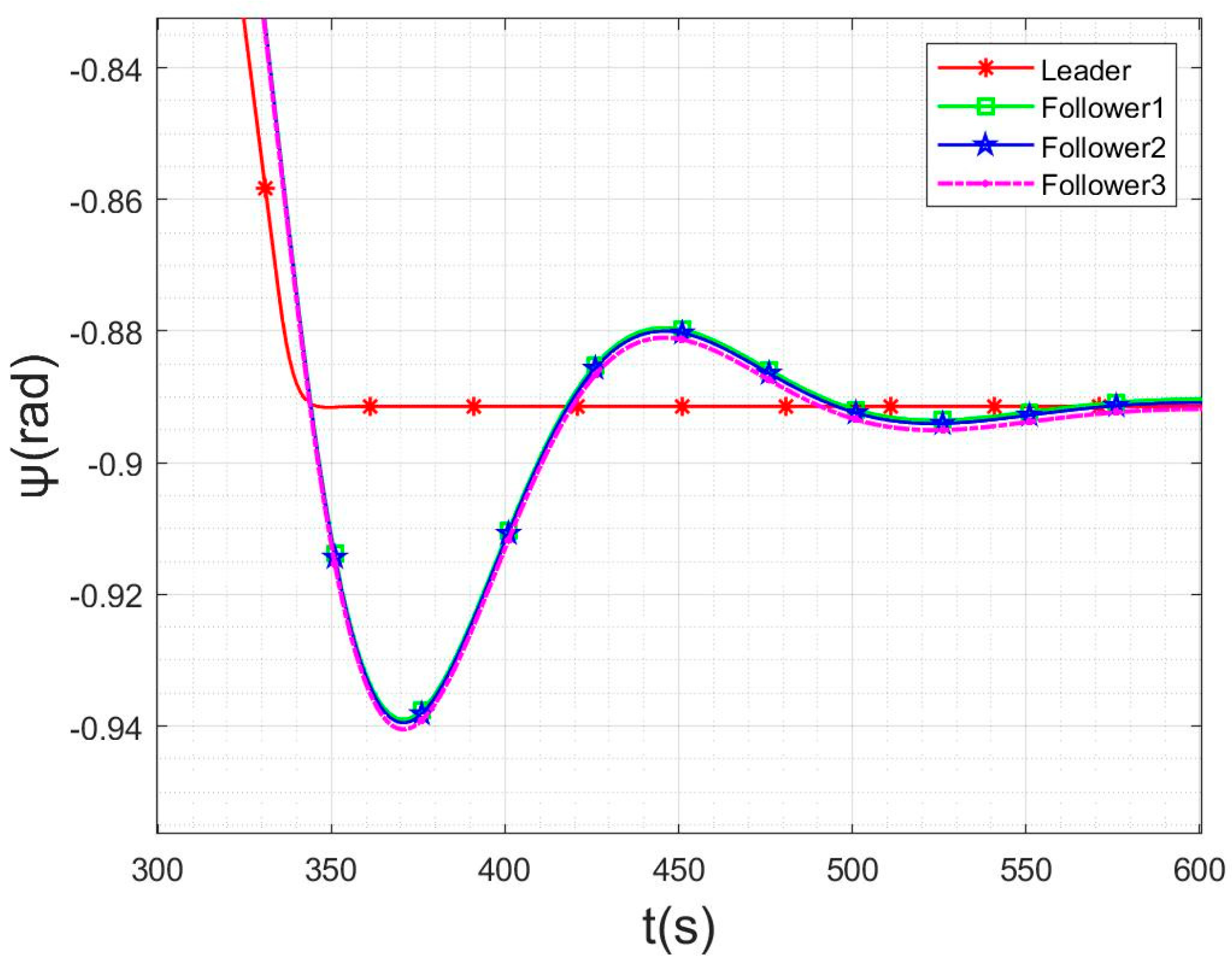
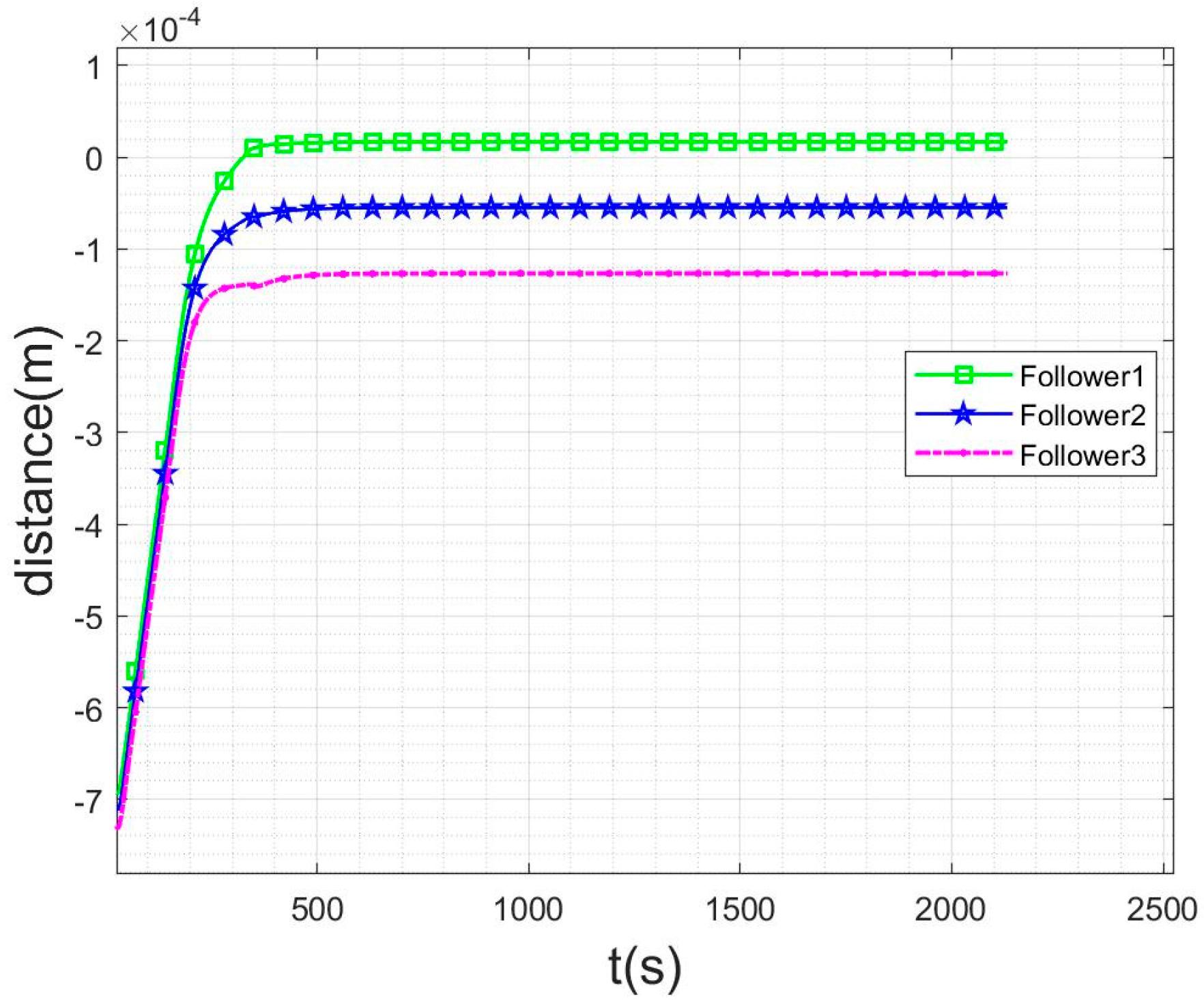
3.3. Guidance Law Simulation Verification Results

The core index of the guidance law using the parallel approach method is the tracking effect of the heading channel. Figure 11 shows the dynamic change in the heading angle of the leader and three followers with time. When the heading of the leader aircraft changes rapidly, the heading channels of the three followers can respond and track in time. When the leader aircraft’s heading becomes stable, the followers can smoothly track the leader after a small amount of overshoot. This shows that the follower’s guidance law can make the follower ‘s heading angle converge to the target heading angle quickly.

We now modify the formation distance parameter in the input to the simulation model and set it to a triangular formation. Figure 12 shows a visual representation of the flight route based on the simulation findings. The shape of the collaborative formation is well maintained, as may be seen intuitively. The relative position difference between each follower and the leader is depicted in Figure 13. After the formation flight begins, the followers swiftly spread out and maintain a consistent distance from the leader during tracking.

In conclusion, the guidance law proposed in this paper creates a good formation and satisfies the reaction time and steady tracking requirements. It is also suitable for semi-physical simulations and actual flight.

4. Flight Verification

4.1. Hardware-in-the-Loop Simulations

The high-precision algorithm has stringent hardware requirements. otherwise, it would significantly impact dynamic position tracking control accuracy and real-time performance. Hardware-in-the-loop simulations [20,21] are performed for the specified formation guidance laws to ensure compatibility between the algorithm and the hardware.

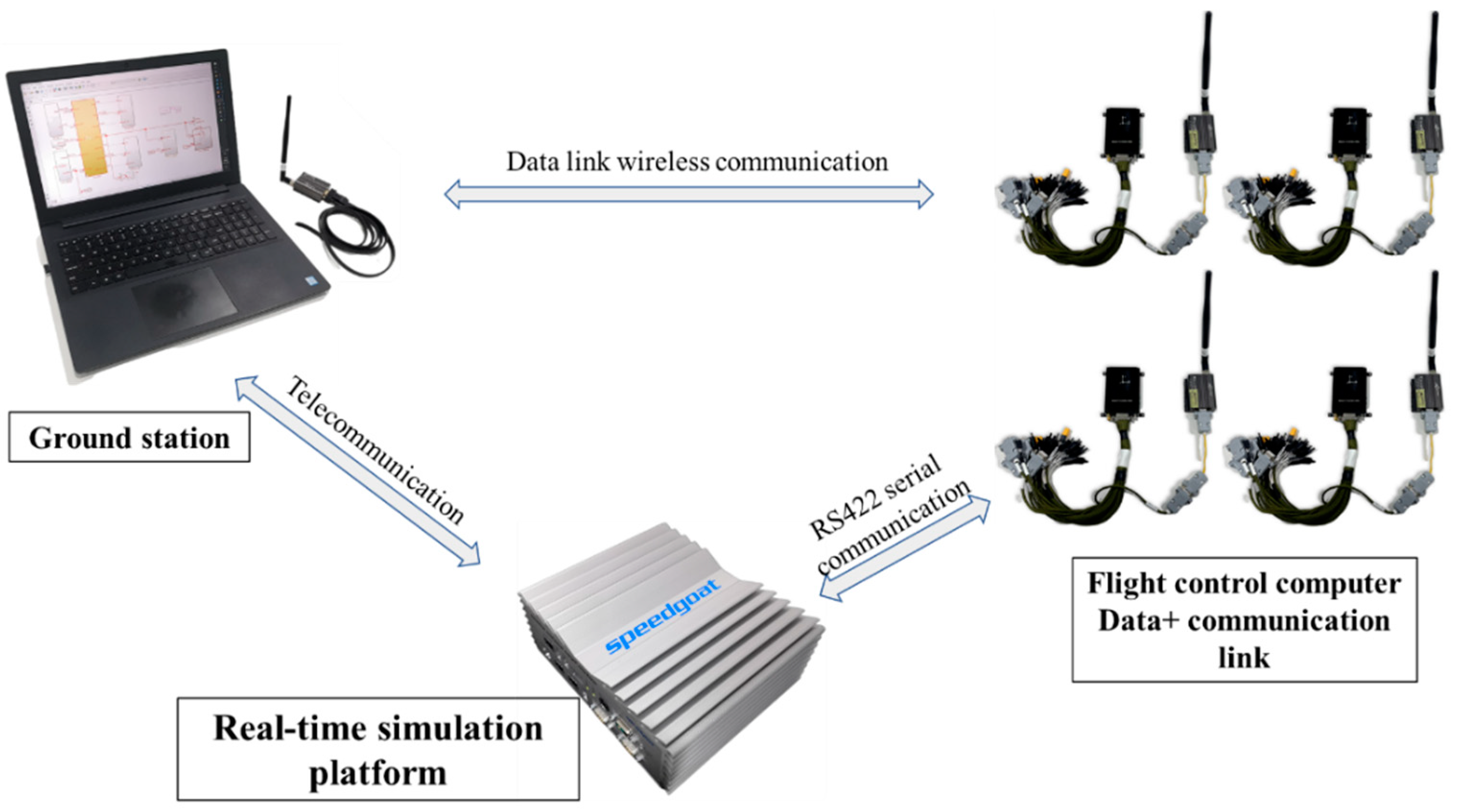
4.1.1. Simulation System Composition

The equipment connection relationship of the constructed semi-physical simulation system is shown in Figure 14. The simulation machine used the Speedgoat real-time simulation platform. The ground-station computer was responsible for starting the simulator, running the ground-station software, and establishing communication with the simulator through network protocols. The ground-station computer was connected to a communication node of the data communication link to establish wireless communication with all flight control computers participating in the simulation; communication between the simulator and the flight control computers was carried out through an RS422 serial port.

The flight control computer and the data communication links constituted the flight control system. We used four sets of flight control systems to simulate the formation of four aircraft. Each control system was connected to the Speedgoat real-time simulation system, receiving simulation data and controlling the dynamic model running in the simulator. The data communication links clicked the four sets of flight control computers with the ground-station computers for networking communication.

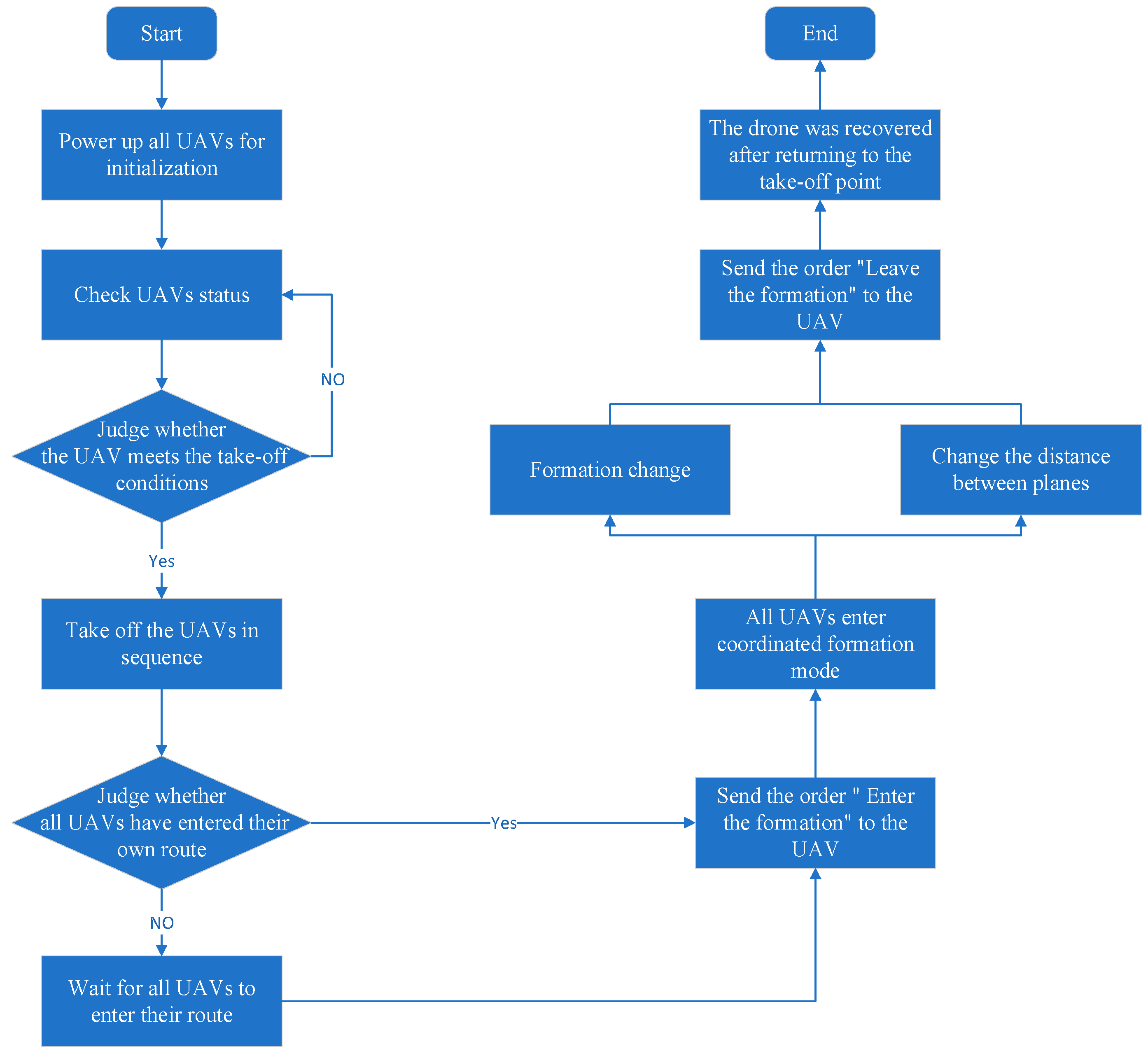
4.1.2. Semi-Physical Simulation Process

The goal is to simulate several scenarios in the flight of the UAVs. The initial stage of the semi-physical simulation involves starting the flight control system, connecting it to the ground station, and setting the flight control system to semi-physical simulation mode. The “Speedgoat” simulator is then started, and the aircraft model in the simulator begins to run and send data to the flight control computer. Finally, after the ground station confirms that the flight control computer system is operating normally, each UAV model takes off in turn before beginning the formation simulation verification procedure.

The process of the hardware-in-the-loop simulation is shown in Figure 15. The UAVs are lined up and turned on, and then wait for the flight control computer system to finish initializing. The ground station software monitors the state of the UAVs and launches those that fulfill the requirements. If the UAVs do not meet the take-off status, each unit is rechecked until the take-off conditions are met. When each UAV has entered the route and reached a suitable position, the command to fly in formation is sent to the UAVs through the ground station. The leader and followers join the multi-aircraft coordinated formation flight mode, which allows us to check the effect of collaborative formation flying. After entering the coordinated formation flight route, the formation change command can be delivered through the ground station. Simultaneously, the distance parameters among the followers in tight formations can be modified to fulfill diverse flight needs. The ground station delivers the instruction to “close the formation” when the formation test is complete, and each UAV begins to exit the coordinated formation mode in an orderly way. After leaving formation mode, the leader and followers fly along their routes before returning to the take-off spot to be recovered.

First set the initial speed of the leader and the follower as 20 m/s; the initial heading is north; the initial attitude angle is 0°; the initial altitude is 50 m; the initial position is any point; the maximum flight speed is 23 m/s, and the minimum flight speed is 17 m/s. Then the following three simulation scenarios are set up.

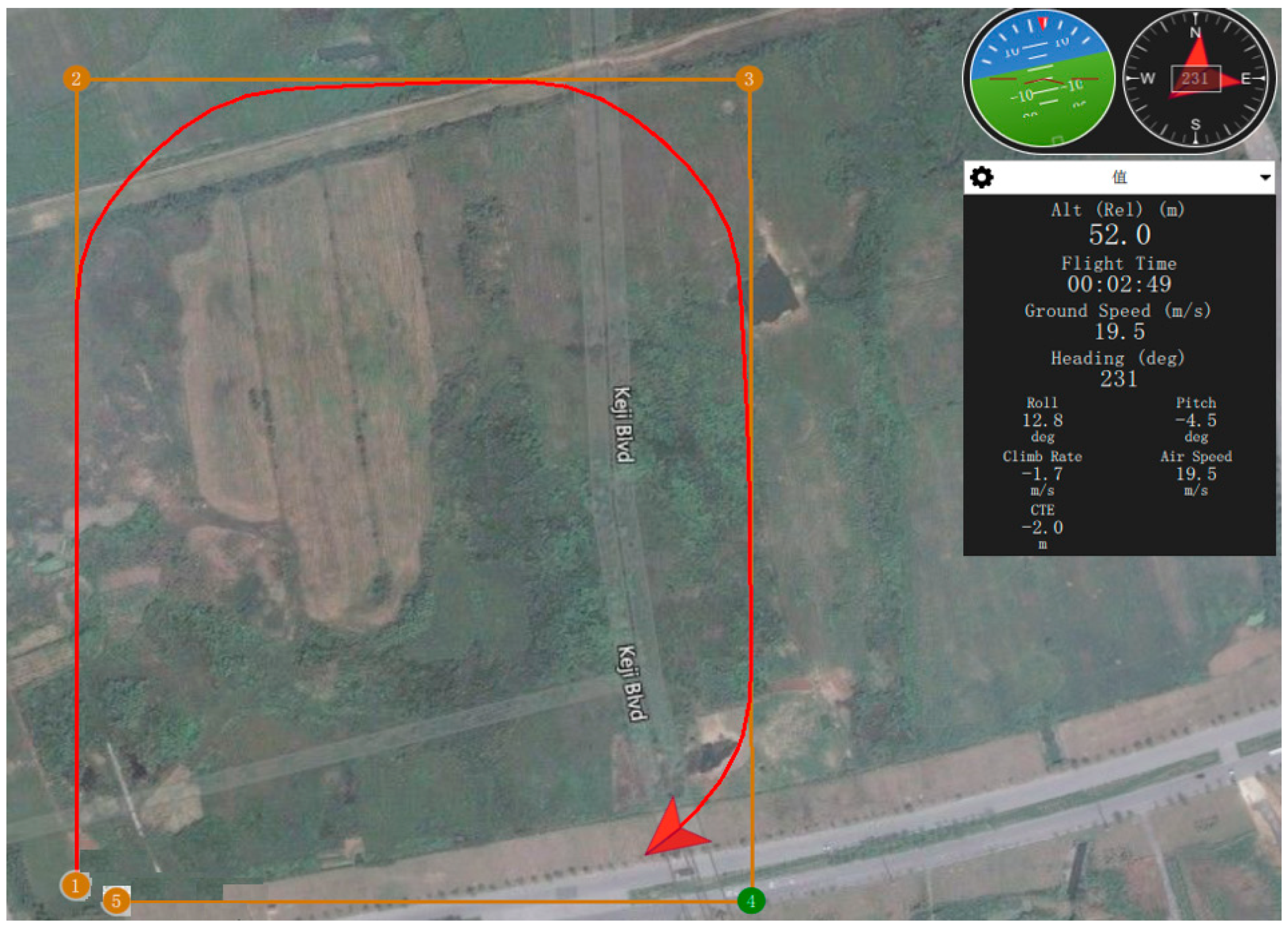
• Case 1: Waypoint flight simulation of the lead aircraft

As shown in Figure 16, there are five waypoints, waypoint 1 is the take-off point, and waypoint 5 is the landing point. The leader aircraft flies close to the route during straight flight, and while turning, it forms a smooth circular arc tangent to the route. This simulation demonstrates that the leader aircraft guidance law positively influences route tracking.

• Case 2: Flight simulation information mode

This simulation aims to model the flight conditions of several UAVs in cooperative formation mode. Two- and four-aircraft formations are considered in the hardware-in-the-loop simulations. The UAVs enter the fixed-wing state and begin the coordinated formation flight after they have all taken off. Each follower can fly in coordination with the leader at a fixed distance, as shown in Figure 17.

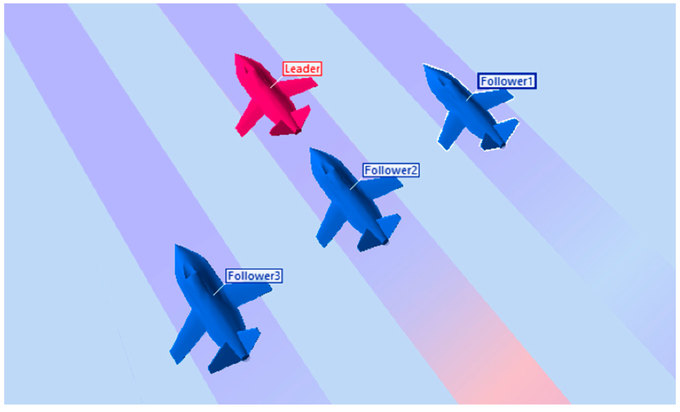
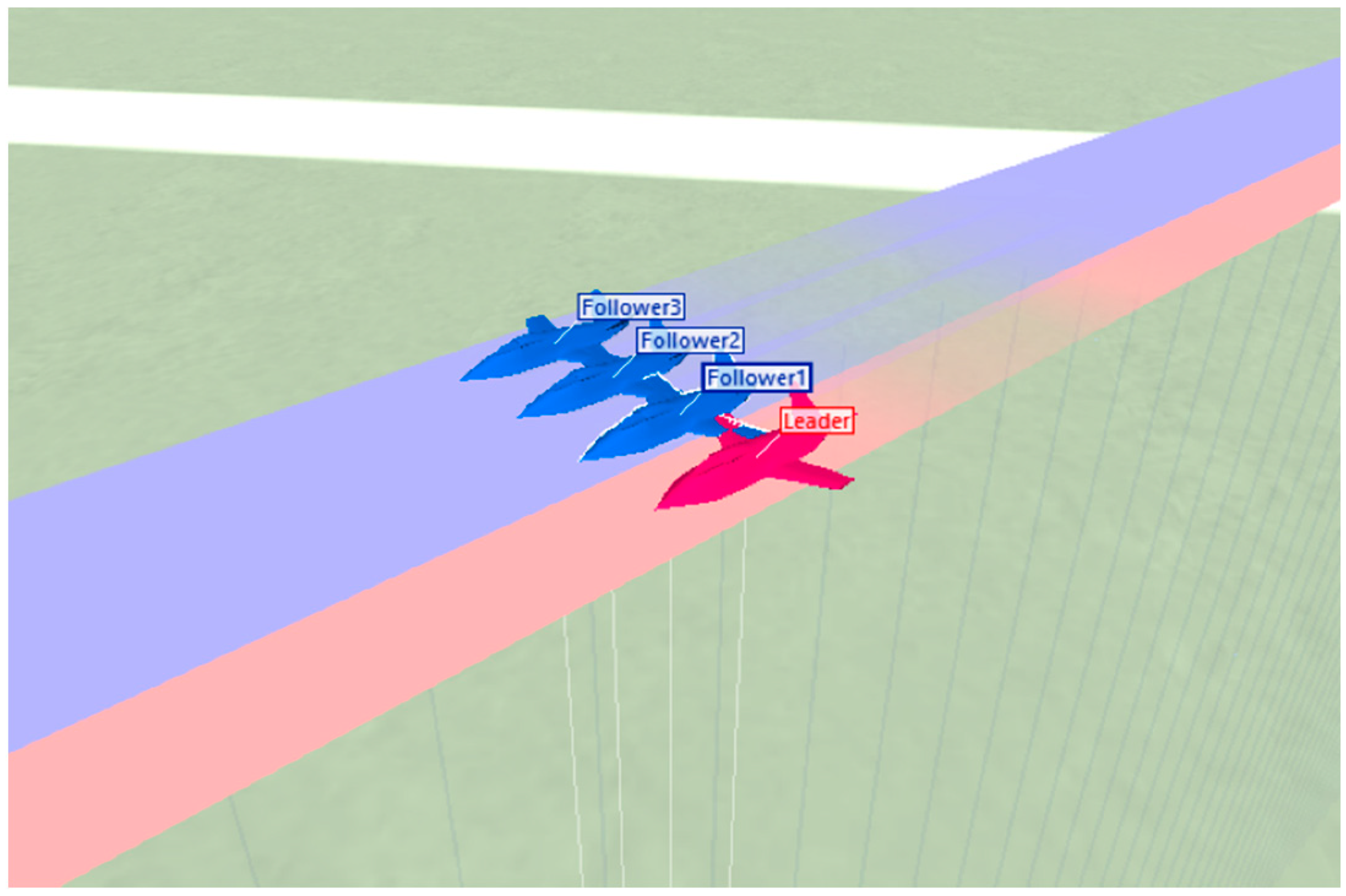
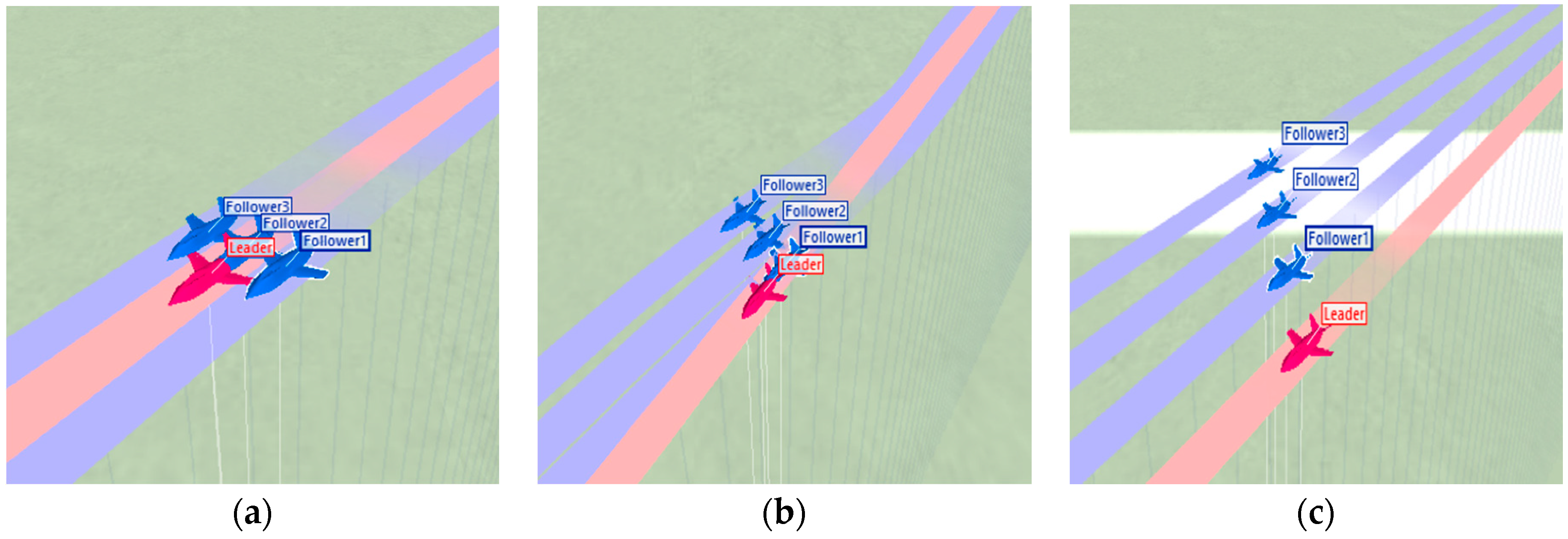
• Case 3: Formation transformation simulation

The ability to change formation is verified using the formation change simulation. First, the UAVs are controlled to form a stable shape, and then a command is sent from the ground station to modify the formation. The transformation from a four-aircraft triangle formation to a stepped formation demonstrates the transformation effect (see Figure 18).

The position changes in the formation change simulation are related to the formation before and after the change. As shown in Figure 19, the ordinate is the position difference between the follower and the leader when flying in shape. In the triangle formation, the three followers are behind the leader. Follower 2 is the closest to the leader and is directly behind the leader’s position; follower 1 and follower 3 are on either side of follower 2. In the stepped formation, the three followers are distributed on one side and fly at fixed distances. Figure 19 shows that the trajectory of position movement is relatively stable during the formation change process, the three followers can quickly reach their positions and there are no sudden jumps. Therefore, in the complex formation change process, the guidance law of the follower can guide the followers to follow the leader, which reflects the flexibility of the guidance law in the formation change.

The formation change simulation also verifies the response characteristics of the guidance law to changes in the guidance target, in which the critical parameter is the change of heading angle $\psi$. In this hardware-in-the-loop simulation experiment, the leader and followers have the same heading and fly parallel in the triangular formation. After receiving the formation change command, the formation management module generates a new route tracking point, and the guidance law directs the followers to the unique path tracking point, causing the heading angle to change. Figure 20 depicts the process of changing the formation’s heading angle. The heading angle of the followers changes rapidly after receiving the command to change formation, and the heading rise in the followers quickly converges once the formation change is completed. This shows that the heading angle of the follower can quickly respond to the change of the virtual dynamic point and converge to the target heading angle.

4.2. Results of Real Flight Test

This experiment used two types of coordinated formation flight: stepped formation and linear formation. The UAVs can easily create these two formations, and they provide a good test of the formation maintenance and transformation control methods proposed in this paper. Coordinated flight in a linear formation was initially carried out. The ground station then sent a command to create a ladder formation to each UAV, and the formation changed to a stepped formation and continued to fly. Figure 21 shows the actual flight conditions of the linear and stepped collaborative formations.

4.3. Flight Data Analysis

The core component of this study is the guidance law algorithm. The index for evaluating the effect of the guidance law is the tracking effect of the followers’ heading angle $\psi$ after changing the guidance target. Figure 22 shows that when the leader’s heading angle changed, the followers’ steering angles responded in time and tracked the new heading, demonstrating that the guidance law algorithm satisfies the real-time requirements and verifying the response characteristics of the guidance law proposed in this paper.

The flight trajectories of each UAV can intuitively show the effect of the collaborative formation. The three-dimensional trajectories of the actual flight route derived from the stable formation are shown in Figure 23a. Longitude, latitude, and height are the three geographic coordinate values that make up the trajectory. Latitude and longitude are horizontal coordinates, while height is the vertical coordinate. The diagram shows that each UAV maintains a set distance and cooperates to fly within the permissible error range. Figure 23b shows the entire formation trajectory, which intuitively reflects the flying effect of the trajectory in the real scene. On the whole, the formation can maintain a safe distance to fly in a straight line. At the turn, the follower can respond in time and follow the leader.

In analyzing the flight data, it was discovered that the position error did not strictly converge, indicating that the formation control accuracy can still be improved. The following two factors are the primary causes of coordinated formation flight errors: (1) the issue of reliably measuring wind disturbances has not been addressed in this paper, so the impact of wind disturbances on the flight is not estimated. Therefore, the leader and the followers use the guidance and control laws without considering the effects of wind during the actual flight; (2) due to the wireless data link used during the actual flight, the UAVs have a communication delay. However, the communication delay was not considered when designing the control laws, resulting in a minor time difference between the cooperative information received by the followers and the information given by the leader.

In summary, this study has investigated the coordinated formation control of fixed-wing UAVs, combined with current engineering practice and a specified acceptable range of control error. The actual flight effect satisfies the design specifications and can meet the formation control needs of specific activities.

5. Conclusions

The research goal was the control of fixed-wing UAVs in cooperative flight formation, including the design and simulation of a formation guidance algorithm, formation management, and formation transformation. The design of a collaborative guidance law is based on the classic missile-type parallel-approach method. The guidance law was designed for three guidance modes: straight line, turning, and circling, which increases the flexibility of formation changes in the form of tracking target virtual points. The main research contributions are as follows:

• Commonly used guidance laws were studied, and the characteristics of each rule were compared and analyzed. Finally, the parallel approach method was chosen as the guidance law. The parallel approach method itself has no concept of bandwidth in theory, it is a geometric expression. Since there is no integral controller, there must be an error, which is caused by the control bandwidth of the inner loop, but it must converge at low frequencies and converge to zero. The advantage of using the parallel approach method for formations is that since the position is known, there is no need to observe the line-of-sight angular velocity, and there is no observer or differentiator argument. The accuracy and refresh rate of the observed position and velocity is much higher than that of hitting an unknown target through the seeker. A formation management method based on cooperative waypoint tracking was proposed, and several common formations were given as examples. The method of harmonious formation transformation will be considered in future studies.
• The MATLAB/Simulink simulation platform was used to model and simulate the designed cooperative formation control algorithm. Hardware-in-the-loop simulations and actual flight tests have demonstrated the practicality of the collaborative formation guidance algorithm. The control algorithm developed in this paper can also perform specific formation tasks. It is worth mentioning that the parallel approach method in the flight test is mainly applied to the follower tracking the lead vehicle, but the idea of tracking the virtual target point can also be applied to the lead vehicle tracking the reference route.
• Using the parallel approach method as the guidance method of the leader-follower mode not only increases the flexibility of the formation reorganization, but also can be applied to the formation guidance of high-speed vehicle.

References

1. Gai, W.; Zhang, N.; Zhang, J.; Li, Y. A constant guidance law-based collision avoidance for unmanned aerial vehicles. Proc. Inst. Mech. Eng. Part G J. Aerosp. Eng. 2018, 233, 1204–1216. [Google Scholar] [CrossRef]
2. No, T.S.; Kim, Y.; Tahk, M.-J.; Jeon, G.-E. Cascade-type guidance law design for multiple-UAV formation keeping. Aerosp. Sci. Technol. 2011, 15, 431–439. [Google Scholar] [CrossRef]
3. Sullivan, J.M. Evolution or revolution? The rise of UAVs. IEEE Technol. Soc. Mag. 2006, 25, 43–49. [Google Scholar] [CrossRef]
4. Sanders, R. An Israeli Military Innovation: UAVs. JFQ Jt. Force Q. 2002, 33, 114–118. [Google Scholar]
5. Isby, D.C. Us military vtol uavs. Air Int. 2016, 91, 22. [Google Scholar]
6. Fan, Q.J.; Yang, Z.; Fang, T.; Shen, C. Research Status of Coordinated Formation Flight Control for Multi-UAVs. Acta Aeronaut. Astronaut. Sin. 2009, 30, 683–691. [Google Scholar]
7. Xu, Z.D.; Shang, T.; Sun, R.M.; Wang, D.M. A Virtual Environment for Simulation of Formation Flight. Appl. Mech. Mater. 2015, 713–715, 263–266. [Google Scholar] [CrossRef]
8. Joongbo, S.; Chaeik, A.; Youdan, K. Controller design for uav formation flight using consensus based decentralized approach. In Proceedings of the Aerospace Conference, Seattle, WA, USA, 6–9 September 2009. [Google Scholar]
9. Linorman, N.; Liu, H. Formation UAV flight control using virtual structure and motion synchronization. In Proceedings of the American Control Conference (ACC), Seattle, WA, USA, 11–13 June 2008. [Google Scholar]
10. Zhang, J.M.; Qing, L.I.; Cheng, N.; Liang, B. Nonlinear path-following method for fixed-wing unmanned aerial vehicles. J. Zhejiang Univ. Sci. C Comput. Electron. 2013, 14, 125–132. [Google Scholar] [CrossRef]
11. Zhang, M.; Xia, W.; Huang, K.; Chen, X. Guidance law for cooperative tracking of a ground target based on leader-follower formation of UAVs. Acta Aeronaut. Astronaut. Sin. 2018, 39, 230–242. [Google Scholar]
12. Park, C.; Kim, Y. Real-time leader-follower UAV formation flight based on modified nonlinear guidance. In Proceedings of the 29th Congress of the International Council of the Aeronautical Sciences (ICAS), Saint Petersburg, Russia, 7–12 September 2014. [Google Scholar]
13. Wang, Y.; Shan, M.; Wang, D. Motion Capability Analysis for Multiple Fixed-Wing UAV Formations with Speed and Heading Rate Constraints. IEEE Trans. Control. Netw. Syst. 2019, 7, 977–989. [Google Scholar] [CrossRef]
14. Kalra, A.; Anavatti, S.; Padhi, R. Aggressive Formation Flying of Fixed-Wing UAVs with Differential Geometric Guidance. Un. Syst. 2017, 5, 97–113. [Google Scholar] [CrossRef]
15. Oh, Y.S.; Park, J.H.; Kim, J.H.; Huh, U.Y. Obstacle Avoidance of Leader-Follower Formation. Trans. Korean Inst. Electr. Eng. 2011, 60, 1761. [Google Scholar] [CrossRef] [Green Version]
16. Lee, D.; Kim, S.-K.; Suk, J. Design of a Track Guidance Algorithm for Formation Flight of UAVs. In Proceedings of the AIAA Guidance, Navigation, and Control Conference, Grapevine, TX, USA, 9–13 January 2017; pp. 469–482. [Google Scholar]
17. Wang, X. A Cooperative Guidance Law for UAVs Target Tracking. WSEAS Trans. Syst. 2021, 19, 324–335. [Google Scholar] [CrossRef]
18. Wang, S.; Wei, R.; Guo, Q.; Wei, W. UAV Guidance Law for Coordinated Standoff Target Tracking. Hangkong Xuebao Acta Aeronaut. Astronaut. Sin. 2014, 35, 1684–1693. [Google Scholar]
19. Zipfel, P.H. Aerodynamic symmetry of aircraft and guided missiles. J. Aircr. 1976, 13, 470–475. [Google Scholar] [CrossRef]
20. Feng, Q.D.; Pei, H.L. The Design of Hardware-in-the-loop Simulation for UAV. Fire Control Command Control 2011, 36, 166–168. [Google Scholar]
21. Sun, J.; Li, B.; Wen, C.Y.; Chen, C.K. Design and implementation of a real-time hardware-in-the-loop testing platform for a dual-rotor tail-sitter unmanned aerial vehicle. Mechatronics 2018, 56, 1–15. [Google Scholar] [CrossRef]
Figure 1. Lateral movement of the leader-follower formation.
Aerospace 09 00272 g001
Figure 2. Vertical motion of the leader–follower formation model.
Aerospace 09 00272 g002
Figure 3. Linear guidance.
Aerospace 09 00272 g003
Figure 4. Linear guide in vertical direction.
Aerospace 09 00272 g004
Figure 5. Relationship between flight path and waypoint in turn guidance mode.
Aerospace 09 00272 g005
Figure 6. Turn navigation (clockwise turn).
Aerospace 09 00272 g006
Figure 7. Hovering mode in actual flight.
Aerospace 09 00272 g007
Figure 8. Hover guidance.
Aerospace 09 00272 g008
Figure 9. Virtual dynamic tracking point calculation.
Aerospace 09 00272 g009
Figure 10. Kinematic relationship between follower and dynamic tracking point.
Aerospace 09 00272 g010
Figure 11. Follower heading control command tracking effect.
Aerospace 09 00272 g011
Figure 12. Formation simulation.
Aerospace 09 00272 g012
Figure 13. Relative distance between leader and followers.
Aerospace 09 00272 g013
Figure 14. Device connection diagram for hardware-in-the-loop simulation.
Aerospace 09 00272 g014
Figure 15. Formation flight test flowchart.
Aerospace 09 00272 g015
Figure 16. Semi-physical simulation of the lead aircraft tracking waypoints.
Aerospace 09 00272 g016
Figure 17. Hardware-in-the-loop simulation.
Aerospace 09 00272 g017
Figure 18. Semi-physical simulation of formation transformation: (a) triangular formation; (b) intermediate state of formation change; (c) ladder formation.
Aerospace 09 00272 g018
Figure 19. Position of the followers relative to the leader during the formation change.
Aerospace 09 00272 g019
Figure 20. Heading angle information change.
Aerospace 09 00272 g020
Figure 21. Actual flight diagram of the four-machine coordinated formation: (a) linear formation; (b) ladder formation.
Aerospace 09 00272 g021
Figure 22. Control effect of the actual flight heading channel of the four aircraft in cooperative formation.
Aerospace 09 00272 g022
Figure 23. Actual flight route of the four-plane cooperative formation: (a) straight trajectory; (b) flight trajectory.
Aerospace 09 00272 g023