Article

Geostationary Orbital Debris Collision Hazard after a Collision

1
Department of Aerospace Science and Technology, Space Engineering University, Beijing 101416, China
2
China Jiuquan Satellite Launch Centre, Jiuquan 735000, China
*
Author to whom correspondence should be addressed.
Aerospace 2022, 9(5), 258; https://doi.org/10.3390/aerospace9050258
Submission received: 13 February 2022 / Revised: 23 April 2022 / Accepted: 9 May 2022 / Published: 10 May 2022
(This article belongs to the Special Issue Space Debris Removal: Challenges and Opportunities)

Abstract

:
Many space objects are densely distributed in the geostationary (GEO) band, and the long-term impact of the collision of GEO spacecraft and space debris on the GEO environment has attracted more and more attention. After summarizing the advantages and disadvantages of the long-term evolution model based on the “Cube” collision probability calculation model, the “Grid” model, a long-term evolution model especially suitable for GEO band, was established. For four types of collision and disintegration events, the “Grid” model was used to study the space environment in the GEO band after collisions between GEO spacecraft and space debris. Future collisions were simulated, and the number of space objects in the next 100 years was counted. Once space debris and massive spacecraft were completely disintegrated after collision, the number of space objects and the collision probability increased sharply, and this caused a collision cascading syndrome. Even if there was no initial disintegration event, collision and disintegration events occurred in the long-term evolution of the GEO band, which led to an increase in the number of space objects. However, the collision probability was much lower, and the number of space objects grew much more slowly without the initial collision.

1. Introduction

With space launch activities, the number of space objects is increasing day by day, especially in the geostationary (GEO) band, which is of great significance to communication and navigation. There, the distribution of space objects is denser, and a large number of spacecraft exist in a colocated manner [1,2,3]. As of the end of 2020, in a range of about 200 km from GEO in height, the number of space objects within 15° of latitude on both sides of the equator exceeded 3500 [4,5,6]. As more and more spacecraft enter outer space, the problem of spacecraft collision has become increasingly prominent [7,8,9,10]. The long-term impact of the debris generated by the collision of GEO spacecraft with space debris on the space environment of GEO has become a problem of increasing concern [11,12,13].
For space environment problems, many countries and institutions have established long-term evolution models, mainly including: the LEO (Low Earth Orbit)-to-GEO Environment Debris (LEGEND) model and EVOLVE model of National Aeronautics and Space Administration (NASA) [14,15,16], the Meteoroid and Space Debris Terrestrial Environment Reference (MASTER) of European Space Agency (ESA) [17], the Debris Analysis and Monitoring Architecture for the Geosynchronous Environment (DAMAGE) and Integrated Debris Evolution Suite (IDES) of Britain [18,19], the Space Debris Mitigation long-term analysis program (SDM) of Italy [20], Modelling the Evolution of Debris in the Earth’s Environment (MEDEE) of France [21], and the Long-Term Utility for Collision Analysis (LUCA) of Germany [22]. Since the prediction of future collision is random, the Monte Carlo stochastic algorithm has been employed to predict future events [23]. The “Cube” collision probability calculation model was employed in the DAMAGE and LEGEND models [24,25]. The space is divided into discrete units from three dimensions of geocentric distance, right ascension, and declination. It is assumed that the motion of space objects in the discrete units is like that of gas molecules, and the collisions in each discrete unit are studied. However, the deficiency of the “Cube” model is that the prediction of the position of the space objects according to the motion characteristics of gas molecules does not conform to orbital dynamics. Zhang Binbin from the National University of Defense Technology established a layered discretization model for the macroscopic quantity of space density in the near-Earth space. The space environment for the next 200 years was predicted. The long-term evolution and distribution characteristics of the debris cloud, the hazard of collision of large spacecraft with space debris, and the impact of the large satellite constellations on the space environment were studied [26].
On the space environment problem of GEO, [27] analyzed the diffusion of newly generated space debris after the collision between GEO spacecraft and space debris. Space debris spread to the entire GEO region in about half a day, posing a greater threat to spacecraft in GEO band. Ref. [28] analyzed the collision hazard of newly generated debris to GEO spacecraft within 3 days after the collision of a GEO spacecraft with space debris without the support of ground observation data.
On the space environment problem after the collision of GEO spacecraft with space debris, the advantages and disadvantages of long-term evolution models were investigated [29]. Based on the “Cube” collision probability calculation model, the current paper improved its deficiencies in describing the motion characteristics of space objects and established the “Grid” model, a model especially suitable for long-term evolution analysis of space objects in the GEO band. The “Grid” model was used to simulate the long-term evolution of the space environment in the GEO band after a GEO spacecraft collides with space debris. For four types of collision events, the model was used to study the space environment in the GEO band in the next 100 years and obtain the long-term diffusion characteristics of space debris and the growth in the amount of space debris in the GEO band.
The remaining parts of the paper are organized as follows. Section 2 presents the collision hazard analysis and modelling. Section 3 presents a simulation the GEO space environment after a collision between GEO spacecraft and space debris and provides a description of the experimental results. Section 4 is the conclusion.

2. Collision Hazard Analysis and Modelling

When calculating the collision probability of space objects, if the collision probability between any pair of space objects is calculated at each time step, the time complexity is ( N ! t s t e p ) , where N is the number of space objects, t is the time span, and step is the time step of the numerical integration used for the orbital long-term propagation. Obviously, there is a huge amount of calculation in practice, especially when t is large and the feasibility is poor. The space is discretized and divided into m independent units. Assuming that collisions occur only in discrete units, the time complexity of the calculation will be reduced to ( ( N m ) ! N t s t e p ) . Therefore, the GEO space is first discretized, then the collision probability between space objects in each unit is calculated, and then a space environment analysis model is established to simulate the space environment in the future.

2.1. GEO Band Discretization

The GEO band ranges within 200 km from GEO in height and 15° of latitude on both sides of the equator. The GEO band is discretized from two dimensions of right ascension λ and declination δ . The volume unit is defined as:
V i j = { ( r , λ , δ ) | | r a s | 100   km , | λ λ i | λ 2 , | δ δ i | δ 2 , | δ | 15 ° }
where a s = 42,165.8 km is the GEO nominal orbital semi-major axis, δ = λ = 0.5 ° .To simplify the calculation of the collision probability between space objects, the following assumptions are made:
first, for any two space objects, collisions may occur only when the two space objects are in a volume unit at the same time;
second, in a volume unit, collisions occur between only two space objects, and there is no simultaneous collision of more than two;
third, the center of mass of each space object coincides with the center of its circumscribed envelope sphere;
fourth, since the collision of two space objects lasts for a very short time, the uncertainty of the velocity vector during the collision is ignored.
Under the above assumptions, the space objects collision problem in the GEO band is transformed into a collision problem within each independent volume unit.

2.2. Collision Probability of Space Objects within the Volume Unit

For two space objects E and P in a volume unit, their circumscribed envelope sphere radii, position vectors, and velocity vectors are defined as R E , R P ; r E , r P ; and v E , v P , respectively. Then the sum of the radius, the relative position vector, and the relative velocity vector are as follows:
R 0 = R E + R P
r = r P r E
v = v P v E
When the distance between the two space objects is less than the sum of the radius of the circumscribed envelope sphere, that is, | r | R 0 , the two space objects collide. The right-handed coordinate system is centered at the center of mass of E. Taking the center of mass of E as the center of the sphere, and taking R 0 as the radius, the spherical surface is the collision sphere, denoted as S. The inflow velocity scalar v n is the velocity of the space object P entering the collision ball, and the outflow velocity scalar v n + is:
v n = { v r n , v r n < 0 0 , v r n 0
v n + = { v r n , v r n > 0 0 , v r n 0
where n is the outer normal vector of the collision sphere surface S. The inflow probability P and the outflow probability P + in the time period ( t 1 , t ) are as follows:
P = t 1 t d t S f ( r ) v n d s
P + = t 1 t d t S f ( r ) v n + d s
where f ( r ) is the probability density function of the relative position vector in space. The inflow probability and outflow probability per unit time at t are:
p t ( t ) = d P d t = S f ( r ) v n d s
p t + ( t ) = d P + d t = S f ( r ) v n + d s
where p t ( t ) is the probability of collision between E and P in unit time at time t. Since the space objects E and P obey the three-dimensional Gaussian distribution, the expectation of E is μ E = r E , and the covariance matrix of E is C E . The expectation of P is μ P = r P , and the covariance matrix of P is C P . Since E and P are independent of each other, r obeys a three-dimensional Gaussian distribution, and its expectation and covariance are:
μ r = r P r E
C r = C P + C E
According to the Gauss formula:
V i j f ( r ) d v = S f ( r ) v n d s S f ( r ) v n + d s = P t P t +
The probability that the space object P flows out of the collision ball is 0, that is, P + = 0 . The collision probability of E and P per unit time at time t is:
P t = P t = V i j f ( r ) d v
According to the collision probability calculation method in [28], the collision probability of two space objects in unit time at time t is obtained:
P t = exp [ r t 2 4 σ 2 ] [ 1 exp ( R 0 2 4 σ 2 ) ]
The collision probability at the time t = t k + 1 is the average collision probability in the time [ t k , t k + 1 ] . The product of the collision probability at this moment and the length of the time interval is the collision probability in this period. The expectation of collisions at the time step [ t k , t k + 1 ] is the sum of the product of the collision probability and the time interval in each volume unit, namely:
E ( P t k t k + 1 ) = i , j > i N t k t k + 1 P t ( i , j ) d t = λ , δ i , j > i N λ , δ P t ( i , j ) ( t k + 1 t k )
where, P t ( i , j ) is the collision probability of two space objects in the same volume unit at time t = t k + 1 .

2.3. Collision Hazard Analysis Steps

According to the characteristics of the GEO orbit, a long-term evolution and collision analysis model of space debris especially suitable for the GEO band, the “Grid” model, was established. The “NASA Standard Breakup Model” was employed as the collision disintegration model in the “Grid” model [30]. The semianalytical perturbation solution of the averaged Kepler orbital elements given by Kozai’s perturbation method was employed as the orbit propagation model [31,32]. Future launches and space debris removal strategies were not considered. The steps of the “Grid” model are:
first, the GEO area is divided into grids from two dimensions, right ascension and declination, as stated in Section 2.1;
second, the semianalytical orbit model is used to propagate the orbit of space objects with a time step of 24 h;
third, the collision probability of space objects in each grid at the current time step is calculated, as stated in Section 2.2;
fourth, a randomly generated number is used to determine whether a collision has occurred between any two space objects in each volume unit. A random number F between (0, 1) is generated. If F < P, the two space objects collide in the volume unit at the moment. Otherwise, there is no collision;
fifth, if a collision occurs, the space object pool is updated to perform collision probability calculation, collision prediction, and collision simulation for the next time step. If no collision occurs, the collision probability calculation, collision prediction, and collision simulation of the next time step are directly continued.

3. Simulation and Results

Space debris from the Molniya orbit and the GEO band were selected to collide with the spacecraft AMC-2. Launched from Guiana Space Center in 1997, AMC-2 is a commercial communications satellite of the United States. The NORAD (North American Aerospace Defense Command) ID of AMC-2 is 24,713, and the mass of AMC-2 is 2648 kg. AMC-2 is located above 100.98° W longitude. The energy ratio was defined as:
E P = m p v 2 2 m t
The threshold energy ratio was defined as EP = 40 kJ/kg. According to NASA Standard Breakup Model [29,33], if E P < E P , the space objects will be incompletely disintegrated. If E P > E P , the space objects will be completely disintegrated. The disintegration mass was defined as:
m t o t = { m t + m p , E P E P m p v 2 [ km / s ] 2 , E P < E P
According to the method of [27], the collision velocities of space debris from Molniya orbit and the GEO band with the spacecraft were 2980.6 m/s and 802.6 m/s, respectively. Therefore, if the mass of space debris from the Molniya orbit were greater than 23.8 kg, the two space objects would completely disintegrate, and if its mass were less than 23.8 kg, they would incompletely disintegrate. If the mass of space debris from the GEO band were greater than 328.9 kg, the two space objects would completely disintegrate, and if its mass were less than 328.9 kg, they would incompletely disintegrate. The complete and incomplete disintegration of the two types of debris and the GEO spacecraft were simulated, as shown in Table 1.
The initial GEO population, including the classical orbital elements, was obtained through space track [34]. The number of initial space objects was 1511. With the “Grid” model, long-term evolution analysis was carried out. The GEO band was divided into grids every 0.5°. (−15°, 15°) declination was divided into i = 1, 2, …, 60 layers; the i-th layer represented declination [ 15 + 0.5 ( i 1 ) , 15 + 0.5 i ] ° . The right ascension was divided into j = 1, 2, …, 720 layers, and the j-th layer represented [ 0.5 ( j 1 ) , 0.5 j ] ° . (j, i) referred to:
V i j = { ( r , λ , δ ) | | r a s | 100 km , [ 0.5 ( j 1 ) ] ° < λ < ( 0.5 j ) ° , [ 15 + 0.5 ( i 1 ) ] ° < δ < ( 15 + 0.5 i ) ° }
A timestep of 86,400 s was taken to analyze the number of collisions in the next 100 years, and the growth in the total number of space objects in or passing through the GEO band with size greater than 0.05 m was studied. In the collision analysis, only collisions between space objects with sizes larger than 0.05 m were analyzed; the influence of space debris with size smaller than 0.05 m was ignored. Future launch activities and debris removal were ignored. Since the Monte Carlo simulation was used for the prediction of collision events, the results of each simulation were uncertain. Therefore, for each scenario, 20 independent repetitions of the simulation were conducted.

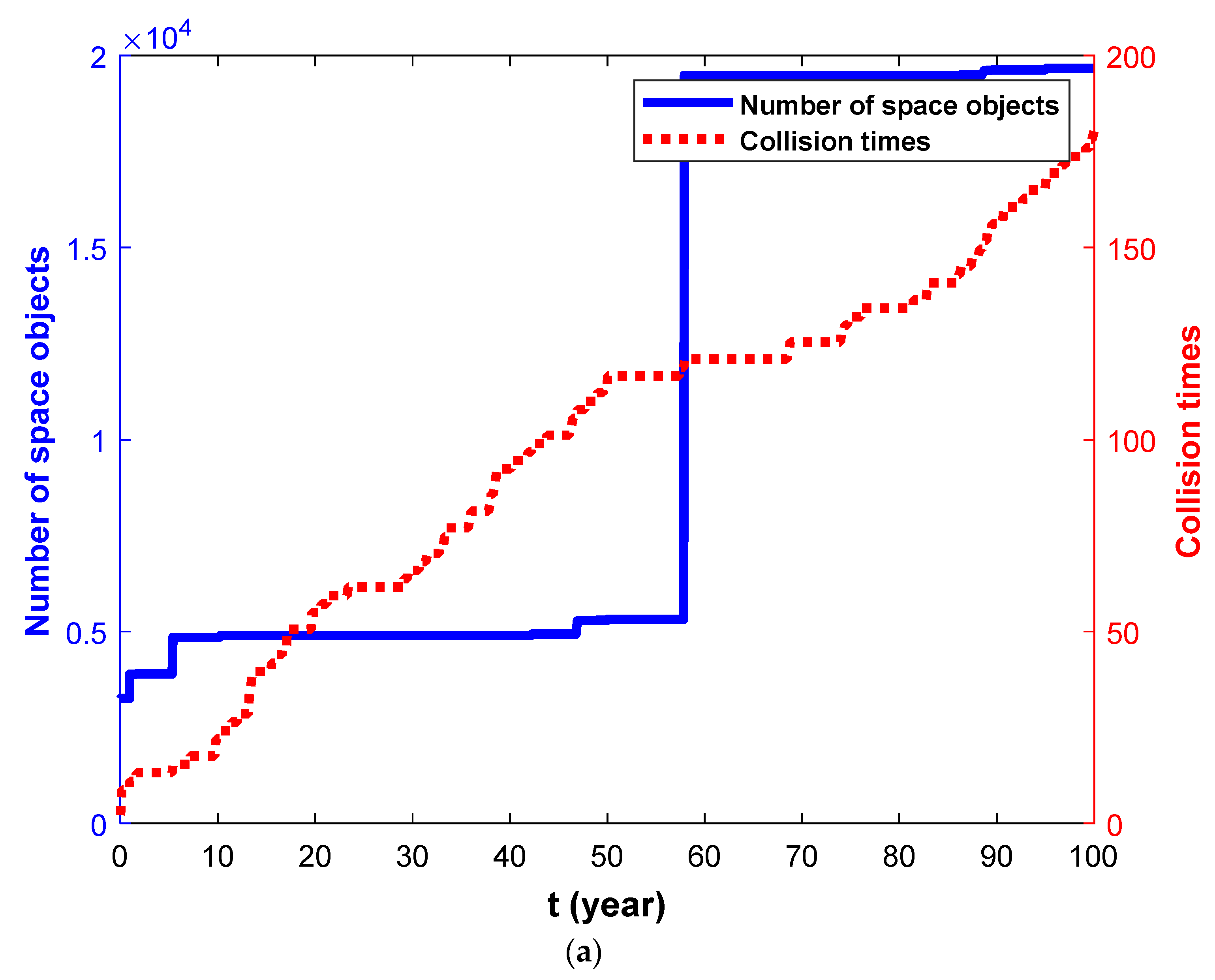
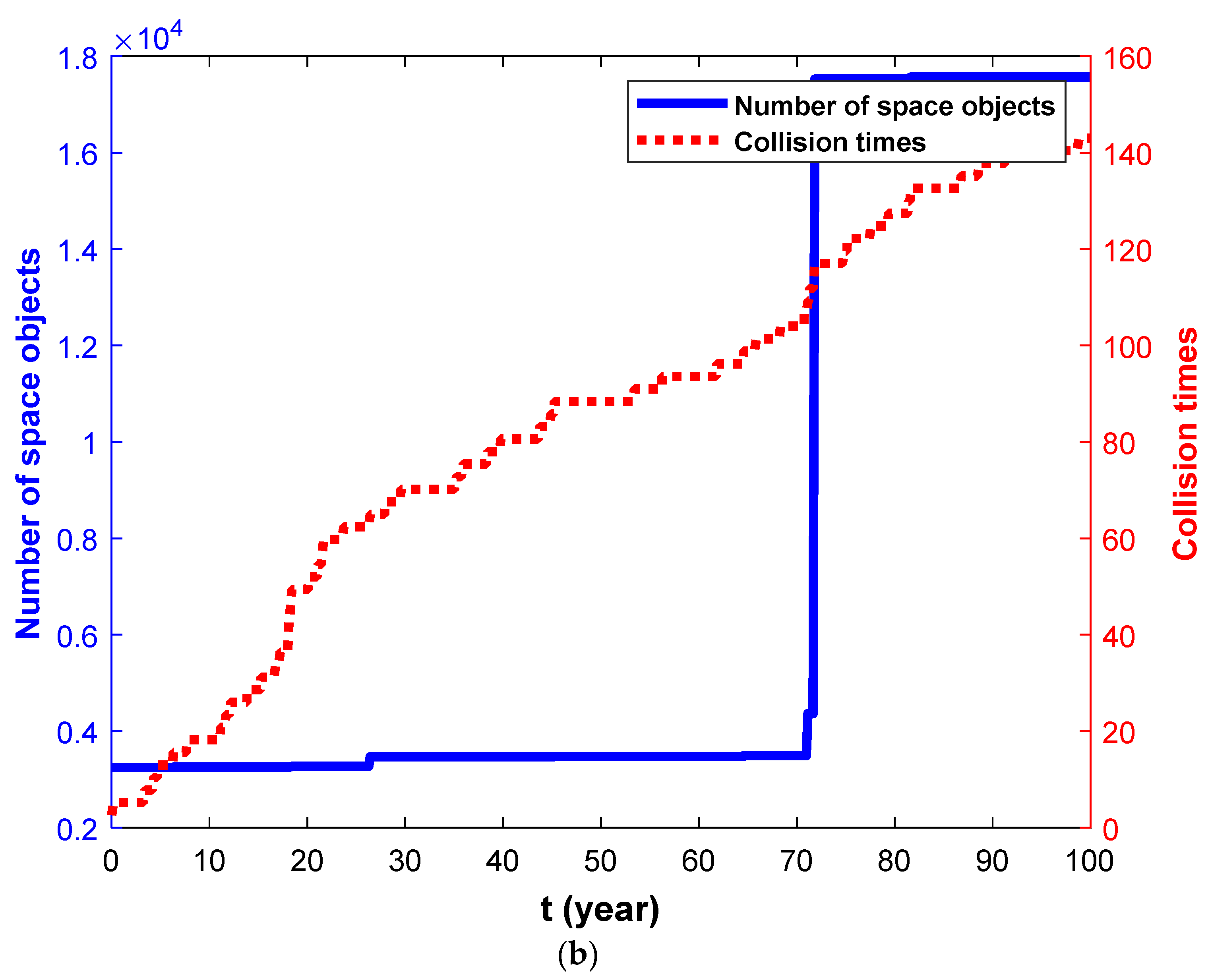
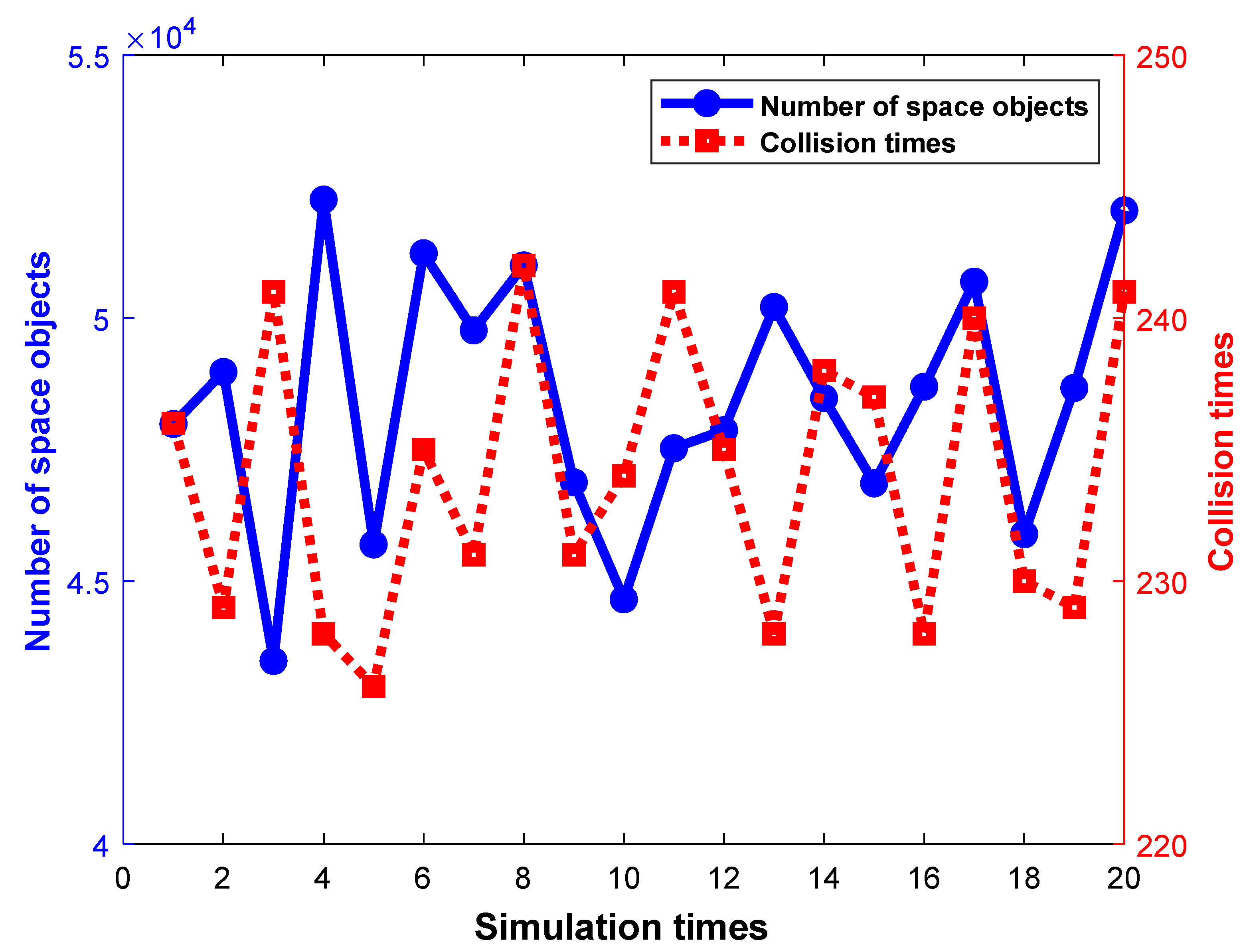
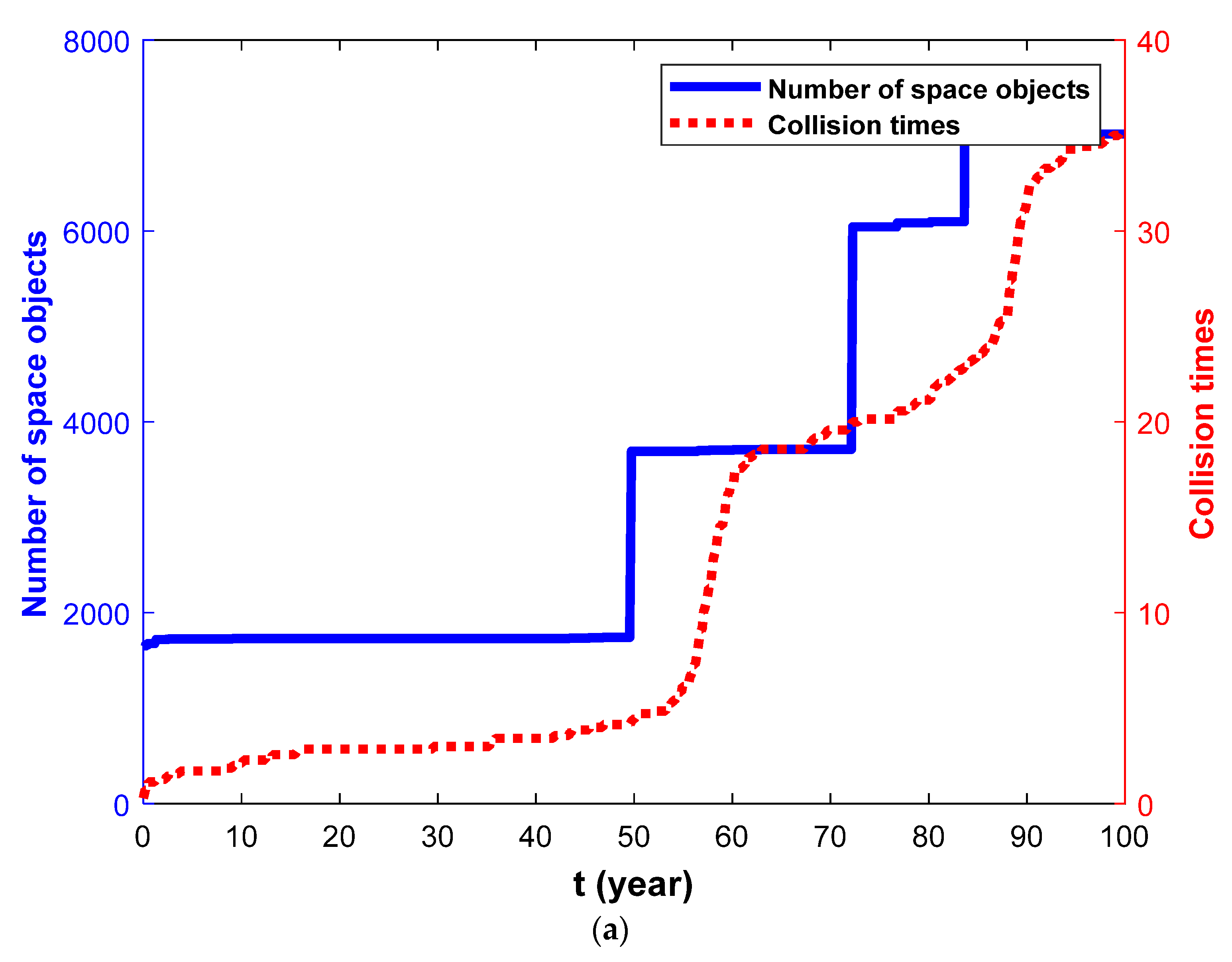
3.1. Complete Disintegration Simulation

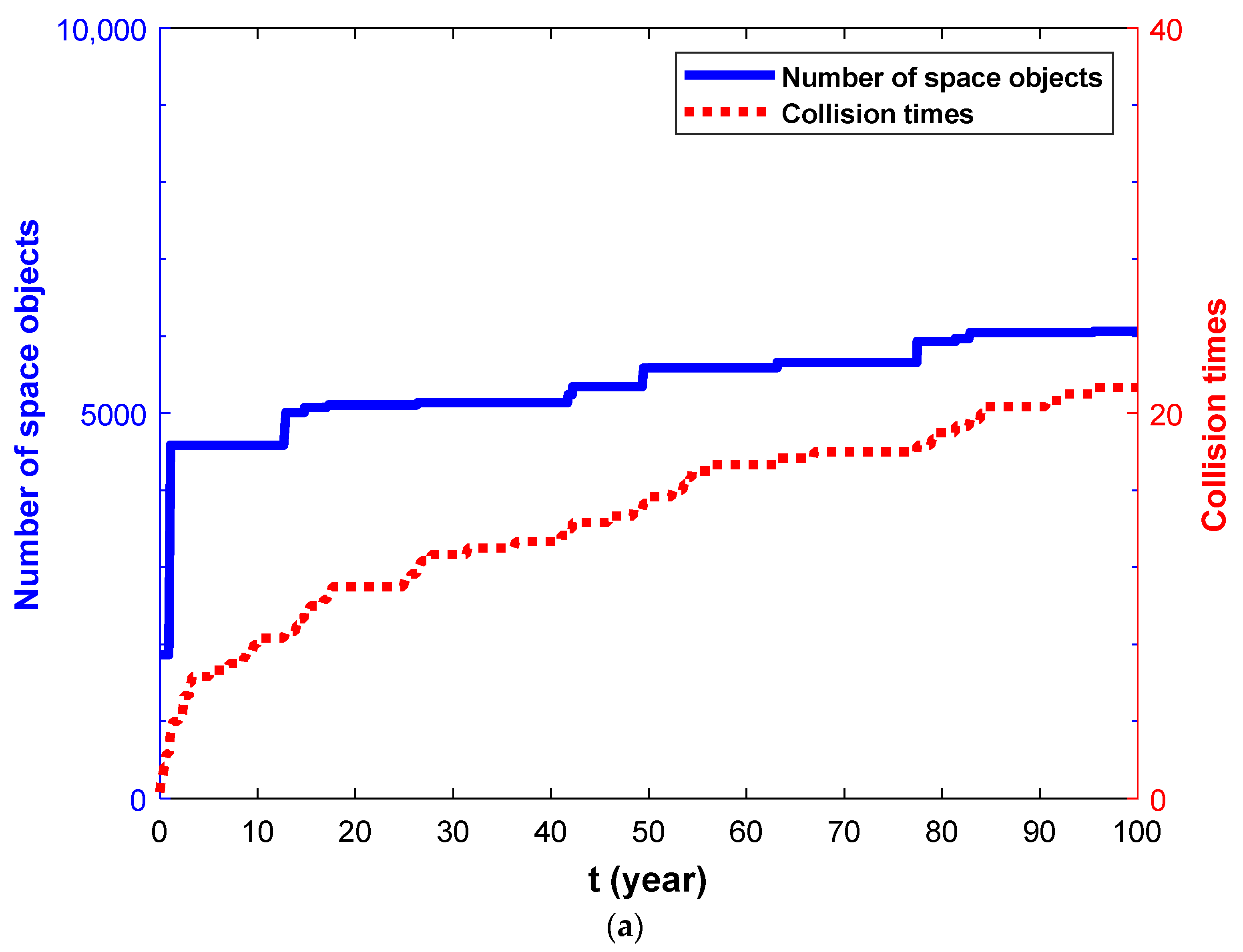
3.1.1. Scenario No. 1

In scenario No. 1, AMC-2 collided with space debris from the Molniya orbit at 0:00 on 1 February 2022. The classical orbital elements of the space debris are shown in Table 2. The relative velocity was 2980.6 m/s. The mass of the space debris was 25 kg. The spacecraft and the space debris disintegrated completely. The space environment 100 years after the collision was simulated.
The results of 20 simulation experiments under this scenario are shown in Figure 1. The abscissa represents the order of the simulation experiments. The left ordinate represents the total number of space objects with a characteristic size greater than 0.05 m in the GEO band after 100 years. The right ordinate represents the total number of collisions within 100 years in the simulation. In 100 years, an average of 166 collisions occurred, and the total number of GEO space objects after 100 years averaged 18,797. The standard deviation of the number of collisions was 8.8, and the standard deviation of the total number of space objects after 100 years was 626.0.
The simulations with the largest and smallest numbers of space objects after 100 years in this scenario are shown as Figure 2. The red dotted lines represent the total number of collisions since the first collision at 0:00 on 1 February 2022, and the blue solid lines represent the number of space objects larger than 0.05 m in the GEO band.
Within 100 years after the first collision, 180 and 143 collisions occurred in the simulations depicted in Figure 2a,b, respectively. The amount of space debris produced by the initial collision was 1603, and the total number of GEO space objects increased from 3114 to 19,672 and 17,566, respectively.

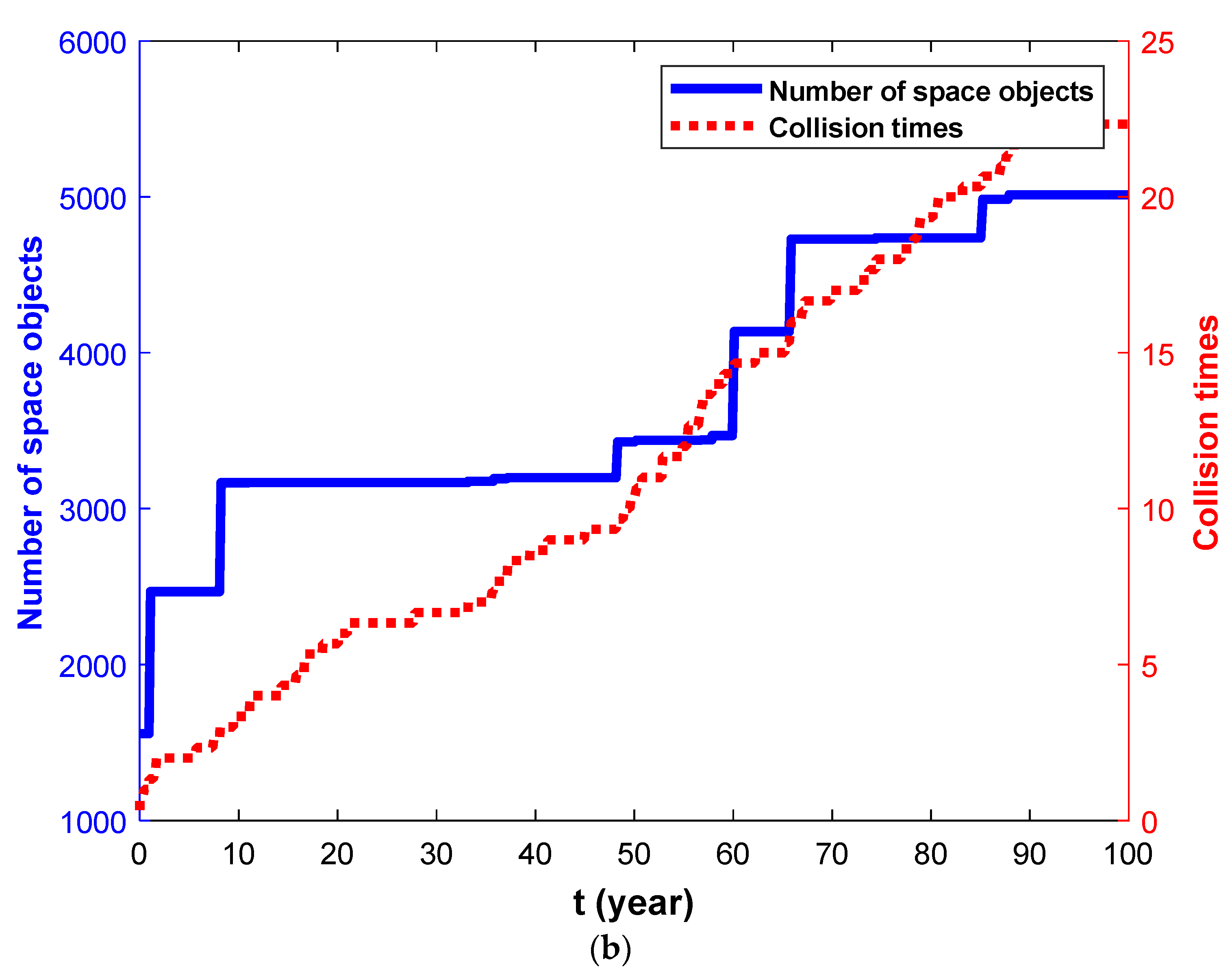
3.1.2. Scenario No. 2

In scenario No. 2, AMC-2 collided with space debris from the GEO band at 0:00 on 1 February 2022. The classical orbital elements of the space debris are shown in Table 3. The relative velocity was 802.6 m/s. The mass of the space debris was 330 kg. The spacecraft and the space debris disintegrated completely. The space environment 100 years after the collision was simulated.
The results of 20 simulation experiments under this scenario are shown in Figure 3. The abscissa represents the order of the simulation experiments. The left ordinate represents the total number of space objects with a characteristic size greater than 0.05 m in the GEO band after 100 years. The right ordinate represents the total number of collisions within 100 years in the simulation. In 100 years, an average of 234 collisions occurred, and the total number of GEO space objects after 100 years averaged 48,443. The standard deviation of the number of collisions was 5.3, and the standard deviation of the total number of space objects after 100 years was 2423.1.
The simulations with the largest and smallest number of space objects after 100 years in this scenario are shown as Figure 4. The red dotted lines represent the total number of collisions since the first collision at 0:00 on 1 February 2022, and the blue solid lines represent the number of space objects larger than 0.05 m in the GEO band.
Within 100 years after the first collision, 228 and 241 collisions occurred in the simulations depicted in Figure 4a,b, respectively. The amount of space debris produced by the initial collision was 1736, and the total number of GEO space objects increased from 3247 to 52,253 and 43,480, respectively.

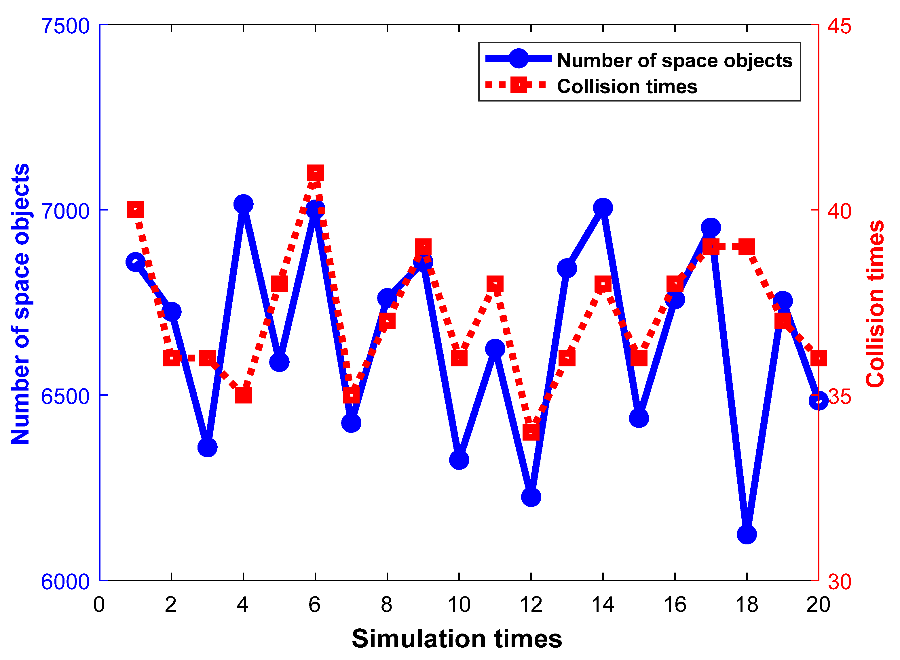
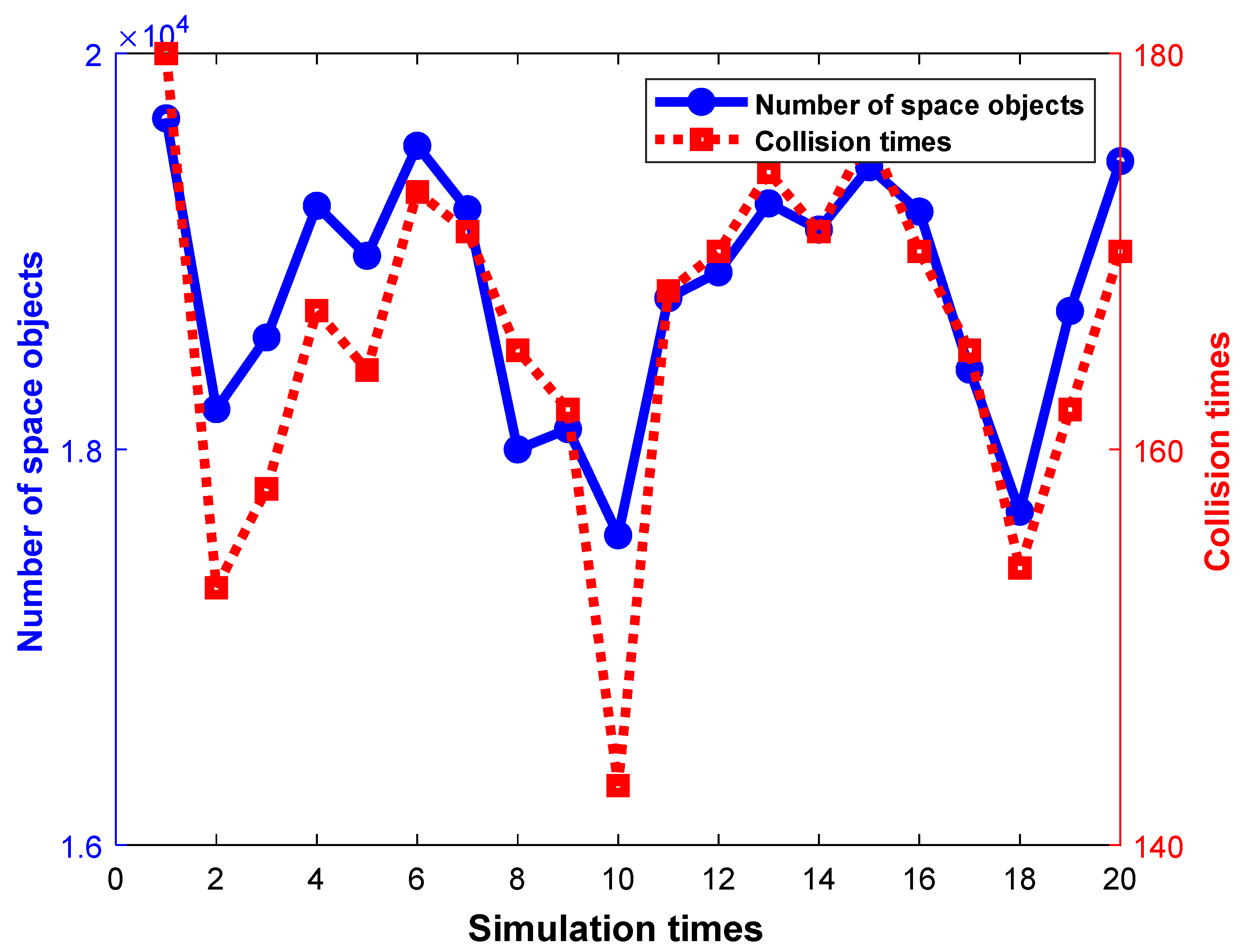
3.2. Incomplete Disintegration Simulation

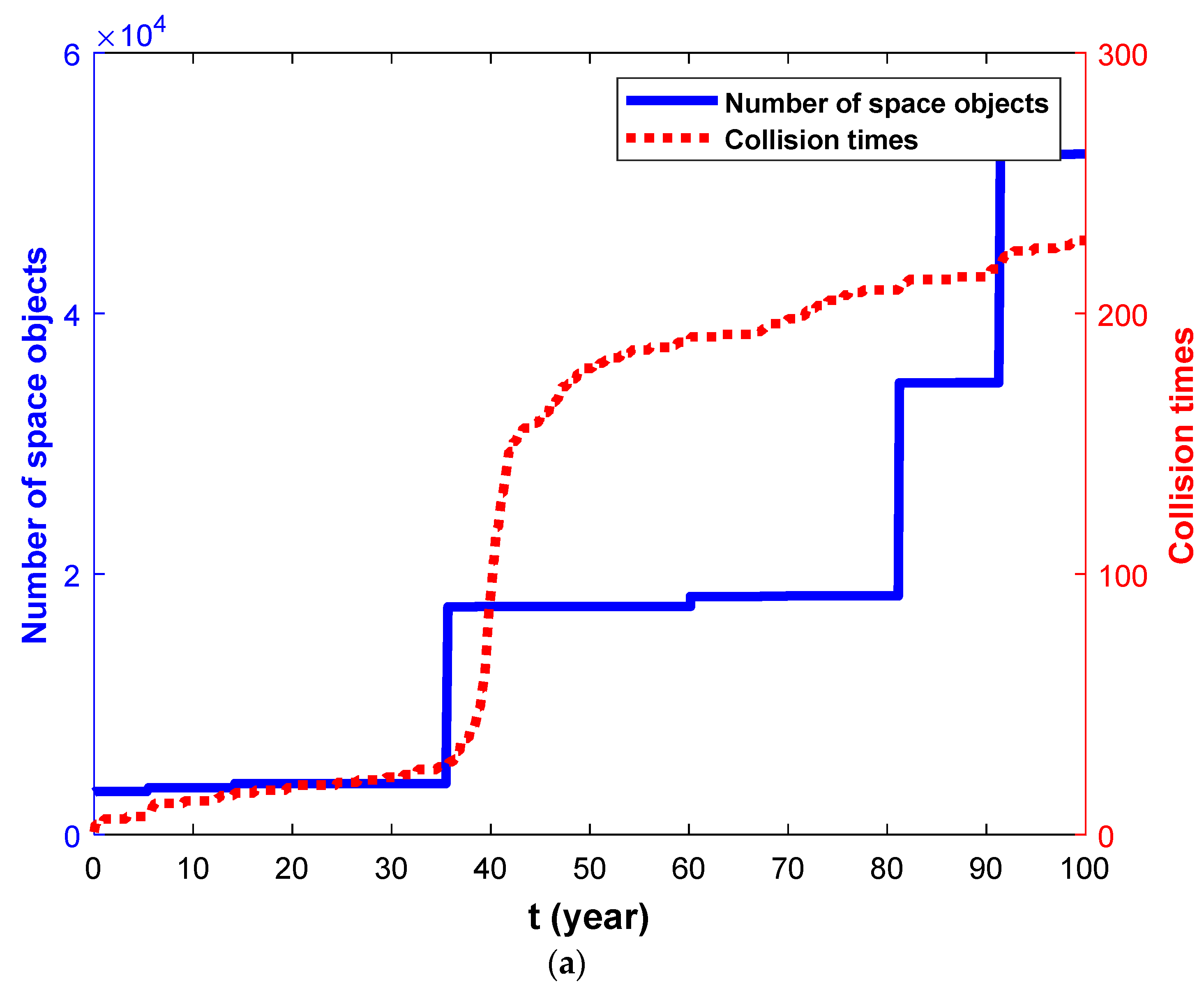
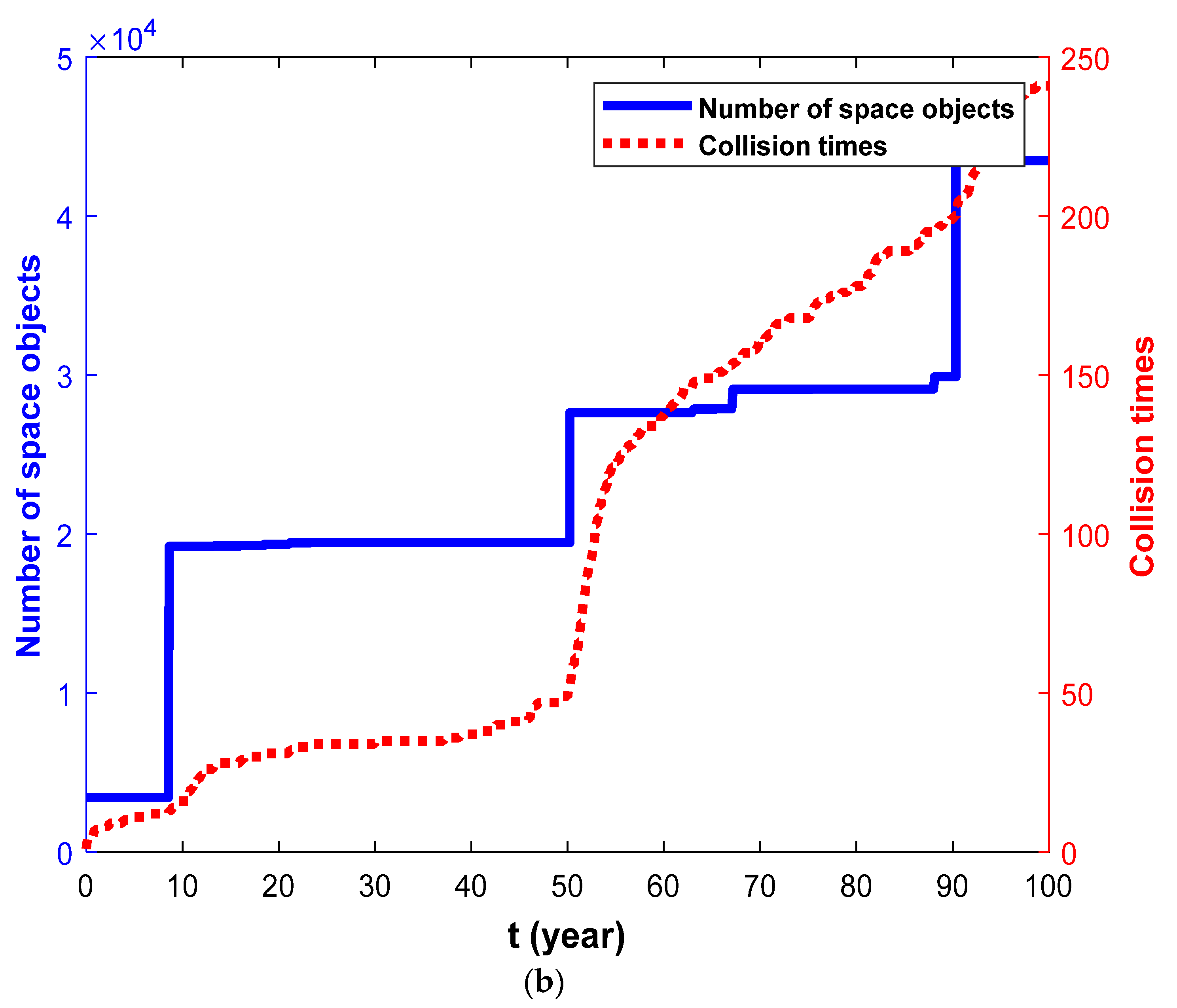
3.2.1. Scenario No. 3

In scenario No. 3, AMC-2 collided with space debris from the Molniya orbit at 0:00 on 1 February 2022. The classical orbital elements of the space debris are shown in Table 2. The relative velocity was 2980.6 m/s. The mass of the space debris was 8 kg. The spacecraft and the space debris disintegrated incompletely. The space environment 100 years after the collision was simulated.
The results of 20 simulation experiments under this scenario are shown in Figure 5. The abscissa represents the order of the simulation experiments. The left ordinate represents the total number of space objects with a characteristic size greater than 0.05 m in the GEO band after 100 years. The right ordinate represents the total number of collisions within 100 years in the simulation. In 100 years, an average of 37 collisions occurred, and the total number of GEO space objects after 100 years averaged 6656. The standard deviation of the number of collisions was 1.8, and the standard deviation of the total number of space objects after 100 years was 272.7.
The simulations with the largest and smallest numbers of space objects after 100 years in this scenario are shown as Figure 6. The red dotted lines represent the total number of collisions since the first collision at 0:00 on 1 February 2022, and the blue solid lines represent the number of space objects larger than 0.05 m in the GEO band.
Within 100 years after the first collision, 35 and 39 collisions occurred in the simulations depicted in Figure 6a,b, respectively. The amount of space debris produced by the initial collision was 142, and the total number of GEO space objects increased from 1653 to 7015 and 6124, respectively. Eight of the 74 collisions occurred between the newly disintegrated debris, and the remaining 66 collisions occurred between the original space objects.

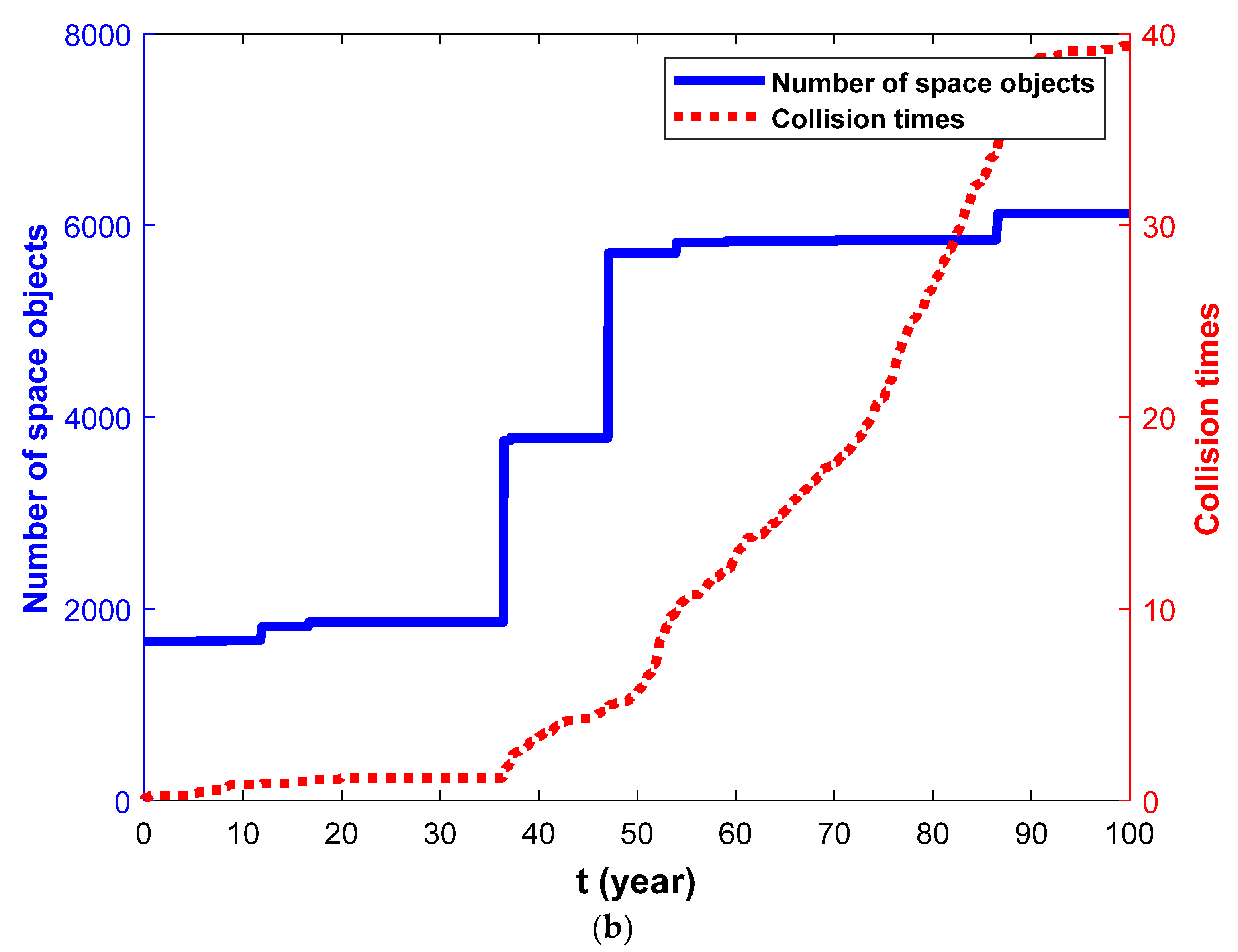
3.2.2. Scenario No. 4

In scenario No. 4, AMC-2 collided with space debris from the GEO band at 0:00 on 1 February 2022. The classical orbital elements of the space debris are shown in Table 3. The relative velocity was 802.6 m/s. The mass of the space debris was 8 kg. The spacecraft and the space debris disintegrated incompletely. The space environment 100 years after the collision was simulated.
The results of 20 simulation experiments under this scenario are shown in Figure 7. The abscissa represents the order of the simulation experiments. The left ordinate represents the total number of space objects with a characteristic size greater than 0.05 m in the GEO band after 100 years. The right ordinate represents the total number of collisions within 100 years in the simulation. In 100 years, an average of 20 collisions occurred, and the total number of GEO space objects after 100 years averaged 5039. The standard deviation of the number of collisions was 1.3, and the standard deviation of the total number of space objects after 100 years was 12.5.
The simulations with the largest and smallest numbers of space objects after 100 years in this scenario are shown as Figure 8. The red dotted lines represent the total number of collisions since the first collision at 0:00 on 1 February 2022, and the blue solid lines represent the number of space objects larger than 0.05 m in the GEO band.
Within 100 years after the first collision, 21 and 22 collisions occurred in the simulations depicted in Figure 8a,b, respectively. The amount of space debris produced by the initial collision was 45, and the total number of GEO space objects increased from 1556 to 5053 and 5014, respectively. Among the 43 collisions, 5 occurred between the newly disintegrated debris, 6 occurred between the new disintegrated debris and the original space objects, and the remaining 32 collisions occurred between the original space objects.
There was uncertainty about the occurrence of collisions in the simulations. For the 20 simulations in each scenario, although the results of each simulation were different, the numbers of newly generated space objects and the numbers of collisions in each simulation were close to each other. The simulation results of the “Grid” model for the future space environment were stable.

4. Conclusions

According to the orbital characteristics of the space objects in the GEO band, a long-term evolution model, the “Grid” model, was established. The “Grid” model was used to study the space environment in the GEO band after the collision between GEO spacecraft and space debris. The four types of scenarios were simulated many times, and the conclusions were as follows:
First, once space debris collided with the GEO spacecraft and both completely disintegrated, the number of space objects increased rapidly. Consequently, the probability of collision increased significantly. With the spread of space debris, the spatial distribution was relatively stable, and the probability of collision gradually decreased, but collisions continued to occur;
Second, the greater the mass of the space debris colliding with the GEO spacecraft was, the greater the relative velocity was, and the more serious the consequences were. The deterioration in the GEO environment caused by the two complete disintegration events was much greater than that of the two incomplete disintegration events.
Once the space debris and the massive spacecraft were completely disintegrated after collision, the number of space objects increased rapidly, the collision probability also increased sharply, and the collision cascading syndrome occurred. However, during the lifetime of the spacecraft, the probability of the initial collision between the spacecraft and space debris was small, especially for scenarios 1 and 2.
From the two scenarios of incomplete disintegration, even if there was no initial disintegration event, collision and disintegration events occurred in the long-term evolution of the GEO band, which led to an increase in the number of space objects. However, compared with the scenarios of initial complete disintegration, the collision probability was much lower, and the number of space objects grew much more slowly.

Author Contributions

Conceptualization, Z.L.; data curation, H.Z. and W.W.; formal analysis, H.Z. and W.W.; funding acquisition, Y.Z.; investigation, Z.L.; methodology, Z.L.; project administration, Z.L.; resources, Z.L. and Y.Z.; software, H.Z. and W.W.; validation, Z.L.; visualization, H.W. and Y.Z.; writing—original draft, H.Z. and H.W.; writing—review and editing, Z.L. All authors have read and agreed to the published version of the manuscript.

Funding

The work was supported by the National Outstanding Youth Fund, under Grant 2017-JCJQ-ZQ-005, and the National Natural Science Foundation of China, under Grant 61304228.

Conflicts of Interest

The authors declare no conflict of interest.

References

  1. Li, Y.; Li, Z.; Shen, H. Numerical Simulation of Satellite Collision Breakup in GEO. J. Aerosp. Shanghai 2011, 28, 47–72. [Google Scholar]
  2. Li, H. Geostationary Satellites Collocation; National Defense Industry Press: Beijing, China, 2010; pp. 34–46. [Google Scholar]
  3. Zhang, H.; Li, Z.; Wang, W.; Wang, H.; Zhang, Y. Trajectory Planning for Optical Satellite’s Continuous Surveillance of Geostationary Spacecraft. IEEE Access 2021, 9, 114282–114293. [Google Scholar] [CrossRef]
  4. Inter-Agency Space Debris Coordination Committee. IADC Space Debris Mitigation Guidelines; UN COPUOS 40th session; Inter-Agency Space Debris Coordination Committee: Vienna, Austria, 2002; revised 2007. [Google Scholar]
  5. Dongfang, W.; Baojun, P.; Weike, X.; Keke, P. GEO objects spatial density and collision probability in the Earth-centered Earth-fixed (ECEF) coordinate system. Acta Astronaut. 2016, 118, 218–223. [Google Scholar] [CrossRef]
  6. ESA Space Debris Office. ESA’s Annual Space Environment Report; Technical Report GEN-DB-LOG-00288-OPS-SD; European Space Operations Centre: Darmstadt, Germany, 2021. [Google Scholar]
  7. Murtaza, A.; Pirzada, S.; Xu, T. Orbital Debris Threat for Space Sustainability and Way Forward. IEEE Access 2020, 8, 61000–61019. [Google Scholar] [CrossRef]
  8. Sanny, R.; Bevilacqua, R. Spacecraft Collision Avoidance Using Aerodynamic Drag. J. Guid. Control. Dyn. 2020, 43, 567–573. [Google Scholar]
  9. Shan, M.; Shi, L. Comparison of Tethered Post-Capture System Models for Space Debris Removal. Aerospace 2022, 9, 33. [Google Scholar] [CrossRef]
  10. Zhang, Y.; An, F.; Liao, S.; Wu, C.; Liu, J.; Li, Y. Study on Numerical Simulation Methods for Hypervelocity Impact on Large-Scale Complex Spacecraft Structures. Aerospace 2022, 9, 12. [Google Scholar] [CrossRef]
  11. Hobbs, K.; Davis, J.; Wagner, L.; Feron, E. Formal Specification and Analysis of Spacecraft Collision Avoidance Run Time Assurance Requirements. In Proceedings of the 2021 IEEE Aerospace Conference (50100), Big Sky, MT, USA, 6–13 March 2021; pp. 1–16. [Google Scholar]
  12. Mote, M.; Hays, C.; Collins, A.; Feron, E.; Hobbs, K.L. Natural Motion-based Trajectories for Automatic Spacecraft Collision Avoidance During Proximity Operations. In Proceedings of the 2021 IEEE Aerospace Conference (50100), Big Sky, MT, USA, 6–13 March 2021; pp. 1–12. [Google Scholar]
  13. Xie, Z.; Chen, X.; Ren, Y.; Zhao, Y. Design and Analysis of Preload Control for Space Debris Impact Adhesion Capture Method. IEEE Access 2020, 8, 203845–203853. [Google Scholar] [CrossRef]
  14. Reynolds, R.; Eichler, P. A comparison of debris environment projections using the EVOLVE and CHAIN models. Adv. Space Res. 1995, 16, 27–135. [Google Scholar] [CrossRef]
  15. Krisko, P. Long-term orbital environment modeling using EVOLVE 4.0. In Proceedings of the 38th Aerospace Sciences Meeting & Exhibit, Reno, NV, USA, 10–13 January 2000. [Google Scholar]
  16. Liou, J.C.; Hall, D.T.; Krisko, P.H.; Opiela, J.N. Legend—A three-dimensional LEO-to-GEO debris evolutionary model. Adv. Space Res. 2004, 34, 981–986. [Google Scholar] [CrossRef]
  17. Martin, C.; Walker, R.; Klinkrad, H. The sensitivity of the ESA DELTA model. Adv. Space Res. 2004, 34, 969–974. [Google Scholar] [CrossRef]
  18. Lewis, H.; Swinerd, G.; Williams, N.; Gittins, G. Damage: A dedicated geo debris model framework. In Proceedings of the 3rd European Conference on Space Debris, ESA SP 473, Darmstadt, Germany, 19–21 March 2001. [Google Scholar]
  19. Martin, C.; Lewis, H.; Walker, R. Studying the MEO&GEO space debris environment with the Integrated Debris Evolution Suite (IDES) model. In Proceedings of the 3rd European Conference on Space Debris, Darmstadt, Germany, 19–21 March 2001. [Google Scholar]
  20. Rossi, A.; Anselmo, L.; Pardini, C.; Jehn, R.; Valsecchi, G.B. The new space debris mitigation (SDM 4.0) long term evolution code. In Proceedings of the Fifth European Conference on Space Debris, ESA/ESOC, Darmstadt, Germany, 30 March–2 April 2009. [Google Scholar]
  21. Dolado-Perez, J.C.; Di Costanzo, R.; Revelin, B. Introducing MEDEE—A new orbital debris evolutionary model. In Proceedings of the 6th European Conference on Space Debris, ESASP-723, Darmstadt, Germany, 22–25 April 2013. [Google Scholar]
  22. Radtke, J.; Stoll, E. Comparing long-term projections of the space debris environment to real world data-Looking back to 1990. Acta Astronaut. 2016, 127, 482–490. [Google Scholar] [CrossRef]
  23. Wang, R. Research on Space Debris Environment Model; Information Engineering University: Zhengzhou, China, 2010; pp. 87–96. [Google Scholar]
  24. Liou, J.; Kessler, D.; Matney, M.; Stansbery, G. A new approach to evaluate collision probabilities among asteroids, comets, and Kuiper Belt objects LPI 1828. In Proceedings of the Lunar and Planetary Institute Science Conference, League City, TX, USA, 17–21 March 2003. [Google Scholar]
  25. Liou, J. Collision activities in the future orbital debris environment. Adv. Space Res. 2006, 38, 2102–2106. [Google Scholar] [CrossRef]
  26. Bai, X. Research on Collision Probability in Space Objects Collision Detection; National University of Defense Technology: Changsha, China, 2008; pp. 45–53. [Google Scholar]
  27. Zhang, H.; Zhang, Z.; Chen, S. Evolution of newly generated debris from geostationary satellites’ collision. J. Comput. Meas. Control 2019, 27, 149–154. [Google Scholar]
  28. Zhang, H.; Zhang, Z.; Wu, S.; Wei, B. Short-term Dangers of Geostationary Satellites’ Collision Debris. J. Aerosp. Shanghai 2019, 36, 67–78. [Google Scholar]
  29. Zhang, H.; Zhang, Z.; Chen, S. Research of Space Environment’s Long-term Evolution Model. J. Comput. Meas. Control 2019, 27, 240–244, 249. [Google Scholar]
  30. Johnson, N. NASA’s new breakup model of evolve 4.0. Adv. Space Res. 2001, 28, 1377–1384. [Google Scholar] [CrossRef]
  31. Wang, D.; Tang, J.; Liu, L. Performance Evaluation of the Semi-analytical Method in the Long-term Prediction of the Earth Satellite at 100yr Scale. J. Acta Astron. 2017, 58, 3.1–3.26. [Google Scholar]
  32. Wang, D. Semi-Analytical Method and Its Performance Evaluation in the Long-Term Evolution of Earth Satellite Orbit; Nanjing University: Nanjing, China, 2016; pp. 50–53. [Google Scholar]
  33. Cimmino, N.; Isoletta, G.; Opromolla, R.; Fasano, G.; Basile, A.; Romano, A.; Peroni, M.; Panico, A.; Cecchini, A. Tuning of NASA Standard Breakup Model for Fragmentation Events Modelling. Aerospace 2021, 8, 185. [Google Scholar] [CrossRef]
  34. Space-Track. Available online: www.space-track.org (accessed on 1 February 2022).
Figure 1. Twenty simulation experiments of scenario 1.
Aerospace 09 00258 g001
Figure 2. Two simulations of the first scenario: (a) simulation with the largest number of space objects after 100 years; (b) simulation with the smallest number of space objects after 100 years.
Aerospace 09 00258 g002aAerospace 09 00258 g002b
Figure 3. Twenty simulation experiments of scenario 2.
Aerospace 09 00258 g003
Figure 4. Two simulations of the second scenario: (a) simulation with the largest number of space objects after 100 years; (b) simulation with the smallest number of space objects after 100 years.
Aerospace 09 00258 g004aAerospace 09 00258 g004b
Figure 5. Twenty simulation experiments of scenario 3.
Aerospace 09 00258 g005
Figure 6. Two simulations of the third scenario: (a) simulation with the largest number of space objects after 100 years; (b) simulation with the smallest number of space objects after 100 years.
Aerospace 09 00258 g006aAerospace 09 00258 g006b
Figure 7. Twenty simulation experiments of scenario 4.
Aerospace 09 00258 g007
Figure 8. Two simulations of the fourth scenario: (a) simulation with the largest number of space objects after 100 years; (b) Simulation with the smallest number of space objects after 100 years.
Aerospace 09 00258 g008aAerospace 09 00258 g008b
Table 1. Four types of simulations.
TypeDebris SourceMassCollision VelocityDisintegration
1Molniya orbit252980.6 m/scompletely
2GEO band330802.6 m/scompletely
3Molniya orbit82980.6 m/sincompletely
4GEO and8802.6 m/sincompletely
Table 2. Classical orbital elements of space debris from Molniya orbit.
ElementDataElementData
a/m26,556,000Ω/°156.639
e0.7456ω/°345.037
i/°63.40m/°244.247
Table 3. Classical orbital elements of space debris from GEO band.
ElementDataElementData
a/m26,556,000Ω/°336.639
e0.6778ω/°0
i/°63.40m/°0
Publisher’s Note: MDPI stays neutral with regard to jurisdictional claims in published maps and institutional affiliations.

