Article

Systematic Reliability-Based Multidisciplinary Optimization by Parallel Adaptive Importance Candidate Region

1
School of Civil Aviation, Northwestern Polytechnical University, Xi’an 710072, China
2
Yangtze River Delta Research Institute of NPU, Taicang 215400, China
3
School of Mechanical Engineering, Suzhou University of Science and Technology, Suzhou 215009, China
*
Author to whom correspondence should be addressed.
Aerospace 2022, 9(5), 240; https://doi.org/10.3390/aerospace9050240
Submission received: 26 February 2022 / Revised: 6 April 2022 / Accepted: 11 April 2022 / Published: 26 April 2022
(This article belongs to the Special Issue Multidisciplinary Multiobjective Design Optimization)

Abstract

:
Reliability-based design optimization (RBDO) has become a prevalent design for aeronautical and aerospace engineering. The main problem is that it is impractical in complex cases with multi-failure regions, especially in multi-objective optimization. The active learning method can obtain an adaptive size of samples to get a relatively acceptable accuracy. The problem of RBDO using the traditional active learning Kriging (ALK) method is that the design space is generally still and only one training point is selected, which is not reasonable based on the concept of importance sampling and parallel calculation. As a consequence, the accuracy improvement is limited. In this paper, we investigate the method of obtaining an optimal size of design and reliability to assess space in parallel, simultaneously. A strategy of parallel adaptive candidate (PAIC) region with ALK is proposed and a sequential optimization and reliability assessment (SORA) method is modified to efficiently improve the accuracy. Importance sampling is used as a demonstration for the modified SORA with more accuracy. The method is then verified using mathematical cases and a scooping system of an amphibious aircraft.

1. Introduction

Traditional reliability-based multidisciplinary optimization design (RBMDO) requires a large number of limit state function (LSF) calls or objective function (OBF) calls, which is time-consuming for the design of industrial products [1]. Meanwhile, the use of surrogate models, such as response surface, Kriging, neutral networks model and so on, can avoid directly calling the real LSFs and OBFs to increase the efficiency [2]. Besides, the accuracy of surrogate models can be improved furtherly by the process of sampling. The typical sampling method for the RBDO surrogate model generates all the samples at once, such as Monte Carlo, Orthogonal and Latin hypercube sampling [3]. Efforts have been made to minimize the samples of function evaluations and the active learning Kriging (ALK) method can increase the accuracy of the interest region by continuously and adaptively adding the training points, which has recently attracted interest for its better performance in solving complex problems (e.g., non-linear structures), with an acceptable computational cost and accuracy [4]. Based on the efficient global optimization (EGO), some have focused on developing the learning algorithm, or learning function (LF), to select new training points to increase accuracy [5,6,7].
For optimization with the Kriging model, LF has been improved and adapted into different types by different importance sampling purposes, including expected improvement (EI) [8], U-function [2], expected feasibility function (EFF) [9], expected risk function (ERF) [10], importance learning method (IL) [11], etc., and is then adopted in the RBDO problem. Further, some research applied them in combinations. Song et al. used the Bayesian probabilistic integration for data-driven and active learning of sensitivity indices and proved its efficiency with an original importance sampling method [12]. Zhang et al. proposed a novel LF, called reliability-based expected improvement function (REIF), for structural reliability problems [13]. Considering the distance from the real optimum and importance of reliability region, we have also proposed an expected improvement exponent (EIE) for optimization and expected risk function with importance (ERFI) for reliability [14].
The concept of importance sampling can also be used to increase the accuracy of reliability assessment with the efficient global reliability assessment (EGRA) [15]. Zhang et al. combined the low-discrepancy samples and adaptively truncated sampling regions to initiate efficient active learning iterations [13]. Wen et al. proposed an adaptive sampling region method, ISKRA, to avoid selecting the additional points where the probability density is low [16]. Yang developed a strategy to determine the minimal or optimal size of candidate points to handle the system reliability analysis, which focused on the problems in parallel computation [5]. They proposed a truncated candidate region Tk approach to approximate the kth adaptive sample region by deleting sample points from the adaptive insignificant region (AIR) T ˜ , which is determined by the average and deviation value of current predictive LSF. Yun et al. proposed an adaptive subdomain sampling method, which is determined by distance index PA and estimation failure probability Pf [17]. They gave a method for estimating the probability of the possible domain of uncertain variables that affect the failure probability, then, the possible domain of the uncertain distribution region is flexibly obtained. However, a method should include the capacity of parallel computing for systematic reliability problems. Influence function (IF) is introduced for parallel computing for optimization [18] and it could be modified for systematic reliability analysis. Wen et al. applied K-means for parallel computing in systematic reliability analysis [16]. These studies showed it would be of good performance if we combined IF and AIC, producing the PAIC method.
Recent works also focused on the strategy of RBDO’s solving loop structure, such as traditional double loop [19], single loop [20], subset simulation-based reliability analysis (SSRA) [21], multilevel nested system [22], and sequential optimization and reliability assessment (SORA) strategy [22,23]. We also presented a sequential reliability assessment and optimization (SRAO) strategy to simplify this computational structure [24]. Some impressive attempts have been made combined with simplifying the solving loop structures and the use of the active learning surrogate model.
In this paper, we propose an ALK method to update the adaptive importance candidate (AIC) region for RBDO problems. Combining with the LF method, the AIC region can fully use the information obtained from the irritated Kriging model and continually update the pre-selected sample regions according to this information. The AIC can be moved and shrunk with the optimization continuing, so that a simple sampling method can be applied to require a relatively high accuracy. With the modified SORA method, this paper tries to give a relatively simple method for RBDO. Then, some mathematical problems are verified and every case is tested several times, in order to demonstrate the stability.

2. Proposed Methods

2.1. Kriging Model

Kriging interpolation method is flexible and suitable for the approximation of many cases, because a wider range of correlation functions is presented for building the metamodel. Here, a series of response functions is assumed Y = [Y(x1), Y(x2),…, Y(xn)]T, where n is the sample size. Then, the predictive value of target function Y ^ ( x ) that is required to predict is:
Y ^ ( x ) = i = 1 p β i f i ( x ) + z ( x ) = f ( x ) T β + z ( x )
where z(x) is the random item, f(x) = [f1(x), f2(x), …, fp(x)]T is the regression polynomial basis function vector, p is the size of the regression polynomial. β = [β1, β2, …, βp]T is the regression coefficients vector. The covariance for w and x can be respectively described as
cov ( z ( w ) , z ( x ) ) = σ 2 R ( θ , w , x )
where R is correlation function and θ = [θ1, θ2, …, θn]T are correlation parameters. Because the Gaussian correlation function is widely used when the function is smooth or continuously differentiable, R(θ, w, x) is set as Gaussian form and can be written as
R ( θ , w , x ) = k n R k ( θ k , w k x k ) = exp ( k = 1 n θ k | w k x k | 2 )
The process variance σ and regression coefficients β can be written by the least square regression
β = ( F T R 1 F ) 1 F T R 1 Y
σ 2 = 1 k ( Y F β ) T R 1 ( Y F β )
where F is a matrix with Fij = fj(xi), i = 1, 2, …, k, j = 1, 2, …, m. Then, we can predict the value of target function using the following formulas
Y ^ ( x 0 ) = f ( x 0 ) T β + r 0 T R 1 ( Y F β )
σ ^ g ^ 2 = σ ^ 2 ( 1 + u T ( F T R 1 F ) 1 u r 0 T R 1 r 0 )
u = F T R 1 r 0 f ( x 0 )
where r0 is the correlation vector between x and each training point.

2.2. Learning Functions in Active Learning Method

Learning function (LF) is the key technique in ALK, can give a mathematical method to judge which sample has the most value to train the ALK model. They have been studied and developed to increase the accuracy of ALK for different purposes.
Expected improvement (EI) function is widely used in global optimization problem [8], the kth EI is
E I k = ( g min g ^ k ( x ) ) ϕ ( g min g ^ k ( x ) σ ^ g ^ k ( x ) ) + σ ^ g ^ k ( x ) ψ ( g min g ^ k ( x ) σ ^ g ^ k ( x ) )
where g min = min [ g ^ ( x ) ] , ϕ ( ) and ψ ( ) are the standard normal cumulative function and the standard normal probability density function, respectively. Thus, samples can gradually focus on the region near the optimum gmin.
Expected risk function (ERF) can improve the accuracy of LSF predicting by learning the training point with the largest risk that its sign is wrongly predicted [5]
E R F k = s i g n ( g ^ ( k ) ( x ) ) g ^ ( k ) ( x ) ϕ ( s g n ( g ^ ( k ) ( x ) ) g ^ ( k ) ( x ) σ ^ g ^ ( k ) ( x ) ) + σ ^ g ^ ( k ) ( x ) ψ g ^ ( k ) ( x ) σ ^ g ^ ( k ) ( x )
The larger the value of ERF means a higher possibility of predicting wrongly from positive to negative or from negative to positive.
Reference [14] proposed a new acquisition function, named EI with exponent acceleration (EIE), to avoid selecting the boundary points even when they are far from the optimum point. In this paper, we improve EIE acquisition function for a more stable performance
E I E = ( g min g ^ ( k ) ( x ) ) ϕ ( g min g ^ ( k ) ( x ) σ ^ g ^ ( k ) ( x ) ) E X P ( x min x k η ) + σ ^ g ^ ( k ) ( x ) ψ ( g min g ^ ( k ) ( x ) σ ^ g ^ ( k ) ( x ) )
where η = max ( x min x 1 k , x min x 2 k , , x min x n k ) , xmin is minimal point, n is the number of elements in the total candidates, which is often larger than the number of original sample points. Its convergence condition is δ max = max [ E I E ( f ^ ( x ) ) ] ε . However, this leads to a higher probability to fall into a local optimum.
Thus, an improvement exponent distance (EID) function that adds a new item representing the error of selecting points too far from the current predicted optimum point:
{ E I D ( 1 ) = E I E ( f ^ ( x ) ) E I D ( p ) ( f ^ ( x ) ) = E I ( p ) ( f ^ ( x ) ) + E I D ( p 1 ) ( f ^ ( x ) ) E X P ( x min x k η )
where p is a positive integer indicating the number of iterations. Convergence condition is
δ max = max ( E I D ( p ) ) max ( E I D ( p 1 ) ) ε
If we want to obtain a global optimum with the error of ε, N is required above 102−log(ε). For example, ε = 0.01 requires 104 samples.

2.3. Coupling Methods for MDO

A typical RBMDO includes the analyses of several different disciplines, which are often coupled with each other. The mathematical model of RBMDO can be described as
f i n d d ,   μ x ; min f ( d ,   μ x , μ P ) s . t . p r o b ( G i ( d , X , P ) 0 ) R i , i = 1 , 2 , , n g j ( d ,   μ x , μ P ) 0 , j = 1 , 2 , , n h ( d ,   μ x ) = 0 ( i , j ) { 1 , , N } , i j , y i j = c j i ( d , y * j ) d [ d L , d U ] ,   X ~ N ( μ x , σ x )
where d is deterministic design vector, μ x is averaged uncertain design vector, μ P is the uncertain parameters, G i ( d , X , P ) 0 and g j ( d ,   μ x , μ P ) are reliability and deterministic constraints, respectively, i and j are the number of uncertain and deterministic constraints.   f ( d ,   μ x , μ P ) is objectives function (OBF), and h is the constraint vector of inter-disciplinary consistency, which can be stated as the maximal difference between yij and yji, where
{ y i j = c j i ( d , y * j ) y j i = c j i ( d , y * j )
The multidisciplinary feasible method (MDF) sequentially analyses the different disciplines and connects them by solving the interdisciplinary consistency (shown in Figure 1). Thus, the h can be set as one of constraints when conducting the RBMDO.

2.4. Parallel Adaptive Importance Candidate Region (PAIC)

However, general methods of the ALK model need to build a relatively large enough size of initial candidate training points, which is sampled at the first time and keeps constant through the whole modelling process. Problems occur, where the accuracy will reach a limit threshold value if real optimum is not covered by the initial samples.
In system reliability assessment, importance sampling (IS) is widely used to reduce the number of Monte Carlo simulations. The core of IS is to adjust the sampling center to the failure region, called importance sampling density (ISD). Then, the failure probability is
P f ( x ) = + + I f ( x ) f ( x ) h ( x ) h ( x ) d x = E [ I f ( x ) f ( x ) h ( x ) ]
where hX (x1, x1, …, xn) is the density function (PDF) of a new distribution. If(x) is the failure indicator function for g(x), which can be expressed as
I f ( x ) = { 1 , g min ( x ) 0 0 , g min ( x ) > 0
Then Pf can be estimated by IS by
P ^ f = 1 N i = 1 N [ I f ( x i ) f ( x i ) h ( x i ) ]
Var [ P ^ f ] = 1 N 1 { 1 N i = 1 N [ I f ( x i ) f ( x i ) 2 h ( x i ) 2 ] ( P ^ f ) 2 }
Generally, main task of IS is to construct sampling function h(x) based on the design point x*, which is called most probable point (MPP) in reliability assessment or current optimal point (COP) in optimization. Here, normal hX(x) is built for AIR as
h X ( x ) = 1 2 π σ * exp ( ( 1 x * ) 2 2 π σ * 2 )
where x = [ x 1 , x 2 , , x n ] T is the probable sample point, n is the dimension of variables. The sample points in IS set are remarked as x I S ( x * , σ * ) . The density center of sampling function h(x) is therefore equal to the x*. Based on this, we proposed two different importance learning methods for sequential optimization and reliability assessment (SORA), respectively. Obtaining x* for reliability assessment, or xMPP, is defined as an optimal problem
f i n d x M P P min U g i ( x )   s . t . U = β
where the index β relates to reliability requirement R, this method is therefore called reliability index method. It requires one to transfer the random abnormal or non-standard normal parameters into the mutually independent standard normal space (Ux, Up) by Rosenblatt or Nataf method [25]. Then, the probability can be calculated by
Pr ( g i ( x ) 0 ) = Φ ( β )
Here Φ is the standard normal distribution function. Add the points set
x a d d = { x a d d | | g ( x ) | ε I S I S ( x * , σ * ) }
to update the ALK model, and ε I S is user-designed error parameter which is related to the accuracy. The value of σ * is equal to index β. Then we can obtain the reliability by Equation (20). Parallel computing method IF is applied when multilocal optimal points or multi-failure regions exist, which can be written as
I F ( x , x u ) = 1 exp ( k = 1 d θ k | x k ( i ) x k u | P k )
where x k u is the update point, d is the number of test points, θk and Pk can be set as required, generally, θk = 1 and Pk = 2 [18]. The x k u is therefore degraded to select the second parallel training point. The number of parallel samples np in one iteration can be also adaptive based on the convergence criterion ε. Here, np can be simply set as
n p ( i + 1 ) = { i + 1 , ε p ( i ) ε / ζ [ ζ n p ( i ) ] , ε p ( i ) < ε / ζ w h e r e ε p ( i ) = 1 | max ( L F ( x ) I F ( x , x u ) ) ε | ( max ( L F ( x ) I F ( x , x u ) ) )
ζ ( 0 , 1 ] are the adaptive shrunk coefficients related to required accuracy ε , generally set ζ = 0.6 ~ 0.8 .
For optimization, the point with the largest value of learning function LF(x), such as EI or EIE, is set as the update (training) point x*,
x * = arg max i = 1 n [ LF ( x ) IF ( x , x u ) ]
We can then define the probability when the real optimal point locates in the current PAIC regions as
P ( x ) = β β f ( x ) d x > P P A I C
Here, the estimated value f(x)~N(μf(x), σ2f(x)) by ALK, where   μ f ( x ) = f ^ ( x ) and   σ f ( x ) = s f ( x ) . We can then obtain ith PAIC region with a center of x ^ * P A I C and a radii-vector s * P A I C
x ^ * P A I C = arg max i = 1 n [ L F ( x ) I F ( x , x u ) ] s * P A I C = ϕ ( 1 ) ( P P A I C N ) σ ^ f ^ ( i ) σ ^ f ^ ( 0 )
where, PPAICN is the transferred probability in standard normal space based on Equation (28). By solving estimated average value x ^ * and estimated standard variance s ^ * of design point, PAIC regions can therefore be updated at each iteration. Different from the adaptive regions proposed by other studies [5,16], the area changes in PAIC regions are treated as a probability event.
For reliability, the point with the largest value of learning function, such as ERF (Equation (10)), is set as the update point xu. If we treat the PAIC region as a high-dimensional ellipsoid, then the s * P A I C can be seen as its minimal diameter. If the predicted optimal value of the objective functions stands still, the index should be further shrunk to help convergence. In Equation (28), the item of σ ^ f ^ ( i ) / σ ^ f ^ ( 0 ) relating to the accuracy of ALK, will decrease with the continuous learning from the additional training points and the areas of PAIC regions will shrink and the accuracy of the optimal point will increase. Therefore, we can use the term σ ^ f ^ ( i ) / σ ^ f ^ ( 0 ) < ε as a stopping criterion. Steps are as follows:
Step (1)
Build initial ALK for optimization. Use initial smaller size of samples and build ALK for optimization (Optmodeli) with additional p samples to find estimated optimum d(0) by updating LF, where i is the number of OBFs.
Step (2)
Find MPPs by ALK. Compute reliability index β by transferring the random parameters to the standard normal distribution. Generate a point set in size j within β, and build ALK for reliability (Relmodelj). The updating by learning function of Relmodelj is used for searching the minimum LSFs of points Gj(xβ). It should be noted that the rough MPP candidate points xβ with lower accuracy are based on IS.
Step (3)
Update the initial design by reliability requirements. Add new points xadd for IS(x*, σ*) in parallel to train the Relmodelj with higher accuracy based on formular Equation (24) (j is the number of OBFs and LSFs). The accuracy is related to ε I S .
Step (4)
Estimated optimum searching under estimated probabilistic constraints. Set initial convergence ε(0) is 1000. Search the optimum by the ALK optimization. The MPP search is based on existing Relmodelj without calling LSF.
Step (5)
Judge the real reliability. Search MPP at the estimated optimum based on step (2) and use IS method to calculate the reliability. However, if Gj(xβ) > 0, ALK is unnecessary; otherwise, LF method is used to train points to update the Relmodelj.
Step (6)
Use IS to calculate the reliability requirements. If Gj(xβ) < 0, calculate the reliability with IS by ALK. If Gj(xβ) is still below zero, return to step (4), and if all G(xβ) > 0, reliability meets the requirement and optimization convergence is also achieved, then, dopt = d(k) (Equation (29)) and end.
  d ( k + 1 ) = d ( k ) d s | G min ( x ^ M P P ( k ) ) | G ( d ( k ) ) G min ( x ^ M P P ( k ) ) ( x ^ M P T P ( k ) d ( k ) )

3. Analysis and Results

3.1. Optimization of Double-Peak Function

This example has two peaks but only one global optimum, from reference [26] (Figure 2a), where z1, z2 and z3 are three coupled disciplines, and h(z1, z2, z3) is the inter-disciplinary consistency, as shown in Equation (30).
find   X = [ X 1 , X 2 ] T min y ( X ) = ( z 1 + z 2 + z 3 ) s . t . z 1 = 60 / [ 1 + ( X 1 + 1 ) 2 + ( X 2 3 ) 2 ] ; z 2 = 20 / [ 1 + ( X 1 1 ) 2 + ( X 2 3 ) 2 ] ; z 3 = 30 / [ 1 + X 1 2 + ( X 2 + 4 ) 2 ] ; X i [ 8 , 8 ] , i = 1 , 2
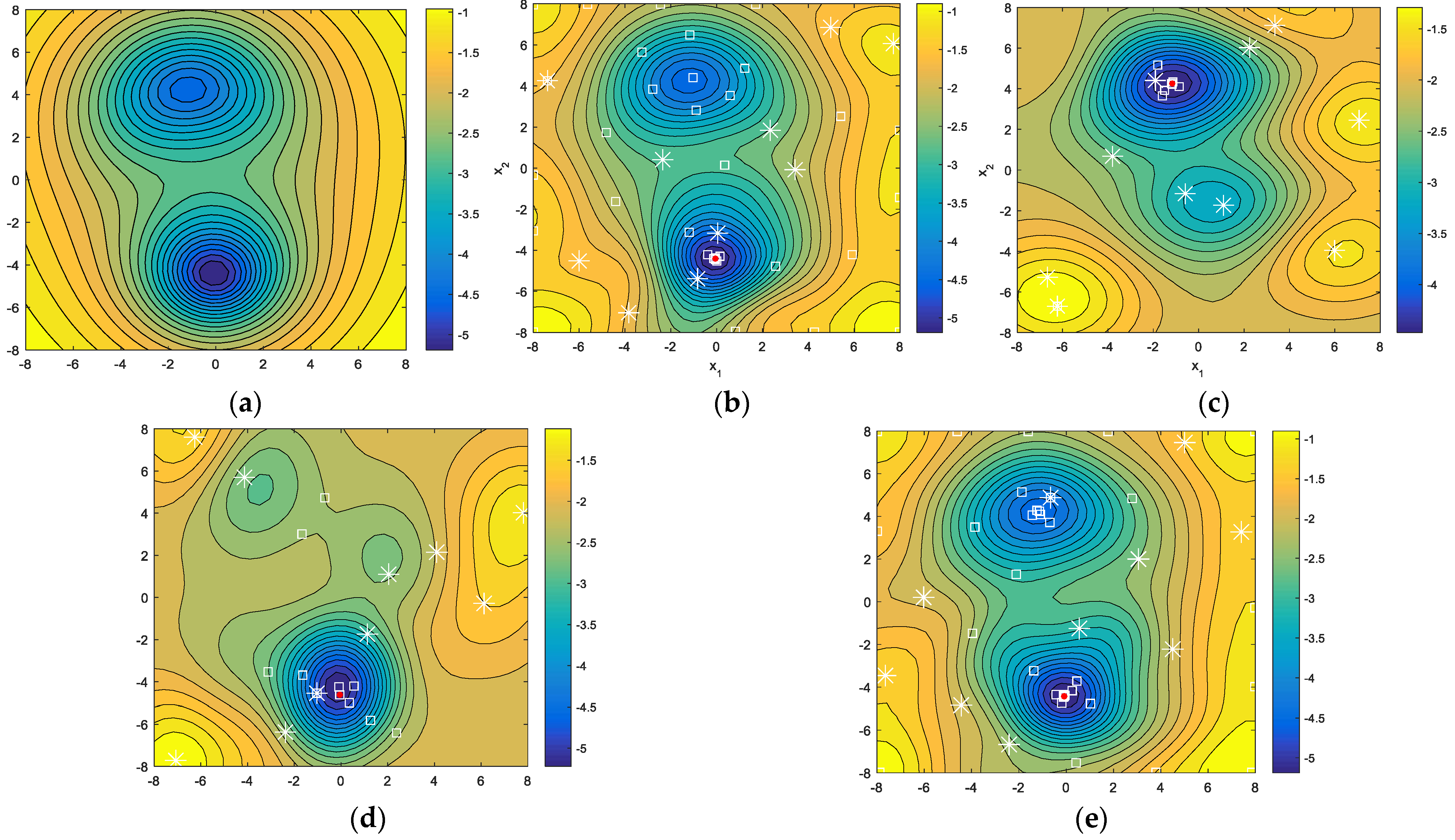
The results are shown in Figure 2. EID could find the global optimum (Figure 2b), while EIE would have a large probability to find the local optimum (Figure 2c). EIE accelerates the convergence but is easily trapped in the error local result. AIC will find the global optimum by the least training points (Figure 2d). Besides, PAIC can also find the local optimum, as shown in Figure 2e. The IF can degrade the global learning potential points and search the extra important region where the local candidate points may be located. This demonstrates that AIC has a relatively high efficiency and PAIC has an ability to search the local optimum, as well as the global optimum.

3.2. Multi-Failure Systems with Four Branches

Systemic reliability analysis generally includes several limit states functions. This example includes four branches, which is a systemic reliability problem, from reference [16], and is presented here to show its performance on the reliability assessment, shown in Equation (31). ΜX = (1,1) and β = 1.8 are selected as the base point and reliability index, respectively and the limit state function (LSF) is
g ( X ) = min { 3 + 0.1 ( X 1 X 2 ) 2 ( X 1 + X 2 ) / 2 3 + 0.1 ( X 1 X 2 ) 2 + ( X 1 + X 2 ) / 2 ( X 1 X 2 ) + 8 / 2 ( X 2 X 1 ) + 8 / 2 }
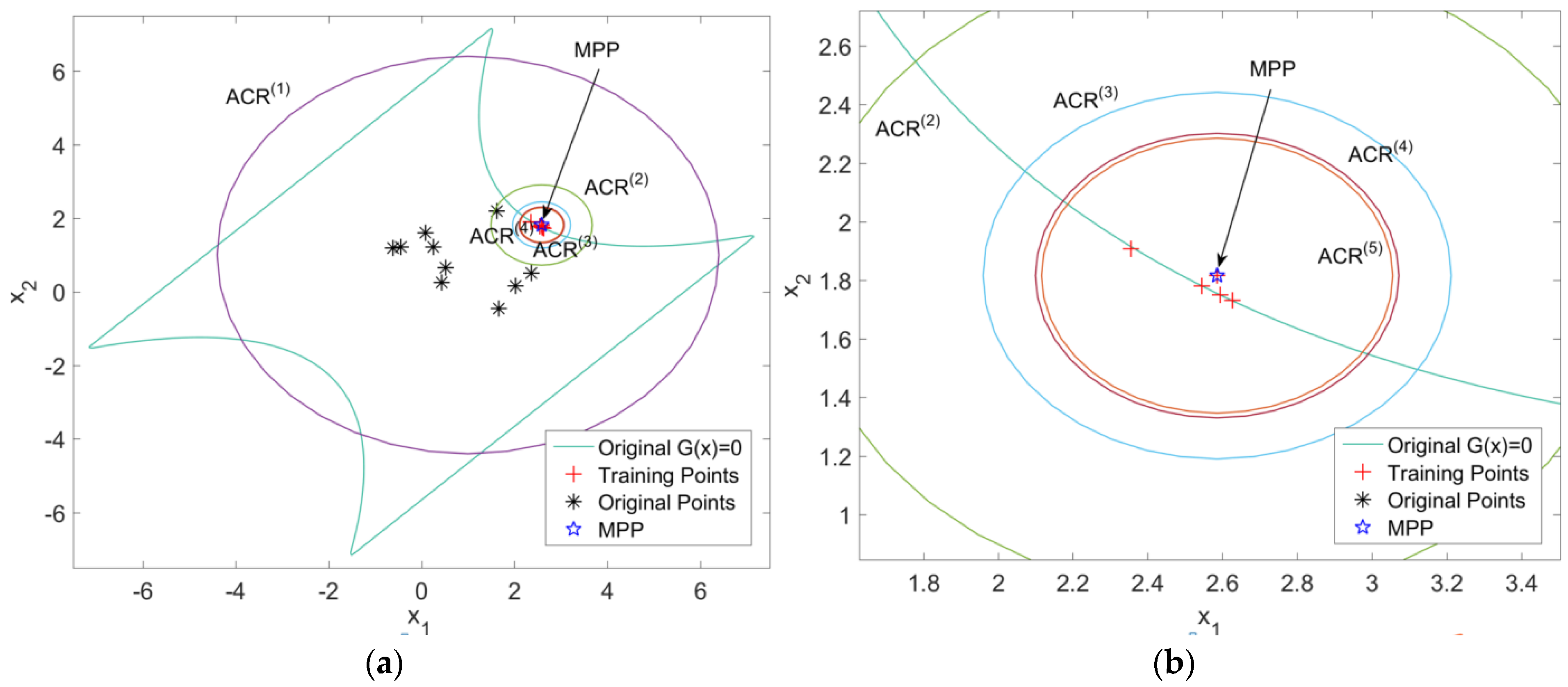
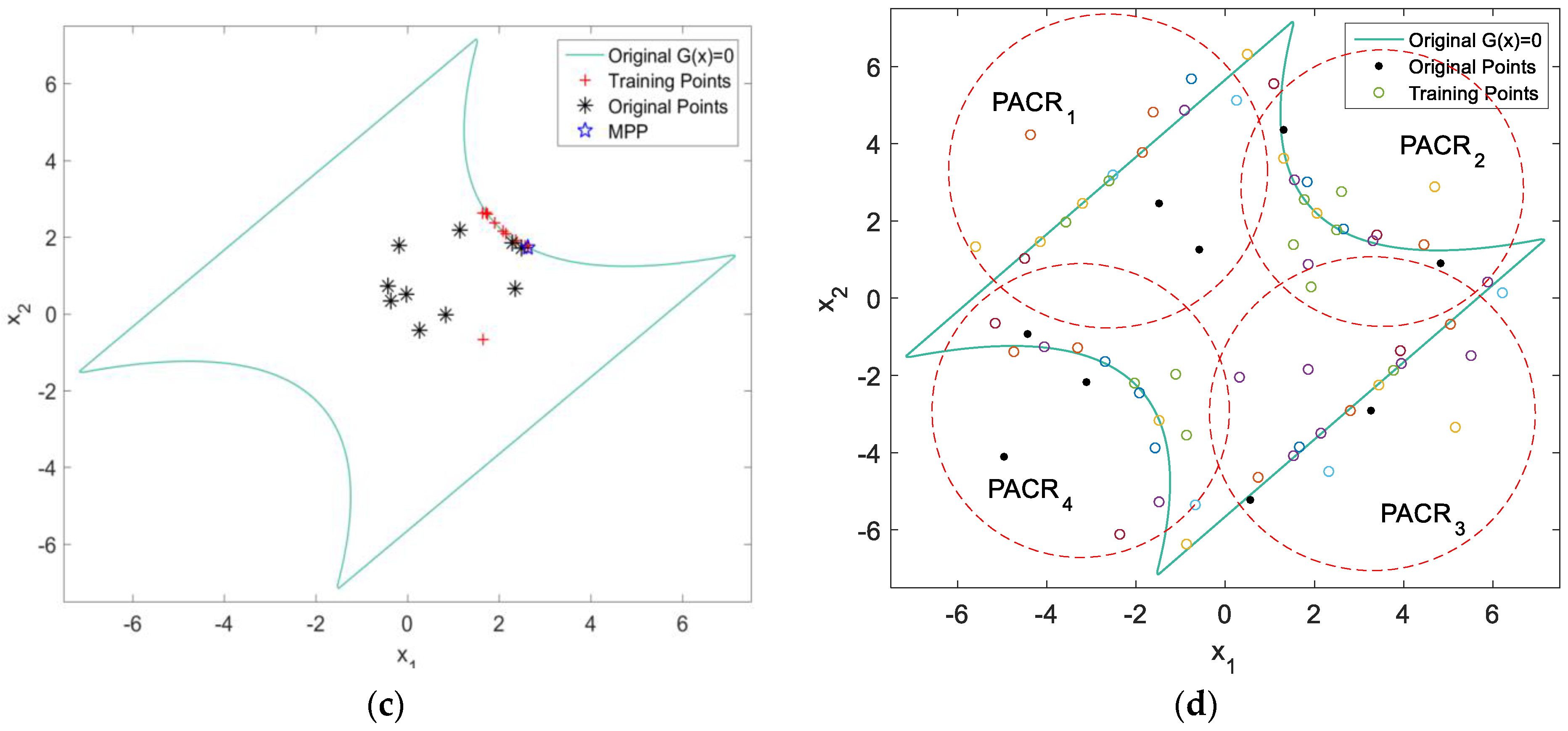
The ALK-AIC method can rapidly find out the MPP for the further RBDO, shown in Figure 3. The learning function is ERF. It can be observed that the space of IS continuously shrunk and the sampling points become fewer and fewer (Figure 3a). The AIC was small enough to get the MPP (Figure 3b). Only 5 additional points are selected by the AIC method, while 13 points are learned without the AIC method, shown in Figure 3a,c. It can be easily found that the MMP is successfully obtained by AIC techniques. Compared with real optimization from searching MPP, the accuracy of AIC is 30% higher than that of no-ACI method. The advantages of IS can be easily observed.
The results of PAIC regions (ε = 10−7) are shown in Figure 3d, where the same color of training points means that they are trained together in the same learning iteration. The number of learning iterations averaged 11.60 in 100 repetitions. The average number of the adaptive parallel number is 5.546.
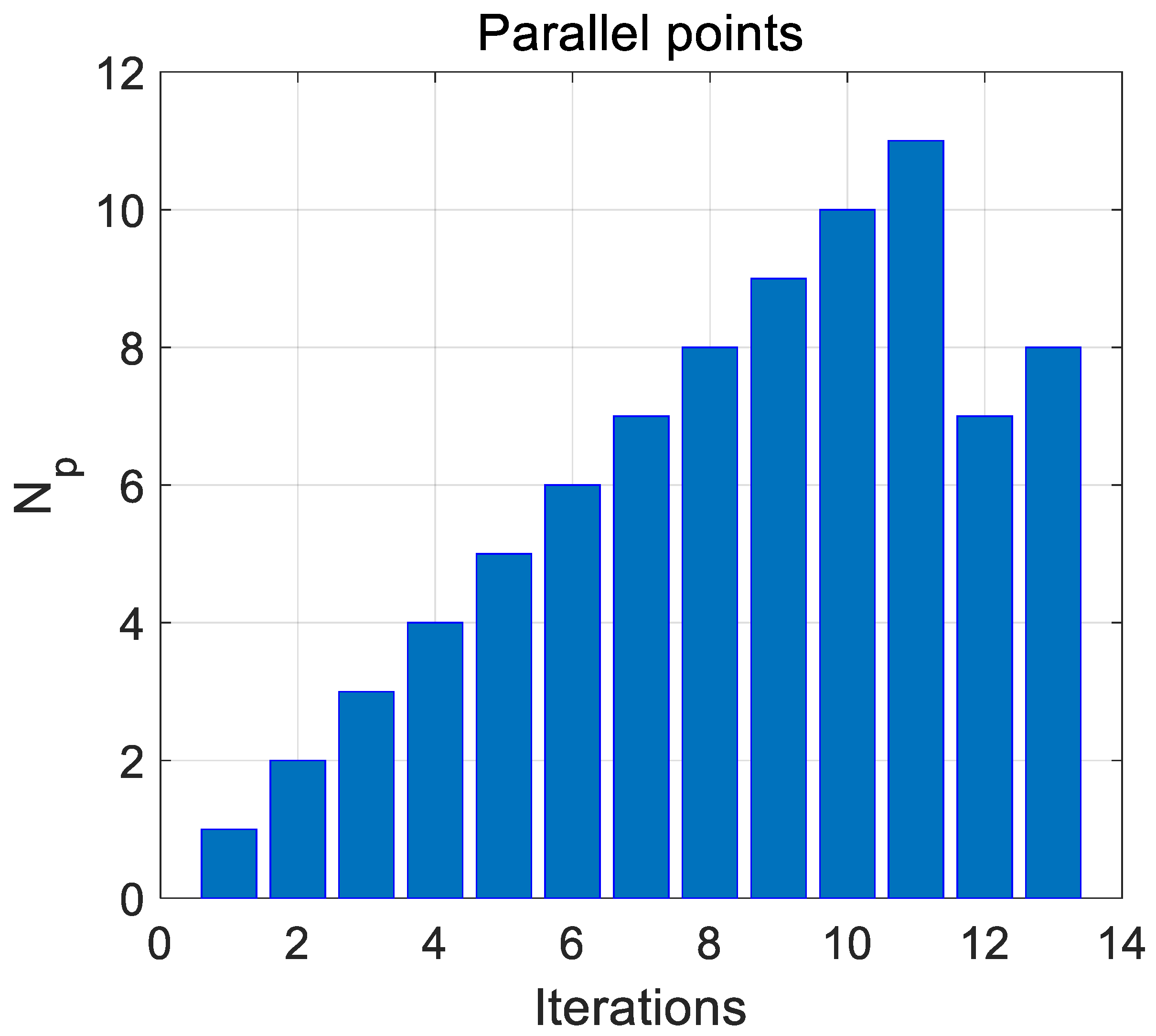
In order to test the performance of the PAIC method in small failure reliability assessment, we set X i ~ N ( 0 , 1 ) , i = 1 , 2 and all the tests were repeated 50 times. Initial samples for all the Kriging models in Table 1 are 10. K-MCS uses Kriging directly to build the surrogate model and additional training points would be learned if the required accuracy (ε = 10−7) is not achieved. We used MCS and IS to obtain the failure probability. The result from MCS with 1.0 × 10⁹ simulations is treated as the comparison standard, i.e., Pf = 1.218 × 10⁻⁵. Therefore, MCS requires at least 1.0 × 10⁷, which is set as the number of other methods by ALK-MC. Compared with ISKRA, the number of Np is also dynamic, related to the distance to required accuracy, and here, ζ = 0.8 in Equation (23). The dynamic np in each iteration is shown in Figure 4. We can easily find that PAIC uses the least number of LSF calling and iterations.

3.3. RBMDO with Three Modes in Failure

An RBMDO example with the coupling of three failure modes, which is a type of systemic reliability assessment, is presented here, from reference [24], to show the performance of the PAIC technique, shown in Equation (32).
find   μ X = [ μ X 1 , μ X 2 ] T min y ( μ X ) = 1 2 sin ( μ X 1 2 ) + sin ( 3 μ X 2 2 ) s . t . p r o b [ ( g i ( X ) ) 0 ] 0.999 , i = 1 , 3 p r o b [ ( g 2 ( X ) ) 0 ] 0.999 μ X i [ 0 , 10 ] where   g 1 ( X ) = x 1 2 x 2 20 1 + g 3 ( X ) 80 , g 2 ( X ) = ( x 1 + x 2 5 ) 2 30 + ( x 1 x 2 12 ) 2 120 2 + g 1 ( X ) 20 , g 3 ( X ) = 80 x 1 2 + 8 x 2 + 5 0.5 + g 2 ( X ) , h ( g j ( X ) ) 10 4 , j = 1 , 2 , 3 ; X ~ N ( μ X , 0.5 )
Using SORA to solve the RBDO problem, the searching (100 repetitions) history figures are shown in Figure 5, with the convergence criterion ε = 10−5 and the iterative index ds = 1.2 and 0.5 (the definition of d can be referred from [14]). Because the objective function of optimization is simple, 20 points (10 for initial modelling and 10 for active updating by learning function) are sufficient for ALK modelling. Comparing Figure 5a,b, AIC can focus on the importance region, e.g., the intersection area between the regions of most probable optimum and the edge of G2(x) = 0. When d = 1.2, the iterative step becomes larger, which can accelerate the optimization process (Figure 5c). From Figure 5d, it can be observed that the optimal points under multidisciplinary and reliability constraints are updated carefully by SORA.
The details of the results under the same level of accuracy are shown in Table 2. We can find that, although the total calling of actual functions is almost the same, PAIC reduces the iteration times with the help of parallel computing, compared to the algorithms without parallel methods, which is of significance for the efficiency of RBDO.

3.4. MDO of a Water-Scooping System in Amphibious Aircraft

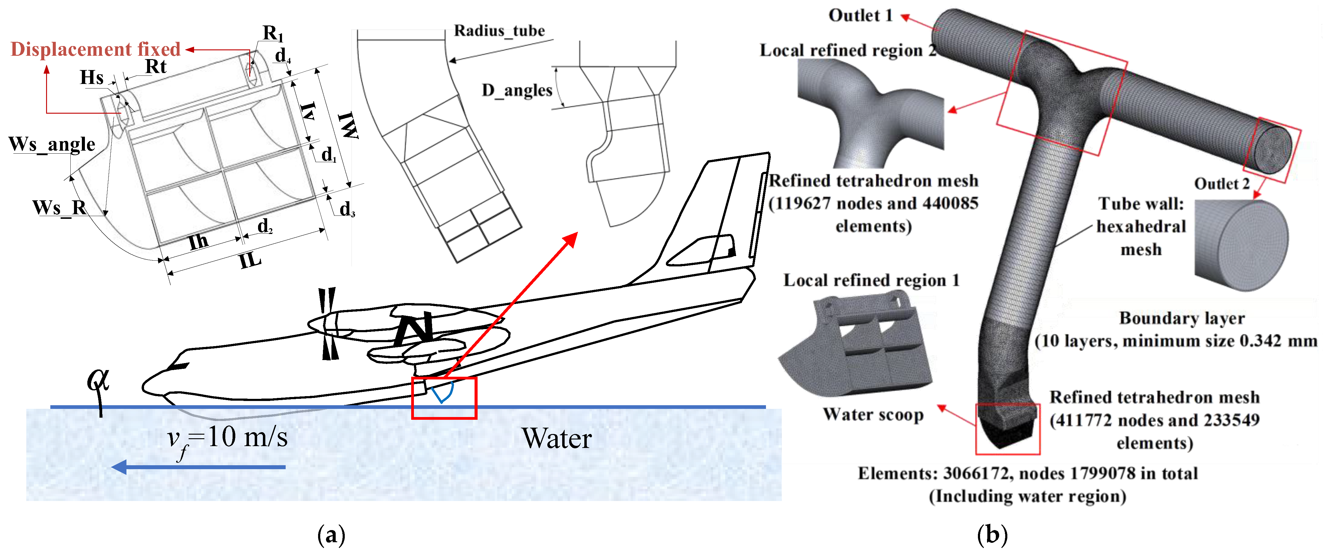
Amphibious aircraft are often used for firefighting by obtaining water from natural lakes or rivers; thus, its water-scooping structure is worth optimizing. Generally, the double-water-scooping buckets locate at the bottom of the fuselage, which join four water tanks by outlet 1 and outlet 2 with tubes, shown in Figure 6. When it works, the amphibious aircraft can put down the scooping buckets and pump water into tanks by skimming quickly over the water surface. In the simulation, the horizontal velocity of the aircraft is vf = 10 m/s and the input angle α = 8°. VBS is used as the development language for the parameterization of the geometric model. The structural parameters are shown in Figure 6a and details can be found in Table 3. In this paper, the commercial software Fluent and Ansys are used for fluid and strength analysis. The water flow is governed by the fluid continuity equation, momentum conservation equation and energy conservation equation. Tetrahedron mesh, which is suitable for iterative optimization due to a higher accuracy and faster convergence speed, is set as the global mesh. Besides, the meshes of key joints and buckets are replaced by the boundary layer mesh, as shown in Figure 6b. The calculation is highly nonlinear and complex, which brings difficulties to ALK modeling.
The initial values come from an existing type of amphibious aircraft, shown in Table 3. A better performance in water scooping heavily depends on the difference in mass flow rate m* between the two outlets. The smaller m* means an optimal efficiency in water pumping. Meanwhile, a maximal equivalent stress should be limited in order to prolong the life cycles. Therefore, m* and σmax are set as the objectives, and the model is
f i n d d ; min Obj = w m m * ( d , P ) + w σ σ max ( d , P ) s . t . d , P Ω g e o h δ s t r u c = max [ δ ( d , P , δ f l u i d ( d , μ X ) ) ] ε d [ d L , d U ]
where Ω g e o is the feasible geometric space for design variables d and normal uncertain parameters P. When conducting the MDO of this model, we firstly establish an initial Kriging model, ALK1 and ALK2, with lower fidelity by learning a small number of samples, e.g., 10 samples, for 2 objects, m* and σmax. One must then judge the convergence condition and obtain the final ALK models. Then, n parallel optimal points d n × m * (m denotes the number of design variables), obtained in the AIC region by optimization algorithms, are selected to train the ALK model until the convergence of relative optimum error ε * is reached.
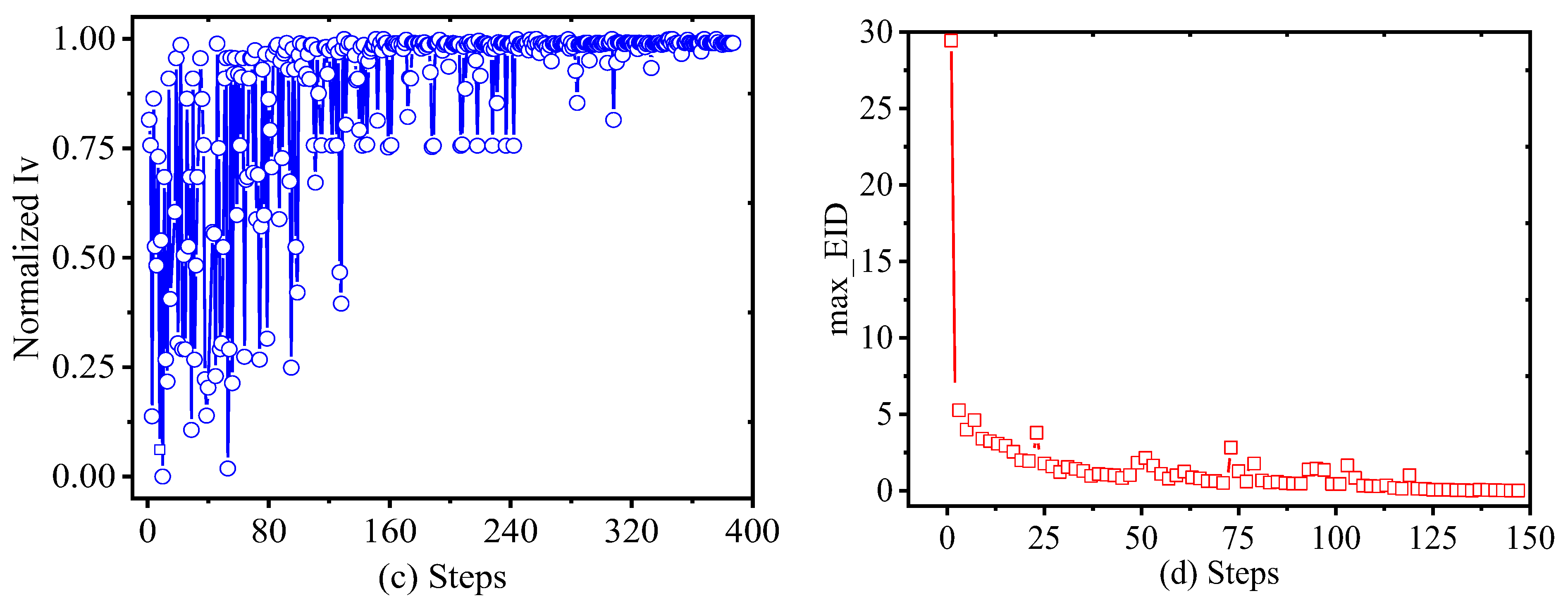
A total of 384 data points of FEM from our previous study has been used for building the direct Kriging model for m* as a comparison. Figure 7a,b show the history of residual convergence of fluid analysis. Figure 7c shows the search history of one design variable Iv by direct FEM. Figure 7d shows the building process for ALK-PAIC.
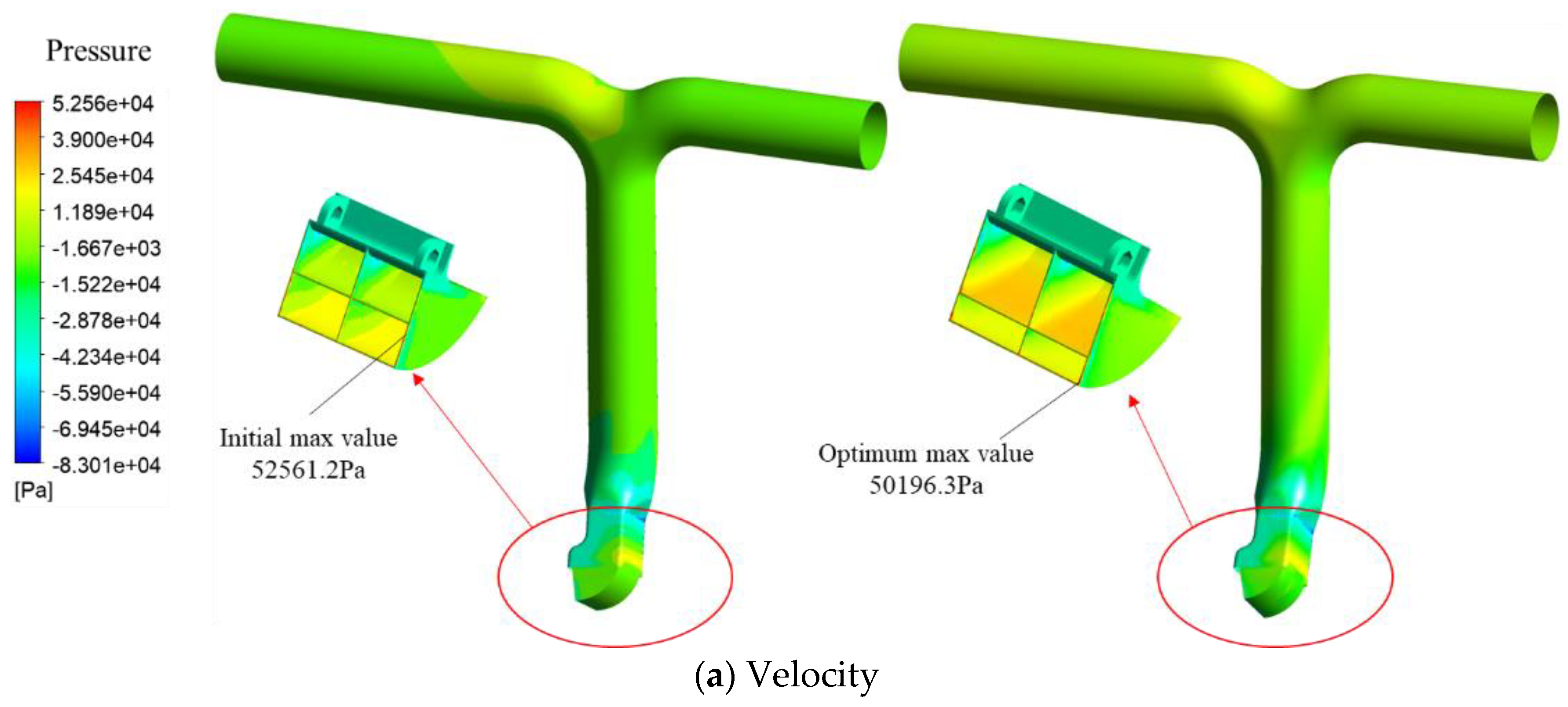
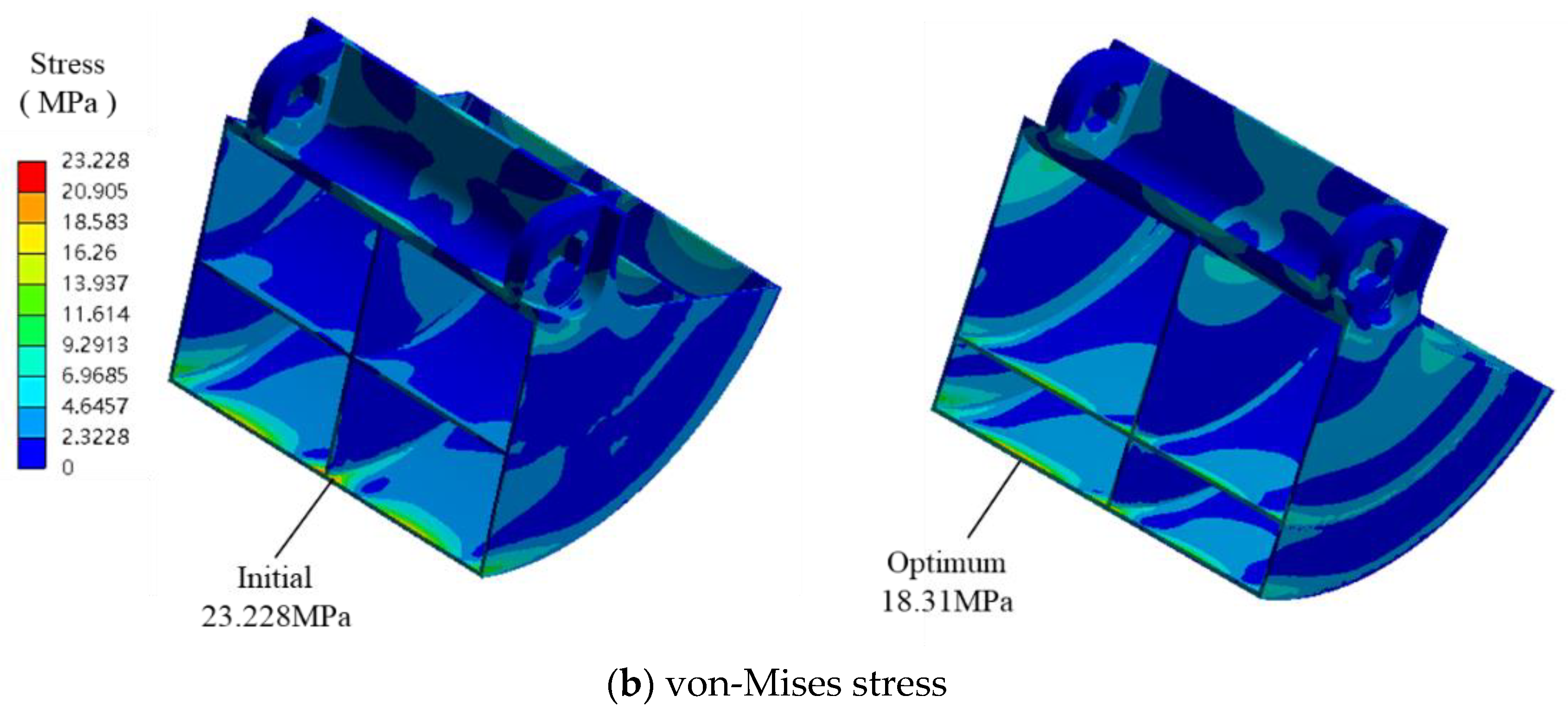
Figure 8a shows the pressure change in optimization, which is obviously that the pressure difference between two outlets becomes smaller after optimization. This is because the water-flow rate distrusted on the bucket surface is not uniform, and the optimization design reassigns the four scoop regions compiled with the nonuniform flow. Figure 8b shows that the stress distribution of the scoop bucket and the σmax are decreased from 23.23 MPa to 18.31 MPa by optimization. The design with the smaller Ws_angle and bigger Iv is safer for the scooping bucket. When the Ws_angle becomes smaller, the normal projection of pressure on the front surface of the scoop becomes strong, leading to a bigger Mises stress. In order to compare the superiority of ALK combined with the EID acquisition function (ALK-EID) with other methods, active radial basis function (RBF) neural networks and direct Kriging with the same accuracy have also been presented here in Table 4. The Kriging model can return the square error of prediction as the important input parameters for the active learning function, while RBF needs extra computation for error analysis. Here, leave-one-out cross validation error analysis Eloo is used for active RBF. Eloo can be obtained by the mean value of repeated p times of cross validation errors with fitted p-1 points by RBF, with one test point. We use p points to build the RBF and p points to obtain the error analysis for active learning training. Therefore, the active RBF model may need more computations compared with ALK. The results in Table 4 show that RBF may perform better in stress prediction than ALK, and the parallel ALK-EGO has the best balance between accuracy and efficiency by adaptively training the most sensitive region.

4. Conclusions

Based on the active learning Kriging (ALK) method, we fully used the returned error analysis by Kriging modelling to form an adaptive changed sample region, called adaptive importance candidate (AIC) region. With the help of parallel techniques influence function (IF), the efficiency of PAIC, with efficient global optimization algorithms, can be improved and has some unique advantages compared with other currently widely used global optimization algorithms. Therefore, the ALK-PAIC method can be used alone as an efficient Bayesian optimization algorithm for complex optimization problems, with multilocal optima, small gradient and implicit objective functions.
Further, it can be modified as a method for searching the most probable failure point (MPP) to solve the reliability problems. Our ALK-PAIC has also demonstrated its performance with higher accuracy and efficiency in multi-mode problems. Specifically, the ALK-PAIC method has potential application in reliability-based multidisciplinary design optimization (RBMDO), with an acceptable computation cost, especially when more sample points are required in small failure probability problems. Although the total number of actual functions calling is almost the same, PAIC can reduce the iteration times with the help of parallel computing compared to the algorithms without parallel methods. Finally, we added an example of MDO for a water-scooping system in an amphibious aircraft to demonstrate its efficiency.

Author Contributions

Conceptualization, M.Z. and Z.Y.; methodology, M.Z. and Z.Y.; software, M.Z.; validation and FEM, Q.Y., X.L. and S.X.; formal analysis, Y.X.; writing—original draft preparation, M.Z.; writing—review and editing, Q.Y.; supervision, Z.Y.; funding acquisition, M.Z., Y.X. All authors have read and agreed to the published version of the manuscript.

Funding

Industrial Development and Foster Project of Yangtze River Delta Research Institute of NPU, Taicang (CY20210201 and CY20210202), and Fundamental Research Funds for the Central Universities under Grant No. G2021KY05114, G2021KY05116.

Institutional Review Board Statement

Not applicable.

Informed Consent Statement

Not applicable.

Data Availability Statement

Not applicable.

Acknowledgments

This work was supported by the Industrial Development and Foster Project of Yangtze River Delta Research Institute of NPU, Taicang (CY20210201 and CY20210202), and Fundamental Research Funds for the Central Universities under Grant No. G2021KY05114, G2021KY05116. The data from the amphibious aircraft were taken from our previous project XXX.

Conflicts of Interest

The authors declare no conflict of interest. The funders had no role in the design of the study; in the collection, analyses, or interpretation of data; in the writing of the manuscript, or in the decision to publish the results.

References

  1. Leimeister, M.; Kolios, A. Reliability-based design optimization of a spar-type floating offshore wind turbine support structure. Reliab. Eng. Syst. Saf. 2021, 213, 107666. [Google Scholar] [CrossRef]
  2. Echard, B.; Gayton, N.; Lemaire, M. AK-MCS: An active learning reliability method combining Kriging and Monte Carlo Simulation. Struct. Saf. 2011, 33, 145–154. [Google Scholar] [CrossRef]
  3. Roshanian, J.; Ebrahimi, M. Latin hypercube sampling applied to reliability-based multidisciplinary design optimization of a launch vehicle. Aerosp. Sci. Technol. 2013, 28, 297–304. [Google Scholar] [CrossRef]
  4. Ni, P.; Li, J.; Hao, H.; Yan, W.; Du, X.; Zhou, H. Reliability analysis and design optimization of nonlinear structures. Reliab. Eng. Syst. Saf. 2020, 198, 106860. [Google Scholar] [CrossRef]
  5. Yang, X.; Mi, C.; Deng, D.; Liu, Y. A system reliability analysis method combining active learning Kriging model with adaptive size of candidate points. Struct. Multidiscip. Optim. 2019, 60, 137–150. [Google Scholar] [CrossRef]
  6. Zhou, Y.; Lu, Z. An enhanced Kriging surrogate modeling technique for high-dimensional problems. Mech. Syst. Signal Process. 2020, 140, 106687. [Google Scholar] [CrossRef]
  7. Zhang, X.; Lu, Z.; Cheng, K. AK-DS: An adaptive Kriging-based directional sampling method for reliability analysis. Mech. Syst. Signal Process. 2021, 156, 107610. [Google Scholar] [CrossRef]
  8. Jones, D.R.; Schonlau, M.; Welch, W.J. Efficient Global Optimization of Expensive Black-Box Functions. J. Glob. Optim. 1998, 13, 455–492. [Google Scholar] [CrossRef]
  9. Bichon, B.J.; Eldred, M.S.; Swiler, L.P.; Mahadevan, S.; McFarland, J.M. Efficient Global Reliability Analysis for Nonlinear Implicit Performance Functions. AIAA J. 2008, 46, 2459–2468. [Google Scholar] [CrossRef]
  10. Yang, X.; Liu, Y.; Gao, Y.; Zhang, Y.; Gao, Z. An active learning kriging model for hybrid reliability analysis with both random and interval variables. Struct. Multidiscip. Optim. 2014, 51, 1003–1016. [Google Scholar] [CrossRef]
  11. Meng, Z.; Zhang, D.; Li, G.; Yu, B. An importance learning method for non-probabilistic reliability analysis and optimization. Struct. Multidiscip. Optim. 2019, 59, 1255–1271. [Google Scholar] [CrossRef]
  12. Song, J.; Wei, P.; Valdebenito, M.A.; Faes, M.; Beer, M. Data-driven and active learning of variance-based sensitivity indices with Bayesian probabilistic integration. Mech. Syst. Signal Process. 2021, 163, 108106. [Google Scholar] [CrossRef]
  13. Zhang, X.; Wang, L.; Sørensen, J.D. REIF: A novel active-learning function toward adaptive Kriging surrogate models for structural reliability analysis. Reliab. Eng. Syst. Saf. 2019, 185, 440–454. [Google Scholar] [CrossRef]
  14. Zhang, M.; Yao, Q.; Sun, S.; Li, L.; Hou, X. An efficient strategy for reliability-based multidisciplinary design optimization of twin-web disk with non-probabilistic model. Appl. Math. Model. 2020, 82, 546–572. [Google Scholar] [CrossRef]
  15. Viana, F.; Haftka, R.T.; Steffen, V. Multiple surrogates: How cross-validation errors can help us to obtain the best predictor. Struct. Multidiscip. Optim. 2009, 39, 439–457. [Google Scholar] [CrossRef]
  16. Wen, Z.; Pei, H.; Liu, H.; Yue, Z. A Sequential Kriging reliability analysis method with characteristics of adaptive sampling regions and parallelizability. Reliab. Eng. Syst. Saf. 2016, 153, 170–179. [Google Scholar] [CrossRef]
  17. Yun, W.; Lu, Z.; He, P.; Dai, Y.; Feng, K. Adaptive subdomain sampling and its adaptive Kriging–based method for reliability and reliability sensitivity analyses. Struct. Multidiscip. Optim. 2020, 61, 1107–1121. [Google Scholar] [CrossRef]
  18. Sóbester, A.; Leary, S.J.; Keane, A.J. A parallel updating scheme for approximating and optimizing high fidelity computer simulations. Struct. Multidiscip. Optim. 2004, 27, 371–383. [Google Scholar] [CrossRef] [Green Version]
  19. Wang, Z.; Wang, P. A double-loop adaptive sampling approach for sensitivity-free dynamic reliability analysis. Reliab. Eng. Syst. Saf. 2015, 142, 346–356. [Google Scholar] [CrossRef]
  20. Meng, Z.; Keshtegar, B. Adaptive conjugate single-loop method for efficient reliability-based design and topology optimization. Comput. Methods Appl. Mech. Eng. 2019, 344, 95–119. [Google Scholar] [CrossRef]
  21. Meng, D.; Li, Y.-F.; Huang, H.-Z.; Wang, Z.; Liu, Y. Reliability-based multidisciplinary design optimization using subset simulation analysis and its application in the hydraulic transmission mechanism design. J. Mech. Des. 2015, 137, 051402. [Google Scholar] [CrossRef]
  22. Fei, C.-W.; Li, H.; Liu, H.-T.; Lu, C.; Keshtegar, B.; An, L.-Q. Multilevel nested reliability-based design optimization with hybrid intelligent regression for operating assembly relationship. Aerosp. Sci. Technol. 2020, 103, 105906. [Google Scholar] [CrossRef]
  23. Wang, L.; Xiong, C.; Hu, J.; Wang, X.; Qiu, Z. Sequential multidisciplinary design optimization and reliability analysis under interval uncertainty. Aerosp. Sci. Technol. 2018, 80, 508–519. [Google Scholar] [CrossRef]
  24. Song, L.-K.; Bai, G.-C.; Li, X.-Q. A novel metamodeling approach for probabilistic LCF estimation of turbine disk. Eng. Fail. Anal. 2021, 120, 105074. [Google Scholar] [CrossRef]
  25. Melchers, R.; Ahammed, M. A fast approximate method for parameter sensitivity estimation in Monte Carlo structural reliability. Comput. Struct. 2004, 82, 55–61. [Google Scholar] [CrossRef]
  26. Zhang, M.; Yao, Q.; Sheng, Z.; Hou, X. A sequential reliability assessment and optimization strategy for multidisciplinary problems with active learning kriging model. Struct. Multidiscip. Optim. 2020, 62, 2975–2994. [Google Scholar] [CrossRef]
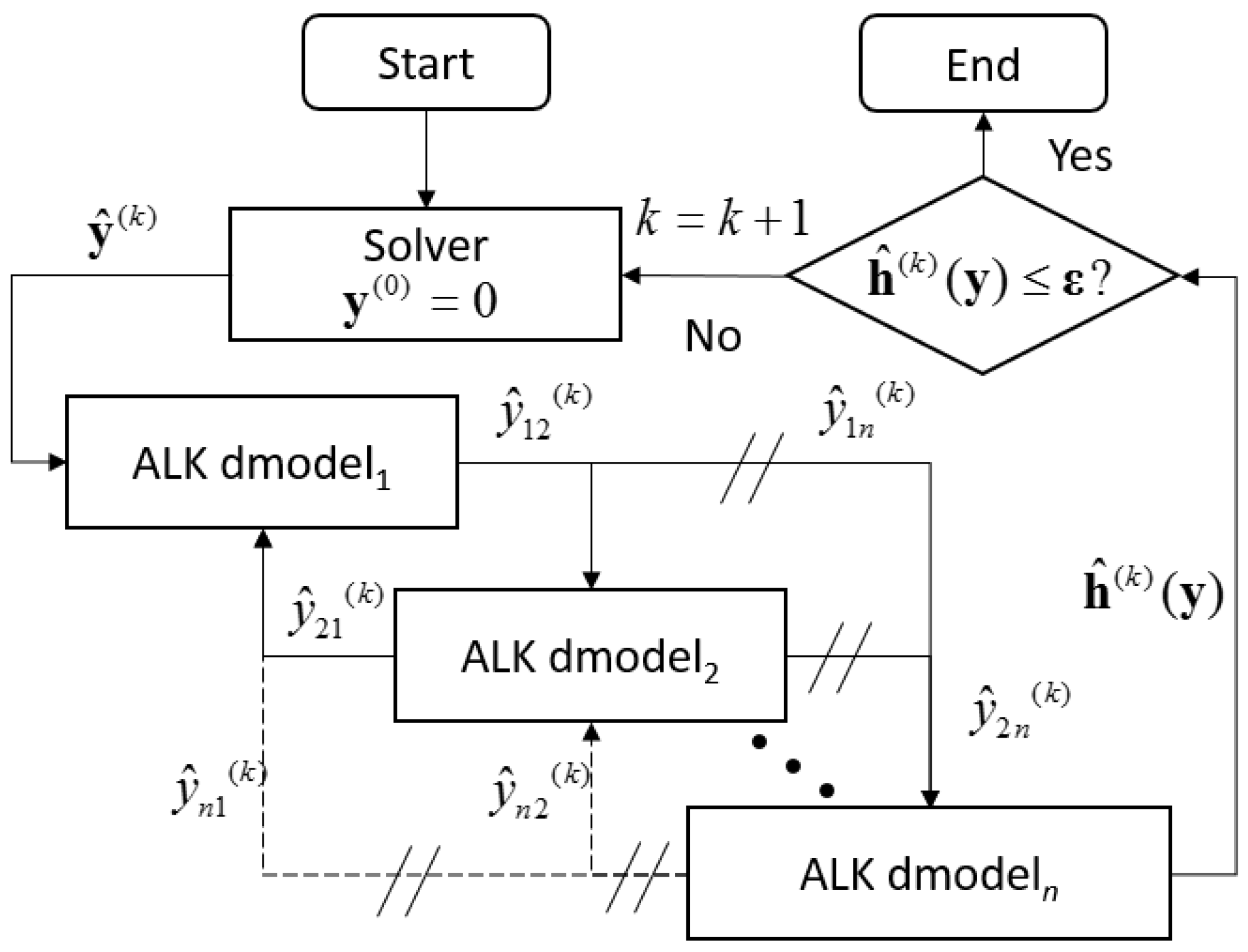
Figure 1. The process of the multidisciplinary feasible method (MDF).
Aerospace 09 00240 g001
Figure 2. Search history of double-peak function by (a) Original function, (b) Predictive function by EID, (c) Predictive function by EIE, (d) Predictive function by AIC, (e) Predictive function by PAIC, where asterisk (*) denotes the original points, square (□) denotes the additional training points, red dot denotes the predictive global optimum.
Aerospace 09 00240 g002
Figure 3. Search history of MPP for the four branches case by (a) AIC β = 1.8, (b) shows the figure of zooming on the AIC regions. (c) The results without AIC method. (d) Shows parallel total training by PAIC (ACR means the active candidate region in AIC methods).
Aerospace 09 00240 g003aAerospace 09 00240 g003b
Figure 4. Dynamic np change in each iteration.
Aerospace 09 00240 g004
Figure 5. The searching history figures of multi-mode case by SORA. (a) No AIC ds = 0.5; (b) PAIC ds = 0.5; (c) PAIC ds = 1.2; (d) Zoom on (PAIC ds = 1.2). The five-pointed star denotes the real optimum.
Aerospace 09 00240 g005
Figure 6. The schematic graph of scooping system in amphibious aircraft. (a) Structure; (b) Mesh.
Aerospace 09 00240 g006
Figure 7. Search history of involved parameters in optimization.
Aerospace 09 00240 g007aAerospace 09 00240 g007b
Figure 8. The comparison between initial point and optimal point.
Aerospace 09 00240 g008aAerospace 09 00240 g008b
Table 1. The results of four branches case by different methods.
MethodsAvg. NAvg. NaddAvg. IterAvg. NpAvg. PfAvg. |εf|
MCS1.0 × 109///1.218 × 10−5/
1.0 × 10⁷///1.220 × 10−51.642 × 10−3
EGRA116.25106.25116.25/1.275 × 10−54.680 × 10−2
K-MCS (nMC = 1.0 × 10⁷)765.12755.12755.12/1.240 × 10−51.806 × 10−2
ALK-MCS (nMC = 1.0 × 10⁷)116.25106.25116.25/1.176 × 10−53.448 × 10−2
ISKRA (K-m × 10 ans)115.8105.817.6361.170 × 10−53.941 × 10⁻²
ALK-PAIC (nMC = 1.0 × 10⁷)86.4776.4211.656.561.192 × 10−52.135 × 10⁻²
ALK-PAIC (nMC = 1.0 × 10⁵)86.4776.4211.656.561.165 × 10−54.351 × 10⁻²
ALK-PAIC (IS)86.4776.4211.656.561.158 × 10−54.926 × 10⁻²
Table 2. The optimum point with systemic reliability constraints predicted by different models (n is original number, m is number of adding points).
ALK MethodsNOBF
n + (m)
Avg. NLSF
n + (m)
Step Length
ds
Avg. Iter.εOptimal ValueOptimal Points
x1x2
ERF-PAIC10 + (10)20 + (35.12)0.515.1510−51.37464.26132.8257
ERF-PAIC10 + (10)20 + (39.65)0.520.9410−81.37494.25922.8281
ERF-PAIC10 + (10)20 + (26.23)1.210.5010−51.37484.26082.8261
ERF-AIC10 + (10)20 + (27.45)1.267.4510−51.37514.26172.8251
ERF10 + (10)20 + (39.10)1.279.1010−51.37524.26182.8249
/151151 × 106///1.37504.26152.8225
Table 3. Parameters, design variables and objectives involved in optimization.
TypeSymbolDescriptionUnitLower
Limits
Initial ValueUpper Limits
Parameters
P
(normal distribution, σ = 0.5%)
Ws_RRadius of scoopmm/260/
R1Radius of scoop rotary shaft ribsmm/20/
IWInlet height of water scoopmm/116.8/
ILLength of scoopmm/166/
RtThickness of scoop rotary shaft ribsmm/10/
HsLength of the side of hexagonmm/11.5/
d1Thickness of horizontal bafflemm/2/
d2Thickness of vertical bafflemm/2/
d3Thickness of lower bordermm/2/
d4Thickness of the upper bordermm/2/
Design variables
d
Radius_tubeRadius of tube bendmm225250275
IvDistance from the horizontal baffle to the upper border of scoopmm54.46881.6
IhDistance from the vertical baffle to the left border of scoopmm648096
D_anglesIncluded angle between section of scooping bucket and tube°−8.547−7.77−6.216
Ws_angleIncluded angle between inlet and outlet of scoop°72.98189.1
Objectivesm*Mass flow difference between two outletskg/s///
σmaxMax Mises stress in water scoopingMPa///
Table 4. The comparison between the initial and optimal designs.
InitialGA with Direct FEMRBF-AIC with EGOKriging with EGOParallel ALK-AIC with EGO
ValueCR (%)ValueError (%)ValueError (%)ValueError (%)
Radius_tube (mm)250225.81↓9.676226.510.310227.910.930227.250.638
Iv (mm)6881.328↑19.60081.131−0.24281.4210.11481.187−0.173
Ih (mm)8085.675↑7.09485.7610.10085.7330.06887.5762.219
D_angles (°)8174.25↓8.33374.2800.04074.2880.05174.058−0.259
Ws_angle (°)−7.77−6.802↓12.458−6.9452.102−6.9281.852−6.8−0.029
m* (kg/h)70.01812.491↓82.16015.9111.36015.6689.42311.564−7.421
Max_stress (MPa)23.22817.75↓23.58416.493−7.08215.073−15.08218.313.155
Number of iterations/401 (401 samples)185 (195 samples)374 (384 samples)148 (190 samples)
Max_EID//0.00910.01000.0097
Publisher’s Note: MDPI stays neutral with regard to jurisdictional claims in published maps and institutional affiliations.