Case Study for Testing the Validity of NO_x-Ozone Algorithmic Climate Change Functions for Optimising Flight Trajectories

Abstract

One possibility to reduce the climate impact of aviation is the avoidance of climate-sensitive regions, which is synonymous with climate-optimised flight planning. Those regions can be identified by algorithmic Climate Change Functions (aCCFs) for nitrogen oxides (NO${}_x$), water vapour (H${}_2$O) as well as contrail cirrus, which provide a measure of climate effects associated with corresponding emissions. In this study, we evaluate the effectiveness of reducing the aviation-induced climate impact via ozone (O${}_3$) formation (resulting from NO${}_x$ emissions), when solely using O${}_3$ aCCFs for the aircraft trajectory optimisation strategy. The effectiveness of such a strategy and the associated potential mitigation of climate effects is explored by using the chemistry–climate model EMAC (ECHAM5/MESSy) with various submodels. A summer and winter day, characterised by a large spatial variability of the O${}_3$ aCCFs, are selected. A one-day air traffic simulation is performed in the European airspace on those selected days to obtain both cost-optimised and climate-optimised aircraft trajectories, which more specifically minimised a NO${}_x$-induced climate effect of O${}_3$ (O${}_3$ aCCFs). The air traffic is laterally and vertically re-routed separately to enable an evaluation of the influences of the horizontal and vertical pattern of O${}_3$ aCCFs. The resulting aviation NO${}_x$ emissions are then released in an atmospheric chemistry–climate simulation to simulate the contribution of these NO${}_x$ emissions to atmospheric O${}_3$ and the resulting O${}_3$ change. Within this study, we use O${}_3$-RF as a proxy for climate impact. The results confirm that the climate-optimised flights lead to lower O${}_3$-RF compared to the cost-optimised flights, although the aCCFs cannot reproduce all aspects of the significant impact of the synoptic situation on the transport of emitted NO${}_x$. Overall, the climate impact is higher for the selected summer day than for the selected winter day. Lateral re-routing shows a greater potential to reduce climate impact compared to vertical re-routing for the chosen flight altitude. We find that while applying the O${}_3$ aCCFs in trajectory optimisation can reduce the climate impact, there are certain discrepancies in the prediction of O${}_3$ impact from aviation NO${}_x$ emissions, as seen for the summer day. Although the O${}_3$ aCCFs concept is a rough simplification in estimating the climate impact of a local NO${}_x$ emission, it enables a reasonable first estimate. Further research is required to better describe the O${}_3$ aCCFs allowing an improved estimate in the Average Temperature Response (ATR) of O${}_3$ from aviation NO${}_x$ emissions. A general improvement in the scientific understanding of non-CO${}_2$ aviation effects could make climate-optimised flight planning practically feasible.

1. Introduction

Reducing anthropogenic climate change is one of the most significant existential challenges that we face, and it requires a strong global response to, e.g., avoid tipping points [1]. Aviation, for instance, contributed to 3.5% of anthropogenic climate change in terms of Effective Radiative Forcing when contrail-cirrus effects were included [2] and 5% in terms of temperature change [3]. Aviation climate impact is expected to grow rapidly due to the growth of the air transport sector in most regions of the world. The 4.3 billion airline passengers carried in 2018 are expected to grow to about 10 billion by 2040, and the number of departures is projected to rise to some 90 million in 2040 [4]. Airbus [5], in its Global Market Forecast, predicts a continued annual growth rate of 4.4% in revenue passenger kilometres for the next two decades. Boeing [6], in its Commercial Market Outlook, expects an annual growth rate of 4.6% per year. The effects of the COVID-19 pandemic are expected to only have a temporary effect on this growth [3].

Although efforts have been made to reduce fuel consumption (and hence reduce the CO${}_2$ emissions) with technological, operational and regulatory measures, they are not sufficient to tackle the overall climate impact of aviation. This is because non-CO${}_2$ emissions from engine fuel combustion contribute to about 2/3 of the warming [2] in terms of Radiative Forcing (RF) with large uncertainties for contrail-cirrus effects. The most important non-CO${}_2$ emissions include persistent line-shaped contrails, contrail-induced cirrus clouds and nitrogen oxide (NO${}_x$ = NO + NO${}_2$) emissions that alter the O${}_3$ and CH${}_4$ concentrations, both of which are greenhouse gases, and the emission of water vapour (H${}_2$O).

It is important to understand the fundamental differences between CO${}_2$ and non-CO${}_2$ effects in order to predict the overall climate impact of aviation. The climate impact of CO${}_2$ is proportional to the quantity of CO${}_2$ released during the flight and, as CO${}_2$ is a long-lived and relatively well-mixed gas, the impact is independent of the emission location. Additionally, the climate impact of CO${}_2$ has been determined with a high confidence level. On the contrary, non-CO${}_2$ emissions and contrail cirrus have shorter atmospheric residence times and are heterogeneously distributed. For each non-CO${}_2$ emission, it is not just the individual concentration that is important but also the location of the emission, the associated timescale, chemical background condition, etc. [7,8,9]. Consequently, the confidence levels are much lower and associated uncertainties are much higher for these non-CO${}_2$ effects (Figure 3 of [2]).

Because non-CO${}_2$ effects show strong spatial and temporal variations, the weather situation and subsequent transport pathways play a major role in their climate impact. Accordingly, operational measures such as climate-optimised flight planning can be enforced to avoid regions where these impacts are substantial. This was the primary motivation behind the Reducing Emissions from Aviation by Changing Trajectories for the benefit of Climate (REACT4C, https://www.react4c.eu/, accessed on 20 October 2021) project [10]. The project led to the development of Climate Change Functions (CCFs, [9,11]) that can quantify the climate impact for a unit emission at a given longitude, latitude, altitude and time. The effects take into account the CO${}_2$ emissions and non-CO${}_2$ effects from the NO${}_x$ and H${}_2$O emissions and contrail formation. The CCFs describe “climate sensitive regions” which are 4D regions in space-time, indicating where aviation emissions have a larger impact on climate change in comparison to other regions. The CCFs were used in an air traffic optimisation routine to avoid climate-sensitive regions and quantitatively showed a reduction potential of up to 25% in climate impact for a small increase in cost (0.5%, [12]). However, these results were computationally intensive to generate in the first place and also restricted to the Trans-Atlantic airspace. This makes the practical use of these tools in climate-optimised flight planning a major obstacle. As a following step, a more general and practical tool was sought while making use of the vast amount of CCFs data, which was one of the objectives of the Air Traffic Management 4 Environment (ATM4E, https://www.atm4e.eu/, accessed on 20 October 2021) project. Among other things, this project explored the feasibility of a concept for environmental assessment of ATM operations working towards environmental optimisation of air traffic operations in the European airspace [13]. The project led to the development of algorithmic Climate Change Functions (aCCFs) separately for the NO${}_x$ effect on O${}_3$ (NO${}_x$-O${}_3$) and methane (NO${}_x$-CH${}_4$) (Sections 4.3 and 4.5 of [14], respectively), water vapour (H${}_2$O) (Section 3.3 of [14]) and contrail cirrus [15], and the aCCFs are implemented as a submodel [16] in the ECHAM5/MESSY Atmospheric Chemistry (EMAC) model [17]. These formulas, obtained using regression techniques, are computationally inexpensive, fairly general and provide the climate impact based on meteorological inputs, in terms of a metric called F-ATR20 which gives the Average Temperature Response over a time horizon of 20 years given future increasing emissions (e.g., Fa1 scenario, [18]). With these salient properties, the prototype aCCFs are expected to be used to optimise flight trajectories (in real time) with respect to its overall climate impact (CO${}_2$ and non-CO${}_2$) and also to estimate the climate impact of individual flight trajectories. A general comparison between the characteristics of the CCFs and aCCFs is listed in

Table 1. Comparison of crucial characteristics of CCFs and aCCFs. “NWPs” stands for numerical weather prediction models.

Parameters	CCFs	aCCFs
Weather	Five specific winter days and three specific summer days	Arbitrary days
Geographical applicability	North Atlantic region	30–90° N
Practical implementation	Limited due to expensive computations	Easily implemented in NWPs
Verification process	Comparison of general patterns with literature	Climate–chemistry model simulation with flight optimisation tool

.

The quality of the aCCFs are expressed in terms of the adjusted $R^2$ [19]. This value is large for H${}_2$O aCCFs, but for O${}_3$ aCCFs and CH${}_4$ aCCFs, it is much smaller [14]. A strict verification process for the aCCFs is required in general and this study focuses specifically on the O${}_3$ aCCFs evaluation.

NO${}_x$ (=NO + NO${}_2$) is an indirect greenhouse gas that leads to a short-term increase in tropospheric O${}_3$ production (warming) and a long-term increase in CH${}_4$ oxidation (cooling) in the atmosphere. Because CH${}_4$ is a precursor for changes in O${}_3$, a long-term reduction in O${}_3$ called the primary mode ozone (PMO) effect [20] occurs due to CH${}_4$ oxidation, resulting in cooling. Additionally, less CH${}_4$ enters the stratosphere, where it is decomposed into CO${}_2$ and H${}_2$O. Eventually, this reduces the stratospheric water vapour (SWV), resulting in cooling [21]. However, the net climate effect for this chain of reactions is warming [22,23,24]. The short-term O${}_3$ production from NO${}_x$ starts with the formation of NO${}_2$ from NO through the reaction with HO${}_2$. Through photolysis of NO${}_2$, O(${}^3$P) is formed which in turn forms O${}_3$. Therefore, the following reactions are included:

$${\mathrm{HO}}_2+\mathrm{NO}\to \mathrm{OH}+{\mathrm{NO}}_2$$

(1)

$${\mathrm{NO}}_2\stackrel{\mathrm{h}\nu }{\to }\mathrm{NO}+\mathrm{O}{(}^3\mathrm{P})$$

(2)

$$\mathrm{O}{(}^3\mathrm{P})+{\mathrm{O}}_2\to {\mathrm{O}}_3$$

(3)

For further details on the chain of chemical reactions relating to CH${}_4$, the reader is referred to Rosanka et al. [25]. The NO${}_x$ effects are characterised by significant seasonal and spatial variability due to the dependence on incoming solar radiation and background chemical (especially NO${}_x$) concentrations [26]. Frömming et al. [9] found that not only the emission region is relevant; in fact, the main driver for the enhanced climate sensitivity is the transport pathways of emissions within the first week(s) after emissions are released. The transport pathways are in turn driven by the meteorological situation. The detailed impact of weather patterns and related transport processes on aviation’s contribution to O${}_3$ is also reported by Rosanka et al. [25].

Preliminary results by Yin et al. [27] showed that climate-optimised flight trajectories considering only O${}_3$ aCCFs reduce the NO${}_x$-induced O${}_3$ RF. Here, we are aiming to extend it by following a more detailed optimisation procedure (treating lateral and vertical shifts) involving a large variability of O${}_3$ aCCFs. Hartjes et al. [28] determined three-dimensional aircraft trajectories while minimizing contrail formation. They found vertical trajectory adjustments to be preferable over horizontal trajectory changes. This is an additional motivation to separately investigate the impact of lateral re-routing and vertical re-routing in relation to NO${}_x$-O${}_3$ effects. As a result, it is possible to analyse different NO${}_x$ emission profiles emerging from cost and climate-optimised simulations on days characterised by a large variability of O${}_3$ impact. In order to test the ability to use the O${}_3$ aCCFs for a reduction in O${}_3$-RF by trajectory optimisation, a summer day and a winter day characterised by a large variability of O${}_3$ impact are selected. Subsequently, the atmospheric transport subject to meteorology and climate impact is analysed for all cases which are discussed in Section 3. This leads to information on the viability of the O${}_3$ aCCFs as a tool for obtaining climate-friendly trajectories as well as the impact of lateral and vertical re-routing.

The present study is organised as follows: In Section 2, we give an overview of the model system used and describe the applied setup in Section 3. In Section 4, we analyse our simulation results with respect to the contribution of NO${}_x$ emissions from lateral re-routing and vertical re-routing on two selected days to tropospheric O${}_3$ production and the resulting climate impact in terms of O${}_3$-RF. Here, a direct comparison of the climate impact from cost-optimised and O${}_3$ aCCFs-optimised trajectories is made. In Section 5, we discuss and conclude the present study.

2. Methodology

2.1. EMAC Model and Used Submodels

The ECHAM/MESSy Atmospheric Chemistry (EMAC) model is a numerical chemistry and climate simulation system that includes submodels describing tropospheric and middle atmosphere processes and their interaction with oceans, land and human influences [17]. It uses the second version of the Modular Earth Submodel System (MESSy, [17]) to link multi-institutional computer codes. The core atmospheric model is the 5th generation European Centre Hamburg general circulation model (ECHAM5) developed by the Max Planck Institute for Meteorology [29,30] and the chemistry is simulated by MECCA (version 3.2, [31]) in the gas phase and SCAV [32] in the aqueous phase. For the present study, we applied EMAC (ECHAM5 version 5.3.02, MESSy version 2.54.0) with the T42L31ECMWF resolution, corresponding to a quadratic Gaussian grid of 2.8 by 2.8° in latitude and longitude and 31 vertical hybrid pressure levels up to 10 hPa (an altitude of roughly 30 km). The vertical resolution at flight levels is roughly 1 km and the simulation time step is 12 min. MESSy provides interfaces to couple various submodels of EMAC. Figure 1 shows the current model setup where the main submodels used are ACCF 1.0 [16], AirTraf 2.0 [33], TAGGING 1.1 [34] and RAD [35], which are described in subsequent sections. The complete list of used EMAC submodels in this study can be found in

Table A1. List of EMAC submodels used in the simulations.

Submodel	Purpose	Reference
AEROPT	Aerosol optical properties for the radiation scheme	[35]
ACCF 1.0	Climate impact of aviation emissions and contrails calculation	[16]
AIRTRAF 2.0	Air traffic simulation	[33]
CH4 1.0	Simple methane chemistry	[65]
CLOUD	Standard ECHAM5 cloud microphysics calculation	[30]
CLOUDOPT	Cloud optical properties calculation for the radiation scheme	[35]
CVTRANS	Calculates the transport of tracers due to convection	[66]
CONVECT	Convection process calculation	[67]
CONTRAIL	Contrail potential coverage calculation	Supplement of [12,68]
DDEP	Dry deposition of gas phase and aerosol tracers	[69]
E5VDIFF	ECHAM5 vertical diffusion and land-atmosphere exchange	[17]
GWAVE	Gravity waves calculation	[17]
JVAL	Photolysis rates	[70]
LNOX	Lighting NO${}_x$ production	[71]
MSBM	Multi-phase stratospheric box model calculates the heterogeneous reaction rates on polar stratospheric cloud particles and stratospheric background aerosols	[17]
MECCA	Calculates tropospheric and stratospheric chemistry	[31]
O3ORIG	To trace the origin of ozone	[72]
OFFEMIS	Prescribed emissions of trace gases and aerosols	[73]
ONEMIS	Online calculated emissions of trace gases and aerosols	[73]
ORBIT	Earth orbit calculation for solar zenith angle, etc.	[35]
RAD	Simulates the radiative flux	[35]
SCAV	Simulates the process of wet deposition and liquid phase chemistry	[32]
SCALC	Simple calculations with channel objects to separate the AirTraf ozone from other ozone sources	[17]
SEDI	Sedimentation of aerosol particles	[69]
SURFACE	Calculates the surface temperature	[17]
TAGGING 1.1	Tag the emissions contributions to concentrations	[34]
TNUDGE	Tracer nudging	[73]
TROPOP	Tropopause and other diagnosis	[74]

of Appendix A.

2.2. The Algorithmic Climate Change Functions Submodel: ACCF

The planning of climate-optimised flight trajectories requires the knowledge of the climate impact of a local emission, i.e., climate-sensitive regions. This information is provided by the aCCFs which represent a correlation of the synoptic situation at the time of emission and the respective CCFs, which can easily be implemented in any numerical weather prediction model (NWP). Currently, the submodel ACCF (version 1.0, [16]) has been developed that contains the prototype aCCFs for CO${}_2$, NO${}_x$-O${}_3$, NO${}_x$-CH${}_4$, H${}_2$O and contrail cirrus. The ACCF submodel is coupled with the AirTraf submodel (Section 2.3) for climate-optimised trajectory optimisations.

Here, we use the O${}_3$ aCCFs [14] as implemented in EMAC via the ACCF submodel. Van Manen and Grewe [14] have tested a wide range of parameters that influence the impact of NO${}_x$ on O${}_3$, such as the synoptic situation, solar radiation, chemical background condition and lightning indicators, and found that meteorological variables such as temperature and geopotential were the most influential factors for predicting the temporal change in O${}_3$. Ultimately, the O${}_3$ aCCFs for an atmospheric location $(x,y,z)$ at time t with temperature $T=T(x,y,z,t)$ and geopotential $\Phi =\Phi (x,y,z,t)$ was given by,

$$\begin{array}{c}\hfill \begin{array}{cc}\hfill {\mathrm{aCCF}}_{{\mathrm{O}}_3}(T,\Phi )=& -5.20\times {10}^{-11}+\left(2.30\times {10}^{-13}\right)T+\left(4.85\times {10}^{-16}\right)\Phi \hfill \\ \hfill & -\left(2.04\times {10}^{-18}\right)T\Phi .\hfill \end{array}\end{array}$$

(4)

If a certain input $(T,\Phi )$ results in a negative value for Equation (4), the result is converted to zero, since no cooling effect is expected from O${}_3$ production. An example of O${}_3$ aCCFs is shown in Figure 2 for an arbitrary weather situation, where a clear connection is seen between the two panels in terms of the patterns. In general, higher values of temperature and geopotential are associated with higher values of O${}_3$ aCCFs.

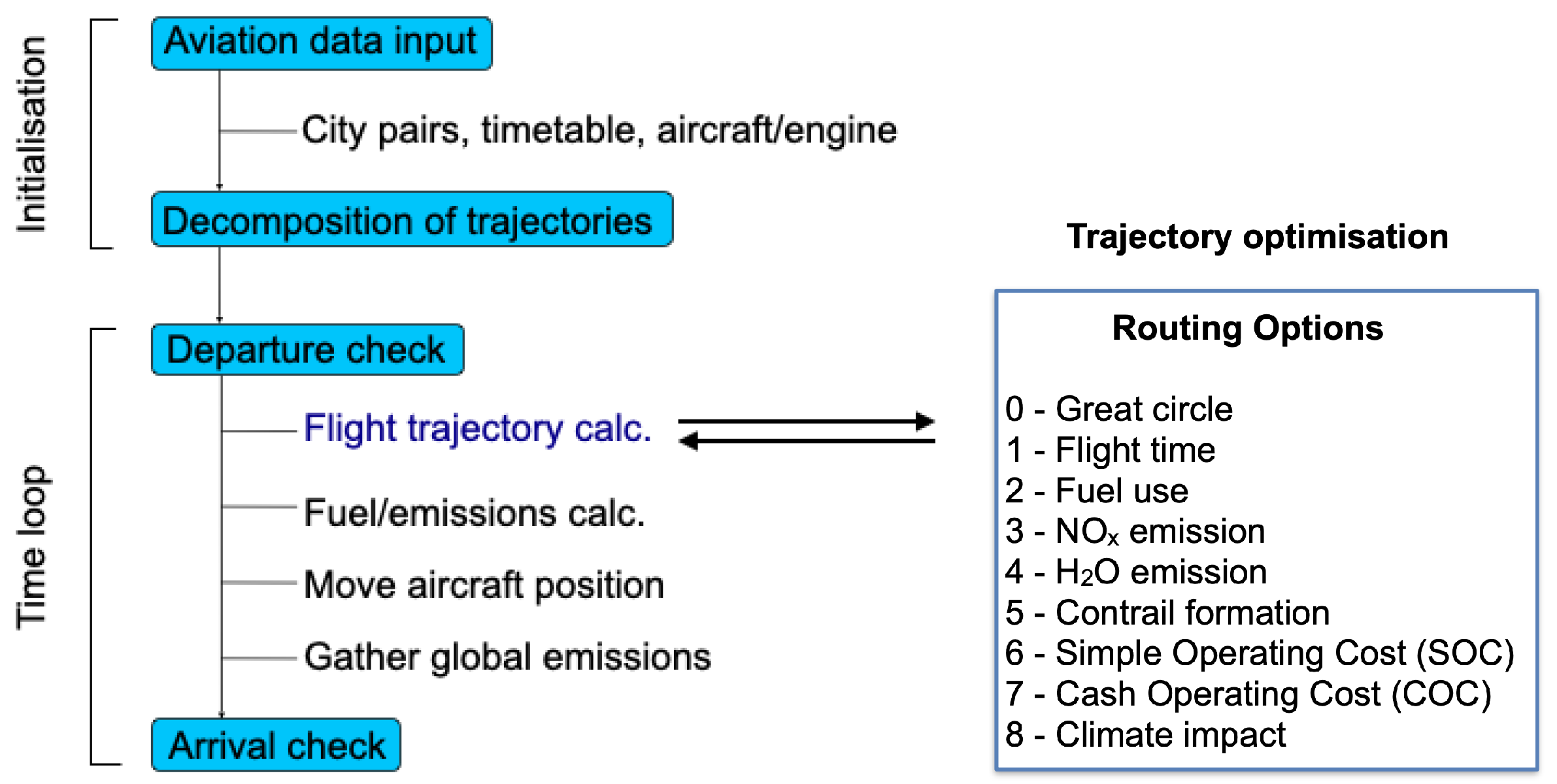
2.3. The Air Traffic Simulator Submodel: AirTraf

AirTraf 2.0 [33] is a global 3D air traffic simulation tool which is implemented in EMAC as a submodel. This submodel has various optimisation objectives, as shown in Figure 3, and can take into account effects of local weather conditions (e.g., wind) during air traffic optimisation. The air traffic information comprises the Eurocontrol’s Base of Aircraft Data (BADA Revision 3.9, [36]) aircraft performance model and the International Civil Aviation Organization (ICAO) [37] emission data bank. Fuel use and NO${}_x$ emissions are calculated by the total energy model based on the BADA methodology [38] and the DLR (Deutsches Zentrum für Luft- und Raumfahrt) fuel flow method [39]. The flight trajectory optimisation is performed by the Adaptive Range Multi-Objective Genetic Algorithm (ARMOGA version 1.2.0, [40,41,42]).

Figure 3 shows the AirTraf procedure. First, air traffic data are required, which consist of a 1-day flight plan of city pairs and the departure times. Additionally, aircraft and engine performance data are also provided. For all optimisation objectives, the local weather conditions are provided by online calculation of ECHAM5. The optimised trajectory is dependent on setting certain bounds for design variables. There are eleven design variables in total for the geometry definition of a flight trajectory, five of which are altitude-related (vertical cross section) and six are related to the latitude and longitude (horizontal cross section), as shown in Figure 4. These variables can be adjusted by the user according to the type of re-routing that is desired, which will be explained in Section 3.2. Following the flight trajectory calculation, fuel use and NO${}_x$ emissions are calculated. Subsequently, aircraft positions are advanced along the flight trajectory corresponding to the time steps of EMAC. Finally, the individual aircraft’s emissions corresponding to the flight path in one time step are gathered into a global field. The flying process ends when the arrival check is passed.

2.4. Contribution of Emissions to Concentrations Submodel: TAGGING

The assessment of the contribution of individual emissions of precursors on climate necessitates a detailed analysis of the chemical conversion, transport and deposition of these species in numerical chemistry climate simulations. A frequently used method for this is called tagging and a generalised approach is described by Grewe [45]. The objective of the tagging scheme is to determine the contribution of emissions from various sectors. For instance, NO${}_x$ is a precursor of tropospheric O${}_3$ but has several anthropogenic emission sources, such as road traffic, shipping, industry and air traffic, and non-anthropogenic sources, such as lightning, emissions from soils, etc. Working like an accounting system, we create a new category specifically for NO${}_x$ emissions emerging from AirTraf. We can then answer the question, “What is the contribution of air traffic emissions to O${}_3$ mixing ratios and corresponding RF?” The tagging approach is implemented as a submodel (TAGGING 1.1, [34,46]) within MESSy.

2.5. Radiation Infrastructure Submodel: RAD

RF is the annual change in energy flux in the atmosphere caused by atmospheric composition changes as measured in W/m${}^2$ [47]. It is a widely used metric to quantify and compare the external drivers of changes to the Earth’s energy balance. RF calculations are implemented by the submodel RAD [35] within MESSy. The RF of O${}_3$ perturbations is defined as the difference in the net radiative fluxes caused by a change (e.g., between two time periods such as pre-industrial and present day; [47]). Here, we are interested in the contribution of AirTraf NO${}_x$ emissions (atf) to this RF. In order to do this, we calculate the full O${}_3$ contribution from all emission sources and subtract contributions from all sources with the exception of AirTraf (non-atf) using the EMAC submodel SCALC (Table A1). That is,

$$\mathrm{RF}\left({\mathrm{O}}_3\mathtt{atf}\right)=\mathrm{RF}\left({\mathrm{O}}_3\right)-\mathrm{RF}({\mathrm{O}}_3\mathtt{non}-\mathtt{atf})$$

(5)

This approach is consistent with the IPCC RF definition, since the sum of all individual RF contributions approximately equals the total RF (for a detailed example, see Dahlmann et al. [48] and Mertens et al. [49]).

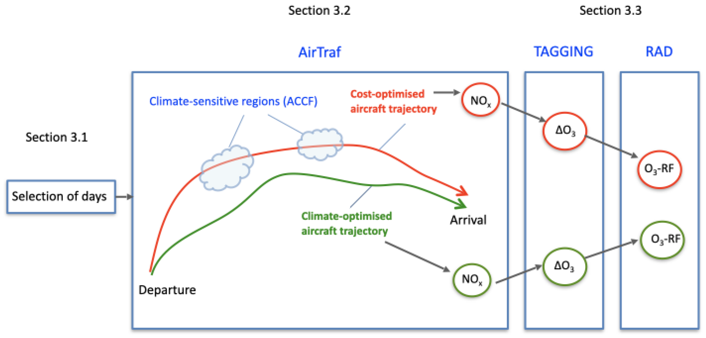
3. Numerical Experiments

The procedure evaluates the effectiveness of using the O${}_3$ aCCFs during air traffic optimisation for the actual reduction in climate impact (caused by aviation NO${}_x$ on O${}_3$) through performing numerical simulations with the aforementioned submodels. First, there is a one-year spin-up simulation in the period from August 2015 to August 2016. Following this, three steps are performed:

• The selection of days with a large variability of O${}_3$ aCCFs;
• The calculation of two aviation emission inventories for each selected day (step 1), i.e., for the cost-optimised and O${}_3$ aCCFs-optimised aircraft trajectories;
• The calculation of the contribution of NO${}_x$ emissions from step 2 to O${}_3$ mixing ratios and respective RF.

These steps are first discussed in Section 3.1, Section 3.2 and Section 3.3, respectively. We perform quasi-chemical-transport model (QCTM) simulations [50] with EMAC. These simulations are dedicated to ensure that the changes from the air traffic emissions do not feed back to the physical and dynamical processes in order to yield identical synoptic situations for the reference (background) and perturbed (additional NO${}_x$ emission) simulations.

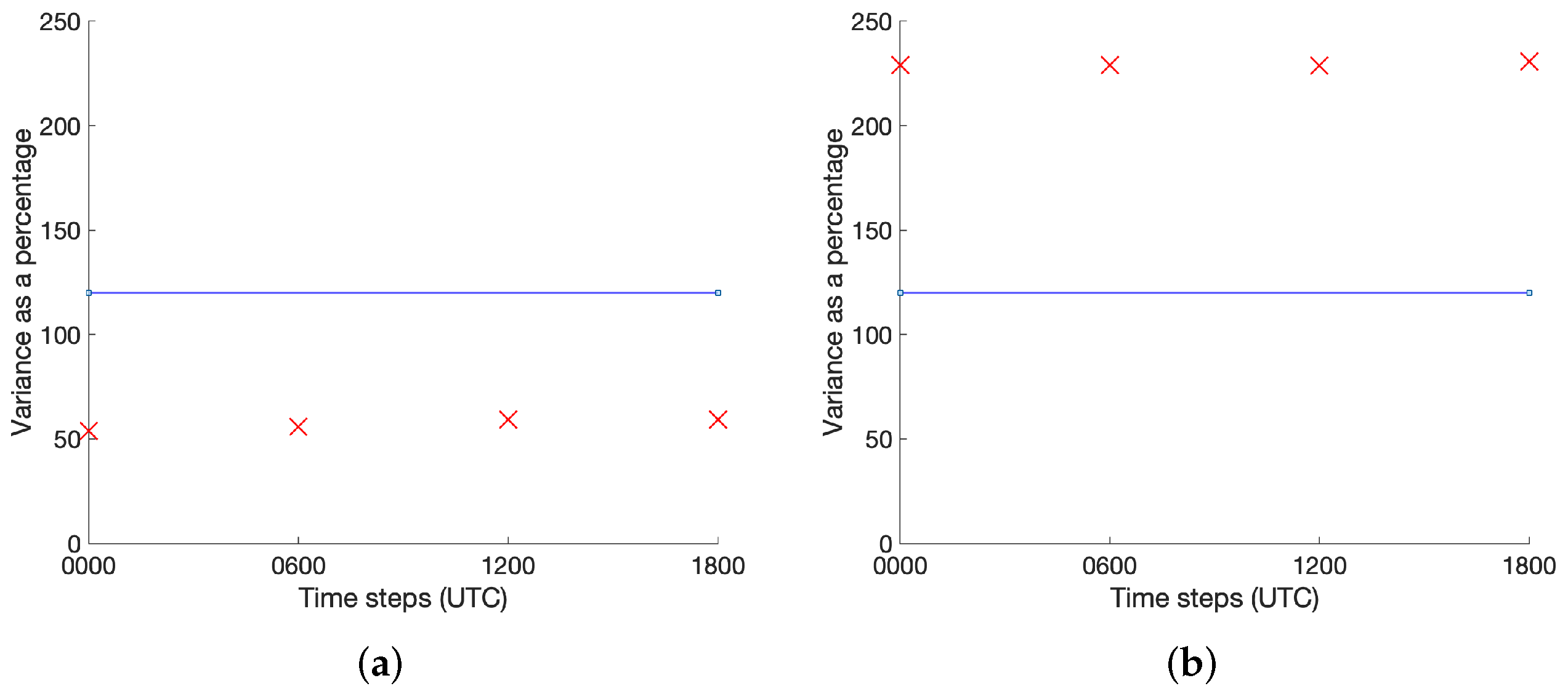
3.1. Procedure for Selection of Simulation Days

To test the validity of O${}_3$ aCCFs via trajectory optimisation, we choose specific days during which the variation of O${}_3$ aCCFs is large and allows a significant alteration of trajectories when optimising for NO${}_x$-O${}_3$ effects. In order to determine the variability of O${}_3$ aCCFs, a statistical approach is used. We analyse the variability of O${}_3$ aCCFs for the year 2016 based on European Centre for Medium-Range Weather Forecasts (ECMWF, https://www.ecmwf.int/, accessed on 20 October 2021) Re-Analysis Interim data [51] of temperature (T) and geopotential ($\Phi$) at a typical cruise flight pressure level of 250 hPa. For each day, $(T,\Phi )$ are recorded 4 times a day (6 h between them) and the O${}_3$ aCCFs (Equation (4)) is calculated offline for the longitude range (20° W to 35° E) and latitude range (25° N to 70° N) corresponding to the European airspace. We calculate the unbiased sample variance for each month (Equation (6)) and express it as a percentage of the monthly mean variance.

$${\sigma }^2=\frac{1}{N-1}\sum _{i=1}^N{\left(Y_i-\mu \right)}^2,$$

(6)

where $Y_i$ is the O${}_3$ aCCFs value for each time step with mean $\mu$ for $N=4\times k$ samples; k refers to the number of days in the specific month.

Here, we define a day with a large spatial variability of O${}_3$ aCCFs if the percentage variance exceeds 120%. These days occur about 6 times a month or 20% of the days in 2016, which is evident in Section 4.1. For example, small variability (Figure 5a) and large variability (Figure 5b) are compared for two days from March 2016. In Figure 5a, all the sample values (red) lie below the 120% line (blue), while in Figure 5b, they lie above the line. We are interested in large variability days for 2016.

The O${}_3$ aCCFs corresponding to those days are shown in Figure 6. The day characterised by large variability depicts a sharper contrast in the pattern. The lower and upper peak values have a larger spatial spread.

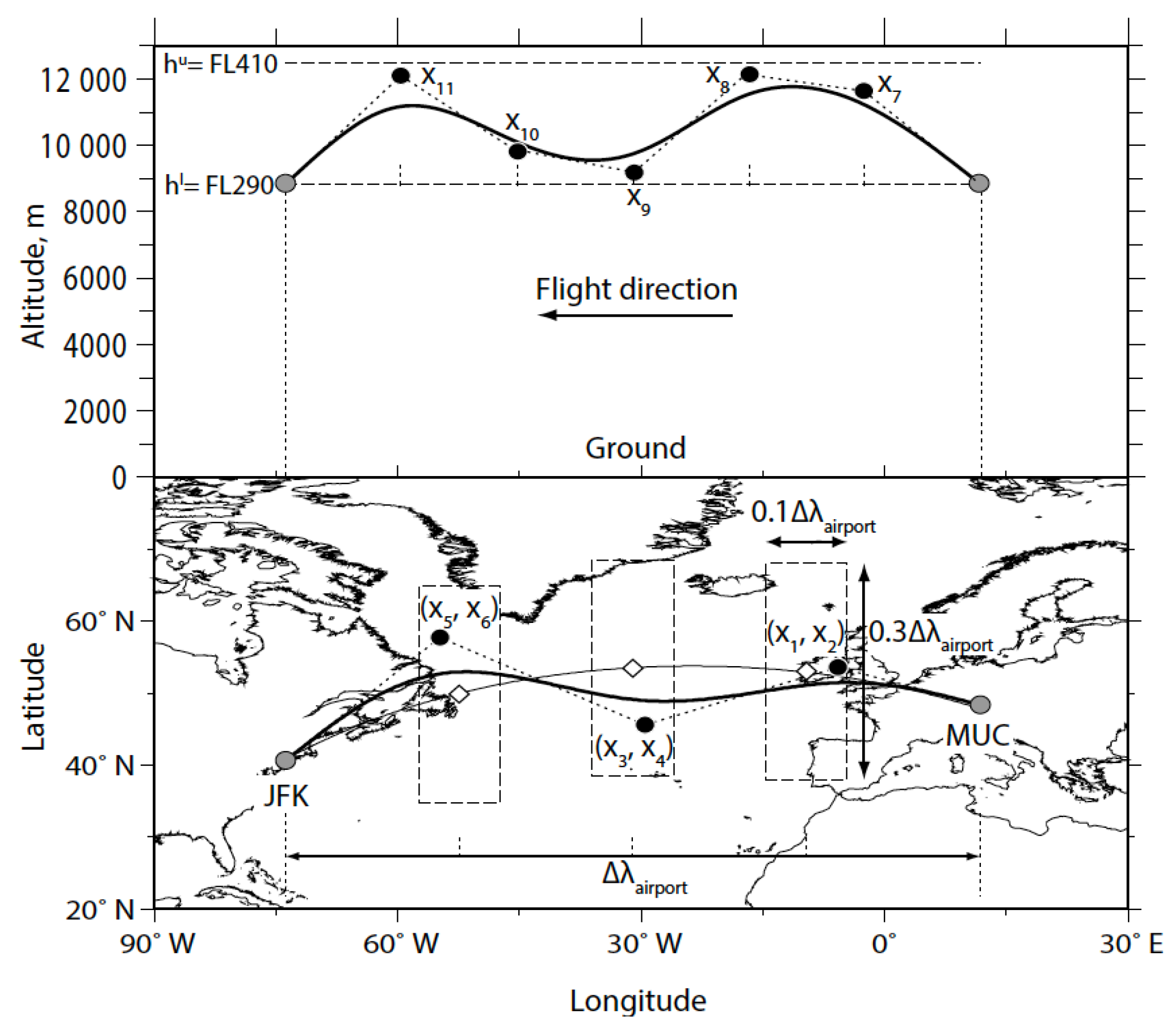
3.2. One-Day Air Traffic Simulation

For all synoptic situations, which are selected due to large spatial variability of O${}_3$ aCCFs (see also Section 2.2 and Section 4.1), a cost-optimised and climate-optimised (considering only O${}_3$ aCCFs) simulation is performed. To be specific, the cost-optimised simulation entails Simple Operating Cost (SOC), considering only flight time and fuel consumption [33], and is the baseline scenario. For each optimisation objective, the optimisation has been performed in two ways:

• Lateral re-routing: The flight corridor is fixed at an altitude of FL340 which corresponds to a typical cruise pressure level of 250 hPa by using constant vertical design variables (labelled $x_7$, …, $x_{11}$ in Figure 4). This way, the trajectory is optimised in terms of lateral re-routing called the horizontal analysis (HA).
• Vertical re-routing: The dashed boxes controlled by $x_1$, … $x_6$ (Figure 4) are fixed to the centre points of their respective rectangular domains. This way, the trajectory is laterally constrained and vertically optimised based on the depth of the cruise flight corridor called the vertical analysis (VA).

The idea behind this approach is to analyse, in detail, the climate impact (O${}_3$-RF) resulting from horizontal and vertical emission profiles after being subjected to the same synoptic situations. The above settings are used as inputs to ARMOGA to optimise trajectories with regard to SOC and climate impact of NO${}_x$-O${}_3$ effect in separate simulations (Figure 3). More details regarding the simulation and the flight plan are listed in

Table 2. One-day air traffic simulation setup.

Parameter	Optimisation Objective
	Cost-Optimised and Climate-Optimised (O${}_3$ aCCFs)
EMAC resolution	T42L31ECMWF (2.8 × 2.8°)
Time step of EMAC	12 min
Waypoints	101
Design variables	11 (6 locations and 5 altitudes)
Flight plan	85 European flights
Aircraft type	A330-301
Engine type	CF6-80E1A2, 2GE051 (with 1862M39 combustor)
Flight Mach number	0.82
Cruise flight altitude	Lateral re-routing	Vertical re-routing
	FL340 ≈ 10.4 km	[FL290, FL410] ≈ [8.8, 12.5] km

.

3.3. Four-Month Chemistry–Climate Simulation

Following the 1-day air traffic simulation, the NO${}_x$ emission data of the corresponding flights are recorded and input into a 4-month chemistry–climate simulation. The contribution of the AirTraf NO${}_x$ emissions to the tropospheric mixing ratios of NO${}_y$ (all active nitrogen species) and O${}_3$ is tracked over the simulation period using the TAGGING submodel (see Section 2.4). This duration of four months is sufficient to record the effect of NO${}_x$ emissions and has been proposed by other studies (e.g., [9,11,26,46]). The concentration and subsequent impact of emissions from the cost- and climate-optimised flights can be evaluated in detail. Finally, using the submodel RAD (see Section 2.5), the radiation budget is calculated (see also Figure 1). Note that the atmosphere also contains background emissions from other sources, such as aircraft, ships, road traffic, biomass and agricultural waste burning and other anthropogenic non-traffic emissions. Lastly, there are lightning emissions that are calculated online using the parameterisation described by Grewe et al. [52].

To summarise the simulation setup based on Section 3.1, Section 3.2 and Section 3.3, after selecting two representative winter and summer days characterised by large spatial variability of O${}_3$ aCCFs, there is a 1-day air traffic simulation on each of these days, which is followed by a chemistry–climate simulation that calculates mixing ratios of NO${}_y$ and O${}_3$ due to resulting aviation NO${}_x$ emissions over a 4-month period (

Table 3. Complete simulation setup.

Simulation Type	Optimisation Objective	Season	Variability of O${}_3$ aCCFs	Analysis	# Runs
1 day and 4 month	Cost and Climate	Summer and Winter	Large	HA and VA	16

). In the latter, the radiation budget is also calculated. The analysis is split into two components, namely HA and VA, in order to assess the horizontal and vertical pattern of O${}_3$ aCCFs and the climate impact from these different re-routing procedures. In total, we performed 16 simulations.

4. Results

First, the simulation days based on the procedure discussed in Section 3.1 are described in Section 4.1. A winter and summer day are chosen followed by the analysis of air traffic optimisation results for lateral and vertical re-routing in Section 4.2. In Section 4.3, the results from the chemistry–climate simulation are discussed for the two selected days. The influence of the synoptic situation on the transport of NO${}_x$ and the subsequent NO${}_y$ and O${}_3$ contributions is shown. Finally, the overall climate impact is derived and compared for all simulations in terms of O${}_3$-RF caused by optimised air traffic in Section 4.4.

4.1. Selection of Simulation Days

Following the procedure described in Section 3.1, the days with a large variability of the O${}_3$ aCCFs for the year 2016 are listed in

Table 4. Days with large variability of O${}_3$ aCCFs in the year 2016.

Month	Day of the Month
January	8–15, 30, 31
February	1–3
March	1–6, 22, 24
April	24–26, 28, 29
May	1–3, 12–14, 16, 18, 19
June	12–16
July	12, 13, 30, 31
August	1, 4, 5, 26–29
September	1–3, 5, 23, 27–30
October	1–3, 24
November	5, 6, 9
December	6, 7, 10, 11, 24, 26

. There is no specific pattern in how they are distributed. Here, we arbitrarily choose a winter day (1 February) and a summer day (1 August) from the list which have a percentage variance of ≈134 and ≈144%, respectively. Any day would be an equally good choice, but we choose days that are seasonally opposites because the synoptic situation on these days may be linked to the summer and winter weather patterns documented by Irvine et al. [53].

4.1.1. Synoptic Situation

The synoptic situation for the selected winter and summer day are shown in Figure 7a,b, which are comparable to the winter (W3) pattern and summer (S2) pattern of Irvine et al. [53], respectively. The selected winter day (Figure 7a) is characterised by the presence of high and low geopotential height anomalies [54], which indicate the presence of high-pressure (HP) and low-pressure (LP) systems, respectively. The HP system and high wind speeds (up to 60 m/s) that dominate the European airspace are expected to induce a south and downward transport of the bulk of the emitted species. On the other hand, the selected summer day (Figure 7b) is characterised by a zonal jet that is relatively slow (≈35 m/s) and with a smaller variation in the field. The synoptic situation on this day is expected to transport the bulk of the emitted species to higher latitudes (>50° N).

4.1.2. O${}_3$ aCCFs Pattern

The estimated impact of the NO${}_x$ emissions on O${}_3$ for the selected winter and summer days are shown in Figure 8b and Figure 9b, respectively. Because the O${}_3$ aCCFs are functions of temperature and geopotential (Equation (4)), the corresponding isolines are also depicted in Figure 8 and Figure 9. For the selected winter day, Figure 8b shows that lower (higher) latitudes are characterised by larger (smaller) values of the O${}_3$ aCCFs due to larger (smaller) values of the temperature and geopotential in these regions (see Rosanka et al. [25]). That is, for example, the Mediterranean region is characterised by large values of O${}_3$ aCCFs, while regions close to Iceland are characterised by low values of O${}_3$ aCCFs. There are slight similarities between the synoptic situation and the O${}_3$ aCCFs: the geopotential lines (Figure 8a) are similar in structure to the colour contours (Figure 8b). The O${}_3$ aCCFs show large values and hence strong warming effects in lower latitudes, where the bulk of the emitted species are expected to be transported (Figure 7a and their pathway indicated by the geopotential lines in Figure 8a).

For the selected summer day, Figure 9b similarly shows that lower (higher) latitudes are characterised by larger (smaller) values of the O${}_3$ aCCFs due to larger (smaller) values of the temperature and geopotential in these regions. There are slight similarities between the synoptic situation and the O${}_3$ aCCFs: the geopotential lines (Figure 9a) are similar in structure to the colour contours (Figure 9b). The temperature is higher (isolines in Figure 9b) compared to 1 February (isolines in Figure 8b) with a very different geopotential field. Consequently, the O${}_3$ contribution from the NO${}_x$ emissions estimated by the O${}_3$ aCCFs is also larger. However, the synoptic situation on the selected summer day (Figure 7b and the pathway of the emissions as indicated by the geopotential lines in Figure 9a) is expected to transport emitted NO${}_x$ to higher latitudes (>40° N). Yet, O${}_3$ effects are predicted to be stronger at the lower latitudes by the O${}_3$ aCCFs, owing to the strong dependence on temperature and geopotential in Equation (4), which is a limitation (Figure 9b).

The vertical distribution of the O${}_3$ aCCFs for the selected days can be visualised by plotting its meridional mean in the European area as shown in Figure 10. The pressure levels [315, 180] hPa correspond roughly to the flight corridor within [FL290, FL410]. Most of the climate sensitive regions lie at higher altitudes.

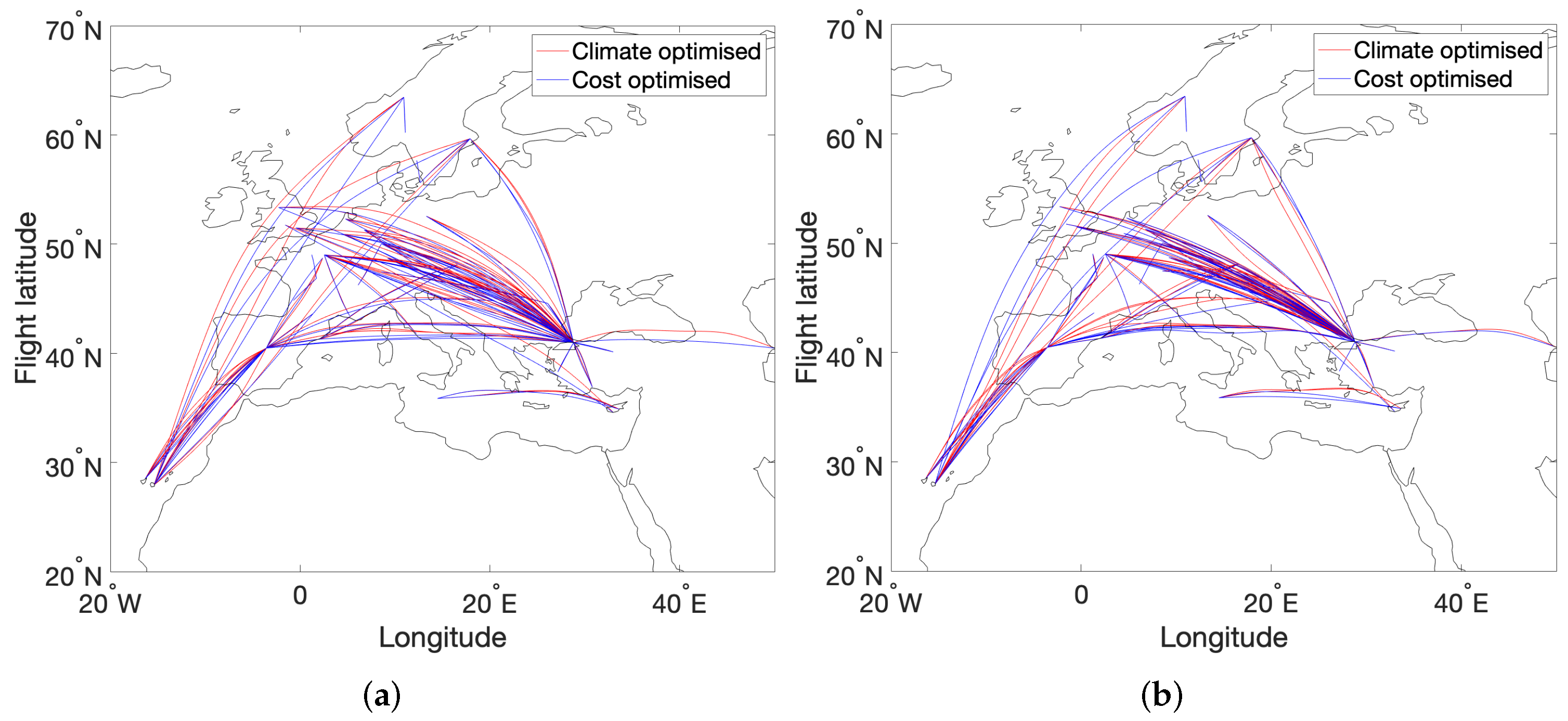
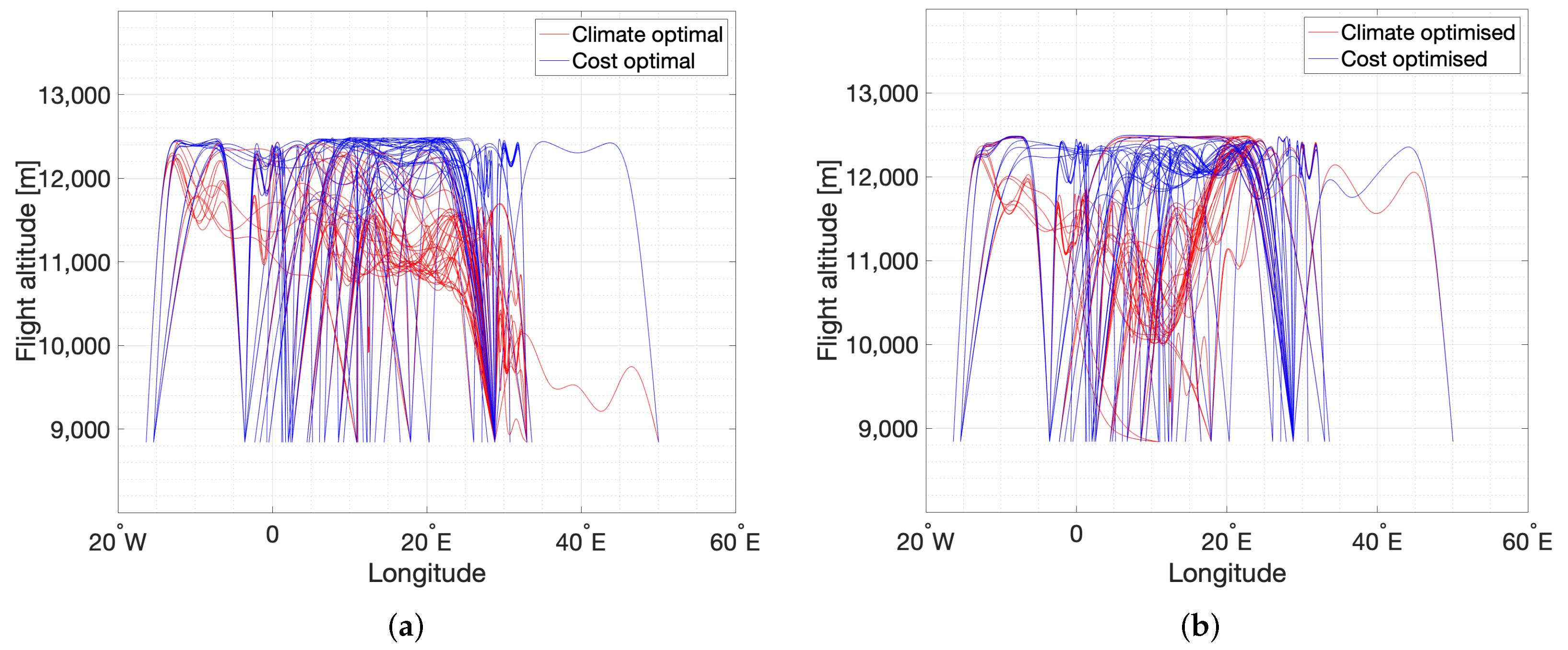
4.2. Optimised Air Traffic

In this section, we first look into the results for the 1-day air traffic simulation for the lateral re-routing on the selected winter and summer days. There are 85 flights in the flight plan and the flight altitude is fixed at FL340, corresponding to a typical cruise pressure level of 250 hPa (Table 2). Therefore, we only see lateral changes in the routing for cost-optimised (blue) and climate-optimised (red) flights on the chosen winter day and summer day (Figure 11), respectively. It is indeed artificial to fix a cruise flight altitude, but this is done to analyse lateral shifts in trajectories for the two routing objectives. Because the flight trajectories are essentially curves and hence functions, we can compute the relative change of climate-optimised flights with respect to cost-optimised flights in ${\mathbb{R}}^2$ (because cruise altitude is fixed). The ${\mathcal{L}}^2$ norm [55] is used to compute this for all the flight trajectories. The maximum deviation between the climate- and cost-optimised flight trajectories is found to be ≈11.5 and ≈6.5% on the selected winter and summer days, respectively. The mean lateral deviation for all the flight trajectories was found to be ≈1% on both the selected days. In most cases, climate-optimised flights are shifted to the North, where the O${}_3$ impact is predicted to be lower (Figure 8 and Figure 9b).

In the case of vertical re-routing, the lateral changes for cost- and climate-optimised flights are fixed. Figure 12a,b illustrate the vertical changes of climate-optimised (red) and cost-optimised (blue) flights on the selected winter and summer days, respectively. The vertical shift in trajectories is calculated using the same procedure, while laterally, flight trajectories remain unchanged. The maximum deviation between the climate-optimised and cost-optimised flight trajectories is found to be ≈22 and ≈26% on the selected winter and summer days, respectively. The mean vertical deviation for all the flight trajectories is found to be ≈7.5 and ≈5.5% on the selected winter and summer days, respectively. Therefore, in the case of vertical re-routing, the differences between flight trajectories are considerably larger than in lateral re-routing.

For the vertically re-routed cost-optimised flights, there are no significant quantitative differences in flight altitude for two selected days. This is because the total cost mainly depends on the flight time and fuel consumption. To reduce the flight time, aircraft fly along a jet stream, and to reduce the fuel cost, aircraft stay at higher altitudes. As the optimiser considers both effects, it found that there is a bigger advantage to flying higher for the two selected days. This also implies that the synoptic situation that is relevant for the contribution of O${}_3$ from the NO${}_x$ emissions does not play a major role in the cost optimisation. On the contrary, for the O${}_3$ aCCFs-optimised flights, large differences are seen in the two days which indicates that the situation is more complex as the NO${}_x$-O${}_3$ effects depend on various factors as discussed in Section 1. The climate-sensitive regions lie more at higher altitudes (Figure 10), and the O${}_3$ aCCFs-optimised flights avoid the most sensitive regions by flying lower. On the selected winter day, there is a tendency for many flights to drift to lower altitudes at eastward longitudes (Figure 12a). On the selected summer day, many flights seem to prefer flying even lower than in the winter at ≈10,000 m (Figure 12b); however, a few flights also move to slightly higher altitudes (around 12,000 m, i.e., corresponding to ≈190 hPa).

Table 5. Fuel consumption, NO${}_x$ emissions, mean EINO${}_x$ and total flight time from laterally and vertically re-routed flights.

Optimisation Objective	Selected Day	Fuel Consumption [$\times {10}^3$ kg]		NO${}_{\mathit{x}}$ Emission [$\times {10}^6$ g (NO${}_{\mathit{x}}$)]		EINO${}_{\mathit{x}}$ [g (NO${}_{\mathit{x}}$)/kg (Fuel)]		Flight Time (Hour)
		Lateral	Vertical	Lateral	Vertical	Lateral	Vertical	Lateral	Vertical
Cost-optimised	Summer	815	742	10.3	8.92	12.6	12	150	152
	Winter	813	747	9.18	7.52	11.3	10.1	153	157
Climate-optimised	Summer	816	771	10.2	9.23	12.5	12	151	152
	Winter	815	777	9.15	8.15	11.2	10.5	154	156

summarises the fuel consumption, the amount of NO${}_x$ emitted, the mean emission index of NO${}_x$ (EINO${}_x$) and the total flight time for each case that is considered. In all cases of lateral re-routing, the amount of fuel consumption and NO${}_x$ is almost the same for the cost-optimised and climate-optimised flights. For vertical re-routing, in both the winter and summer, climate-optimised flights consume ≈4% more fuel. In winter, they emit ≈8% more NO${}_x$ than cost-optimised flights, and in the summer, ≈3.5% more NO${}_x$ than cost-optimised flights. Therefore, for vertical re-routing, we have higher overall emissions for the climate-optimised case, which is consistent with results from Yin et al. [27]. The amount of NO${}_x$ reported in Table 5 is a product of fuel burn and EINO${}_x$. The climate-optimised trajectories favour lower flight altitudes, which increases the fuel consumption and EINO${}_x$ driven by a higher thrust setting for a constant flight Mach number. Therefore, the total NO${}_x$ of climate-optimised flights increases. However, the climate impact of NO${}_x$ depends not only on the quantity of NO${}_x$ emissions but also on the location where NO${}_x$ is emitted. At lower altitudes, the residence time of NO${}_x$ is shorter (e.g., [56,57]), hence leading to less O${}_3$ formation and therefore reducing the NO${}_x$-O${}_3$ climate impact, which is evident in Section 4.4 and consistent with other studies (e.g., [57]). The mean deviation in the total flight time between climate- and cost-optimised trajectories is less than 0.5%. Hence, relative changes in flight time are found to be negligible compared to fuel consumption.

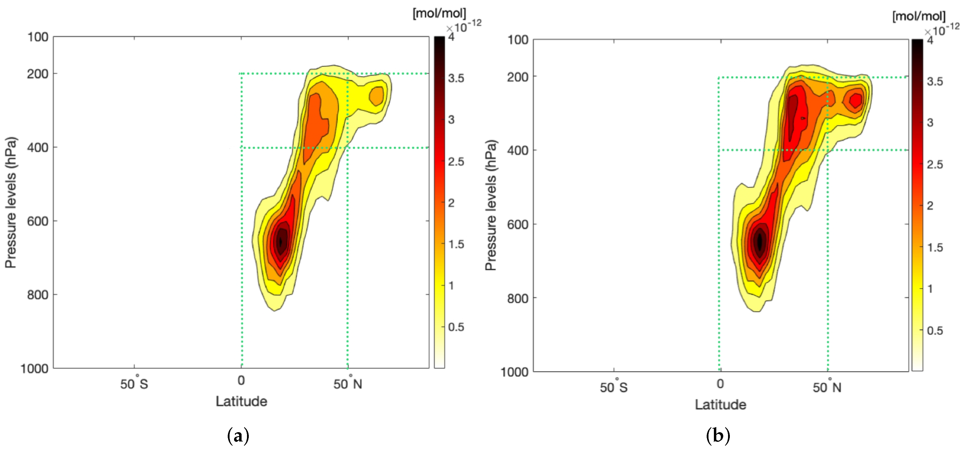
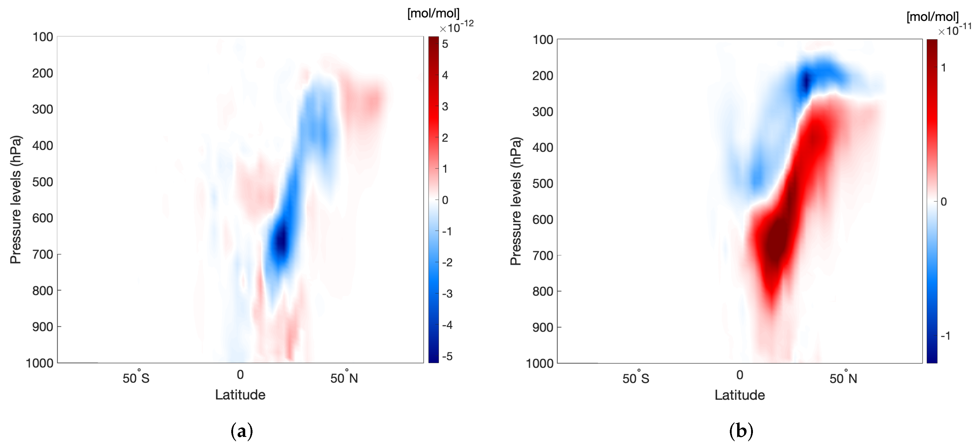
4.3. Chemistry–Climate Results

The TAGGING submodel tracks the contribution of the NO${}_x$ emissions from the optimised air traffic to the tropospheric NO${}_y$ and O${}_3$ mixing ratio from the time at which the emissions are released until the four-month simulation period is complete. These fields are denoted as NO${}_y$atf and O${}_3$atf, respectively. Since the synoptic situations on the two selected days are different, we separate the results for the two days.

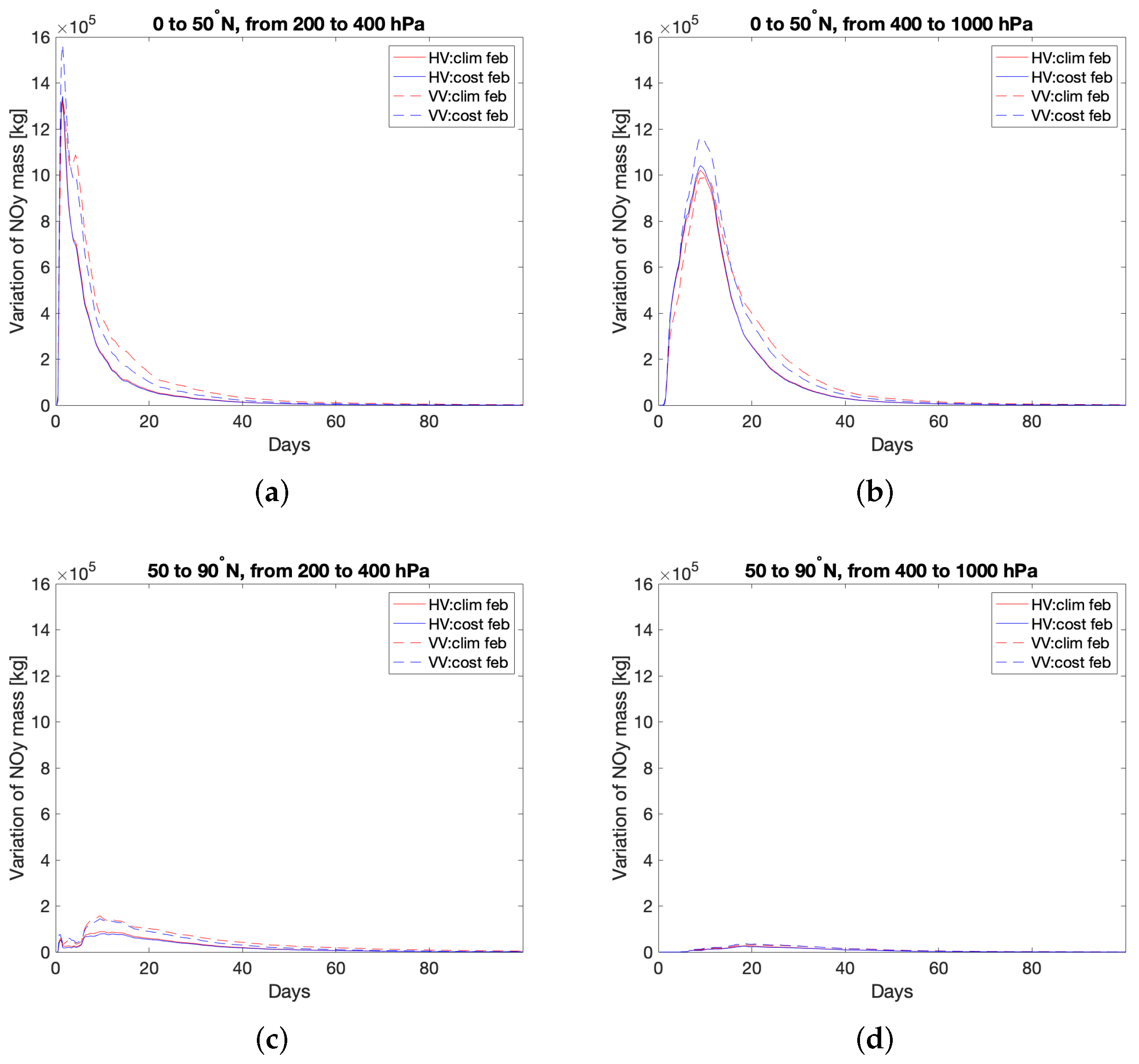
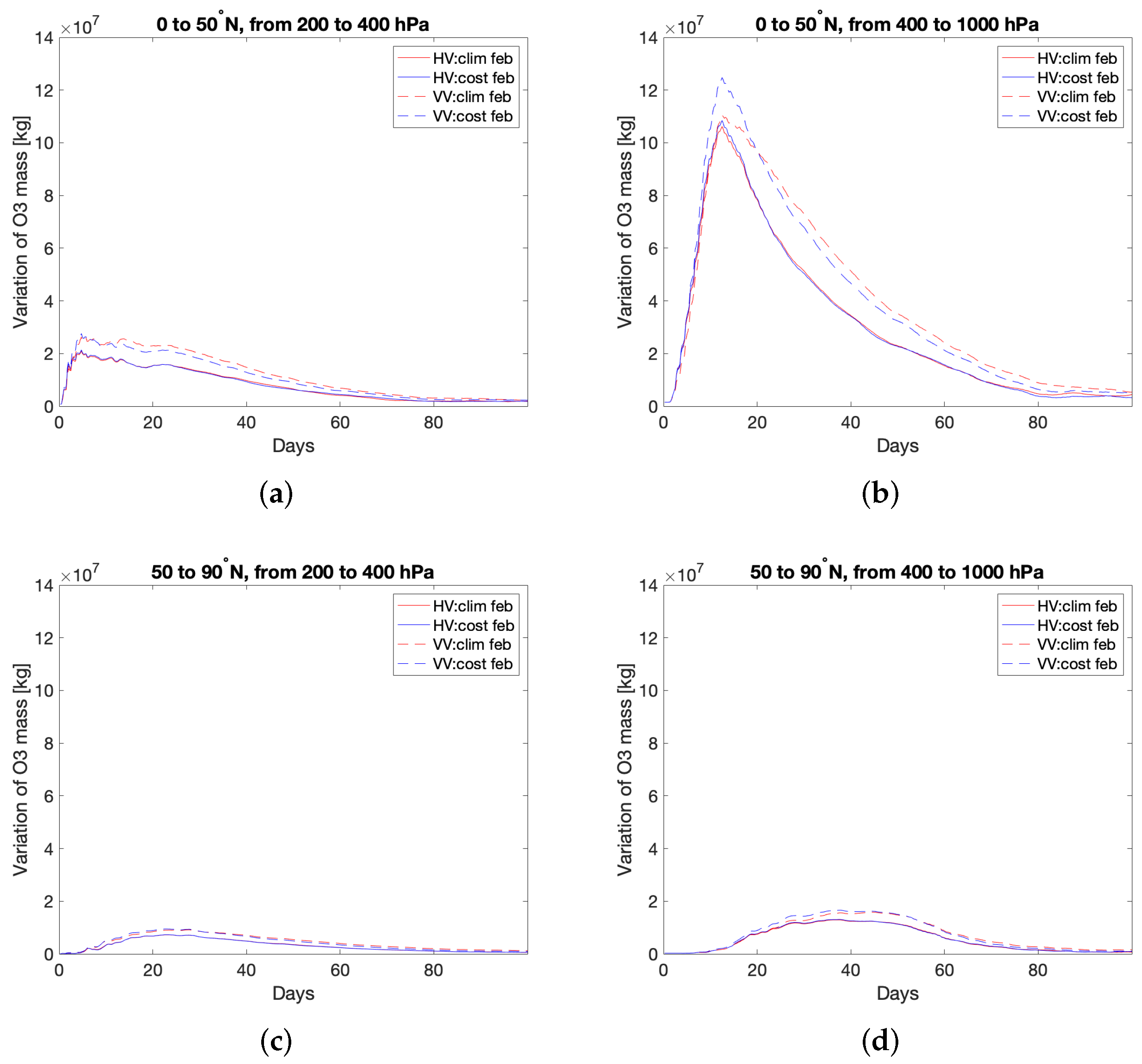
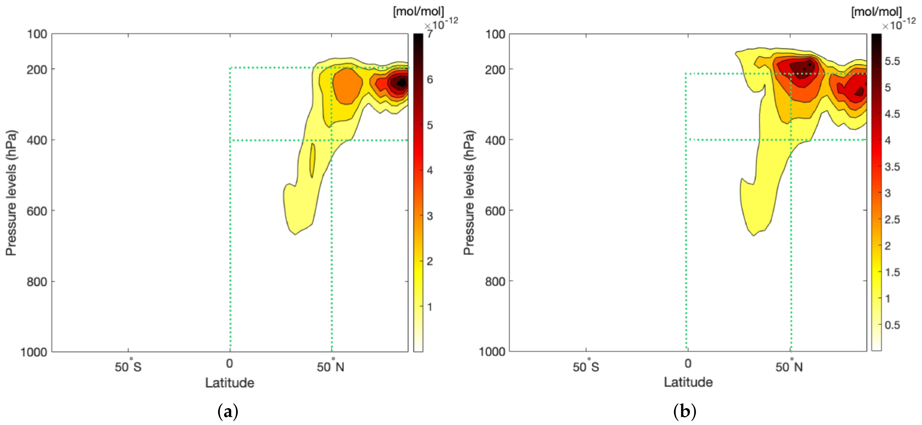
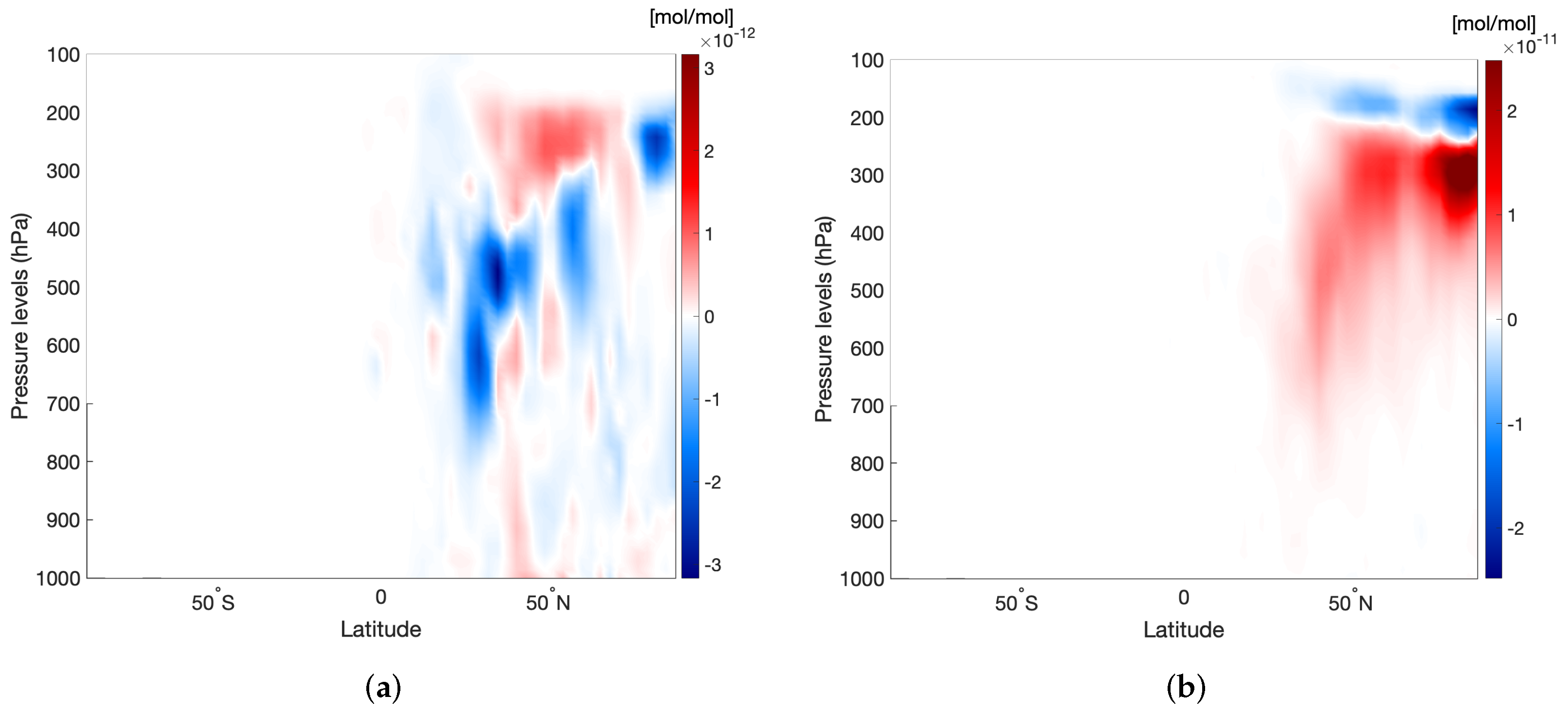
4.3.1. Selected Winter Day

Figure 13a,b illustrate the patterns for the zonal mean of NO${}_y$atf, taken along the longitudes, one week since the emissions are released from laterally re-routed and vertically re-routed climate-optimised flights, respectively. The patterns look similar in both cases, with peak values located at lower altitudes (≈600 to 700 hPa) and lower latitudes (≈20° N), approaching towards the equator. However, in the case of vertical re-routing, large values are also spread across the vertical pressure levels (≈200 to 400 hPa). Therefore, the location of the bulk of the emissions are at lower latitudes and altitudes, which is to be expected from the synoptic situation (Figure 7 and Figure 8a).

The difference of the zonal mean O${}_3$atf mixing ratios between climate- and cost-optimised flights on the selected winter day is depicted in Figure 14. In the case of lateral re-routing (Figure 14a), the O${}_3$atf mixing ratio is larger for cost-optimised flights. In winter, there is less photochemical activity in general; climate-optimised flights are using predominantly higher latitudes, whereas cost-optimised flights use predominantly lower latitudes. As the photochemical activity is more prominent at lower latitudes, the O${}_3$atf mixing ratio decreases considerably for climate-optimised flights. In the case of vertical re-routing (Figure 14b), climate-optimised flights use preferably lower flight altitudes (Figure 12a), where higher production of O${}_3$ occurs. This matches with the results from the air traffic optimisation (Figure 12a), where most climate-optimised flights took place at low altitudes. The region of the O${}_3$atf production is crucial for the resulting RF, which is shown in Section 4.4.

The green dotted boxes in Figure 13 indicate four regions of interest that are further investigated. Figure 15 shows the time series of the mass of NO${}_y$atf in these regions for all the climate- and cost-optimised simulations on the selected winter day. For the conversion of the NO${}_y$atf from mixing ratio to mass, the molar mass of nitrogen (N) (14 kg/kmol) is used throughout this study. The regions where most of the NO${}_y$atf is present are (a) and (b) in Figure 15. In the first few days of the simulation, most of the NO${}_y$atf is present in the former region (i.e., at cruise-level altitudes) and thereafter the bulk is transported to the latter region (i.e., lower altitudes). Additionally, the deviation in the time series of the NO${}_y$atf between climate-optimised and cost-optimised simulations is larger for the vertical re-routing than for the lateral re-routing. Finally, regions (c) and (d) do not show significant activity.

Similarly, Figure 16 shows the time series of the mass of the O${}_3$atf in these regions for the climate- and cost-optimised simulations on the selected winter day. In the first five days of the simulation, the O${}_3$atf mass peaks in region (a), but thereafter, the bulk of the O${}_3$atf rises rapidly in region (b), i.e., at lower altitudes corresponding to 400 to 1000 hPa. On the contrary, the other two regions, which correspond to higher latitudes, are characterised by very low amounts of O${}_3$atf. Moreover, more O${}_3$atf is produced from cost-optimised simulations compared to climate-optimised simulations, which is expected to lead to higher O${}_3$-RF (Section 4.4).

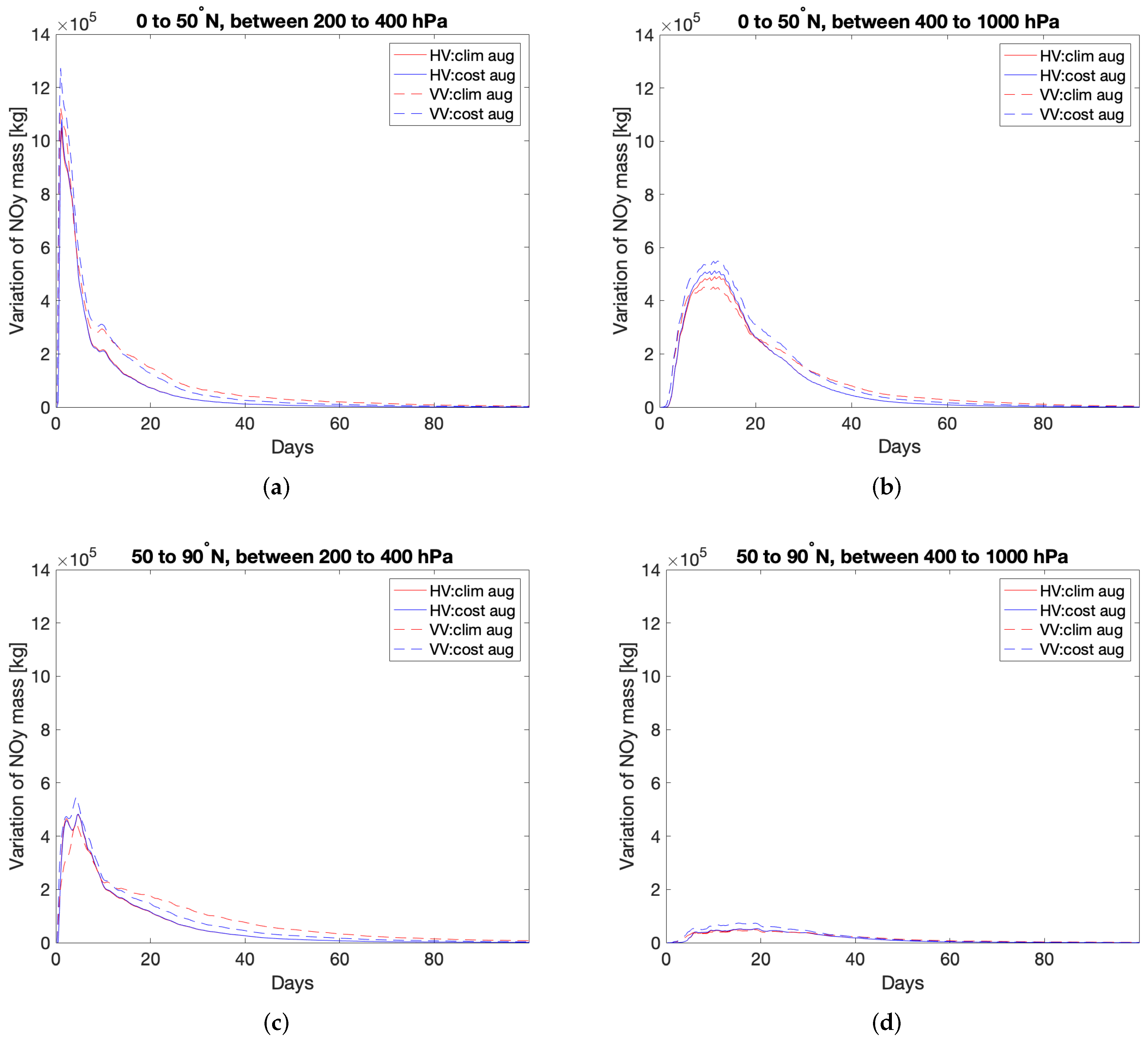
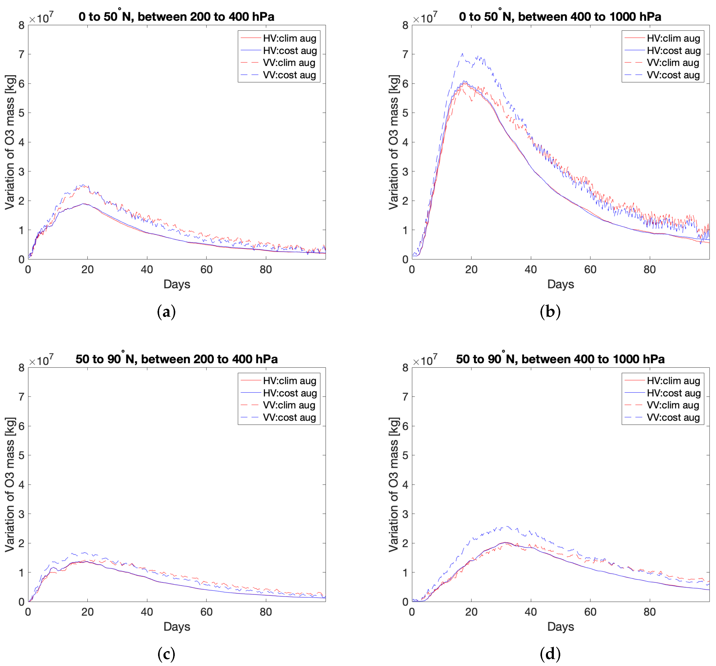
4.3.2. Selected Summer Day

Figure 17a,b illustrate the zonal mean NO${}_y$atf, one week since the emissions are released from laterally re-routed and vertically re-routed climate-optimised flights, respectively. These patterns are distinct from the winter case (Figure 13). In the case of lateral re-routing (Figure 17a), there is a localised peak at the cruise level (≈250 hPa) and towards the North pole (≈80° N). In the case of vertical re-routing (Figure 17b), there are two distinct peaks, also concentrated at cruise altitudes (≈200 and 300 hPa), either upper mid-latitudes (≈50° N) or close to the North pole (≈80° N). In both cases of the selected summer day, the bulk of the emissions can be found at high altitudes and towards higher latitudes (>50° N), which is to be expected from the synoptic situation (Figure 7b and Figure 9a).

The difference of the zonal mean O${}_3$atf mixing ratios between climate- and cost-optimised flights on the selected summer day is depicted in Figure 18. There is a strong contrast to the winter case (Figure 14). In summer, there is a lot more photochemical activity than in the winter and hence the difference in O${}_3$atf production does not have a single localised peak. This is especially clear for lateral re-routing (Figure 18a), where the O${}_3$atf mixing ratio is seen to be mainly larger for cost-optimised flights. In the case of vertical re-routing (Figure 18b), most climate-optimised flights take place at lower altitudes (Figure 12b), where the emissions are subject to higher O${}_3$ production. This results in higher O${}_3$atf mixing ratios in general and larger for climate-optimised flights. This matches with the results from the air traffic optimisation (Figure 12b), where most climate-optimised flights took place at lower altitudes compared to cost-optimised flights. The region of the O${}_3$atf production is crucial for the resulting RF, which is shown in Section 4.4.

The green dotted boxes in Figure 17 indicate four regions of interest that are further investigated. Figure 19 shows the time series of the mass of the NO${}_y$atf in these regions for all the climate- and cost-optimised simulations on the selected summer day. The regions where most of the NO${}_y$atf is present are (a), (b) and (c) in Figure 19. In the first two days of the simulation, most of the NO${}_y$atf is present in region (a) (i.e., at cruise-level altitudes). A part of it is transported to region (c) (i.e., higher latitudes but at cruise level), and after a few days, the NO${}_y$atf is transported to region (b) (i.e., lower altitudes). After one week, region (b) is seen to have the highest amount of NO${}_y$atf. Finally, the deviation in the time series of the NO${}_y$atf between climate-optimised and cost-optimised simulations is larger for vertical re-routing than for lateral re-routing.

Similarly, Figure 20 shows the time series of the O${}_3$atf mass in these regions for all the climate- and cost-optimised simulations on the selected summer day. In all four regions of Figure 20, the O${}_3$atf mass is seen to rise with the bulk of the O${}_3$atf rising rapidly in region (b) after one week, i.e., at lower altitudes corresponding to 400 to 1000 hPa but within 0 to 50° N. Moreover, more O${}_3$atf is produced from cost-optimised simulations compared to climate-optimised simulations, which is expected to lead to higher O${}_3$-RF (Section 4.4).

4.4. Radiative Forcing

The mean O${}_3$-RF (stratospheric-adjusted) from the AirTraf NO${}_x$ over the 4-month chemistry–climate simulation period for all the simulations are listed in

Table 6. Comparison of mean RF of O${}_3$ from optimised air traffic for emissions as given in Table 5.

Air Traffic Optimised on	Type of Analysis	Mean RF of O${}_3$ [$\mathsf{\mu }$W/m${}^2$]		% Reduction
		Cost-Optimised	Climate-Optimised
Winter day	Horizontal	84.1	83.7	0.5
	Vertical	96.9	94.6	2.4
Summer day	Horizontal	96.4	95.6	0.8
	Vertical	148	119	20

. First and foremost, it can be seen that the O${}_3$-RF is larger for cost-optimised simulations compared to climate-optimised simulations. This corroborates the findings of Yin et al. [27]. The summer flights lead to larger climate impact than the winter flights in terms of O${}_3$-RF, because of greater photochemical activity in the summer, indicating stronger NO${}_x$-O${}_3$ effects in the summer, which supports previous studies (e.g., Gauss et al. [58] and Frömming et al. [9]).

For lateral optimisation, i.e., for a fixed cruise level of 250 hPa, the O${}_3$-RF is lower compared to vertical optimisation despite larger fuel consumption and NO${}_x$ emitted compared to those for the vertical re-routing (Table 5). Looking back at the mixing ratio of NO${}_y$ for lateral re-routing (Figure 13a and Figure 17a), it can be seen that the peak values are less dispersed compared to vertical re-routing. For both of the selected days (Figure 13b and Figure 17b), the peaks are separated and are at significantly different pressure levels (≈650 and ≈300 hPa) in the winter and at different latitudinal locations (≈55° N and ≈85° N) in the summer. Additionally, the NO${}_y$ field is more dispersed in the vertical re-routing case, which means that it is less influenced by atmospheric processes, such as wash-out and dry deposition, compared to the lateral re-routing case. Lastly, the time series of the O${}_3$ mass in Figure 16 and Figure 20 indicate lower values for lateral re-routing compared to vertical re-routing. As a result, the O${}_3$-RF from vertical re-routing is larger compared to that from lateral re-routing.

Thus far, no studies are available that have analysed the mean O${}_3$-RF based on aviation NO${}_x$ emissions occurring on a single day. Yin et al. [27] reported a mean O${}_3$-RF of ≈13 mW/m${}^2$, but this involved an air traffic simulation for the same flight plan as used in this study, repeated every day for a period of 90 days (as opposed to a single day in the present study). Because radiative calculations are non-linear, it is not possible to make a direct and accurate comparison between these two studies. However, taking a rough estimate, the mean RF that can be attributed to a single day is $\frac{13}{90}$ mW/m${}^2\approx$ 140 $\mathsf{\mu }$W/m${}^2$, which has the same order of magnitude as the values listed in Table 6. Other studies, such as Lee et al. [22] and Lee et al. [2], provide the best estimates of a global aviation RF of 26.3 and 36.0 mW/m${}^2$, respectively, from short-term O${}_3$ production based on several aviation NO${}_x$ emission inventories.

Finally, the difference between climate- and cost-optimised flights in mean O${}_3$-RF over the period of four months is larger for vertically re-routed flights, which can be attributed to the larger difference in O${}_3$ production compared to that from laterally re-routed flights (Figure 16 and Figure 20). The largest reduction of 20% occurred for vertically re-routed flights on the selected summer day, while the smallest reduction of 0.5% occurred for laterally re-routed flights on the selected winter day (Table 6).

5. Discussions and Conclusions

The possibility of reducing aviation’s overall climate impact requires us to take into account various non-CO${}_2$ effects such as H${}_2$O, contrails, aerosols and NO${}_x$ effects on O${}_3$ and CH${}_4$. This study looked specifically into short-term NO${}_x$ effects on O${}_3$ production, a phenomenon that is governed by several competing factors, such as emission location and time, synoptic situation, transport pathways and photochemical activity. The prototype O${}_3$ aCCFs were introduced as a tool to facilitate the prediction of O${}_3$ CCFs by means of instantaneous weather data (temperature and geopotential) without the need for the computationally expensive procedure of recalculating CCFs. However, this comes at a cost of larger uncertainties and lower accuracy, which necessitates a study to test its validity. Hence, the hypothesis was that O${}_3$ aCCFs can mitigate short-term aviation NO${}_x$-O${}_3$ effects compared to cost-optimised flights for days characterised by a large spatial variability of O${}_3$ aCCFs.

It was shown that under large weather variability (Section 4.1), O${}_3$ aCCFs were able to generate more climate-friendly flights than the cost-optimised flights for the two specific weather patterns, thereby complying with findings by Yin et al. [27]. The impact of the weather situation on the selected winter and summer days and the subsequent transport pathways proved to be very crucial in the climate impact of flights as was discussed in earlier studies (e.g., [9,12,25]). While looking into detailed 1-day air traffic optimisation, it was found that, on average, for climate-optimised flights, there was a much larger deviation in vertical re-routing compared to lateral re-routing. Although laterally re-routed flights consumed more fuel and emitted more NO${}_x$ than vertically re-routed flights, the climate impact was still lower. This can be attributed to the location and spread of NO${}_x$ emissions and possibly the choice of cruise level. It would help extending the analysis to other cruise levels to test the sensitivity of O${}_3$ production and the subsequent RF, as the corresponding findings can also be compared with other studies (e.g., [57,58,59]). For vertically re-routed flights, the difference in the O${}_3$-RF between climate- and cost-optimised flights (and hence climate mitigation potential) was found to be larger than for laterally re-routed flights. Because the flight altitude was variable in this case of vertical re-routing, the NO${}_x$ emissions were subjected to different chemical regimes. Additionally, the emissions were also driven by the transport pathway, causing a larger difference in O${}_3$ production and, hence, RF. The NO${}_x$-O${}_3$ effects were found to be stronger in the summer period than in winter, which also agrees with previous studies (e.g., [25,60]). Although those findings in general might apply to other seasons, future studies could check if there are any special features due to various photochemical regimes for NO${}_x$-O${}_3$ effects. Additionally, NO${}_x$ emitted at lower altitudes has a shorter residence time (e.g., [56,57]), resulting in a further reduction in climate impact for vertically re-routed flights for the selected summer day.

For the RF calculation for an O${}_3$ perturbation, a more advanced radiation flux change is required than instantaneous RF at the tropopause, because it is not a reliable predictor for expected resulting temperature change [61]. On the other hand, the simulation set-up employing pulse emissions is not well suited to derive stratospheric-adjusted RFs or effective RFs. To overcome this discrepancy, Grewe et al. [11] and Frömming et al. [9] applied a post-processing to their instantaneous RF values, converting them into stratospheric-adjusted RFs on the basis of a range of pre-calculated scenarios. However, a revision for this procedure might be necessary [14]. Therefore, here, we decided to consistently apply the adjusted RF calculation (this value covers only a part of the stratospheric temperature adjustment, as a full adjustment could not be covered due to a simulation length of just four months) for the cost- and O${}_3$ aCCFs-optimised air traffic, using the RAD submodel (Section 4.4).

In the present study, we looked at flight optimisation in the European airspace, but it might help extending the analysis to the North Atlantic region where there is more freedom for routing to change: longer distances allowing detours and identifiable weather patterns [53]. Finally, Frömming et al. [9] took into account the influence of the weather on the total NO${}_x$ CCFs. This total effect includes not just the short-term increase in O${}_3$ but also a long-term decrease in CH${}_4$ and a CH${}_4$-induced decrease in O${}_3$ (PMO and stratospheric water vapour decrease). In order to take this total effect into account for arbitrary situations using aCCFs, the current CH${}_4$ aCCFs need to be carefully evaluated [14]. Note also that there was a strong connection between the weather situation and O${}_3$ CCFs as shown by Frömming et al. [9], but the O${}_3$ aCCFs do not capture all features equally well (Figure 8b and Figure 9). Hence, while the aCCFs in general are useful in calculating real-time flight trajectories for the sake of climate impact mitigation, looking at ways of improving them will lead to much needed improved predictions of climate impact from non-CO${}_2$ effects of aviation, which are highly needed. We intend to do this by extending the CCFs and the consequent aCCFs to more regions, e.g., Africa, Australasia, Eurasia, North and South America, and to use more powerful statistical techniques. The use of the concept in daily operations seems to be feasible; however, it requires several steps to make it operational. Roadmaps have been outlined in Figure 4 of Grewe et al. [62] and Figure 9 of Matthes et al. [63] that comprise an investigation of uncertainties and robustness of such aCCFs concepts (see also Matthes et al. [64]), impacts on air traffic densities and hot spots and the exploration of economic measures. As a result, climate-optimised flight planning could be practically feasible.

References

1. IPCC. Climate Change 2021: The Physical Science Basis. Contribution of Working Group I to the Sixth Assessment Report of the Intergovernmental Panel on Climate Change; Cambridge University Press: Cambridge, UK, 2021. [Google Scholar]
2. Lee, D.; Fahey, D.; Skowron, A.; Allen, M.; Burkhardt, U.; Chen, Q.; Doherty, S.; Freeman, S.; Forster, P.; Fuglestvedt, J.; et al. The contribution of global aviation to anthropogenic climate forcing for 2000 to 2018. Atmos. Environ. 2021, 244, 117834. [Google Scholar] [CrossRef] [PubMed]
3. Grewe, V.; Rao, A.G.; Grönstedt, T.; Xisto, C.; Linke, F.; Melkert, J.; Middel, J.; Ohlenforst, B.; Blakey, S.; Christie, S.; et al. Evaluating the climate impact of aviation emission scenarios towards the Paris agreement including COVID-19 effects. Nat. Commun. 2021, 12, 3841. [Google Scholar] [CrossRef] [PubMed]
4. ICAO. Annual Report. In The World of Air Transport in 2018. 2018. Available online: https://www.icao.int/annual-report-2018/Pages/the-world-of-air-transport-in-2018.aspx (accessed on 20 October 2021).
5. Airbus. Global Market Forecast 2018–2037. In Global Networks, Global Citizens. 2018. Available online: https://www.airbus.com/sites/g/files/jlcbta136/files/2021-07/Presentation-Eric-Schulz-GMF-2018.pdf (accessed on 20 October 2021).
6. Boeing. Commercial Market Outlook 2019–2038. 2019. Available online: https://s4cd98e6181776fd7.jimcontent.com/download/version/1597359309/module/8027287461/name/cmo-sept-2019-report-final.pdf (accessed on 20 October 2021).
7. Grewe, V.; Stenke, A. AirClim: An efficient tool for climate evaluation of aircraft technology. Atmos. Chem. Phys. 2008, 8, 4621–4639. [Google Scholar] [CrossRef] [Green Version]
8. Köhler, M.O.; Rädel, G.; Dessens, O.; Shine, K.P.; Rogers, H.L.; Wild, O.; Pyle, J.A. Impact of perturbations to nitrogen oxide emissions from global aviation. J. Geophys. Res. 2008, 113. [Google Scholar] [CrossRef] [Green Version]
9. Frömming, C.; Grewe, V.; Brinkop, S.; Jöckel, P.; Haslerud, A.S.; Rosanka, S.; van Manen, J.; Matthes, S. Influence of weather situation on non-CO2 aviation climate effects: The REACT4C climate change functions. Atmos. Chem. Phys. 2021, 21, 9151–9172. [Google Scholar] [CrossRef]
10. Matthes, S. REACT4C—Climate Optimised Flight Planning. In Innovation for Sustainable Aviation in a Global Environment; IOS Press: Amsterdam, The Netherlands, 2012; pp. 122–128. [Google Scholar] [CrossRef]
11. Grewe, V.; Frömming, C.; Matthes, S.; Brinkop, S.; Ponater, M.; Dietmüller, S.; Jöckel, P.; Garny, H.; Tsati, E.; Dahlmann, K.; et al. Aircraft routing with minimal climate impact: The REACT4C climate cost function modelling approach (V1.0). Geosci. Model Dev. 2014, 7, 175–201. [Google Scholar] [CrossRef] [Green Version]
12. Grewe, V.; Champougny, T.; Matthes, S.; Frömming, C.; Brinkop, S.; Søvde, O.; Irvine, E.; Halscheidt, L. Reduction of the air traffic’s contribution to climate change: A REACT4C case study. Atmos. Environ. 2014, 94, 616–625. [Google Scholar] [CrossRef] [Green Version]
13. Matthes, S.; Grewe, V.; Lee, D.; Linke, F.; Shine, K.; Stromatas, S. ATM4E—A concept for environmentally-optimized aircraft trajectories. In Proceedings of the 2nd Greener Aviation 2016 Conference, Brussels, Belgium, 11–13 October 2016. [Google Scholar]
14. van Manen, J.; Grewe, V. Algorithmic climate change functions for the use in eco-efficient flight planning. Transp. Res. Part D Transp. Environ. 2019, 67, 388–405. [Google Scholar] [CrossRef]
15. Irvine, E. ATM4E Internal Report: Contrail Algorithmic Climate Change Function Derivation; Supplement; ATM4E: Oberpfaffenhofen, Germany, 2017. [Google Scholar]
16. Yin, F.; Grewe, V.; Castino, F.; Rao, P.; Matthes, S.; Yamashita, H.; Dahlmann, K.; Frömming, C.; Dietmüller, S.; Peter, P.; et al. Predicting the climate impact of aviation for en-route emissions: The algorithmic climate change function sub model ACCF 1.0 of EMAC 2.53. Geosci. Model Dev. 2021. in preparation. [Google Scholar]
17. Jöckel, P.; Kerkweg, A.; Pozzer, A.; Sander, R.; Tost, H.; Riede, H.; Baumgaertner, A.; Gromov, S.; Kern, B. Development cycle 2 of the Modular Earth Submodel System (MESSy2). Geosci. Model Dev. 2010, 3, 717–752. [Google Scholar] [CrossRef] [Green Version]
18. Penner, J.E.; Lister, D.H.; Griggs, D.J.; Dokken, D.J.; McFarland, M. Aviation and the Global Atmosphere: A Special Report of IPCC Working Groups I and III on Collaboration with the Scientific Assessment Panel to the Montreal Protocol on Substances that Deplete the Ozone Layer; Cambridge University Press: Cambridge, UK, 1999. [Google Scholar]
19. Coefficient of Determination. In The Concise Encyclopedia of Statistics; Springer: New York, NY, USA, 2008; pp. 88–91. [CrossRef]
20. Wild, O.; Prather, M.J.; Akimoto, H. Indirect long-term global radiative cooling from NOxEmissions. Geophys. Res. Lett. 2001, 2001. 28, 1719–1722. [Google Scholar] [CrossRef] [Green Version]
21. Myhre, G.; Nilsen, J.S.; Gulstad, L.; Shine, K.P.; Rognerud, B.; Isaksen, I.S.A. Radiative forcing due to stratospheric water vapour from CH4 oxidation. Geophys. Res. Lett. 2007, 34. [Google Scholar] [CrossRef] [Green Version]
22. Lee, D.S.; Fahey, D.W.; Forster, P.M.; Newton, P.J.; Wit, R.C.; Lim, L.L.; Owen, B.; Sausen, R. Aviation and global climate change in the 21st century. Atmos. Environ. 2009, 43, 3520–3537. [Google Scholar] [CrossRef] [PubMed] [Green Version]
23. Holmes, C.D.; Tang, Q.; Prather, M.J. Uncertainties in climate assessment for the case of aviation NO. Proc. Natl. Acad. Sci. USA 2011, 108, 10997–11002. [Google Scholar] [CrossRef] [PubMed] [Green Version]
24. Grewe, V.; Matthes, S.; Dahlmann, K. The contribution of aviation NOx emissions to climate change: Are we ignoring methodological flaws? Environ. Res. Lett. 2019, 14, 121003. [Google Scholar] [CrossRef]
25. Rosanka, S.; Frömming, C.; Grewe, V. The impact of weather patterns and related transport processes on aviation’s contribution to ozone and methane concentrations from NOx emissions. Atmos. Chem. Phys. 2020, 20, 12347–12361. [Google Scholar] [CrossRef]
26. Stevenson, D.S. Radiative forcing from aircraft NOx emissions: Mechanisms and seasonal dependence. J. Geophys. Res. Atmos. 2004, 109. [Google Scholar] [CrossRef] [Green Version]
27. Yin, F.; Grewe, V.; van Manen, J.; Matthes, S.; Yamashita, H.; Linke, F.; Lührs, B. Verification of the ozone algorithmic climate change functions for predicting the short-termNOx effects from aviation en-route. In Proceedings of the International Conference on Research in Air Transportation (ICRAT 2018), Barcelona, Spain, 26–29 June 2018. [Google Scholar]
28. Hartjes, S.; Hendriks, T.; Visser, D. Contrail Mitigation Through 3D Aircraft Trajectory Optimization. In Proceedings of the 16th AIAA Aviation Technology, Integration, and Operations Conference, Washington, DC, USA, 13–17 June 2016. [Google Scholar] [CrossRef]
29. Roeckner, E.; Bäuml, G.; Bonaventura, L.; Brokopf, R.; Esch, M.; Giorgetta, M.; Hagemann, S.; Kirchner, I.; Kornblueh, L.; Manzini, E.; et al. The Atmospheric General Circulation Model ECHAM 5. PART I: Model Description; Max Planck Institute for Meteorology Report; Max Planck Institute: Hamburg, Germany, 2003. [Google Scholar]
30. Roeckner, E.; Brokopf, R.; Esch, M.; Giorgetta, M.; Hagemann, S.; Kornblueh, L.; Manzini, E.; Schlese, U.; Schulzweida, U. Sensitivity of Simulated Climate to Horizontal and Vertical Resolution in the ECHAM5 Atmosphere Model. J. Clim. 2006, 19, 3771–3791. [Google Scholar] [CrossRef]
31. Sander, R.; Baumgaertner, A.; Gromov, S.; Harder, H.; Jöckel, P.; Kerkweg, A.; Kubistin, D.; Regelin, E.; Riede, H.; Sandu, A.; et al. The atmospheric chemistry box model CAABA/MECCA-3.0. Geosci. Model Dev. 2011, 4, 373–380. [Google Scholar] [CrossRef]
32. Tost, H.; Jöckel, P.; Kerkweg, A.; Sander, R.; Lelieveld, J. Technical note: A new comprehensive SCAVenging submodel for global atmospheric chemistry modelling. Atmos. Chem. Phys. 2006, 6, 565–574. [Google Scholar] [CrossRef] [Green Version]
33. Yamashita, H.; Yin, F.; Grewe, V.; Jöckel, P.; Matthes, S.; Kern, B.; Dahlmann, K.; Frömming, C. Newly developed aircraft routing options for air traffic simulation in the chemistry–climate model EMAC 2.53: AirTraf 2.0. Geosci. Model Dev. 2020, 13, 4869–4890. [Google Scholar] [CrossRef]
34. Rieger, V.S.; Mertens, M.; Grewe, V. An advanced method of contributing emissions to short-lived chemical species (OH and HO2): The TAGGING 1.1 submodel based on the Modular Earth Submodel System (MESSy 2.53). Geosci. Model Dev. 2018, 11, 2049–2066. [Google Scholar] [CrossRef] [Green Version]
35. Dietmüller, S.; Jöckel, P.; Tost, H.; Kunze, M.; Gellhorn, C.; Brinkop, S.; Frömming, C.; Ponater, M.; Steil, B.; Lauer, A.; et al. A new radiation infrastructure for the Modular Earth Submodel System (MESSy, based on version 2.51). Geosci. Model Dev. 2016, 9, 2209–2222. [Google Scholar] [CrossRef] [Green Version]
36. Eurocontrol. User Manual for the Base of Aircraft Data (BADA) Revision 3.9; EEC Technical/Scientific Report. 2011. Available online: https://manualzz.com/doc/6498082/user-manual-for-the-base-of-aircraft-data–bada- (accessed on 20 October 2021).
37. ICAO. ICAO Engine Exhaust Emissions Data; Technical Report, Doc 9646-AN/943; EASA: Cologne, Germany, 2005.
38. Schaefer, M. Development of Forecast Model for Global Air Traffic Emissions. 2012. Available online: https://www.researchgate.net/publication/259895835_Development_of_a_Forecast_Model_for_Global_Air_Traffic_Emissions (accessed on 20 October 2021).
39. Deidewig, S.; Döpelheuer, A.; Lecht, M. Methods to assess aircraft engine emissions in flight. In Proceedings of the ICAS, Sorrento, Napoli, Italy, 8–13 September 1996; pp. 131–141. [Google Scholar]
40. Sasaki, D.; Obayashi, S.; Nakahashi, K. Navier-Stokes Optimization of Supersonic Wings with Four Objectives Using Evolutionary Algorithm. J. Aircr. 2002, 39, 621–629. [Google Scholar] [CrossRef]
41. Sasaki, D.; Obayashi, S. Development of Efficient Multiobjective Evolutionary Algorithms: ARMOGAs (Adaptive Range Multi-Objective Genetic Algorithms); Institute of Fluid Science, Tohoku University: Sendai, Japan, 2004; Volume 16, pp. 11–18. [Google Scholar]
42. Sasaki, D.; Obayashi, S. Efficient Search for Trade-Offs by Adaptive Range Multi-Objective Genetic Algorithms. J. Aerosp. Comput. Inf. Commun. 2005, 2, 44–64. [Google Scholar] [CrossRef] [Green Version]
43. Yamashita, H.; Grewe, V.; Jöckel, P.; Linke, F.; Schaefer, M.; Sasaki, D. Towards Climate Optimized Flight Trajectories in a Climate Model: AirTraf. In Proceedings of the 11th USA/Europe Air Traffic Management Research and Development Seminar, Lisbon, Portugal, 23–26 June 2015. [Google Scholar]
44. Yamashita, H.; Grewe, V.; Jöckel, P.; Linke, F.; Schaefer, M.; Sasaki, D. Air traffic simulation in chemistry-climate model EMAC 2.41: AirTraf 1.0. Geosci. Model Dev. 2016, 9, 3363–3392. [Google Scholar] [CrossRef] [Green Version]
45. Grewe, V. A generalized tagging method. Geosci. Model Dev. 2013, 6, 247–253. [Google Scholar] [CrossRef] [Green Version]
46. Grewe, V.; Tsati, E.; Mertens, M.; Frömming, C.; Jöckel, P. Contribution of emissions to concentrations: The TAGGING 1.0 submodel based on the Modular Earth Submodel System (MESSy 2.52). Geosci. Model Dev. 2017, 10, 2615–2633. [Google Scholar] [CrossRef] [Green Version]
47. IPCC. Clouds and Aerosols. In Climate Change 2013—The Physical Science Basis; Cambridge University Press: Cambridge, UK, 2014; pp. 571–658. [Google Scholar] [CrossRef]
48. Dahlmann, K.; Grewe, V.; Ponater, M.; Matthes, S. Quantifying the contributions of individual NOx sources to the trend in ozone radiative forcing. Atmos. Environ. 2011, 45, 2860–2868. [Google Scholar] [CrossRef] [Green Version]
49. Mertens, M.; Grewe, V.; Rieger, V.S.; Jöckel, P. Revisiting the contribution of land transport and shipping emissions to tropospheric ozone. Atmos. Chem. Phys. 2018, 18, 5567–5588. [Google Scholar] [CrossRef] [Green Version]
50. Deckert, R.; Jöckel, P.; Grewe, V.; Gottschaldt, K.D.; Hoor, P. A quasi chemistry-transport model mode for EMAC. Geosci. Model Dev. 2011, 4, 195–206. [Google Scholar] [CrossRef] [Green Version]
51. Dee, D.P.; Uppala, S.M.; Simmons, A.J.; Berrisford, P.; Poli, P.; Kobayashi, S.; Andrae, U.; Balmaseda, M.A.; Balsamo, G.; Bauer, P.; et al. The ERA-Interim reanalysis: Configuration and performance of the data assimilation system. Q. J. R. Meteorol. Soc. 2011, 137, 553–597. [Google Scholar] [CrossRef]
52. Grewe, V.; Brunner, D.; Dameris, M.; Grenfell, J.; Hein, R.; Shindell, D.; Staehelin, J. Origin and variability of upper tropospheric nitrogen oxides and ozone at northern mid-latitudes. Atmos. Environ. 2001, 35, 3421–3433. [Google Scholar] [CrossRef] [Green Version]
53. Irvine, E.A.; Hoskins, B.J.; Shine, K.P.; Lunnon, R.W.; Frömming, C. Characterizing North Atlantic weather patterns for climate-optimal aircraft routing. Meteorol. Appl. 2012, 20, 80–93. [Google Scholar] [CrossRef] [Green Version]
54. ECMWF. ECMWF|Parameter Details. Available online: https://apps.ecmwf.int/codes/grib/param-db/?id=171156 (accessed on 20 October 2021).
55. Weisstein, E. Vector Norm. Available online: https://mathworld.wolfram.com/VectorNorm.html (accessed on 20 October 2021).
56. Grewe, V.; Dameris, M.; Fichter, C.; Lee, D.S. Impact of aircraft NOx emissions. Part 2: Effects of lowering the flight altitude. Meteorol. Z. 2002, 11, 197–205. [Google Scholar] [CrossRef]
57. Søvde, O.A.; Matthes, S.; Skowron, A.; Iachetti, D.; Lim, L.; Owen, B.; Hodnebrog, Ø.; Genova, G.D.; Pitari, G.; Lee, D.S.; et al. Aircraft emission mitigation by changing route altitude: A multi-model estimate of aircraft NOx emission impact on O3. Atmos. Environ. 2014, 95, 468–479. [Google Scholar] [CrossRef]
58. Gauss, M.; Isaksen, I.S.A.; Lee, D.S.; Søvde, O.A. Impact of aircraft NOx emissions on the atmosphere—Tradeoffs to reduce the impact. Atmos. Chem. Phys. 2006, 6, 1529–1548. [Google Scholar] [CrossRef] [Green Version]
59. Köhler, M.; Rädel, G.; Shine, K.; Rogers, H.; Pyle, J. Latitudinal variation of the effect of aviation NOx emissions on atmospheric ozone and methane and related climate metrics. Atmos. Environ. 2013, 64, 1–9. [Google Scholar] [CrossRef]
60. Gilmore, C.K.; Barrett, S.R.H.; Koo, J.; Wang, Q. Temporal and spatial variability in the aviation NOx-related O3 impact. Environ. Res. Lett. 2013, 8, 034027. [Google Scholar] [CrossRef] [Green Version]
61. Stuber, N.; Sausen, R.; Ponater, M. Stratosphere adjusted radiative forcing calculationsin a comprehensive climate model. Theor. Appl. Climatol. 2001, 68, 125–135. [Google Scholar] [CrossRef]
62. Grewe, V.; Matthes, S.; Frömming, C.; Brinkop, S.; Jöckel, P.; Gierens, K.; Champougny, T.; Fuglestvedt, J.; Haslerud, A.; Irvine, E.; et al. Feasibility of climate-optimized air traffic routing for trans-Atlantic flights. Environ. Res. Lett. 2017, 12, 034003. [Google Scholar] [CrossRef]
63. Matthes, S.; Grewe, V.; Dahlmann, K.; Frömming, C.; Irvine, E.; Lim, L.; Linke, F.; Lührs, B.; Owen, B.; Shine, K.; et al. A Concept for Multi-Criteria Environmental Assessment of Aircraft Trajectories. Aerospace 2017, 4, 42. [Google Scholar] [CrossRef] [Green Version]
64. Matthes, S.; Lührs, B.; Dahlmann, K.; Grewe, V.; Linke, F.; Yin, F.; Klingaman, E.; Shine, K. Climate-Optimized Trajectories and Robust Mitigation Potential: Flying ATM4E. Aerospace 2020, 7, 156. [Google Scholar] [CrossRef]
65. Winterstein, F.; Jöckel, P. Methane chemistry in a nutshell—The new submodels CH4 (v1.0) and TRSYNC (v1.0) in MESSy (v2.54.0). Geosci. Model Dev. 2021, 14, 661–674. [Google Scholar] [CrossRef]
66. Tost, H. Global Modelling of Cloud, Convection and Precipitation Influences on Trace Gases and Aerosols. Ph.D. Thesis, University of Bonn, Bonn, Germany, 2006. [Google Scholar]
67. Tost, H.; Jöckel, P.; Lelieveld, J. Influence of different convection parameterisations in a GCM. Atmos. Chem. Phys. 2006, 6, 5475–5493. [Google Scholar] [CrossRef] [Green Version]
68. Yin, F.; Grewe, V.; Frömming, C.; Yamashita, H. Impact on flight trajectory characteristics when avoiding the formation of persistent contrails for transatlantic flights. Transp. Res. Part D Transp. Environ. 2018, 65, 466–484. [Google Scholar] [CrossRef]
69. Kerkweg, A.; Buchholz, J.; Ganzeveld, L.; Pozzer, A.; Tost, H.; Jöckel, P. Technical Note: An implementation of the dry removal processes DRY DEPosition and SEDImentation in the Modular Earth Submodel System (MESSy). Atmos. Chem. Phys. 2006, 6, 4617–4632. [Google Scholar] [CrossRef] [Green Version]
70. Sander, R.; Jöckel, P.; Kirner, O.; Kunert, A.T.; Landgraf, J.; Pozzer, A. The photolysis module JVAL-14, compatible with the MESSy standard, and the JVal PreProcessor (JVPP). Geosci. Model Dev. 2014, 7, 2653–2662. [Google Scholar] [CrossRef] [Green Version]
71. Tost, H.; Jöckel, P.; Lelieveld, J. Lightning and convection parameterisations—Uncertainties in global modelling. Atmos. Chem. Phys. 2007, 7, 4553–4568. [Google Scholar] [CrossRef] [Green Version]
72. Grewe, V. The origin of ozone. Atmos. Chem. Phys. 2006, 6, 1495–1511. [Google Scholar] [CrossRef] [Green Version]
73. Kerkweg, A.; Sander, R.; Tost, H.; Jöckel, P. Technical note: Implementation of prescribed (OFFLEM), calculated (ONLEM), and pseudo-emissions (TNUDGE) of chemical species in the Modular Earth Submodel System (MESSy). Atmos. Chem. Phys. 2006, 6, 3603–3609. [Google Scholar] [CrossRef] [Green Version]
74. Jöckel, P.; Tost, H.; Pozzer, A.; Brühl, C.; Buchholz, J.; Ganzeveld, L.; Hoor, P.; Kerkweg, A.; Lawrence, M.G.; Sander, R.; et al. The atmospheric chemistry general circulation model ECHAM5/MESSy1: Consistent simulation of ozone from the surface to the mesosphere. Atmos. Chem. Phys. 2006, 6, 5067–5104. [Google Scholar] [CrossRef] [Green Version]
Figure 1. Simulation with used submodels, adapted from [27]. The blocks are labelled with the corresponding section numbers and it also serves as a roadmap for Section 3.
Aerospace 09 00231 g001
Figure 2. Meteorological parameters and O 3 aCCFs at 250 hPa: (a) geopotential (isolines, m 2 /s 2 ) and temperature (isolines, K), (b) O 3 aCCFs (colour contours, K/kg(NO 2 )).
Aerospace 09 00231 g002
Figure 3. An overview of an AirTraf simulation, adapted from [43] and updated with the new optimisation objectives [33].
Aerospace 09 00231 g003
Figure 4. The geometry definition of a flight trajectory with the vertical cross section (top) and horizontal cross section (bottom) reprinted from [44]. The bold solid line indicates the real trajectory from MUC to JFK. The black dots are control points determined by design variables x i . The cruise flight altitude is allowed to vary from 29,000 feet (FL290) to 41,000 feet (FL410). Bottom: the dashed boxes show rectangular domains of three control points. The diamonds along the great circle are centre points of the boxes. Δ λ airport is the longitudinal distance between two cities.
Aerospace 09 00231 g004
Figure 5. Variability of O 3 aCCFs expressed in terms of percentage variance at 250 hPa: (a) small variability (18 March 2016) and (b) large variability (1 March 2016). The blue line indicates the 120% line, and the samples are marked by red ‘×’ and correspond to 4 times (in UTC) of the day where data are available. Note that these samples represent averaged values over the chosen latitude and longitude range.
Aerospace 09 00231 g005
Figure 6. O 3 aCCFs [K/kg(NO 2 )] at 250 hPa at 0000 UTC for two days of (a) small variability (18 March 2016) and (b) large variability (1 March 2016).
Aerospace 09 00231 g006
Figure 7. Daily mean geopotential height anomaly (red–blue contours, in geopotential meter (gpm)) and zonal wind speed (green contours with interval 5 m/s) at 250 hPa for (a) 1 February 2016, with wind speeds from 30 to 60 m/s, (b) 1 August 2016, with wind speeds from 20 to 35 m/s. “H” and “L” represent the high and low geopotential height anomalies.
Aerospace 09 00231 g007
Figure 8. Meteorological parameters and O 3 aCCFs at 250 hPa on 1 February 2016: (a) geopotential (isolines, m 2 /s 2 ), (b) temperature (isolines, K) and O 3 aCCFs (colour contours, K/kg(NO 2 )).
Aerospace 09 00231 g008
Figure 9. Meteorological parameters and O 3 aCCFs at 250 hPa on 1 August 2016: (a) geopotential (isolines, m 2 /s 2 ), (b) temperature (isolines, K) and O 3 aCCFs (colour contours, K/kg(NO 2 )).
Aerospace 09 00231 g009
Figure 10. Meridional mean O 3 aCCFs on (a) 1 February 2016 and (b) 1 August 2016. Pressure levels (hPa) correspond to cruise flight levels used for vertical re-routing.
Aerospace 09 00231 g010
Figure 11. Horizontal profile of optimised routes with respect to costs (blue) and climate (red) with a fixed cruise altitude of FL340 (≈250 hPa) for (a) 1 February 2016 and (b) 1 August 2016. The flight altitude is fixed at 250 hPa.
Aerospace 09 00231 g011
Figure 12. Vertical profile of optimised routes with respect to costs (blue) and climate (red) with a variable cruise altitude (within [FL290, FL410]) for (a) 1 February 2016 and (b) 1 August 2016. Note that lateral movements are restrained.
Aerospace 09 00231 g012
Figure 13. Zonal mean mixing ratio of NO y atf (mol/mol) for climate-optimised (a) lateral re-routing and (b) vertical re-routing, on 8 February 2016, a week after the release of the emissions. The green dotted boxes indicate four regions of interest, where further analysis is carried out.
Aerospace 09 00231 g013
Figure 14. Difference of the zonal mean O 3 atf mixing ratio (mol/mol) between climate-optimised flights and cost-optimised flights on 8 February 2016, a week after the release of the emissions for (a) lateral re-routing and (b) vertical re-routing.
Aerospace 09 00231 g014
Figure 15. Time series of NO y atf mass [kg(N)] in specific regions from chemistry–climate simulations starting on 1 February 2016. The red and blue lines indicate the climate-optimised and cost-optimised cases, respectively, and the panel titles in (ad) indicate the investigated regions.
Aerospace 09 00231 g015
Figure 16. Time series of O 3 atf mass (kg) in specific regions from chemistry–climate simulations starting on 1 February 2016. The red and blue lines indicate the climate-optimised and cost-optimised cases, respectively, and the panel titles in (ad) indicate the investigated regions.
Aerospace 09 00231 g016
Figure 17. Zonal mean mixing ratio of NO y atf (mol/mol) for climate-optimised (a) lateral re-routing and (b) vertical re-routing on 8 August 2016, a week after the release of the emissions. The green dotted boxes indicate four regions of interest, where further analysis is carried out.
Aerospace 09 00231 g017
Figure 18. Difference of the zonal mean O 3 atf mixing ratio (mol/mol) between climate-optimised flights and cost-optimised flights on 8 August 2016, a week after the release of the emissions for (a) lateral re-routing and (b) vertical re-routing.
Aerospace 09 00231 g018
Figure 19. NO y atf mass [kg(N)] time series in specific regions from chemistry–climate simulations starting on 1 August 2016. The red and blue lines indicate the climate-optimised and cost-optimised cases, respectively, and the panel titles in (ad) indicate the investigated regions.
Aerospace 09 00231 g019
Figure 20. O 3 atf mass (kg) time series in specific regions from chemistry–climate simulations starting on 1 August 2016. The red and blue lines indicate the climate-optimised and cost-optimised cases, respectively, and the panel titles in (ad) indicate the investigated regions.
Aerospace 09 00231 g020