Estimation of Transport-Category Jet Airplane Maximum Range and Airspeed in the Presence of Transonic Wave Drag

Abstract

One of the most difficult steps in estimating the cruise performance characteristics of high-subsonic transport-category turbofan-powered airplanes is the estimation of the transonic wave drag. Modern jet airplanes cruise most efficiently in the vicinity of the drag-divergence or drag-rise Mach numbers. In the initial design phase and later when the preliminary wind-tunnel and/or CFD computations and drag polars are known with increased accuracy, a method of estimating cruise performance is needed. In this study, a new semi-empirical transonic wave drag model using modified Lock’s equation was developed. For maximum range cruise estimations, an optimization criterion based on maximizing specific air range was used. The resulting nonlinear equations are of 12th- and 13th-order. Numerical Newton–Raphson nonlinear solvers were used to find real positive roots of such polynomials. The NR method was first tested for accuracy and convergence using known analytical solutions. A methodology for an initial guess was developed starting with the maximum-range cruise Mach without the wave-drag included. This guess resulted in fast quadratic convergence in all computations. Other novel features of this article include a new semi-empirical fuel-flow law, which was also extensively tested. Additionally, a semi-empirical turbofan thrust model usable for a wide range of bypass ratios and the entire flight envelope was developed. Such physics-based semi-empirical model can be used for a wide range of turbofans. The algorithm can be utilized to identify most beneficial input parameter values and combinations for the cruise flight phase. The model represents a powerful tool to estimate important cruise performance airspeeds located in the transonic regime. An intended application is in the conceptual development stages for early design optimizations of future airplanes. It is possible with additional effort to extend existing model capabilities to deal with supersonic transports optimal cruise parameters.

1. Introduction

Estimation of performance airspeeds for various phases of high-subsonic transport-category (T-category) airplanes is an essential element in aircraft design, flight testing, certification, and in-service line operations. If the manufacturer’s advertised cruise specifications in terms of airspeeds, ranges, and endurances are not met, it could render new aircraft designs obsolete and unattractive and result in costly redesigns and delays. This applies today to high-subsonic designs, but it is equally and perhaps even more critical for the future supersonic, hypersonic, and spaceplane designs. Performing transonic CFD and utilizing high-speed wind tunnels for proof of concept and actual designs is expensive and time consuming. In the end, what sells aerospace transports is not utilization of complex CFD or transonic wind tunnels but ultimately meeting the advertised performance characteristics in operational service.

For modern high-subsonic cruisers, the estimation of the transonic wave drag, and computation of cruise performance characteristic is essential. Having a performance tool that integrates airplane components and airframe and powerplants characteristics and delivers essential performance figures is essential. Obtaining drag polars from the initial wind-tunnel testing and/or CFD efforts also allows for analytical/numerical treatment of performance airspeeds. No matter how effective CFD computations are at delivering pressure, temperature, and velocity distributions, the spatial results need to be integrated and presented in terms of aerodynamic coefficients for the entire aircraft so that performance analysis can be completed. In the first design estimates, drag polars and other aerodynamic and powerplant characteristics are not fully known, and this is an iterative process that hopefully converges toward desired evolutionary designs. Flight testing of prototypes will deliver final aerodynamic and propulsion characteristics that can be then fed to performance calculators to deliver in-service figures and can be also used for crew training and development of the best operational practices.

Unrealistic cruise ranges and airspeeds are obtained if the transonic wave drag is not properly accounted for in the high-speed cruise performance computations for high-subsonic T-category jet airplanes. While accounting for only few percentages of the total drag, the transonic wave-drag is concentrated in that high-speed range and has an essential effect on high-speed parameters. The transonic wave-drag differs from the supersonic wave-drag, mostly due to shock formation over the upper and lower wing surfaces and their interference with the boundary layer (BL). Often due to adverse pressure gradients across the shock, thickening and possible separation of the BL occurs, resulting in additional transonic pressure-drag. Supersonic wave drag is mostly the result of the kinetic energy loss through the bow and rear shocks. Total drag rise in transonic flow becomes especially troublesome as Mach-rise or Mach drag-divergence (M_DD) is exceeded. While wing sweep will increase freestream critical Mach number (M_CR) and delay the onset of shocks, it is the supercritical wing design that will expand the range between the M_CR and M_DD. In terms of range and economy of flight, it is normally not efficient to fly faster than M_DD as the drag increase may become very steep, thus reducing the maximum range.

Most of the modern high-subsonic swept-wing T-category jet airplanes certified under FAA FAR 25 (USA), EASA CS 25 (EU), etc., worldwide operate at Mach numbers exceeding critical Mach numbers by small amounts, thus ensuring locally transonic flows. The transonic region is defined for the range of freestream supercritical Mach numbers, typically between 0.75 and 1.2, but that classification is somewhat arbitrary and airplane-design dependent. Transonic flow regime consists of pockets of subsonic and supersonic flows. Lower regions of boundary layers are subsonic, while the outer parts may become supersonic.

Before we proceed, we must underscore that the approach adopted here is an integral modelling of the transonic wave-drag in terms of a complex nonlinear algebraic model and not in any kind of CFD computations or experimental results. The algebraic model of total airplane drag includes somewhat novel transonic wave-drag module based on the modified Lock’s integral momentum equation for speeds slightly above the critical Mach numbers and only on the subsonic side. In doing so, we also incorporated algebraic models for turbofan engines and fuel flow laws, which enabled treatment of optimal performance cruise airspeeds based on one optimization criteria (maximizing still-air ranges). Hence, this article does not go into any specific detail of complex transonic flow phenomena simulating shocks and detailed flow parameters (such as air speed and pressure distributions) over modern supercritical wings, other than giving a brief description of the problem and basic equations, but instead focuses on high-subsonic cruise performance optimization, which is of ultimate operational significance. Naturally, the model developed here is based on several assumptions regarding various drag components that must be checked computationally, experimentally, and ultimately during certification flight tests. Results in terms of airspeeds and ranges were compared to real high-subsonic airplane performance, and very reasonable estimates were obtained.

Detailed treatment of transonic flow over aircraft structures accounting for various interactions is one of the most challenging problems in the aerodynamics of compressible flows. Specialized high-speed wind tunnels and transonic CFD computations are the primary tools in treating transonic flows. Shock-wave/boundary-layer interactions (SWBLI) with their intricacies are also fundamental in transonic flow computations. Computationally, transonic flow problems can be treated, in the order of complexity and difficulty, as:

• Small-perturbation potential-flow transonic flow equation.
• Full nonlinear potential equation for inviscid, isentropic, and irrotational flow assuming weak (third-order entropy increase) shocks.
• Euler equations for adiabatic inviscid but rotational flows.
• RANS-LES-DES simulations using Reynolds-averaged Navier–Stokes equations with various turbulence modelling methods and models.
• DNS simulations using spatially and temporally discretized Navier–Stokes equations.

Significant progress has been achieved in computational compressible aerodynamics and CFD utilization in aircraft design over the past 50 years. Enlightening historical reviews of existing state of the art computational aerodynamics and aircraft CFD design progress and developments are given by [1,2,3,4]. Important references dealing specifically with transonic flow and wave drag computations are given in [5,6,7,8]. A discussion of computational capabilities utilizing RANS/LES transonic flow predictions was published in a recent review of RANS/LES turbulent flow modelling by [9].

SWBLIs play fundamental role in transonic wave drag physics due to thickening of the boundary layers (increasing profile drag) and possibly causing separation of the BL, which may result in shock-stall or high-speed buffet. Much has been published on SWBLI, and more or less detailed considerations can be found, for example, in [10,11,12]. A good introduction to SWBLI with laminar and turbulent BLs is also given in [13]. The detailed physics of shock waves was examined in the classical works by [14] and in particular in [15]. Inviscid hypersonic flow was examined in depth in [16]. Detailed consideration of both inviscid and viscous hypersonic flight is given, for example, in [17].

An early treasure in analysis of subsonic, transonic, and supersonic airplane flight paths from spherical rotating to simple flat non-rotating Earth is a book by Miele [18]. Parabolic and arbitrary drag polars were used in addition to some simple fuel laws and engine characteristics. Many different cases were considered, including early considerations of optimal level cruise. Superb treatment of subsonic, transonic, and supersonic aerodynamics with many important details is given in Küechemann [19]. The author’s treatment of swept wings in transonic (and supersonic) flight is especially important for us. Shevell [20] introduces the compressibility effects and drag on airfoils and wings. The author also provides a semi-empirical relationship for the estimation of drag-divergence Mach number based on the critical Mach number for swept wings. Menon [21] has studied aircraft cruise from the aspect of trajectory optimization and compared his theory with the point-mass and energy models. The author has shown that oscillatory cruise trajectories exist if the Hessian of a characteristic function is positive definite. Miller [22] also studied optimal cruise performance and the determination of optimal cruise speeds. Miller has concluded that the optimal cruise Mach number occurs in the drag-rise (transonic) region, i.e., between M_CR and M_DD. Wave drag becomes noticeable once M_CR is exceeded but truly significant once M_DD is surpassed. Mason [5] uses potential flow model for aerodynamic design at transonic speeds. The author points out principal shortcomings of the potential flow models in terms that can be easily understood by aerodynamicists. Malone and Mason [23] present an approach to multidisciplinary aircraft design optimization that combines global sensitivity equation method, parametric optimization, and analytic technology models. An expression for wave-drag and M_DD is given for swept-wing aircraft—an extension of the classical Korn equation. Torenbeek [24] provides very exhaustive consideration, a unified analytical treatment, and optimization techniques for the cruise performance of subsonic transport aircraft. A simple alternative to the celebrated Bréguet range equation is presented that applies to several practical cruise techniques. A practical non-iterative procedure for computing mission fuel and reserve fuel loads in the preliminary design stage is proposed. Mason [25] provides extended summary of transonic aerodynamics of airfoils and (finite) wings. The historical development and facts were included that show the tortuous path that must be traveled to understand and solve transonic flow problems. All operating considerations are based on the cost index (CI), which is the most suitable method in defining the new economical long-range cruise (ELRC). Fujino and Kawamura [6] present an experimental and theoretical study of wave-drag reduction and increase in M_DD in the case of over-the-wing nacelle configuration. Such nacelle configuration reduces transonic cruise drag without altering the original geometry of the natural-laminar-flow wing. Jakirlić et al. [26] implemented CFD for performance estimation of supercritical transonic RAE2822 airfoil profiles. A near-wall RANS viscous turbulence model was used. Very recently, Friedewald [27] used URANS simulations for sinusoidal gust load modelling of often-used testbed RAE2822 airfoil involving different transonic Mach numbers and using in-house-developed DLR TAU code based on a finite-volume RANS solver.

Cavcar and Cavcar [28] delivered approximate cruise range solutions for the constant-altitude and constant high-subsonic cruise speed of transport category aircraft with cambered wing designs. The authors also used Mach-dependent specific fuel consumption (SFC), which differs from the one introduced in this work. The effect of Mach number on the drag polar was evident when deriving approximate solutions. Wave drag was considered when estimating optimum cruise factor. It was found that compressibility effects necessitate use of higher-order polynomial drag polar. Rivas and Valenzuela [29] analyzed maximum range cruise at constant altitude as a singular optimal control problem for an aircraft model with a general compressible drag polar. Compressibility effects must be considered when seeking optimum cruise solutions in terms of speed and range. The influence of flight altitude on optimal trajectories was shown to be important as well. Results presented were for a B767-300ER model, a popular long-range twin-jet design from early 1980’s. Daidzic [30] discussed global range of subsonic and supersonic airplanes and the aerodynamic and propulsion developments needed.

A method to compute various performance airspeeds of FAR/CS 25 T-category turbofan airplanes was developed by Daidzic [31]. Newton–Raphson (NR) nonlinear-equation solvers were used to find real positive zeros of high-order polynomials. However, the parabolic-drag model lacked (transonic) wave-drag, resulting in overestimation of maximum airspeeds and unrealistic still-air ranges. Wave drag originates in the formation of shock waves in supercritical subsonic flow. Hence, a semi-empirical wave-drag model, which was added to parabolic subcritical compressible drag model to capture transonic wave drag and compute high-speed range, was developed. To the best knowledge of the authors, no such publicly available complete method has been introduced before. The economic and environmental importance of finding optimum cruising parameters under given atmospheric conditions in air transportation should not be overlooked. In Daidzic [30], both subsonic and supersonic cruisers were compared in terms of passenger-miles (or passenger-km) per mass or weight unit of fuel and other economic factors. Increasing cruise economy also reduces environmental pollution and has wider positive socio-economic impact.

The basic methodology presented here could perhaps be extended to emerging hypersonic suborbital and even orbital reentry transports. For example, Daidzic [32] discusses the conceptual design and analysis of hypersonic RBCC SSTO spaceplane with gliding reentry for cost-effective LEO access. The article by Fusaro at al. [33] is focused on the analysis and methodology of lowering direct operating cost of long-haul point-to-point hypersonic transportation systems from 90% to about 70% utilizing liquid-hydrogen (LH₂). Viola et al. [34] in a recent article provided technical insights into the aerodynamic characterization of a Mach-8 waverider hypersonic civil transport. While we specifically consider modern high-subsonic T-category airplanes in this article, the basic methodology could be extended for use in supersonic transports.

Transonic flow problems, even in linearized form assuming small angles-of-attack (AOA) and thin airfoils, cannot be treated as easily as subcritical subsonic or fully developed supersonic flows. This is because the small-perturbation potential transonic flow equation using velocity potential for the inviscid irrotational flow remains nonlinear [35,36,37,38,39]:

$$\left(1-M_{\infty }^2\right){\varphi }_{xx}+{\varphi }_{yy}+{\varphi }_{zz}=M_{\infty }^2\left[\left(\gamma +1\right)\frac{{\varphi }_x}{v_{\infty }}\right]\cdot {\varphi }_{xx}$$

(1)

This is a dramatically different situation from the linearized subcritical potential flow equation, which is, de facto, linear and can be converted into the elliptic quasi-incompressible flow Laplace equation by proper coordinate transformation. Additionally, linearized small-perturbation subcritical potential flow results in the Prandtl–Glauert rule [35,36,39,40], which addresses the effect of shock-free air compressibility on the pressure, lift, and pitching-moment coefficients. Improved compressibility corrections were obtained by Karman–Tsien [41,42] and Laitone [43] rules by considering local and not freestream Mach numbers. Prandtl–Glauert compressibility correction diverges as Mach one is approached and is not valid for transonic flow.

Inviscid irrotational CFD models can predict chordwise and spanwise pressure distributions and hence coefficients-of-lift and pitching-moments-coefficients with acceptable accuracy. Full potential models include mass-, momentum-, and energy conservation in one single, albeit complex and nonlinear, velocity-potential PDE [35,36,39,40]:

$$\left(1-\frac{{\Phi }_x^2}{a^2}\right){\Phi }_{xx}+\left(1-\frac{{\Phi }_y^2}{a^2}\right){\varphi }_{yy}+\left(1-\frac{{\Phi }_z^2}{a^2}\right){\Phi }_{zz}-\frac{2{\Phi }_x{\Phi }_y}{a^2}{\Phi }_{xy}-\frac{2{\Phi }_x{\Phi }_z}{a^2}{\Phi }_{xz}-\frac{2{\Phi }_y{\Phi }_z}{a^2}{\Phi }_{yz}=0$$

(2)

where:

$$a^2=a_{SL}^2-\frac{\gamma -1}{2}\left({\Phi }_x^2+{\Phi }_y^2+{\Phi }_z^2\right)$$

(3)

The velocity vector is expressed by a scalar potential function for irrotational field everywhere:

$$\varsigma =\mathrm{curl}v=\nabla \times v=\nabla \times \left(\nabla \Phi \right)\equiv 0\Rightarrow v=u\overrightarrow{i}+v\overrightarrow{j}+w\overrightarrow{k}=\nabla \Phi =\frac{\partial \Phi }{\partial x}\overrightarrow{i}+\frac{\partial \Phi }{\partial y}\overrightarrow{j}+\frac{\partial \Phi }{\partial z}\overrightarrow{k}$$

(4)

Small perturbation or linearized (thin airfoils/wings and/or small AOAs) potential equation with the Prandtl–Glauert compressibility-correction factor β for a swept wing with sweep-angle Λ yields [13]:

$${\beta }^2{\varphi }_{xx}+{\varphi }_{yy}+{\varphi }_{zz}=0\beta =\sqrt{1-M_{\infty }^2{\cos }^2\Lambda }{u}^{\prime }=\frac{\partial \varphi }{\partial x}{v}^{\prime }=\frac{\partial \varphi }{\partial y}{w}^{\prime }=\frac{\partial \varphi }{\partial z}$$

(5)

This linear elliptic PDE, which is obtained from Equation (1) directly, is only valid for subcritical subsonic range (M < M_CR) and can be easily solved by coordinate transformation resulting in Laplace’s PDE [35,36,38]. The mixed supersonic-subsonic flow over transonic airfoils for two-dimensional geometry is treated by the hyperbolic-elliptic linear PDE or Tricomi equation [36]. Supersonic linearized theory or Ackert’s rule (analog to subcritical Prandtl–Glauert rule but on the supersonic side) is described, for example, in [13,35]. The validity of asymptotic Ackert’s or Prandtl–Glauert rules ceases at the boundaries of the transonic flow region, and small-perturbation transonic flow computations require use of Equation (1).

Inviscid irrotational potential models can predict induced (vortex) drag and the wave drag but cannot address the BL skin-friction drag and pressure drag due to BL separation and wakes. Inviscid full potential equation can be used for any inviscid irrotational flow from low subsonic to hypersonic. Panel methods could be used for subcritical compressible flow on transformed Laplace equation but not for transonic flow. A good review of panel methods is given, for example, in [13,39]. An exceptional review of nonlinear potential methods is given in [37]. Inviscid irrotational flow behind a curved shock-wave may become rotational, in which case Euler models, which do not require isentropic and irrotational conditions such as potential codes, are needed. Vorticity can exist in Euler’s inviscid flow, but the Euler equation itself provides no mechanisms for the generation (other than with curved shock waves) and dissipation of vorticity. Kelvin’s theorem ensures the conservation of circulation in such flows. However, continuity, three momentums for speeds in each orthogonal direction, and the energy differential conservation equations are required for this adiabatic, inviscid flow with no external body forces (gravity force neglected), resulting in a system of five PDEs [35]:

$$\frac{\partial \rho }{\partial t}+\nabla \cdot \left(\rho v\right)=0\rho \frac{Dv}{Dt}=-\nabla p\rho \frac{D{h}_{tot}}{Dt}=\frac{\partial p}{\partial t}\mathrm{where}{h}_{tot}\equiv h_{static}+\frac{v^2}{2}$$

(6)

Using Lamb’s rotational form of the convective acceleration term in the material (substantial) derivative, one obtains the Euler equation with gravitational term neglected:

$$\frac{Dv}{Dt}=\frac{\partial v}{\partial t}+\left(v\cdot \nabla \right)v=\frac{\partial v}{\partial t}+\nabla \left(\frac{v^2}{2}\right)-v\times \left(\nabla \times v\right)=-\frac{\nabla p}{\rho }{v}^2=v^2$$

(7)

The Euler equations will account for entropy changes across shocks and production of rotation behind curved shocks as seen from Crocco’s theorem [35,38,44,45]:

$$T\cdot \nabla s=\nabla h_{tot}-v\times \left(\nabla \times v\right)+\frac{\partial v}{\partial t}$$

(8)

Equation of state is required to complete the model. Most of the inviscid flow models use BL equations to compute parasitic drag (viscosity induced skin-friction and to an extent pressure drag). The problem with DNS and turbulence modelling approaches is that they take extensive time (especially for high Reynolds numbers) and require access to powerful (super-) computers and specialized codes. Despite this, many turbulence models and numerical algorithms are still not capable of capturing shock/BL interactions correctly. Accordingly, total drag computations on supercritical-wings high-subsonic airplanes are difficult and resource- and time-demanding.

For airframe performance computations, any CFD or wind tunnel results must be integrated with the propulsion model and fuel laws to arrive at optimum airspeeds under various atmospheric conditions. Hence, in this article a semi-empirical approach to transonic wave drag modeling is proposed in conjunction with the semi-empirical turbofan and fuel-law models. Of course, any semi-empirical wave-drag model cannot account for immense details in specific transonic aerospace designs. By adjusting the coefficients in semi-empirical drag model, it is hoped that transonic and the total airplane drag can be estimated with reasonable accuracy, thus enabling estimates of the optimal cruise parameters, and aiding economic and environmental impact analysis in the early stages of aerospace designs. These capabilities can be, in theory, extended to address supersonic air transportation designs.

2. Mathematical Model of Transonic Drag Polars

In general, for an entire transonic airplane, the lift and drag aerodynamic coefficients for given geometry are additional functions of:

$$C_D=f\left(\alpha ,\beta ,\mathrm{Re},M\right)C_L=g\left(\alpha ,\beta ,\mathrm{Re},M\right)$$

Normally, the sideslip angle β will be small in cruising flight due to trimming off sideslip and continuous operation of yaw dampers. Additionally, since the cruising altitudes of modern high-bypass turbofan high-subsonic jet transports typically occur at altitudes between 30,000 and 40,000 feet (9 and 12 km), the effect of small changes in Reynolds numbers primarily due to increasing kinematic viscosity of air with altitude on aerodynamic coefficients can be neglected for now. Hence, only AOA and the Mach number remain as the primary factors of aerodynamic behavior of fixed-geometry designs. At subcritical airspeeds (M < M_CR), the total drag is affected by compressibility, which is captured here by the Prandtl–Glauert rule. More accurate compressibility correction models exist, such as Karman–Tsien [41,42] and Laitone [43] rules, but at the cost of increased complexity. At supercritical subsonic airspeeds, the total drag is the sum of parasitic, vortex (induced), and transonic wave drag. Parabolic drag model for the intermediate linear range of AOAs and coefficients-of-lift was employed. Wave drag consisting of the parasitic zero-lift and the lift-dependent parabolic component was added. Hence, the total airplane drag for a generic slightly-cambered transonic supercritical airfoil is represented by:

$$C_D\left(M,C_L\right)=C_{D0}\left(M\right)+K_{\mathrm{Camber}}\left(M\right)\cdot C_L+K_{\mathrm{Lift}}\left(M\right)\cdot C_L^2$$

(9)

where drag-due-to-lift coefficient is:

$$K_{Lift}\left(M\right)=K_{\sec tion}\left(M\right)+K_{vortex}\left(M\right)+K_{wave}\left(M\right)$$

Below critical-Mach (M_CR), there are no local shocks so there is no transonic wave-drag either, although increasing Mach number is affecting pressure distribution and thus slightly parasitic drag even in subcritical flow. Prandtl–Glauert or other more accurate relationships can be used to address the effect of shock-free compressibility. Exact estimation of M_DD and wave-drag for an actual airfoil/wing can only be done using sophisticated CFD and/or wind tunnel measurements. Shevell [20] provides expression for drag divergence Mach and the drag rise due to compressibility effect. Shevell [20] is basing M_DD definition on the slope of the C_D vs. M curve being equal to 0.05. However, Shevell’s relationships are generally more applicable to older transonic airfoils.

2.1. Semi-Empirical Transonic Wave-Drag Algebraic Model

The improved semi-empirical transonic wave-drag airplane model is based on considerations from [31,46] as an extension of the original Lock’s equation. As reported in [10], C. N. H. Lock, in an unpublished paper titled “The ideal drag due to shock wave”, used small increase of Mach number above the critical as a prime variable in estimating shock-wave drag. By using Rankine–Hugoniot shock-wave jump conditions, Glauert’s subcritical-flow rule, and integral of momentum approach, Lock derived ideal wave-drag relationship. Changing coefficient-of-lift also affects wave drag, thus resulting in a wave-drag model used in this study:

$$C_{Dw}\left(M,C_L\right)=z\cdot {\left\{\left[M-M_{CR}\left(C_L\right)\right]+f\cdot {\left(C_L-C_{L,0}\right)}^{1/2}\right\}}^{m}z=10÷30f\approx 5\times {10}^{-3}M\ge M_{CR}$$

(10)

Design compressible lift-coefficient C_L,0 equal zero with absolute AOA defined as the angle between the far-field relative wind and the zero-lift-line (ZLL) was used. Exponent m is typically four (Lock’s equation), but it can be non-integer to account for different wing designs. However, there are no physical bases for that. Computed coefficient of total drag as a function of Mach number and C_L using transonic wave-drag model (m = 4, z = 20 and f = 0.005) from Equation (10) is presented in Figure 1. Prandtl–Glauert rule has been utilized for subcritical flow. Lower C_L’s indicate higher M_DD’s. By adjusting coefficients in Equation (10), original B747-100 data [47] were approximated reasonably well in the linear lift-curve region at not too high Mach numbers. However, at sufficiently high transonic Mach numbers, the Mach-dependent parabolic drag model becomes increasingly deficient. This well-known fact was predicted and observed by many authors previously, such as in [28,48]. The wave-drag model expressed through Equation (10) becomes progressively inaccurate as the flight Mach number exceeds M_DD. It would be unreasonable to expect that a simple algebraic model could entirely capture rich and complex physics of the BL–SW interactions. The onset of significant wave drag rise due to normal shocks inducing increased localized BL separation is based here on the McDonnell–Douglas industry-accepted criterion (∂C_D/∂M = 0.1) and modified Lock’s equation as:

$${\left(\frac{\partial C_{Dw}}{\partial M}\right)}_{M=M_{DD}}=m\cdot z\left(M_{DD}-M_{CR}\right){}^{m-1}\Rightarrow M_{CR}=M_{DD}-{\left[\frac{1}{m\cdot z}{\left(\frac{\partial C_{Dw}}{\partial M}\right)}_{M_{DD}}\right]}^{1/\left(m-1\right)}$$

(11)

Boeing company traditionally used increase in drag-coefficient of 0.0020 (20 drag counts) to define M_DD. The definition of onset of drag rise is thus somewhat subjective. Drag-divergence (drag-rise) Mach number can be expressed by modified Korn’s equation [23,25,28]:

$$M_{DD}\left(C_L\right)=\underset{M_{DD,C_L=0}}{\underbrace{\frac{{\kappa }_A}{\cos \Lambda }-\frac{{\left(t/c\right)}_{\max }}{{\cos }^2\Lambda }}}-\frac{\kappa \cdot C_L}{{\cos }^3\Lambda }=M_{DD,0}-\left(\frac{\kappa }{{\cos }^3\Lambda }\right)\cdot C_L$$

(12)

where:

$$\left[\frac{\partial M_{DD}}{\partial {\left(t/c\right)}_{\max }}\right]=-\frac{1}{{\cos }^2\Lambda }=-{\sec }^2\Lambda \left(\frac{\partial M_{DD}}{\partial C_L}\right)=-\frac{\kappa }{{\cos }^3\Lambda }=-\kappa {\sec }^3\Lambda$$

Here, κ_A is the so-called wing-technology factor (ideal-wing M_DD at zero AOA/C_L and practically zero-thickness), which is commonly in the range 0.87–0.955 with higher values reserved for modern supercritical airfoils; Λ is the main wing-sweep angle at given chord location; (t/c)_max is the maximum airfoil relative thickness; and κ is a slope-factor usually in the range of 0.1–0.14 [49]. Lower values of technology factors apply to older NACA 6-series airfoils, while values of 0.92 and 0.95 may represent supercritical wing designs from the 80s (e.g., B767-300) and 90s (e.g., B777-200), respectively. Drag-divergence Mach number is linearly dependent on the coefficient-of-lift. Computations of M_DD, as a function of various factors for the constant slope-factor κ = 0.1, are presented in Figure 2. Plotted modified Korn’s equation for M_DD agrees well with the NASA’s supercritical-wing development predictions [50] and with the prediction by Shevell [20] as already reported in Mason [25]. The larger the sweep angles, the steeper the negative slopes of M_DD.

The freestream critical Mach number (M_CR,∞) is estimated for wings with arbitrary sweep angles Λ. The coefficient-of-pressure (C_p) for the minimum pressure point corrected for compressibility through the Prandtl–Glauert rule is equal to isentropic pressure ratio between the wing’s minimum pressure point (where local M_n = 1) and the freestream static pressure [13]. First local sonic condition of the freestream normal component to the span will appear at the minimum pressure point:

$$\frac{C_{p,inc}}{\sqrt{1-M_{CR,n}^2}}-\frac{2}{\gamma M_{CR,n}^2}\left\{{\left[\frac{1+\left(\gamma -1\right)/2\cdot M_{CR,n}^2}{1+\left(\gamma -1\right)/2}\right]}^{\frac{\gamma }{\gamma -1}}-1\right\}=0\Rightarrow M_{CR,\infty }=\frac{M_{CR.n}\left(C_{p,cmpr}\right)}{\cos \Lambda }$$

(13)

The nonlinear Equation (13) was solved for normal-component and freestream M_CR and minimum incompressible C_p. For example, for assumed incompressible coefficient-of-pressure C_p,inc of −0.7000 with 35° back-sweep angle (set at x/c = 0.25) at wing’s minimum pressure point, the normal-component critical Mach number was computed as 0.6645373 and corresponding freestream M_CR of 0.8112502 with compressible C_p,cmpr of −0.936762 accurate to seven significant digits. For a 31.5° quarter-chord sweep angle (such as in B767-300), the critical freestream Mach number would be 0.7793878 (rounded 0.78). Total parabolic drag including wave-drag is modeled as:

$$D\left(\sigma ,v\right)=\frac{1}{2}\left(\sigma {\rho }_{SL}\right)v^2{S}_{ref}{C}_D\left(M\right)=C_p\left(M\right)v^2+C_i\left(M\right)v^{-2}+C_w\left(M,C_L\right)v^2$$

(14)

where:

$$C_p=\frac{1}{2}\left(\sigma {\rho }_{SL}\right)S_{ref}{C}_{D,0}\left(M\right)C_i=\frac{2K\left(M\right)S_{ref}{n}^2}{\left(\sigma {\rho }_{SL}\right)}\cdot {\left(\frac{W}{S_{ref}}\right)}^2{C}_w=\frac{1}{2}\left(\sigma {\rho }_{SL}\right)S_{ref}{C}_{Dw}\left(M,C_L\right)$$

(15)

The semi-empirical model of transonic wave drag used here yields:

$$C_{Dw}=z\cdot {\left[\frac{v}{a_{SL}\sqrt{\theta }}-M_{DD,0}+{\left(\frac{\partial C_{Dw,M_{DD}}}{m\cdot z}\right)}^{1/\left(m-1\right)}+f\sqrt{\frac{2nW}{\sigma {\rho }_{SL}{S}_{ref}}}\left(\frac{1}{v}\right)+\frac{\kappa }{{\cos }^3{\Lambda }_{LE}}\frac{2nW}{\sigma {\rho }_{SL}{S}_{ref}}{\left(\frac{1}{v}\right)}^2\right]}^m$$

(16)

Here, we designate:

$$a=\frac{1}{a_{SL}\sqrt{\theta }}b=M_{DD,0}-{\left(\frac{\partial C_{Dw,M_{DD}}}{m\cdot z}\right)}^{\frac{1}{m-1}}c=fd=\sqrt{\frac{2nW}{\sigma {\rho }_{SL}{S}_{ref}}}e=\frac{\kappa }{{\cos }^3{\Lambda }_{LE}}$$

(17)

where relative air temperature and density in ISA model atmosphere are defined as:

$$\theta =\frac{T}{T_{SL}}\sigma =\frac{\rho }{{\rho }_{SL}}$$

Coefficient a in Equation (17) should not be confused with the acoustic-speed (speed-of-sound), and a_SL is the ISA SL speed-of-sound. Assuming m = 4 and expanding fourth-order polynomial (Equation (16)), after tedious algebraic reductions, transonic wave-drag is expressed as:

$$C_{Dw}(\sigma ,v)=z\cdot \left(\begin{array}{c}{A}_{dw}{v}^4+B_{dw}{v}^3+C_{dw}{v}^2+D_{dw}v+E_{dw}+F_{dw}{v}^{-1}+G_{dw}{v}^{-2}+\\ +H_{dw}{v}^{-3}+I_{dw}{v}^{-4}+J_{dw}{v}^{-5}+K_{dw}{v}^{-6}+M_{dw}{v}^{-7}+N_{dw}{v}^{-8}\end{array}\right)$$

(18)

with coefficients:

$$\begin{array}{l}{A}_{dw}=a^4;B_{dw}=4a^{3}b;C_{dw}=2a^2\left(2acd+b^2\right)+4a^2{b}^2\\ D_{dw}=4a^2\left(ae{d}^2-bcd\right)-4ab\left(2acd+b^2\right)\\ E_{dw}=2a^2{d}^2\left(c^2-2be\right)-8ab\left(ae{d}^2-bcd\right)+{\left(2acd+b^2\right)}^2\\ F_{dw}=4a^{2}ce{d}^3-4ab{d}^2\left(c^2-2be\right)+4\left(2acd+b^2\right)\left(ae{d}^2-bcd\right)\\ G_{dw}=2a^2{e}^2{d}^4-8abce{d}^3+2d^2\left(2acd+b^2\right)\left(c^2-2be\right)+4{\left(ae{d}^2-bcd\right)}^2\\ H_{dw}=-4ab{e}^2{d}^4+4ce{d}^3\left(2acd+b^2\right)+4d^2\left(c^2-2be\right)\left(ae{d}^2-bcd\right)\\ I_{dw}=2e^2{d}^4\left(2acd+b^2\right)+8ce{d}^3\left(ae{d}^2-bcd\right)+d^4{\left(c^2-2be\right)}^2\\ J_{dw}=4e^2{d}^4\left(ae{d}^2-bcd\right)+4ce{d}^5\left(c^2-2be\right)\\ K_{dw}=2e^2{d}^6\left(c^2-2be\right)+4c^2{e}^2{d}^6;M_{dw}=4c{e}^3{d}^7;N_{dw}=e^4{d}^8\end{array}$$

(19)

Total drag, including the semi-empirical transonic wave-drag model, yields:

$$D\left(\sigma ,v\right)=C_p{v}^2+C_i{v}^{-2}+z\cdot \frac{C_p}{C_{D0}}\left[\begin{array}{l}{A}_{dw}{v}^6+B_{dw}{v}^5+C_{dw}{v}^4+D_{dw}{v}^3+E_{dw}{v}^2+F_{dw}v+G_{dw}+\\ +H_{dw}{v}^{-1}+I_{dw}{v}^{-2}+J_{dw}{v}^{-3}+K_{dw}{v}^{-4}+M_{dw}{v}^{-5}+N_{dw}{v}^{-6}\end{array}\right]$$

(20)

2.2. Specific Air Range Optimization Criteria

The specific air range (SAR) and Breguet range (R) in still-air can be expressed as following using the arbitrary Thrust Specific-Fuel-Consumption (TSFC) law [31]:

$$SAR\left(v,\sigma \right)=\frac{RF}{W}=\frac{v}{TSFC\cdot D}=\left(\frac{a_{SL}\times {\theta }^{1/2}}{TSFC}\right)\cdot \left(M\frac{L}{D}\right)\cdot \left(\frac{1}{W}\right)$$

(21)

If the amount of fuel used per each NAM (Nautical Air Mile) is taken as the optimality criteria, then maximizing SAR or minimizing specific fuel consumption TSFC (inverse-SAR) results in:

$$\frac{\partial }{\partial v}\left[\frac{1}{SAR\left(\sigma ,v\right)}\right]=\frac{\partial }{\partial v}\left[\frac{D\left(\sigma ,v\right)\cdot TSFC\left(\sigma ,v\right)}{v}\right]=\frac{1}{a^2}\frac{\partial }{\partial M}\left[\frac{D\left(\sigma ,M\right)\cdot TSFC\left(\sigma ,M\right)}{M}\right]=0$$

(22)

Differential equation defining optimum condition for still-air MRC yields [31]:

$$-\frac{D}{v}+\frac{\partial D}{\partial v}+\frac{D}{TSFC}\cdot \frac{\partial TSFC}{\partial v}=0v>0TSFC>0$$

(23)

2.3. Turbofan and Fuel-Law Models

Semi-empirical turbofan thrust model is adopted from [31]:

$$T_a(\sigma ,v)=n_e{N}_1{T}_0{\sigma }^m(1+d_{1}v+d_2{v}^2)T_0=T_{SL,ISA}^{static}\sigma =\frac{\rho }{{\rho }_{SL}}$$

(24)

The coefficients d’s are functions of the engine by-pass ratio (BPR), with d₁ being less than zero, representing momentum drag, and d₂ larger than zero, representing RAM effect. The SL-rated thrust is expressed as certified time-limited (5 or 10 min) maximum takeoff and go-around thrust (TOGA) and certified maximum continuous thrust (MCT) with n_e designating number of operating engines (including one-engine inoperative or OEI cases). For more details on the turbofan model, consult [31]. Fuel-laws considered in our cruise performance analysis are classified as:

$$\begin{array}{l}a)TSFC=TSF{C}_0\\ b)TSFC=TSF{C}_0\cdot {\theta }^{1/2}\\ c)TSFC=TSF{C}_{ref}\cdot {\theta }^{1/2}\cdot M^{n}TSF{C}_{ref}=\left(1.5÷1.9\right)TSF{C}_0\\ d)TSFC\left(\theta ,M\right)=TSF{C}_0\cdot {\theta }^{1/2}\cdot {\left(1+M\right)}^n\end{array}$$

(25)

The fuel-law (a) is simplest but also unrealistic. Indeed, TSFC decreases with increasing altitude. Furthermore, it is speed-independent, just like fuel law (b). The latter, however, includes air temperature (altitude) dependence. Comparison of three fuel-laws (b, c, and d) for cruise analysis is performed. Fuel laws (c) and (d) are flight-speed (Mach)-dependent and much more realistic than fuel-laws (a) and (b). After comparison of results obtained with present equations with range data of real existing aircraft, the semi-empirical fuel-law (d) proposed by Daidzic [31] is found to be the most reliable for the entire flight envelope:

$$TSFC\left(\theta ,M\right)=TSF{C}_0\cdot {\theta }^{1/2}\cdot {\left(1+M\right)}^{n}n=\left\{\begin{array}{cc}0.2& \mathrm{Turbojet}\\ 0.8& \mathrm{HBPR}\\ 0.9& \mathrm{UHBPR}\end{array}\right\}$$

(26)

Standard atmosphere (ISA) computations used are based on methods presented in [51]. Turbojet powerplant has BPR equal zero.

2.4. Maximum Cruise Range and Airspeed in the Presence of Wave Drag

Still-air MRC airspeed and range are essential parameters in T-category jet airplane cruise performance. Integrated SAR equation (Equation (21)) by utilizing new proposed fuel-law (Equation (26)) results in:

$$R_{12}^{\left(d\right)}=-{\displaystyle \underset{W_1}{\overset{W_2}{\int }}SAR\left(W\right)dW}=\frac{a_{SL}}{TSF{C}_0}{\left(1+M\right)}^n\left(M\frac{L}{D}\right)ln\left(\frac{W_1}{W_2}\right)$$

(27)

With the new fuel-law, for all other parameters constant, it is no longer enough to maximize the aerodynamic range parameter $\left(M\cdot L/D\right)$, but the product ${\left(1+M\right)}^n\left(M\cdot L/D\right)$, noting that drag (D) increases with the Mach number, especially in the supercritical transonic region past M_DD, thus rapidly reducing aerodynamic efficiency, leading to decrease of still-air range despite increased cruising Mach.

Using differential equation for MRC criterion (Equation (23)) without wave-drag and applying fuel-law (d) produces 5th-degree polynomial:

$$C_p\left(1+n\right)v^5+C_p{a}_0{\theta }^{1/2}{v}^4+C_i\left(n-3\right)v-3C_i{a}_0{\theta }^{1/2}=0$$

(28)

Differential equation for MRC, including semi-empirical wave-drag model:

$$-\frac{D}{v}+\frac{\partial D}{\partial v}+\frac{D\cdot n}{a{}_{SL}\theta {}^{1/2}\left(1+\frac{v}{a{}_{SL}\theta {}^{1/2}}\right)}=\left(-\frac{D}{v}+\frac{\partial D}{\partial v}\right)\left(v+a{}_{SL}\theta {}^{1/2}\right)+D\cdot n=0$$

(29)

After lengthy manipulations, Equation (29) becomes a polynomial of the 13th-degree:

$$\begin{array}{l}\left(5+n\right)A_{dw}{v}^{13}+\left[\left(4+n\right)B_{dw}+5A_{dw}{a}_0{\theta }^{1/2}\right]v^{12}+\left[\left(3+n\right)C_{dw}+4B_{dw}{a}_0{\theta }^{1/2}\right]v^{11}+\\ \left[\left(2+n\right)D_{dw}+3C_{dw}{a}_0{\theta }^{1/2}\right]v^{10}+\left[\left(1+n\right)\left(E_{dw}+\frac{C_{D0}}{20}\right)+2D_{dw}{a}_0{\theta }^{1/2}\right]v^9+\\ \left[n{F}_{dw}+\left(E_{dw}+\frac{C_{D0}}{20}\right)a_0{\theta }^{1/2}\right]v^8+\left(n-1\right)G_{dw}{v}^7+\left[\left(n-2\right)H_{dw}-G_{dw}{a}_0{\theta }^{1/2}\right]v^6+\\ \left[\left(n-3\right)\left(I_{dw}+C_i\frac{C_{D0}}{20C_p}\right)-2H_{dw}{a}_0{\theta }^{1/2}\right]v^5+\left[\left(n-4\right)J_{dw}-3a_0{\theta }^{1/2}\left(I_{dw}+C_i\frac{C_{D0}}{20C_p}\right)\right]v^4+\\ \left[\left(n-5\right)K_{dw}-4J_{dw}{a}_0{\theta }^{1/2}\right]v^3+\left[\left(n-6\right)M_{dw}-5K_{dw}{a}_0{\theta }^{1/2}\right]v^2+\\ \left[\left(n-7\right)N_{dw}-6M_{dw}{a}_0{\theta }^{1/2}\right]v-7N_{dw}{a}_0{\theta }^{1/2}=0\end{array}$$

(30)

Theoretical considerations of MRC airspeeds and ranges using other fuel-laws (a, b, and c) are summarized in Appendix A.

3. Methods and Methodology

MRC computations reduce to finding positive real roots of polynomials of high-order. In general, such polynomials have no closed-form or analytical solutions (except in few lucky cases), and use of numerical solvers for finding roots of nonlinear equations is necessary. Naturally, one is only looking for real positive roots, and any negative-real or complex-conjugate pairs are rejected on the physical grounds. A simple Newton–Raphson (NR) algorithm, which exhibits rapid quadratic convergence once the initial guess is well chosen, was employed here. NR solvers are also very practical for polynomials as their analytical derivatives are easily obtained. The initial guess for all computations must be selected carefully to ensure rapid convergence and accurate root finding. Using an initial guess in the vicinity of wave-drag-free analytical solutions of MRC airspeed was a sufficiently good starting value for ensuring rapid convergence in all cases. For a polynomial of m-th order, one can write iterative NR scheme with the convergence criterion:

$$v_{j+1}=v_j-\frac{{\displaystyle \sum _{m=0}^M{a}_m{v}^m}}{{\displaystyle \sum _{m=0}^{M}m\cdot a_m{v}^{m-1}}}{v}_0=v_{\mathrm{initial}}j=0,1,2,\dots ,N\left|v_{j+1}-v_j\right|\le \epsilon$$

(31)

Iterations j are discontinued when the absolute or relative difference between two subsequent iterations becomes arbitrarily small. A disadvantage of the standard NR method occurs when multiple zeroes (roots r > 1) exist for the given function. Convergence then is only linear instead of quadratic. Alternatively, if root multiplicity is known beforehand, modified approaches can be applied. They ensure more rapidly converging results even when r > 1. In our cases, multiplicity of zeroes was unknown. In such cases, modified NR algorithm is significantly more complex but provides quadratic convergence. Complicating matter in this context is the need for 2nd-order derivatives of polynomials. For the summary and exact formulations of regular and alternative NR approaches, refer to [31]. Computations in this study converged after a maximum of 11 iterations by using regular NR method, which can be considered quick considering the high functional values in the order of 10²³ when inserting initial speed guesses of 1000 ft/s (about 600 knots or 300 m/s) or more. Due to rapid convergence, no implementation of other numerical approaches, such as modified-NR methods used previously in [31], was necessary.

After extensive testing of the in-house developed NR numerical solver in terms of reliability and accuracy, full confidence in the solver’s ability was gained and we proceeded with the computations of MRC ranges and airspeeds for the cases with and without wave drag. Unrealistic results obtained by omitting wave drag were used to assess the relative importance and magnitude of wave drag in the supercritical regime of transonic flight on subsonic side. The maximum range performance of a fictitious T-category aircraft is analyzed in a systematic manner.

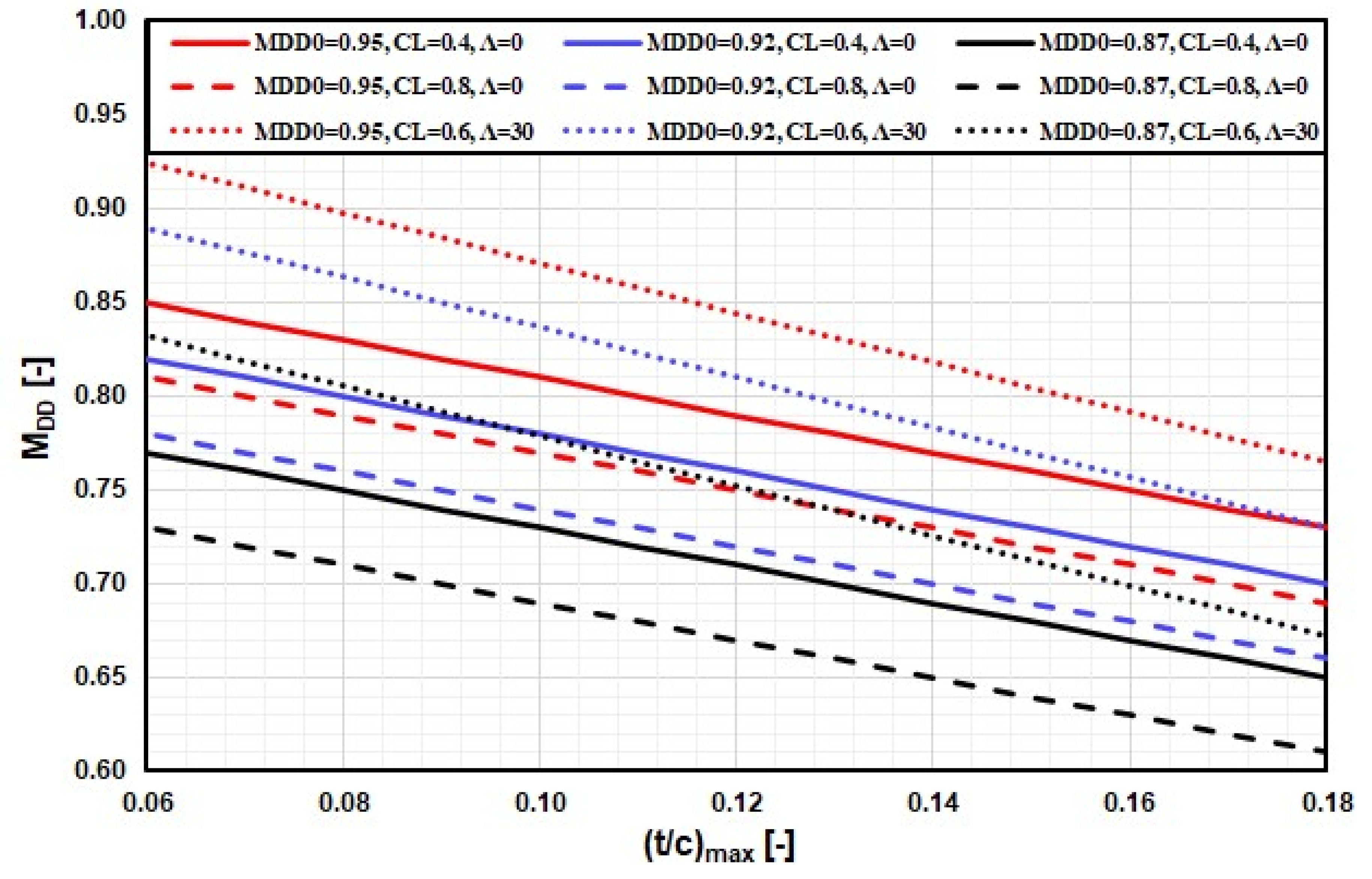
Airplane still-air ranges (SAR) are dependent on airframe, powerplant, and in-flight weights for flights at constant-altitudes. They are computed here by solving a simultaneous system of nonlinear algebraic equations for given design and flight conditions. In straight and level (S&L) flight, thrust provided by powerplants must equal aerodynamic drag (includes speed-dependent parasitic, induced, and wave drag). While parasitic and induced drag can be computed explicitly, speed-dependent wave drag must be solved by iterative numerical method. Fuel consumption is computed, and the process is repeated for various flight conditions (ISA altitudes) and weights/masses using the same airplane and powerplant models. Drag divergence Mach is computed using modified Korn’s equation for given wing/airfoil design (supercritical design, sweep angle, relative airfoil thickness, and coefficient-of-lift). The critical Mach number is computed based on modified Lock’s equation, with coefficients being variable to accommodate for specific design changes.

This fictious airplane considered here is similar to popular long-range twin B767-300ER, but there was no attempt to replicate exact performance data, nor are such data available in public domain. Basic information on virtual and fictitious testbed airplane is provided in

Table 1. Basic data for a large T-category FAR/CS 25 medium- to long-haul commercial jet.

MTOW [lb]	MLW [lb]	S [ft2]	b [ft]	AR [-]	e [-]
400,000	320,000	3100	156.0	7.85	0.90 (cruise)

and

Table 2. Aerodynamic data of the fictitious large T-category FAR/CS 25 commercial jet.

Configuration	CD,0	K	Supercritical Sections κ [-]	t/c [%]	Sweep Λ [°]	Technology Factor MDD0 [-]	Maximum Oper. Mach MMO [-]
Clean/Cruise	0.020	0.045	0.14	12	35	0.94	0.85

. Essential turbofan data [31] is presented in

Table 3. Basic data for flat-rated turbofan engines model used.

Turbofan	TSL, Static [lb] TOGA/MCT	TSFC0 (MCT) [lb/lb-hr]	n	a1	a2	Carried Fuel WFuel [lb]
HBPR	60,000/54,000	0.40	0.8	−8.5 × 10−4	+5.5 × 10−7	161,000
UHBPR	72,000/64,800	0.32	0.9	−9.5 × 10−4	+5.0 × 10−7	161,000

.

We will first compare range and SAR for the model airplane and powerplant using four different fuel laws (a–d) with and without (totally unrealistic) transonic wave drag. Subsequently, as most complex fuel-law (d) described in Equation (26) delivers most promising results, only this one will be used for further analysis to examine the effect of varying input parameters. Following introductory overview shows the cases we will present in detailed manner in the results:

• MRC range and airspeed (Figure 3 and Figure 4 and

  Table 4. Fuel law-dependence of MRC and MRC Mach number (M_MRC) for both cases, with and without transonic wave-drag model.

  	MRC (Case I)	MRC (Case II)	MRC (Case III)	MMRC (Case I)	MMRC (Case II)	MMRC (Case III)
  Without wave drag	10,036 nm	6055 nm	6049 nm	0.935	0.797	0.838
  With wave drag	9440 nm	6005 nm	5931 nm	0.797	0.763	0.778
  	(−5.9%)	(−0.8%)	(−1.9%)	(−14.8%)	(−4.2%)	(−7.2%)

  ) using fuel-laws (b), (c), and (d) (here designated as cases I, II, and III).
• MRC range and airspeed (Figure 5 and Figure 6), using fuel-law (d) only for various pressure altitudes (flight levels).
• MRC range, airspeed, and drag breakdown (Figure 7, Figure 8 and Figure 9), using fuel-law (d) for various in-flight weights.
• MRC range and airspeed (Figure 10), using fuel-law (d) for various wing planform reference surface areas.
• MRC range, airspeed, and drag breakdown (Figure 11 and Figure 12), using fuel-law (d) for various wing planform back-sweep angles.
• MRC range and airspeed (Figure 13), using fuel-law (d) for various turbofan engines BPRs.

4. Results and Discussion

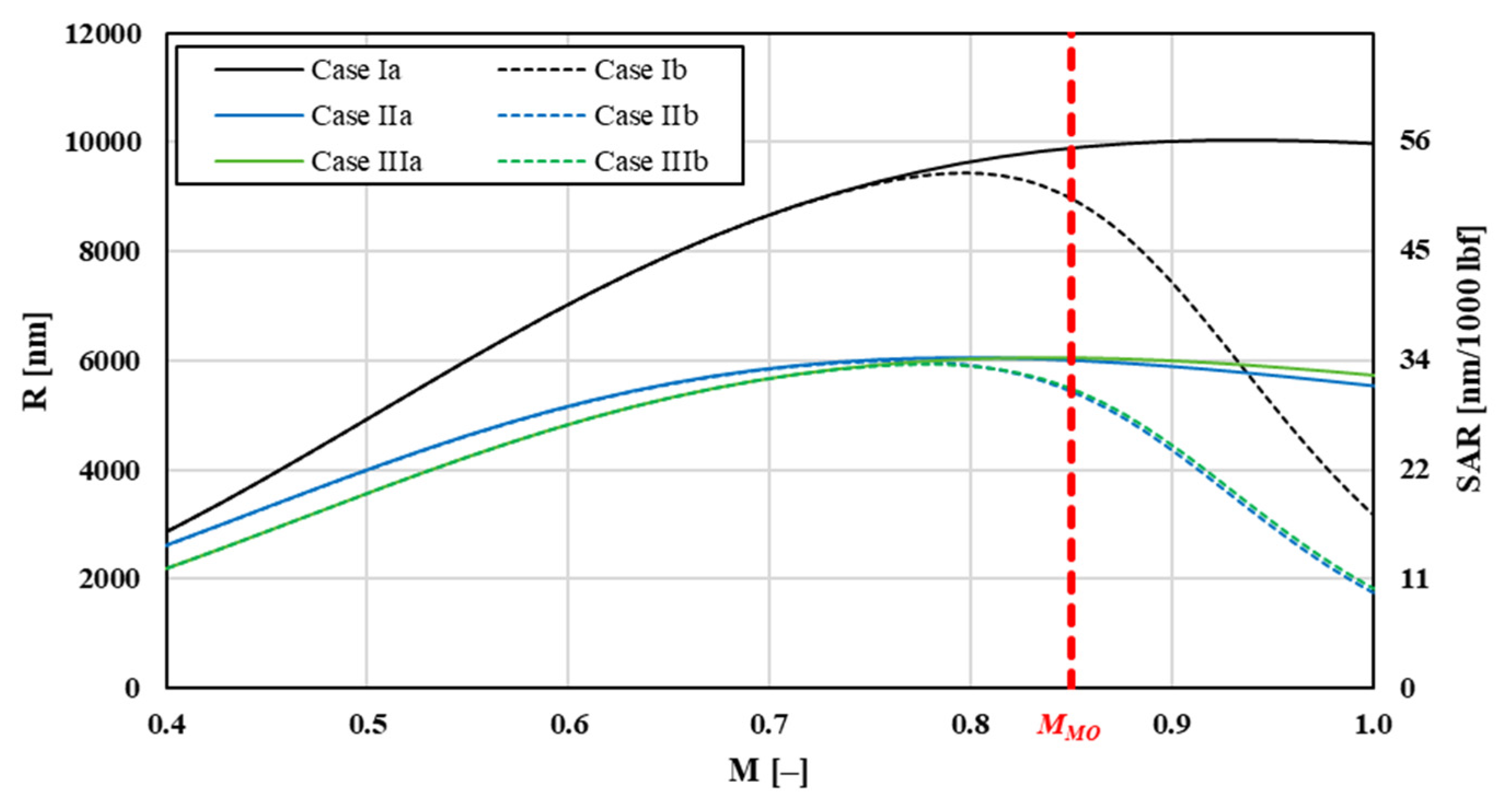
A comparison of cruise performance parameters for the three different fuel laws (b–d) introduced earlier (Equation (25)) with and without transonic wave drag (Cases I-a to III-b) is presented in Figure 3. Fuel-law (a) differs from fuel-law (b) only in range (by the square-root of temperature ratio) but not in V_MRC. A large difference exists in maximum range depending on which fuel-law is chosen. Speed-independent fuel-laws (case (b) in our classification of fuel-laws) represented in Figure 3 as I-a (no wave drag) and I-b (with wave drag) predictably result in longest computed ranges. However, that result is not realistic. Maximum range (with full fuel load) for the fictitious transport airplane modeled here would amount to over 10,000 NAM, which is about 65% longer than maximum of about 6000 NAM of a real B767-300ER aircraft. Additionally, the SAR of 56 NAM/1000 lb fuel is unrealistic and closer to values of narrow-body airplanes that cruise at SARs of 50 to 90 NAM/1000 lb fuel [30].

Cases II (fuel-law (c)) and III (fuel-law (d)) are speed-dependent and more realistic. Maximum range totals of about 6000 NAM and SAR are approximately 34 NAM/1000 lbf. These results are in good agreement with the data of existing Boeing 767-300ER and other modern wide-body airplanes of similar size. Fuel law (c) (Cases II-a and II-b) results in slightly higher performance numbers at M < 0.6. Furthermore, it is sensitive to chosen TSFC_ref. For the TSFC_ref = (1.8 × TSFC₀) used here, the results for cases II and III overlay almost exactly. For factors 1.7 or lower, range and SAR curves would shift upwards. Due to complex turbofan engine characteristics, it cannot be predicted with sufficient reliability which factor is required for each airframe-engine combination. Other authors, such as [48,52], state that fuel-law (c) is only applicable at higher Mach numbers, M ≥ 0.6. It can be reasonably assumed that the new proposed fuel law (d) (cases III-a, III-b) seems to be most reliable, accurate, and robust in predicting MRC and MRC-airspeed V_MRC in the entire flight envelope. Subsequent investigations into the influence of dynamic input parameters will therefore be mostly conducted using this new proposed fuel-law.

One can observe from Figure 3 an expected decrease in the maximum range in all cases when transonic wave drag model is included. Results start to diverge upon reaching M_CR, which in these cases is around 0.75. One can also observe relatively flat maximums, meaning that small speed variations around MRC do not affect still-air range much. Range change for speed-independent fuel law (b) is quite severe but still overpredicts range in comparison with the speed-dependent fuel laws. This is not surprising as the maximum for case I-a is located deep in the transonic speed range close to M = 1. Once wave-drag is accounted for, maximum range for cases II and III occurs at lower airspeeds of approximately M ≈ 0.8. It must be stated that the transonic wave-drag model becomes increasingly inaccurate as the freestream flight Mach number increases and especially as the upper boundary of transonic regime (M = 1.2) is approached. In the upper transonic region, shocks become stronger. However, we are only interested in the wave-drag at the lower end of the transonic region. 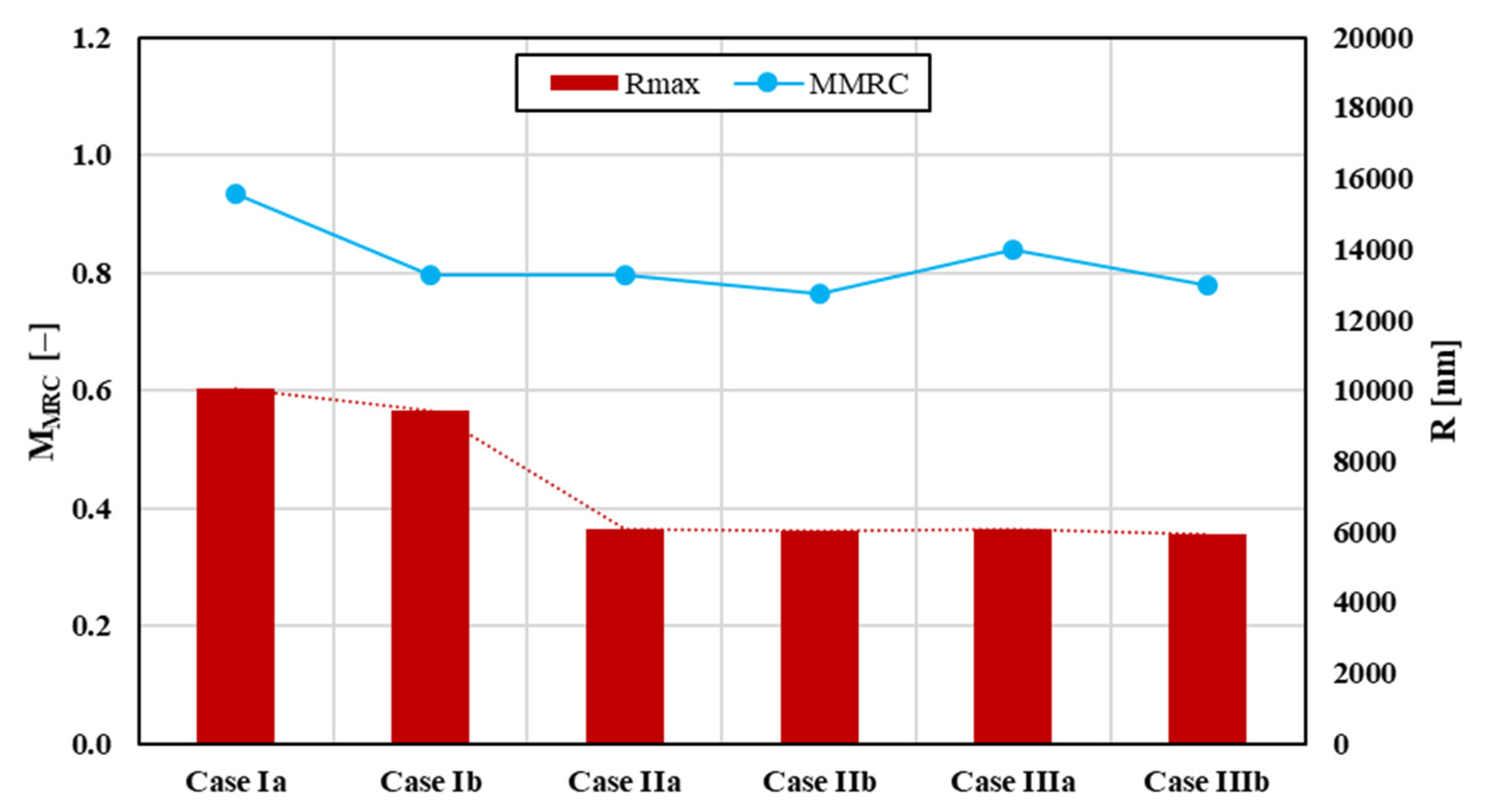Additionally, for all three cases, V_MRC decreases when the wave-drag is included. The difference is largest for fuel law “b” (−15%) and least for “c” (−4.2%) as it exhibits the earliest maximum in the range. For the fuel-law “d”, wave drag penalty on V_MRC is negative 7.2%. The exact data for fuel law comparison for the fictitious T-category airplane are summarized in Table 4 and Figure 4. Apparently, transonic wave drag has more effect on the V_MRC/M_MRC than on cruise range (MRC) itself. For all cases, MRC is obtained at airspeeds closer to drag-divergence Mach number than minimum-drag airspeed (V_MD/M_MD). Maximum cruise range M_MRC at high altitudes is usually 10–32% greater than M_MD and located in transonic range. As fuel law (d) was now identified to deliver most robust results, subsequent analysis here will only consider that fuel law. Analytical and polynomial MRC airspeeds and ranges for fuel-laws (a), (b), and (c) are summarized in Appendix A.

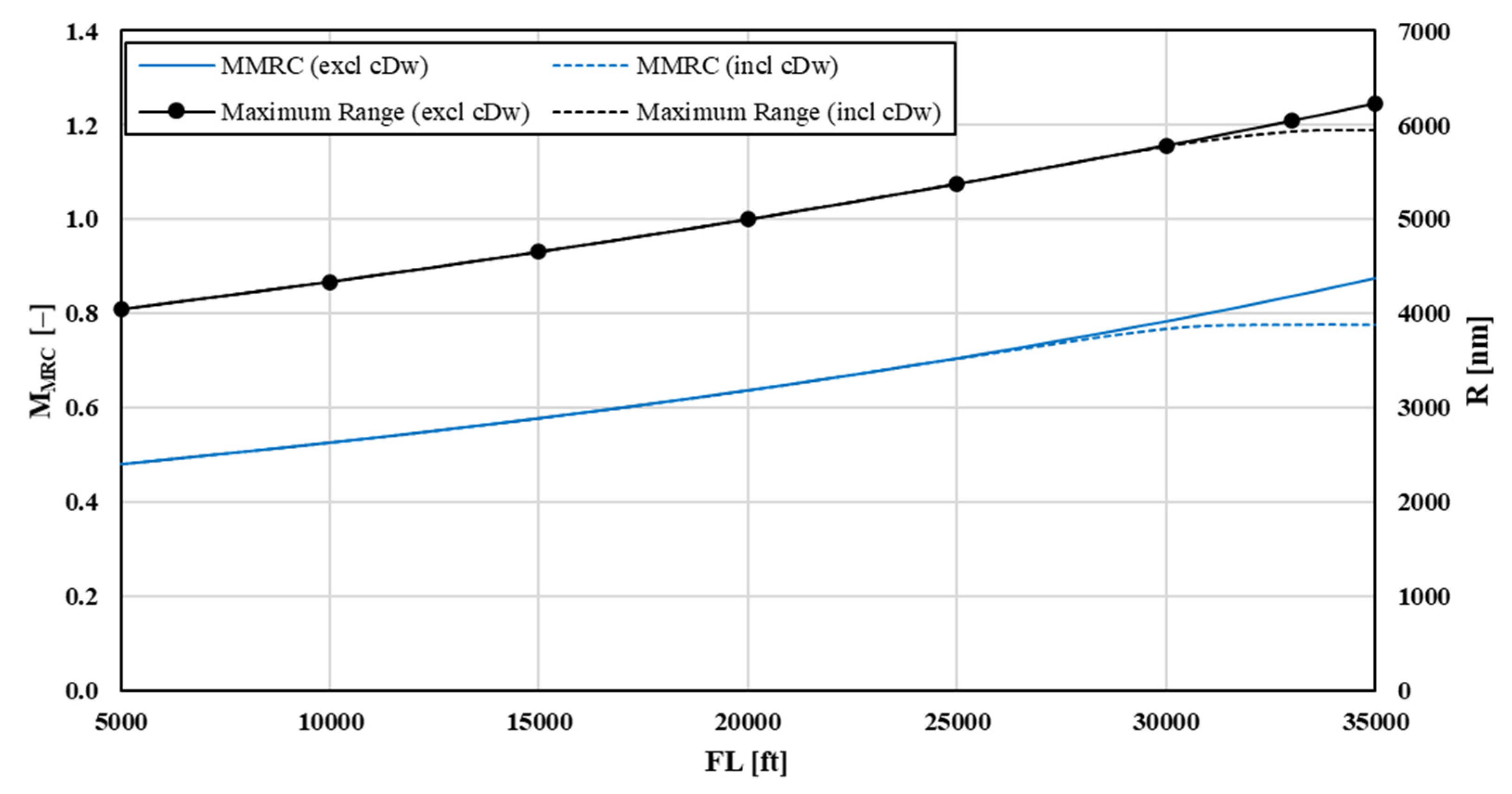
The numerical computations were performed for flight-level (FL) increments of 5000 ft (1500 m) starting at 5000 ft. Results reveal a tendency towards higher achievable range at greater altitudes and at increased airspeeds (>+40%). Wave drag must be taken into account only at typical cruise levels because, for the fictional T-category airplane modeled here, M_MRC < M_CR until up to about 28,000 ft. For flight levels where wave drag is present, it comes as no surprise that both range and MRC airspeed are located below the results when transonic wave drag is neglected. SAR changes from 22.5 NAM/1000 lb at 5000 ft to almost 33 NAM/1000 lb at FL330.

Figure 5 illustrates the behavior in the familiar two-dimensional layout, while Figure 6 resorts to a three-dimensional plot. Here, one can rapidly identify that maximum range occurs at the highest flight altitudes and at Mach numbers around 0.8. No confidence exists for the results exceeding flight Mach numbers of about 0.94 for the present model.

Further investigations were conducted for clean cruise configurations at FL330 and variable in-flight weight. Reducing in-flight weight while keeping fuel capacity constant naturally leads to increased range due to reduced vortex drag. B767-300ER with a take-off and fuel weight of about 410,000 lb and 160,000 lb, respectively, has a usable fuel fraction of 39%. This is in the range of modern transport commercial jets, which have a fuel-weight ratio of less than half their maximum structural take-off weights (about 26% for medium-haul and 45% for long-haul planes). Maximum range decreases with increased in-flight weight, and M_MRC is evaluated for both drag models, including and excluding wave drag, as shown in Figure 7. The relationship between the 1-g flight C_L and Mach at given weight and altitude (pressure ratio) is:

$$M^2{C}_L\propto \frac{W}{\delta }$$

(32)

In-depth analysis would show that the maximum still-air range will be obtained by maintaining the product M² × C_L constant, which, for decreasing in-flight weight (due to fuel consumption), will require an airplane to climb continuously at low climb rates (15–25 feet/minute). Since ATC separation traffic restrictions do not allow continuous-climb flight (except for famed Concorde’s continuous-climb at supersonic speeds), the next best thing is step-climb, which is an accepted operational practice made more feasible by introduction of RVSM [30]. 3D plot illustrating dependance of range on flight Mach number and in-flight weight is presented in Figure 8. When transonic shock systems are present, V_MRC rises to certain point. After passing “critical weight” condition, best cruise airspeed stays almost constant and decreases only slightly with increased weight. The reason for is the increasing transonic wave-drag coefficient with increasing Mach number. In cases where transonic wave drag was neglected, V_MRC increases almost linearly while range decreases. Graphical representation of drag counts as a function of weight is shown with a bar-graph in Figure 9. Even at highest weights, transonic wave drag is a very small proportion of the total drag (less than 5%).

An overview of percentage variations of maximum range and corresponding best cruise airspeed is summarized in

Table 5. Weight-dependence of maximum range and maximum-range airspeed, for both cases, with and without wave drag (including/excluding wave drag).

W [1000 lb]	300	340	380	420	460	500
Mach (M) No wave drag	0.731	0.776	0.818	0.857	0.895	0.931
Mach (M)	0.731	0.766	0.776	0.778	0.777	0.774
With wave drag	−0.0%	−1.3%	−5.1%	−9.2%	−13.2%	−16.9%
Range (R) No wave drag	8080 nm	7088 nm	6352 nm	5778 nm	5316 nm	4934 nm
Range (R)	8080 nm	7081 nm	6285 nm	5597 nm	4982 nm	4426 nm
No wave drag	−0.0%	−0.1%	−1.0%	−3.1%	−6.3%	−10.3%

. It can be concluded that lift-dependent wave drag component has significant impact on cruise performance for heavy aircraft.

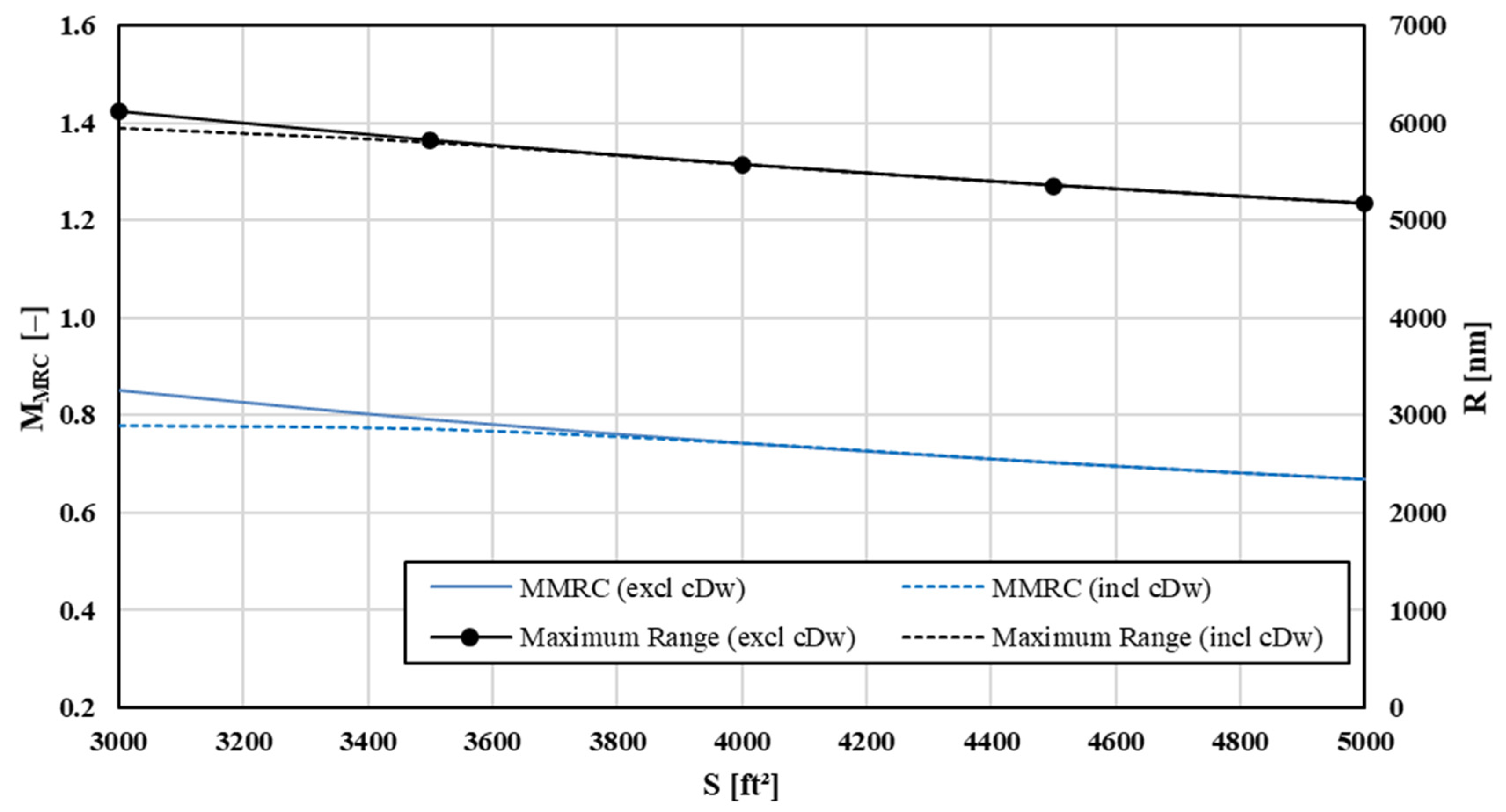
Discussion of third input parameter wing reference surface area shows that increasing surface area results in progressively lower maximum range as well as lower airplane’s best cruise speed for both models including and excluding wave drag. Larger wing surface areas effectively reduce lift coefficient C_L and cause later drag rise (higher M_DD). On the other hand, larger wing wetted area creates more parasitic drag so that most economic cruise airspeed essentially moves to lower speeds. Interestingly, wave drag only comes into account for smaller wing areas because for larger lifting surfaces V_MRC is shifted into subcritical subsonic region (M < M_CR). Consequently, no wave drag can form, and the curves for both models are identical as plotted in Figure 10.

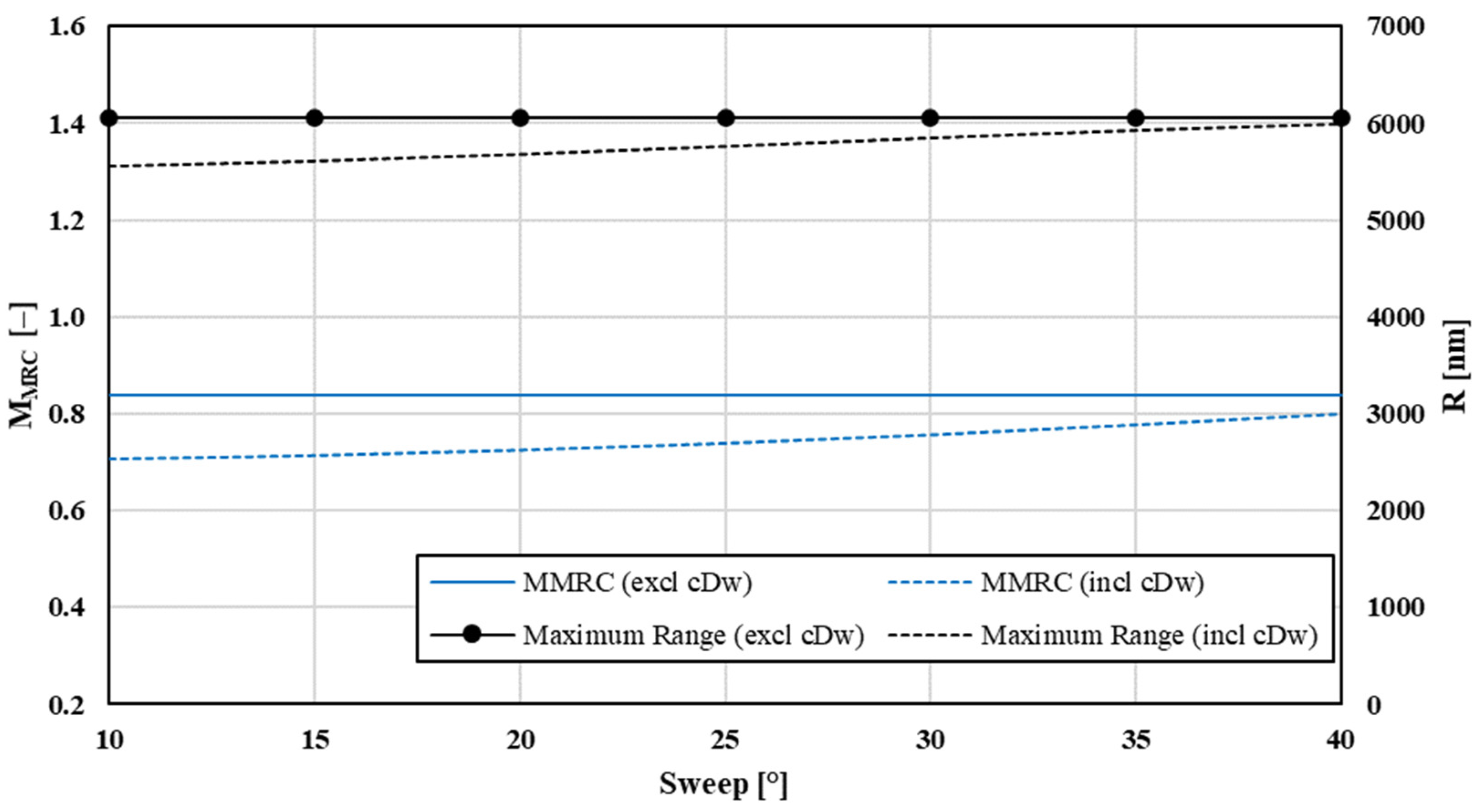
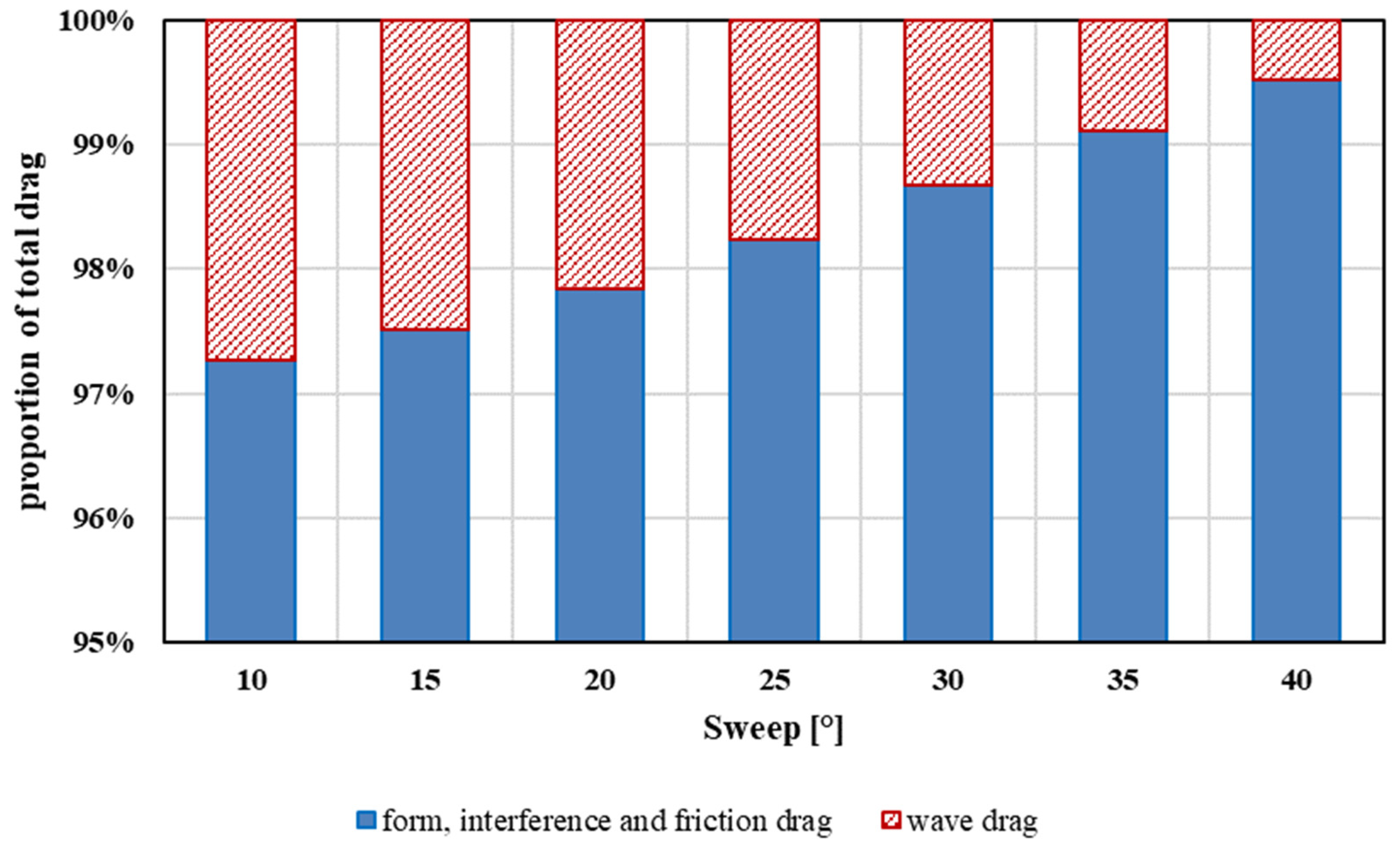
If transonic-flow normal shocks are ignored, the sweep-angle Λ parameter does not change the total drag significantly. Range and maximum cruise range airspeed remain constant in that case, as shown in Figure 11. With wave drag included, increasing leading-edge sweep delays critical flow conditions on the wing’s upper surface to higher Mach numbers as the LE perpendicular velocity component diminishes. A good example is Concorde, which, although flying supersonically, had subsonic double-ogee wing planform. Thereby, C_Dw decreases and efficient flight at higher forward speeds is enabled. Accordingly, both V_MRC and range also increase steadily with Λ (M_DD increases with increasing sweep angle according to modified Korn equation). Wave drag decreases with increased sweep, a relation that is noticeable also with the drag proportions in Figure 12 and range and M_MRC data presented in

Table 6. Maximum range and best cruise airspeed for both models, with and without wave drag.

Λ [degree]	10°	15°	20°	25°	30°	35°	40°
M [-] No CDw	0.838
M [-]	0.707	0.715	0.725	0.740	0.757	0.778	0.800
With CDw	−15.6%	−14.7%	−13.4%	−11.7%	−9.6%	−7.2%	−4.5%
R [NAM] No CDw	6049 nm (11,200 km)
R [NAM]	5554	5608	5679	5762	5849	5931	5995
With CDw	−8.2%	−7.3%	−6.1%	−4.7%	−3.3%	−1.9%	−0.9%

.

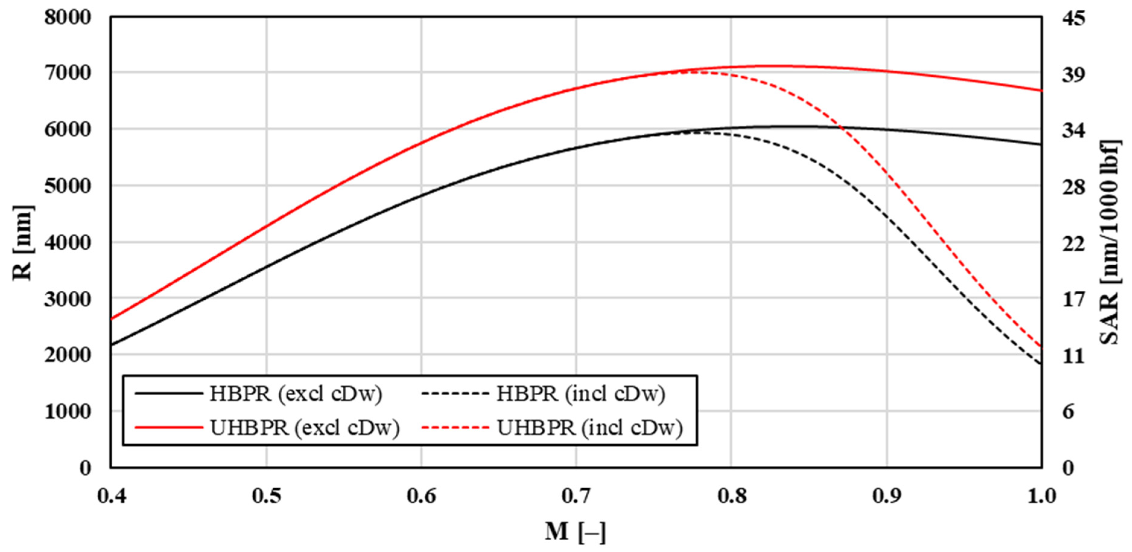
The last input parameter evaluated here is BPR of turbofan engines. Aircrafts equipped with powerplants with higher BPR tend to achieve greater range due to lower TSFC. However, the airspeed V_MRC at which optimum range is reached stays almost constant for HBPR (High BPR) and UHBPR (Ultra-High BPR) engines. At high Mach numbers between 0.8 and 0.9, UHBPR turbofans show a larger thrust decrease due to ram effect than HBPR engines. Cruise altitudes such as FL330 result in only a minor difference in thrust available for both turbofan types, and consequently both V_MRC are nearly identical. If one considers other engines than the P&Ws PW4056 modeled here with Equation (24), a greater BPR would accentuate the trend towards better range performance. The higher the BPR, the higher maximum range at still almost constant M_MRC, as shown in Figure 13.

All previous computations and optimizations were made for the AEO (All Engines Operating) cruise scenarios. OEI (One Engine Inoperative) conditions were treated for all input parameters, but it was found that they do not require separate presentation as the maximum level airspeeds when OEI are significantly lower than for the AEO cases. Sudden engine failure in flight is not a particularly serious problem as the aircraft will continue to fly; however, a drift-down must be initiated toward OEI-service ceiling (typically 22,000–25,000 ft) where flight at constant airspeed can be maintained with remaining operating engine(s). OEI maximum range cruise airspeed will no longer be in transonic region and hence no wave drag is present. Additionally, flight may proceed to unscheduled nearest acceptable airport. For more details on optimal subsonic airspeeds and range during OEI conditions, one can resort to [31].

Looking at the fictional aircraft modeled here with MTOW of 400,000 lb, sweep of 35°, wing area of 3100 ft² and in cruise at FL330, wave drag accounts for only 1% of the total drag when flying at MRC Mach number of about 0.78. Drag breakdowns are also shown in Figure 9 and Figure 12. However, many references estimate the transonic wave drag component for transport airplanes flown at cruise M below M_DD at about 5% of the total drag [53,54]. This discrepancy cannot be ascribed to deficiencies of the mathematical model but finds its origin primarily in two contributing factors. Firstly, the sweep angle of 35° used here is rather high. Real B767-300ER, A350, and similar T-category airplanes feature leading edges with angles of 31.5 to 32°. Secondly, long-range jetliners will normally cruise at speeds faster than M_MRC. The cost index (CI) is practically never zero in flight operations, and time-cost (crew time, etc.) plays an important role in finding best-economy airspeed. Flying with effective headwinds will require faster forward airspeeds to maximize range over ground or SGR [30]. While M_MRC does not account for wind, economy-Mach (M_ECON) does. Modern T-category jets are sometimes flown at the long-range-cruise airspeed (M_LRC) industry standard, which is based on the 99% MRC, which corresponds to somewhat higher LRC airspeeds (M_LRC is typically M_MRC + 0.02). For our fictious airplane model, M_MRC is 0.78 so that M_LRC could be about 0.80 (which also happens to be design cruise Mach of B767-300). Wave drag and the total C_D for new sweep and forward airspeed would amount to 0.00148 and 0.03395, respectively. Wave drag proportion of the total drag is now 4.4% and close to the usual cited figures of 5% for high-subsonic wide-body airplanes, again validating the accuracy of the approach in this study. Using Flight Management Systems (FMS), the operational airspeeds are economy Mach numbers, which minimizes total operating cost (fuel-cost and time-dependent cost). For more details on cruise speeds, ranges, and economy, see [30].

Maximum operating limit airspeeds in flight operations V_MO/M_MO are based on flight testing and are established in relationship to design diving airspeed V_D/M_D, maximum flight demonstrated diving airspeed V_DF/M_DF, and the maximum airspeed for stability characteristics V_FC/M_FC. Some of the corresponding regulations in US are Title 14 of CFR 25.253 (high-speed characteristics), CFR 25.335 (design airspeeds), and CFR 25.1505 (maximum operating limit airspeed). Maximum operating limit airspeed is limited by max-q (at lower altitudes) and generally by aircraft static and dynamic stability, control, handling qualities, upset recovery, structural integrity, flutter, vibrations, loads, and other limitations. More on this subject and airworthiness requirements of FAR and CS 25 airplanes can be found in [55,56,57]. Range is computed and summarized in

Table 7. Flight Mach, maximum still-air range, and wave-drag percentage of the total drag for various flight conditions at constant in-flight weight of 350,000 lb flying at 35,000 ft ISA.

	M > MCR	MMRC	MLRC	MECON	MDD	MMO
		CI = 0	CI ≈ 30–40	CI ≈ 80	CI ≈ 140	CI ≈ 200
Flight Mach [-]	0.77	0.78	0.80	0.82	0.84	0.85
Air-Range [NAM]	7006 nm	7010	6950	6857	6655	6488
	−0.06%	−0.14%	−1.0%	−2.18%	−5.06%	−7.47%
Wave Drag [%]	0.41%	0.71	1.88	3.37	6.15	8.38

for various aerodynamic, performance, control, and operationally limiting airspeeds for an airplane similar to B767-300 (check Table 1, Table 2 and Table 3). Approximate operational cost index (CI) for a typical range 0–200 (in older FMSs) was given as a reference. In these conditions, critical Mach number is about 0.75 with the wave drag being zero. Still-air range at M_CR is lower than at M_MRC. Values of wave drag proportion, airspeeds, and ranges agree well with the certified and flight-tested values for T-category airplanes of similar designs, demonstrating that modeling used here is reasonably accurate.

It must be underscored again that transonic wave-drag represents complicated flow phenomenon that cannot be fully described by a relatively simple semi-empirical algebraic model in the supercritical flight regime as used here. For Mach numbers between M_CR and M_MO as investigated in this study, the proposed semi-empirical wave-drag, fuel-law, and turbofan models are still reasonably satisfactory and could be used to develop basic methodology for design optimization in early aircraft development phases. During such initial phase, other performance airspeeds under control of wave-drag can be estimated with the present model, such as the maximum level-flight propulsion-limited airspeed. Computations of propulsion-limited maximum level flight airspeeds may be presented in a separate publication. It is also emphasized that this is perhaps one of several possible methodologies of estimating cruise parameters of modern transonic airplanes. The results obtained here show reasonable agreement with demonstrated flight data. Further improvements in models are possible and are envisioned. Present algebraic models could be, in theory, extended to account for supersonic flight of various aerospace designs. One of the biggest difficulties in presented method is in choosing a wing-technology factor for a given design as no rational analysis for that currently exists.

5. Conclusions

Transonic wave-drag computations using modern RANS/LES/DNS codes is time, cost, and resource consuming. Thus, in this article a semi-empirical wave-drag model for supercritical flow was developed and subsequently added to the standard compressible subcritical parabolic drag polar in the linear lift region. The wave drag model developed is increasingly inaccurate for Mach numbers approaching one and should be fully discarded for Mach numbers on supersonic side of the transonic regime. Luckily, only the subsonic side of the transonic supercritical flow around the drag-divergence Mach number was needed. The criterion of maximizing the specific air range (SAR) was developed. Optimality criterion delivers polynomials, whose analytical and numerical solutions agree well with the known cruise range and airspeed results of modern commercial T-category jets. New semi-empirical turbofan model and fuel-laws were implemented, giving rise to polynomials of 12th and higher orders. A numerical Newton–Raphson nonlinear equation solver code was developed and used for all computations. The NR algorithm searched only for positive real roots of polynomials representing the sought-after optimum airspeeds. The NR method and code were extensively tested against known analytical cruise range solutions to guarantee accuracy and convergence. Cruise range is calculated by analytical or numerical integration of Breguet range equation while utilizing several fuel-flow laws for comparison. It was found that transonic shock systems have a noticeable influence on cruise range parameters. The dependence of performance airspeeds on several design features was explored for a specific airframe-powerplant vehicle and various atmospheric cruise conditions.

The numerical method used can be applied to all other drag polynomials, including eventual non-integer exponents. If available, wind tunnel-, flight-test-, or CFD-obtained transonic drag polars can be incorporated into methodology developed. The model used here allows turbofan characteristics in any suitable polynomial form. It can be utilized to identify the most beneficial input parameter values and combinations for the cruise flight phase, especially regarding geometric airframe data. The algorithm represents a powerful tool to estimate important performance airspeeds in transonic flights on the subsonic side. Its intended application is utilization in the conceptual development stages of the design optimization of high-subsonic jet airplanes. The results may also assist in improving operational techniques and best piloting practices in modern air transportation. Further improvements of this integral algebraic model are certainly possible and are planned.

References

1. Chapman, D.R. Computational Aerodynamics Development and Outlook. AIAA J. 1979, 17, 1293–1313. [Google Scholar] [CrossRef]
2. Johnson, F.T.; Tinoco, E.N.; Yu, N.J. Thirty years of development and application of CFD at Boeing Commercial Airplanes, Seattle. Comput. Fluids 2005, 34, 1115–1151. [Google Scholar] [CrossRef] [Green Version]
3. Drikakis, D.; Kwak, D.; Kiris, C.C. Computational aerodynamics: Advances and challenges. Aeronaut. J. 2016, 120, 13–36. [Google Scholar] [CrossRef] [Green Version]
4. Spalart, P.R.; Venkatakrishnan, V. On the role and challenges of CFD in the aerospace industry. Aeronaut. J. 2016, 120, 209–232. [Google Scholar] [CrossRef] [Green Version]
5. Mason, W. On the use of the potential flow model for aerodynamic design at transonic speeds. In Proceedings of the 33rd Aerospace Sciences Meeting and Exhibit (AIAA 95-0741), Reno, NV, USA, 9–12 January 1995. [Google Scholar]
6. Fujino, M.; Kawamura, Y. Wave-Drag Characteristics of an Over-the-Wing Nacelle Business-Jet Configuration. J. Aircr. 2003, 40, 1177–1184. [Google Scholar] [CrossRef] [Green Version]
7. Cole, J.D.; Malmuth, N.D. Wave drag due to lift for transonic airplanes. Proc. R. Soc. A Math. Phys. Eng. Sci. 2005, 461, 541–560. [Google Scholar] [CrossRef]
8. Jameson, A.; Ou, K. 50 years of transonic aircraft design. Prog. Aerosp. Sci. 2011, 47, 308–318. [Google Scholar] [CrossRef]
9. Chaouat, B. The State of the Art of Hybrid RANS/LES Modeling for the Simulation of Turbulent Flows. Flow Turbul. Combust. 2017, 99, 279–327. [Google Scholar] [CrossRef] [PubMed] [Green Version]
10. Hilton, W.F. High Speed Aerodynamics; Longmans & Co.: London, UK, 1951. [Google Scholar]
11. Hankey, W.L.; Holden, M.S. Two-Dimensional Shock-Wave Boundary Layer Interactions; AGARD-AG-203; NATO: Neuilly sur Seine, France, 1975. [Google Scholar]
12. Délery, J.; Dussauge, J.-P. Some physical aspects of shock wave/boundary layer interactions. Shock Waves 2009, 19, 453–468. [Google Scholar] [CrossRef]
13. Houghton, E.L.; Carpenter, P.W. Aerodynamics for Engineering Students, 5th ed.; Butterworth Heinemann: Oxford, UK, 2003. [Google Scholar]
14. Landau, L.D.; Lifshitz, E.M. Fluid Mechanics (Volume 6—Course of Theoretical Physics), 2nd ed.; Translation from Russian; Pergamon Press: Oxford, UK, 1987. [Google Scholar]
15. Zel’dovich, Y.B.; Raizer, Y.P. Physics of Shock Waves and High-Temperature Hydrodynamic Phenomena; 1966 and 1967 Translation from Russian; Hayes, W.D., Probstein, R.F., Eds.; Dover: Mineola, NY, USA, 2002; Volume 2. [Google Scholar]
16. Hayes, W.D.; Probstein, R.F. Hypersonic Inviscid Flow; Dover: Mineola, NY, USA, 2003. [Google Scholar]
17. Anderson, J.D., Jr. Hypersonic and High-Temperature Gas Dynamics, 2nd ed.; AIAA: Reston, VA, USA, 2006. [Google Scholar]
18. Miele, A. Flight Mechanics: Theory of Flight Paths; Dover: Mineola, NY, USA, 2016. [Google Scholar]
19. Küechemann, D. The Aerodynamic Design of Aircraft; AIAA: Reston, VA, USA, 2012. [Google Scholar]
20. Shevell, R.S. Fundamentals of Flight; Prentice Hall: Englewood Cliffs, NJ, USA, 1989. [Google Scholar]
21. Menon, P.K.A. Study of aircraft cruise. J. Guid. Control. Dyn. 1989, 12, 631–639. [Google Scholar] [CrossRef]
22. Miller, L.E. Optimal cruise performance. J. Aircr. 1993, 30, 403–405. [Google Scholar] [CrossRef]
23. Malone, B.; Mason, W.H. Multidisciplinary optimization in aircraft design using analytic technology models. J. Aircr. 1995, 32, 431–438. [Google Scholar] [CrossRef]
24. Torenbeek, E. Cruise performance and range prediction reconsidered. Prog. Aerosp. Sci. 1997, 33, 285–321. [Google Scholar] [CrossRef]
25. Mason, W.H. Transonic aerodynamics of airfoils and wings. In AOE 4124 Configuration Aerodynamics Lecture Notes; Virginia Polytechnic Institute and State University: Blacksburg, VA, USA, 2002; Available online: http://www.aoe.vt.edu/~mason/Mason_f/ConfigAeroTran-sonics.pdf (accessed on 22 August 2021).
26. Jakirlić, S.; Eisfeld, B.; Jester-Zürker, R.; Kroll, N. Near-wall, Reynolds-stress model calculations of transonic flow configurations relevant to aircraft aerodynamics. Int. J. Heat Fluid Flow 2007, 28, 602–615. [Google Scholar] [CrossRef]
27. Friedewald, D. Numerical Simulations on Unsteady Nonlinear Transonic Airfoil Flow. Aerospace 2020, 8, 7. [Google Scholar] [CrossRef]
28. Cavcar, M.; Cavcar, A. Approximate solutions of range for constant altitude–constant high subsonic speed flight of transport aircraft. Aerosp. Sci. Technol. 2004, 8, 557–567. [Google Scholar] [CrossRef]
29. Rivas, D.; Valenzuela, A. Compressibility Effects on Maximum Range Cruise at Constant Altitude. J. Guid. Control Dyn. 2009, 32, 1654–1658. [Google Scholar] [CrossRef]
30. Daidzic, N. Achieving global range in future subsonic and supersonic airplanes. Int. J. Aviat. Aeronaut. Aerosp. 2014, 1, 1–29. [Google Scholar] [CrossRef] [Green Version]
31. Daidzic, N.E. Estimation of performance airspeeds for high-bypass turbofans equipped transport-category airplanes. J. Aviat. Technol. Eng. (JATE) 2016, 5, 27–50. [Google Scholar] [CrossRef] [Green Version]
32. Daidzic, N.E. High-elevation equatorial catapult-launched RBCC SSTO space-plane for manned economic access to LEO. Int. J. Aviat. Aeronaut. Aerosp. 2016, 3, 1–57. [Google Scholar] [CrossRef] [Green Version]
33. Fusaro, R.; Vercella, V.; Ferretto, D.; Viola, N.; Steelant, J. Economic and environmental sustainability of liquid hydrogen fuel for hypersonic transportation systems. CEAS Space J. 2020, 12, 441–462. [Google Scholar] [CrossRef]
34. Viola, N.; Roncioni, P.; Gori, O.; Fusaro, R. Aerodynamic Characterization of Hypersonic Transportation Systems and Its Impact on Mission Analysis. Energies 2021, 14, 3580. [Google Scholar] [CrossRef]
35. Anderson, J.D., Jr. Modern Compressible Flow: With Historical Perspective, 3rd ed.; McGraw-Hill: New York, NY, USA, 2003. [Google Scholar]
36. Ashley, H.; Landahl, M. Aerodynamics of Wings and Bodies; Dover: Mineola, NY, USA, 1985. [Google Scholar]
37. Holst, T.L. Transonic flow computations using nonlinear potential methods. Prog. Aerosp. Sci. 2000, 36, 1–61. [Google Scholar] [CrossRef] [Green Version]
38. Liepmann, H.W.; Roshko, A. Elements of Gasdynamics; Dover: Mineola, NY, USA, 2001. [Google Scholar]
39. Moran, J. An Introduction to Theoretical and Computational Aerodynamics; Dover: Minneola, NY, USA, 2003. [Google Scholar]
40. Kuethe, A.M.; Schetzer, J.D. Foundations of aerodynamics, 2nd ed.; John Wiley & Sons: New York, NY, USA, 1959. [Google Scholar]
41. von Karman, T. Compressibility Effects in Aerodynamics. J. Aeronaut. Sci. 1941, 8, 337–356. [Google Scholar] [CrossRef]
42. Tsien, H.-S. Two-Dimensional Subsonic Flow of Compressible Fluids. J. Aeronaut. Sci. 1939, 6, 399–407. [Google Scholar] [CrossRef]
43. Laitone, E.V. New Compressibility Correction for Two-Dimensional Subsonic Flow. J. Aeronaut. Sci. 1951, 18, 350. [Google Scholar] [CrossRef]
44. Batchelor, G.K. An Introduction to Fluid Dynamics; Cambridge University Press: Cambridge, UK, 2000. [Google Scholar]
45. Drela, M. Flight Vehicle Aerodynamics; MIT Press: Cambridge, MA, USA, 2014. [Google Scholar]
46. Vallone, M. Parameter Estimation of Fundamental Technical Aircraft Estimation Applied to Aircraft Performance. Master’s Thesis, California Polytechnic State University, San Luis Obispo, CA, USA, 2010. [Google Scholar]
47. Hanke, C.R.; Nordwall, D.R. The Simulation of the Jumbo-Jet Aircraft, Vol. 2: Modelling Data; NASA CR-114494; NASA ARC (Ames Research Center): Moffett Field, CA, USA, 1970. [Google Scholar]
48. Mair, W.A.; Birdsall, D.L. Aircraft Performance; Cambridge University Press: Cambridge, UK, 1992. [Google Scholar]
49. Filippone, A. Advanced Aircraft Flight Performance; Cambridge University Press (CUP): Cambridge, UK, 2012. [Google Scholar]
50. Harris, C.D. NASA Supercritical Airfoils: A Matrix of Family-Related Airfoils; NASA TP-2969; NASA LRC (Langley Research Center): Hampton, VA, USA, 1990. [Google Scholar]
51. Daidzic, N.E. Efficient general computational method for estimation of standard atmosphere parameters. Int. J. Aviat. Aeronaut. Aerosp. 2015, 2, 1–37. [Google Scholar] [CrossRef]
52. Eshelby, M.E. Aircraft Performance: Theory and Practice; Elsevier: Boston, MA, USA, 2000. [Google Scholar]
53. Anderson, J.D., Jr. Aircraft Performance and Design; McGraw-Hill: New York, NY, USA, 1999. [Google Scholar]
54. Bertin, J.J.; Cummings, R.M. Aerodynamics for Engineers, 5th ed.; Pearson Prentice Hall: Upper Saddle River, NJ, USA, 2009. [Google Scholar]
55. Federal Aviation Administration (FAA). Flight Test Guide for Certification of Transport Category Airplanes (Advisory Circular AC 25-7D, 05/04/2018); Federal Aviation Administration: Washington, DC, USA, 2018. [Google Scholar]
56. Federal Aviation Administration (FAA). Part 25, Airworthiness Standards: Transport Category Airplanes (Last Amended on 11/03/2021); Federal Aviation Administration: Washington, DC, USA, 2021. [Google Scholar]
57. European Aviation Safety Agency (EASA). Certification Specifications and Acceptable Means of Compliance for Large Aeroplanes (CS-25, Amendment 27, 24 November 2021); European Aviation Safety Agency: Cologne, Germany, 2021. [Google Scholar]
Figure 1. Computed airplane’s total drag coefficient as a function of Mach and coefficient-of-lift.
Aerospace 09 00192 g001
Figure 2. Drag-divergence Mach as a function of wing-technology factor, wing’s maximum relative-thickness, coefficient-of-lift, and sweep-angle using modified Korn’s equation.
Aerospace 09 00192 g002
Figure 3. Range and SAR of the fictional T-category high-subsonic jet airplane for three different fuel laws, with each model including and excluding transonic wave drag CDw.
Aerospace 09 00192 g003
Figure 4. MRC and MRC airspeed for three fuel-laws tested—(b), (c), and (d)—for both cases, with and without transonic wave-drag model.
Aerospace 09 00192 g004
Figure 5. MMRC and range for different FLs for both models, with/without wave drag.
Aerospace 09 00192 g005
Figure 6. 3D plot visualizing the influence of altitude and Mach on range with transonic wave drag model.
Aerospace 09 00192 g006
Figure 7. MMRC and range for variable in-flight weight for both drag models, with and without transonic wave drag.
Aerospace 09 00192 g007
Figure 8. 3D plot visualizing influence of in-flight weight and Mach number on the range, including transonic wave drag.
Aerospace 09 00192 g008
Figure 9. Drag breakdown for a simulated fictitious T-category aircraft, depending on in-flight cruise weight.
Aerospace 09 00192 g009
Figure 10. MMRC and range over wing surface area for both models, including and excluding CDw.
Aerospace 09 00192 g010
Figure 11. MMRC and range for variable sweep angle Λ for both models, with and without CDw.
Aerospace 09 00192 g011
Figure 12. Drag breakdown of a fictitious T-category airplane as a function of sweep angle Λ.
Aerospace 09 00192 g012
Figure 13. Range and SAR of the fictitious T-category airplane as a function of BPR and Mach number for both models, including and excluding wave drag.
Aerospace 09 00192 g013