Article

Unmanned Aircraft Collision Detection and Avoidance for Dealing with Multiple Hazards

Italian Aerospace Research Center (CIRA S.c.P.A.), 81043 Capua, Italy
*
Author to whom correspondence should be addressed.
Aerospace 2022, 9(4), 190; https://doi.org/10.3390/aerospace9040190
Submission received: 22 February 2022 / Revised: 28 March 2022 / Accepted: 28 March 2022 / Published: 1 April 2022
(This article belongs to the Special Issue Recent Advances in See and Avoid Systems for Aircraft)

Abstract

:
Collision Detection and Avoidance is one of the critical technologies for fully allowing Unmanned Aerial Systems to fly in civil airspaces. Current methods evaluate only potential conflicts with other aircraft using specific parameters (e.g., time or distance to closest point of approach) that can only be used for pair-wise encounters, not considering the surrounding environment. The present work proposes a new Collision Detection and Avoidance concept to solve short-term conflicts in scenarios characterized by the simultaneous presence of aircraft and other path constraints (i.e., no-fly zones, bad weather areas and terrain) including geo-fencing limitations. Differently from other open literature methods, the proposed algorithm computes two parameters that synthetically describe the conflict hazard level of a given scenario and its possible evolution, independently from the type and the number of surrounding potential threats. Using such indices, a risk evaluation strategy is proposed that detects hazardous situations and generates an optimal maneuver avoiding potential collisions while not causing secondary conflicts. The effectiveness of the proposed algorithm is demonstrated by means of fast-time and real time simulations in some challenging conflict scenarios that cannot be solved by state of the art Detect and Avoid systems.

1. Introduction

The operational concept defined by the International Civil Aviation Organization (ICAO) [1] specifies that the air traffic system shall have a conflict management process for limiting, to an acceptable level, the risk of collision between aircraft and other potential hazards. This conflict management process has three layers: strategic, tactical, and collision avoidance. The strategic layer manages the density/complexity of traffic and this is typically performed by the Air Traffic Management authorities. The tactical layer has the objective to keep traffic safely separated from each other and other hazards in medium- to long-term encounters and it is the responsibility of air traffic controllers and pilots, depending on the situation. The collision avoidance layer, finally, addresses short-term conflicts solving emergency situations where the tactical layer failed for some reason. The implementation of such layers varies across different airspace classes and types of operations.
In this framework, the Detect and Avoid (DAA) system represents a critical component of a Remotely Piloted Aircraft Systems (RPAS) or Unmanned Aerial Vehicle (UAS) to support the remote pilot in the tactical level process (Remain Well Clear) and implement the collision avoidance function [2]. However, DAA technologies have not yet achieved a level of maturity sufficient to guarantee a so-called equivalent level of safety [3] with respect to manned aircraft, as it is demonstrated by the several active development projects all over the world. Indeed, NASA and FAA have just completed their UAS in the NAS project (in 2020) while Europe (with EUDAAS project), Canada and Australia have still active DAA development projects. Despite other limitations of current DAA design that are discussed later on in this paper, some of the key technological gaps are related to the effectiveness of such systems with small unmanned aircraft having poor performance, to the reliability and accuracy of surveillance sensors for aircraft without transponders (e.g., radar, cameras, etc.) and to the DAA processing algorithms that could be not effective in some situations with the presence of multiple maneuvering intruders. This obviously poses operational restrictions to UAS that limit their full adoption in civil airspaces.
Nevertheless, DAA system technical standards are already being prepared by several working groups such as EUROCAE WG105 in Europe, and RTCA SC-228 in U.S.A. The former published the Operational Services and Environment Description (OSED) for DAA [4] while the latter the Minimum Operational Performance Standards (MOPS) for DAA systems, referred to as Phase 1 MOPS [5]. Moreover, other technical standards have just been published or are being prepared for the ACAS-X family of collision avoidance system for different manned and unmanned vehicles with different performances. In both such technical standards and in other related specifications, DAA systems are defined only considering air traffic (not the surrounding environment), and furthermore a remote pilot is always present to supervise the flight.
In this framework, the Italian Aerospace Research Center (CIRA) is also developing a DAA system prototype, named ADAPT (Advanced Detect and Avoid ProTotype) [6], as part of a national funded research program on fully autonomous aerospace vehicles (PRORA). ADAPT includes a Collision Detection and Avoidance (CDA) function that leverages and extends some results of the most recent projects and research activities on the subject [7,8,9,10,11,12,13], trying to overcome some of the above-mentioned limitations of DAA systems.
The present work merges the results included in [14], where a collision avoidance algorithm for air traffic has been proposed, with the concepts introduced in [15] for dealing with fixed obstacles (i.e., no-fly zones, terrain and hazardous weather areas) and geo-fencing constraints. With respect to above referenced papers, this paper presents a comprehensive description of the proposed CDA algorithm and adds several details about the specific techniques that are used for evaluating the most critical algorithm variables.
Moreover, the procedures for tuning the algorithm parameters and the results obtained on some sample cases using both Fast Time Simulations and Real Time Simulations are reported.

2. Requirements of a Collision Detection and Avoidance System

The high-level requirements that describe a CDA system can be found both in documents from ICAO [3] and in other technical standards, such as [4,5,12]. The final aim of this system is to reduce the risk of collisions between aircraft flying in the civil airspace under some given values, so as to increase the safety of flight. However, given the future introduction of unmanned aircraft in routine aeronautical airspace operations, several discussions on such safety criteria and related thresholds are still in progress. Nevertheless, it is possible to list some basic features that describe at very high level a CDA system to be integrated in both manned and unmanned aircraft, as follows.
  • Minimizing the probability of entering Near Mid Air Collision (NMAC) standard volume (Figure 1) by performing an automatic maneuver (in the case of unmanned aircraft), in any airspace class.
  • Minimizing the occurrence of false alerts (nuisance) and not necessary avoidance maneuvers.
  • Being acceptable to (remote) pilots by giving clear and stable indications on the current traffic situation and on the resolution maneuver, so that the pilot can decide to manually execute it.
  • Supporting the (remote) pilot by providing alerts in case of potential conflicts with other aircraft (i.e., entering the NMAC volume).
  • Correctly performing in the presence of more than one intruder, up to a pre-defined maximum, even with several simultaneous potential conflicts.
  • Being compatible with other aircraft with the same CDA system (auto-compatibility).
Other than the above basic requirements, some other special features should be specifically considered for unmanned aircraft, as listed below.
  • Being interoperable with the current legacy Collision Avoidance system (TCAS-II, see the next section).
  • Being compliant with Right-of-Way rules, if not detrimental to flight safety.
  • Dealing with both cooperative and non-cooperative traffic by correctly processing and fusing measurements and related accuracies of different surveillance sensors.
  • Accounting for vehicle flight envelope and maneuvering limitations using a limited set of easily retrievable parameters (vehicle agnostic), so being, in principle, easily adapted to any unmanned vehicle class, without performing any specific parameter tuning and/or algorithm modification when changing the vehicle performances.
  • Correctly performing even in presence of terrain, fixed obstacles, no-fly zones and bad weather.
As it will be clearer in the subsequent sections, the last two requirements are not always considered in the current CDA algorithmic designs, so justifying the development proposed in this paper.

3. Background

Collision Detection and Avoidance for manned vehicles is a research topic that has been investigated since the late 1950s. This research was pushed by some accidents in which airliners experienced near mid-air collisions. After some years of developments, the Traffic Collision Avoidance System (TCAS-II) was introduced in late 1980s [12]. This is still the only CDA system currently commercialized and mandatorily installed on-board almost all commercial aircraft.
For these reasons, this system is the reference design for CDA algorithms, also for unmanned vehicles because it has been specified as the baseline CDA system in the Phase 1 MOPS [5].
TCAS-II systems use deterministic state projection from a single traffic surveillance sensor based on active radio interrogation and reply from the intruder. Therefore, in this system, the intruder aircraft is cooperative and equipped with at least a Mode C transponder. In case the intruder is also TCAS-II-equipped, an active radio interaction between the two aircraft is performed to finally agree on a coordinated avoidance maneuver on both vehicles (see Figure 2).
To generate alerts (Traffic Awareness) and collision avoidance maneuvers (Resolution Advisories), TCAS-II uses a set of pre-fixed (altitude dependent) thresholds (see [12]) on spatial volumes (larger than the NMAC one) and on an approximation of the time to Closest Point of Approach (CPA) of such protection volumes. For example, at 20,000 ft in a head-on encounter at 300 knt closing speed, the resulting Resolution Advisory alert is issued at 2.1 NM (about 25 s) from the CPA when the predicted altitude at CPA is less than 600 ft from the intruder. The key limitations of this system are that it can only deal with transponder-equipped aircraft with very low accuracy on the bearing measure and therefore avoidance maneuvers are only chosen within a given set of vertical commands and optimized only for pair-wise encounters and for aircraft with some minimum maneuver performance on the vertical axis (so not suitable for the majority of unmanned vehicles). Moreover, deployment of TCAS-II in unmanned aircraft needs a specific module that interprets the resolution commands and automatically executes the maneuver.
Since beginning of the 2000s, in view of the insertion of unmanned vehicles into the civil airspace, both the USA and Europe are investing huge resources to overcome most of the TCAS-II limitations. The most relevant results of this research effort are represented by ACAS-X/Xu [8] for USA and MIDCAS [7] for Europe.
In the U.S.A., ACAS-X is a family of algorithms designed for use on different vehicles classes (commercial, unmanned of different sizes, General Aviation aircraft) and designated by the U.S. Federal Aeronautical Administration (FAA) as the future replacement of TCAS-II.
The basic ACAS-X algorithm [8] stores the optimal costs of a Markov Decision Process (MDP) in a look-up table and, based on the current measured stochastic state of the encounter (belief state), performs on-line queries of this table to determine the best action (among pre-fixed ones) to be executed. The look-up table is determined by an off-line probabilistic optimization procedure that estimates the optimal MDP path for each state of the grid using standard traffic encounter numerical models and vehicle numerical performance models. The algorithm is natively designed only for a fixed number of actions, selected (vertical) maneuvers, as modelled in the MDP, and it is not compatible with terrain, fixed obstacles, etc. Moreover, optimality is guaranteed only for pair-wise encounters that exactly match the state space grid points. Selection of the optimal action for internal points of the grid is not optimal. Extension to multiple intruders with possibly simultaneous conflicts is based on appropriately merging each pair-wise encounter and, as such, it does not guarantee safety and optimality. Vehicle maneuvering limits are enforced during the off-line look-up table determination and cannot be changed on-line (e.g. a failure that further limits the vehicle maneuverability cannot be accommodated). The variant ACAS-Xu that is specifically designed for unmanned aircraft basically performs as above, but it also considers avoidance maneuvers in the horizontal plane.
In Europe, a different system from ACAS-X/Xu is being investigated because of some differences with the air traffic system of the U.S.A. that had already caused some problems when TCAS-II was applied in Europe. Several DAA development projects have been funded also in Europe and some are still in progress, with MIDCAS and related follow-on projects being the bigger ones. MIDCAS developed a demonstration prototype of a complete Detect and Avoid system, including a CDA function. The CDA algorithm proposed in MIDCAS [7] basically uses a numerical optimization procedure that computes the maneuver with the highest Distance at the Closest Point of Approach (DCPA) and, when this DCPA is on the border of a protected collision avoidance volume, the avoidance maneuver is automatically activated. The Protected Collision Avoidance Volume is obtained by adding a safety margin to the Collision Avoidance Volume that has an ellipsoidal shape approximating the NMAC standard volume. The safety margin is derived from the position measurement accuracy of the intruder and ownship, and from the predicted precision in performing the maneuver. The maneuver optimization for each intruder is computed by iteratively calling an ownship vehicle model simulator that returns the trajectory under a pre-fixed command, thus a failure that further limits vehicle maneuverability cannot be accommodated, unless it is included in the vehicle simulation model. The avoidance maneuver is both vertical and horizontal or a combination of both and it is continuously updated and displayed to the Remote Pilot (i.e., it can change over time). Eventually, the algorithm selects the three intruders with higher priority (most hazardous ones, given some criteria), computes the optimal maneuver only for these aircraft and finally executes the resolution maneuver that has the highest DCPA.
Other than above mentioned developments that received huge funding, several other CDA methods can be found in the open literature reflecting the efforts of a wide research community on this topic (see [9,10,11] for an overview). A complete examination of such methods is outside the scope of this paper. However, the most adopted classification is included below and a high-level description of algorithms related to each class is provided.
Geometric/Analytical approaches perform some assumptions to simplify the problem of CDA and try to find the avoidance maneuver by using suitable geometric considerations and/or analytical computations. Algorithms belonging to this class (e.g., TCAS-II [12] and a geometric approach proposed by some authors [13]) require very little computational effort but have several limitations because of their simplified assumptions.
On the other hand, the big branches of Numerical Optimization approaches, such the MIDCAS one [7], require much more computational effort in view of the higher reliability and accuracy of the solution. In these methods, the CDA is formulated as a numerical optimization problem solved using Mixed Integer Linear Programming, Nonlinear Programming, Dynamic Programming, Quadratic Programming, and Pontryagin’s Minimum Principle, or artificial heuristic methods, such as Genetic Algorithms, Particle swarm optimization, etc.
The Decoupled Path Planning approaches need high computational effort but can guarantee better performances when considering a longer time horizon than what is normally required by a CDA system. These methods compute a discrete path in the continuous configuration space using some of the well-known path planning algorithms (e.g., A*, Probabilistic Roadmap, Voronoi approach), and then the resulting trajectory is used as basis for the generation of a collision avoidance maneuver that is feasible for the unmanned vehicle dynamics.
Sampling-Based Search algorithms find a feasible solution within a limited (finite) set of candidate maneuvers that are chosen from a continuous state space, whereas either deterministic or probabilistic search methods can be used. The CDA algorithm proposed in this paper actually belongs to this class of methods.
Other approaches that can be found in the open literature seem to be no more developed because they can only give solutions to the CDA problem in limited cases. Two of them that can be here cited are those based on the Potential Field (the ownship is viewed as an electrical particle moving into an electrical field) and on Game Theory (mostly used in defense scenarios).
Eventually, in most cases, the computational burden of the above-mentioned approaches is not suitable for on-line implementation or, when this is not true, they exhibit at least some of the below reported issues and limitations.
  • Some methods exhibit either conservative or too optimistic results when performing collision detection and computing the resolution maneuver because the measurement and prediction uncertainties on traffic trajectories are indirectly considered in the computation through enlarging the NMAC volume. This is not the case, for instance, for the ACAS-X/Xu algorithms.
  • In almost all methods, the uncertainty regarding the traffic evolution and regarding the intruder’s maneuvers are not considered. The most common assumption is that traffic evolution can be based on straight projections of the intruder’s trajectories that can cause a potential increase in nuisance alerts and unnecessary avoidance maneuvers.
  • Collision avoidance maneuvers are based on prioritization of conflicts, and optimality of the solution is guaranteed only for pair-wise encounters. These maneuvers can easily create secondary conflicts or be highly variable (even because priority can change).
  • Vehicle maneuver performances and flight envelope limitations are only partially accounted for, and minimum vehicle performance are required. This does not allow such algorithms to be applicable to any unmanned vehicle (that may have very wide performance ranges) and prevents consideration of vehicle performance variations due to non-critical failures.
  • The surrounding environment is not considered, preventing any autonomous maneuvers in proximity to the ground (e.g., during take-off and landing or in canyons) and when geo-fencing, buildings, no-fly zones or bad weather are in close proximity.
This paper proposes an algorithm that, even with some limitations, tries to overcome several of the above limitations, with specific reference to the last two.

4. CDA Problem Mathematical Formulation

In this section, a mathematical formulation of the collision avoidance problem is proposed that captures most of the CDA requirements defined in Section 2. This formulation considers both air traffic and the surrounding environment implemented as path constraints. The objective is to minimize the Near Mid-Air Collision (NMAC) occurrence, given by the violation of the volume defined in Figure 1.
Let:
x A = P A , V A , θ A , ω A T R 12 ,
be the ownship state vector in terms of position ( P A ), inertial velocity ( V A ), attitude ( θ A ), angular rates ( ω A ), and:
x B m i = P B i , V B i T   R 6 ,     i = 1 N ,
the measured state vector (as achieved by the on-board surveillance traffic sensors) of the i-th intruder. Let x A * be the nominal ownship state vector (i.e., ownship nominal flight plan) and u A d , x A d be, the control commands as required by the avoidance maneuver and the related desired ownship state vector (i.e., ownship flight path due to the avoidance command), respectively.
The CDA problem can be mathematically formulated as a nonlinear programming problem (see also Figure 3). Equation (3) tells that, at each time step tk, the algorithm shall compute the maneuver that minimizes the deviation (Euclidean distance) of the ownship desired state vector from the nominal one in a given observation interval T in the future (Look-Ahead Time). The solution also avoids the intruders’ NMAC volume (3a) and the surrounding environment (e.g., terrain, thunderstorm cells, cloud icing layers, no-fly zones, etc.) given by the path constraints g j . in (3b). Moreover, it complies with the ownship performance limitation and its dynamic constraints (3c). The dynamics of the i-th intruder are modelled in (3d) as a function ( f B i ) of predicted flight commands ( u p i ) and of the traffic state measurements (i.e., indicated with x B m ).
min u A d x A d x A * ,
s . t . { (3a) P r { d H i < D h i < H } ϵ ,   i = 1 N (3b) P r { g j P A m 0 } ϵ ,   j = 1 M (3c) x ˙ A = f A x A , u A d (3d) x ˙ B i = f B i x B m , u p i ,   i = 1 N
In above equations, d H i and hi are, respectively, the horizontal and vertical distances of the ownship with respect to the i-th intruder in the time horizon T, while D and H are the dimensions of the NMAC volume. P A m is the ownship predicted position in [tk, tk + T].
The constraints (3a) and (3b) are expressed in terms of probability (Pr) because of the uncertainties that affect the predicted state values in [tk, tk+T] for any couple of ownship and intruder aircraft, given the available (uncertain) measurements up to tk and the intrinsic uncertainty in the prediction process.
The CDA problem stated in Equation (3) is formulated as an Open Loop Optimal Control problem because it is requested (see Section 2) that the collision avoidance maneuver should not change after it has been started. A closed loop formulation, such as the one preferred in [7,13], would be more accurate but it would require that the optimal command time history could be changed in any tk, so being less acceptable for a remote pilot.
Finding a command that minimizes the distance between the avoidance and the nominal ownship’s trajectory is one the techniques that contributes reducing secondary conflicts and unnecessary maneuvers.
Finally, it is noted that the above stated problem is a (Non-Polynomial) NP hard complex, due to the presence of the dynamic ((3c) and (3d)), collision (3a) and path (3b) constraints. However, considering some assumptions, and limiting the number of intruders N and fixed obstacles/areas M, this paper proposes a solution that can be computed in a reasonable (and limited) time for implementation in real time.

5. CDA Algorithm Description

5.1. Assumptions

Basically, two key assumptions are needed to find a solution to the CDA problem (3). As will be demonstrated by the Fast Time Simulations and by the justifications reported below, they do not limit the generality of the solution that still complies with CDA key requirements too much.
First, a simplification is introduced with reference to the non-linear dynamic constraint (3c) associated to the own aircraft. Full nonlinear 6DOF rigid-body dynamics, including limitations on real actuators, sensors and engines, should be used to produce an accurate solution that is actually reachable in the state-space trajectories of the own aircraft. However, this model is typically highly uncertain, with a very large number of parameters. Therefore, it is not suitable in a CDA implementation in a generic unmanned vehicle that could have only limited available information. Moreover, collision avoidance maneuvers are typically executed using autopilot commands, thus also the flight control system should have been included in such model.
On the other hand, the CDA problem only needs good accuracy on the predicted position and velocity of the own aircraft. Therefore, considering that states related to the aircraft Center of Mass have a frequency range that is typically separated from the rigid body rotational dynamics, a 3DOF numerical model can be a very good approximation of the aircraft dynamics that fits the scope of designing a CDA algorithm. With this schematization, the aircraft limitations can be accounted for by using suitable performance and flight envelope static maps as follows (see also Figure 4):
P ˙ A = V A = f E n v P A , V R V ˙ R = f M a n a R , V A
where linear accelerations are given by the maneuverability map fMan that depend on some commanded accelerations aR and current aircraft velocity. The flight envelope limitations are given by another map fEnv that limits the velocity states based on the current positions and inertial velocities (mainly altitude and speed). In a first attempt, these maps can be implemented with maximum and minimum accelerations and velocities of the aircraft on each axis or, in a more accurate modelling, as a function of barometric altitude and airspeed measurements (or other parameters where relevant), so including the limitations on aerodynamic and thrust forces. However, it will be pointed out that they refer to the closed loop performance and flight envelope of the aircraft. The above maps can be also changed to degrade aircraft performances to accommodate some non-critical failures (e.g., reduced actuation speed, engine failure in a dual engine aircraft, etc.).
The second key assumption is related to the avoidance maneuver command profiles. In this paper, it is considered that the aircraft can perform single axis maneuvers (either right/left turn or climb/descend) and that any of these maneuvers is performed at its maximum acceleration (given by the maneuverability map) applied instantaneously to the related axis until a desired velocity change is obtained (limited by the flight envelope map) and then removed instantaneously again. After this change, the velocity vector is kept constant until the Look-Ahead Time T. When performing such maneuvers, the 3D wind field estimated by the on-board navigation system and the True Air Speed are considered constant, so that the initial and final inertial speeds can be different. Constant wind is assumed because of the relatively short timeframe of CDA, so that time and space variation of the wind could be considered negligible. Finally, in order to approximately account for the vehicle dynamics reaching the maximum horizontal and vertical accelerations, the maneuver is started with a (constant) time latency referred to as ‘On Set Time’.
With these command profiles, the avoidance maneuver is defined using a single parameter for each of the axes (i.e., the final velocity).
While the above command sets might seem very limiting for the scope of a CDA, it should be noted that they are easily acceptable and executable by a remote pilot. These aspects are of paramount importance when remotely piloting a vehicle, because a pilot is always the final party responsible for the aircraft. Maximum accelerations are used because the collision avoidance maneuver is normally a last resort command that, therefore, needs the fastest response by the aircraft. Airspeed changes are not considered because the resolution maneuver could be not ‘visible’ by the intruder pilot.
Finally, it shall be noted that, not considering airspeed changes, single axis maneuvers do not limit the range of possible maneuvers as much because the algorithm can command another maneuver on a different axis soon after the first one has been completed or while it is being executed.

5.2. Trajectory Prediction of Air Traffic and Own Aircraft

Based on problem formulation (3), a key function of the CDA algorithm is the prediction of both ownship and air traffic. The information related to air traffic concerns the position and velocity of the aircraft (intruders) that are in some proximity to the own unmanned vehicle and are provided by the so-called traffic surveillance sensors. Two types of such sensors are available [9] and will be considered in this paper:
  • Cooperative Sensors, which require some equipment to be on board the intruder to send radio messages allowing determination of its position and velocity. The most common sensors of this type are the Active Traffic sensors or Interrogators, which need a transponder mode A/C or S on the intruder able to answer to a radio interrogation with a given message enclosing some data (e.g., Aircraft Identifier and Altitude). Further examples are the ADS-B-IN sensors, which receive radio messages from intruders equipped with a Transponders Mode S-ES (Extended Squitter) that regularly transmits intruders’ data without any need to be interrogated. These sensors typically have a very long range of detection (from 20 NM up to 50 NM), no field-of-view limitations and very good accuracy, except for the Interrogators that normally have a very low bearing accuracy.
  • Non-Cooperative Sensors, that do not need the intruder to be equipped with any device and, therefore, can potentially detect any flying object depending on sensor’s capabilities. An example of such sensors are Radars that send radio-frequency pulses and gather position and velocity measurements from the reflected signals (active sensors), and Video Cameras (passive sensors) that produce the images of the surroundings to determine the presence and the trajectory of intruders. These sensors typically have very short ranges of detection (from 2 NM of cameras up to about 7 NM for air-to-air-radars), a limited field of view (most of the time [−110…110] deg in azimuth and [−15…15] deg in elevation) and good accuracy of range (for radars) and azimuth/elevation (for cameras).
In this paper, it is considered that a suite of both Cooperative and Non-Cooperative sensors is available. The measurements are fused and processed so as to provide a consolidated estimate of position, inertial velocity and related accuracy of the surrounding air traffic. Where needed, this consolidated intruder state is estimated considering a constant wind field, as provided by the on-board navigation system. Even if the algorithms used to process the raw measurements coming from the available traffic, surveillance sensors are not within the scope of this paper; it is worth noting that data fusion of sensors’ measurements is needed because each sensor has its own advantages and weaknesses over the other, as above summarized. With the above assumptions on surveillance sensors and related processing algorithms, this paper considers that intruders of any type can be detected even if at different ranges and with different accuracies.
With a consolidated set of tracks available (i.e., intruders’ position and inertial velocity) with related accuracies, the first step of a CDA algorithm is to predict their trajectories over the time horizon [tk, tk + T]. As has been declared, one of the most adopted techniques is to consider the projection of the position using the current intruder’s velocity vector (straight trajectory prediction). In this paper we consider a more general trajectory prediction technique that is also able to give an estimate of the prediction accuracy.
Each intruder is modelled as a hybrid dynamic model, with continuous and discrete states, as follows:
x ˙ B k i = g m k C x B k i σ ˙ i = g m k σ σ i , x B k i m k + 1 i = Υ k m k i , S i ,
where the continuous states x B k i are the predicted position, velocity and accelerations of the i-th intruder, σi is the prediction error, mik is the discrete state representing the flight mode of the intruder (straight and level, right turn, etc.) and Si is information related to the type of the CDA algorithm installed on board the intruder (e.g., TCAS-II) that can come from the processing of traffic surveillance sensors. The maps g m k C and g m k σ are pre-fixed and depend on the current flight mode. The function Υ k is a finite Markov chain that can be static (if the intruder is assumed to not change its flight mode) or time-variable in the case some information on the intruder’s flight plan being available from the surveillance sensors.
The parameters related to the above intruder’s trajectory prediction model are estimated using the past and current available traffic measurements from traffic surveillance sensors. To this end, this paper adopts the method based on Residual-Mean Interacting Multiple Model, described in detail in [16,17]. These methods provide a sub-optimal identification of the current flight mode and of the key parameters for predicting intruders’ trajectory and the associated accuracy:
X k i = f m k 1 C X k i , σ k 1 i , U k i , σ U k i σ k i = f σ σ k 1 i , X k i , U k i , σ U k i m k i = Π m k 1 i , σ k i , X k i , U k i , σ U k i ,
where Uk and σ U k i are the current intruder measurements and their accuracy. In this way it is possible to consider intruders’ maneuvers (where possible, given the current sensed accuracy), variable sensor measurement errors and reliability of the trajectory prediction.
Concerning the prediction of the own aircraft inertial trajectory, the measurement and related accuracy estimation can come from both the on-board navigation system and from the Flight Management System (FMS). In case the unmanned aircraft is manually piloted, the trajectory can be predicted using the same procedure adopted for the intruders. However, in this paper a straight trajectory is considered in this paper because it is more understandable by the remote pilot. On the other hand, when an automatic flight is being performed, the parameters for predicting the future ownship trajectory and related errors can be directly derived from the FMS.
Finally, note that using the above method is not essential for the proposed CDA algorithm. Other different methods can be used to obtain trajectory and error predictions. Obviously, the final results could vary depending on the accuracy of the chosen method.

5.3. Risk Assessment of the Flight Scenario and Its Evolution

The core of the proposed CDA algorithm is the method used for evaluating whether the air traffic and/or the surrounding environment can be a threat to the safety of flight in the chosen future time horizon or Look-Ahead Time (LAT) T. Moreover, it is also necessary to quantitatively estimate the level of collision risk associated to the possible evolutions of the current scenario. In this way, suitable (and autonomous) decisions could be taken, sufficiently in advance, whether or not issuing a collision alarm and, in that case, performing an automatic escape maneuver.
To this end, the proposed CDA algorithm not only evaluates potential collisions given the current air traffic and ownship trajectory predictions, but also tries to understand what happens in case of maneuvers, so to obtain indications regarding all possible evolutions of the current scenario. Indeed, as will be clearer in the following sections, the proposed quantification of risk level, used for taking decisions, is defined by the remaining possibilities of performing some escape maneuvers in the future rather than just evaluating a predicted conflict with one or more intruders, such as any current CDA method. This is the key for solving the CDA problem with an arbitrary number of intruders and path constraints, because the above defined risk level is only dependent upon ownship possibilities to safely continue the flight and not specifically influenced by any of these hazards.
To understand how this risk level can be computed, let us first reconsider the constraints (3a) and (3b) of the CDA problem and, specifically, the evaluation of the conflict probability related to the intruders (3a). Similar considerations can be performed for the path constraints (3b).
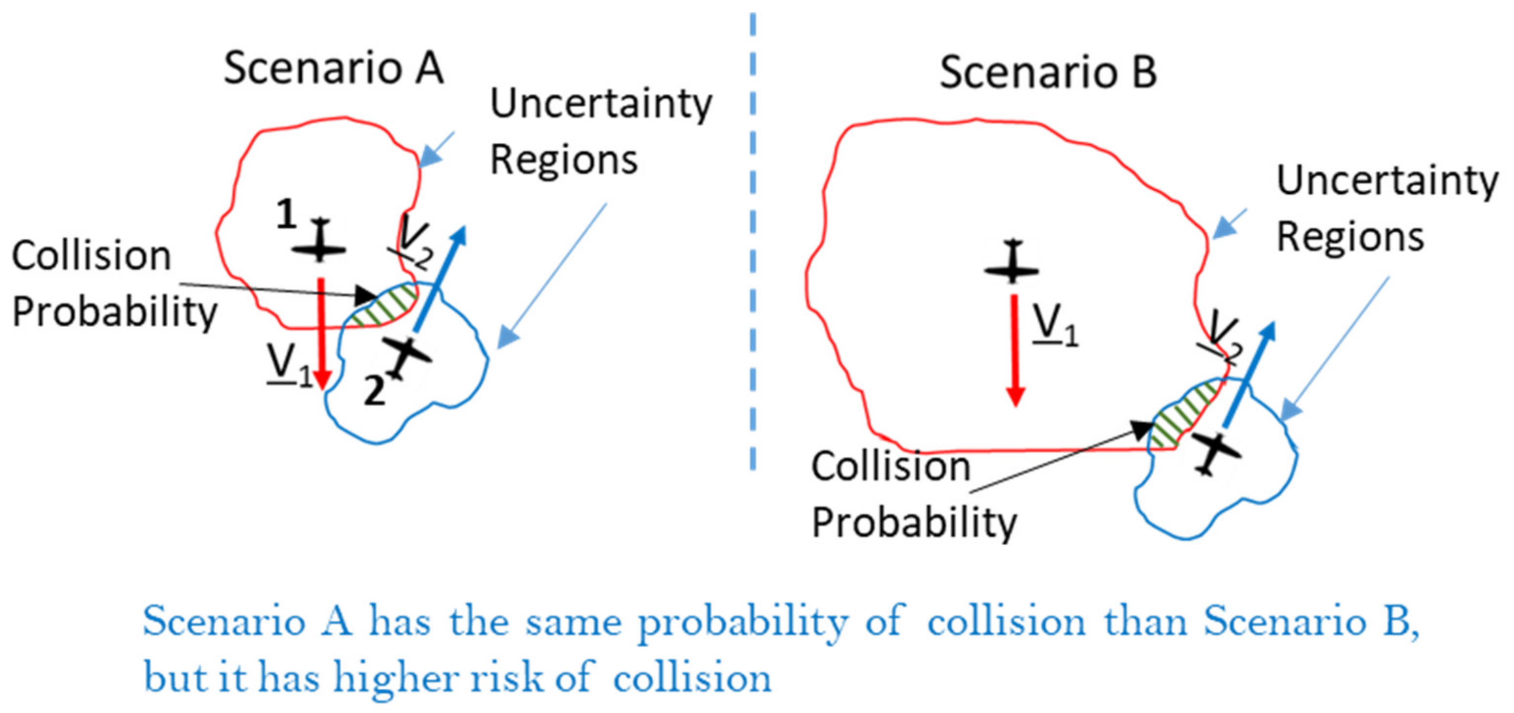
First, it can be easily verified that, when the predicted horizontal and vertical distances between ownship and intruder show very low accuracy, the probability of a collision over the time horizon T can be very low (and below the threshold ε) even if a specific intruder can be a potential collision threat. This situation is depicted in the Figure 5 where two intruders with different trajectory prediction accuracy have the same probability of collision if strictly computed using (3a).
In other terms, simply using the probability of collision would require that the threshold be variable with the accuracy of prediction (which is also variable along the predicted trajectories). To avoid this, the concept of Relative Probability (RPr) of collision as an index of the conflict threat level is introduced. The RPr is defined as the ratio between the maximum probability of collision with the current encounter geometry and the maximum probability that would be obtained in a perfect collision situation (i.e., when the distance to the Closest Point of Approach is predicted to be 0). In mathematical terms, given the following function of collision probability as a variable of time that shall be evaluated over the time horizon T:
P r d H t D     h t H = f P ( d H A t , h A t , σ t ) ,
where dHA and hA are, respectively, the average values of distance and relative altitude between the generic intruder and the ownship and σ their accuracy; the related maximum probability of collision over the time horizon T can be written as:
f P t ¯ = max t t k , t k + T f P d H t , h t , σ t ,
where t ¯ is the moment in time at which the collision probability has its maximum value. Then, using Equations (7) and (8), the RPr index for a given intruder encounter is defined as:
R P r = f P t ¯ f P 0 , 0 , σ t ¯
Considering the above definition, it can be easily verified that Scenario A of Figure 5 has a higher RPr than that of Scenario B, according to the evidence that the former poses a higher risk of collision between the two aircraft. Moreover, it can also be intuitively noted that the RPr is less sensitive to possible variations of the accuracy on distance and relative altitude, because this quantity is present in both the numerator and denominator of definition (9).
Anyway, RPr is still an index related to a single encounter or potential conflict with a surrounding fixed obstacle, while the proposed CDA algorithm needs to quantify the risk level associated to any possible hazard, also evaluating possible maneuvers.
To this aim, let us first note that the RPr index can only assume values in the compact set [0…1]. A small maneuver of either the ownship or the intruder is likely to produce only small variation in this value, so we can consider the RPr a continuous function of the ownship maneuvers. We recall here that, following the assumption of Section 5.1, the possible maneuvers that the ownship can perform are characterized by a single value (track angle or vertical velocity for the horizontal and vertical axes, respectively). Therefore, for each intruder or fixed obstacle, the RPr function can be evaluated on a suitable grid of ownship commands for each type of CA maneuver. The number of points on the grid is a tuning parameter and shall be determined based on the variability of the probability and on the resolution that is requested for the final velocity value. Verification of the RPr continuity with respect to ownship maneuvers shall be verified a posteriori with numerical simulations in different encounter scenarios, as well as by performing grid spacing tuning.
Now, let us evaluate, at a given time tk and for each intruder and path constraint ν in 1…N + M, all the maps R P r k v as a function of the own aircraft maneuvers y i j , where j = 1…4 is the type of maneuver (right turn, climb, etc.) and y i Y k with i = 1 Z j is the grid of ownship maneuvers for the j-th maneuver type. With these maps of relative probability, it is possible to compute the following four Overall Relative Probability (ORPr) functions:
O R P r k j y i j = max v   R P r k v y i j
The ORPr functions (one for each type of considered avoidance maneuver: left/right turn, climb/descend) includes almost all the information needed by the CDA algorithm for taking a decision and computing the optimal escape command, as will be described in the following sections. Actually, these functions give an estimation of the highest conflict risk level that is expected in the time horizon T in case the own aircraft either continues on the current flight path or performs a maneuver. In this sense, these functions almost completely characterize the current flight scenario and its possible evolutions, also giving detailed indications of where to go to lower the conflict risk.
The following section details the methods that can be used for estimating the relative probabilities for air traffic and the surrounding fixed obstacles, while the subsequent sections describe the computation of the optimal avoidance maneuver and the decision-making process.
Note that the above method for conflict risk level assessment does not prioritize intruders and/or fixed obstacles. All possible hazards are fairly treated, even if they are intrinsically prioritized because of the associated conflict risk level that, however, is not evidenced in the ORPr. This is in line with the philosophy of the proposed CDA algorithm, in which it is only important to understand if the own aircraft has currently, and would have future, safe maneuver margins for avoiding any conflict, no matter how many and which specific threats caused the conflict situation. On the other hand, it is possible to use the single RPr functions to identify the most hazardous threats, because they can be important to display to the remote pilot.

5.4. Estimation of the Conflict Risk Level for Each Hazard

The above method for assessing the conflict risk level associated to the current scenario and its evolution is based on the estimation of the RPr as function of the ownship maneuvers, for each intruder and obstacle from the surrounding environment. The proposed methods for such estimation are described below.

5.4.1. Air Traffic

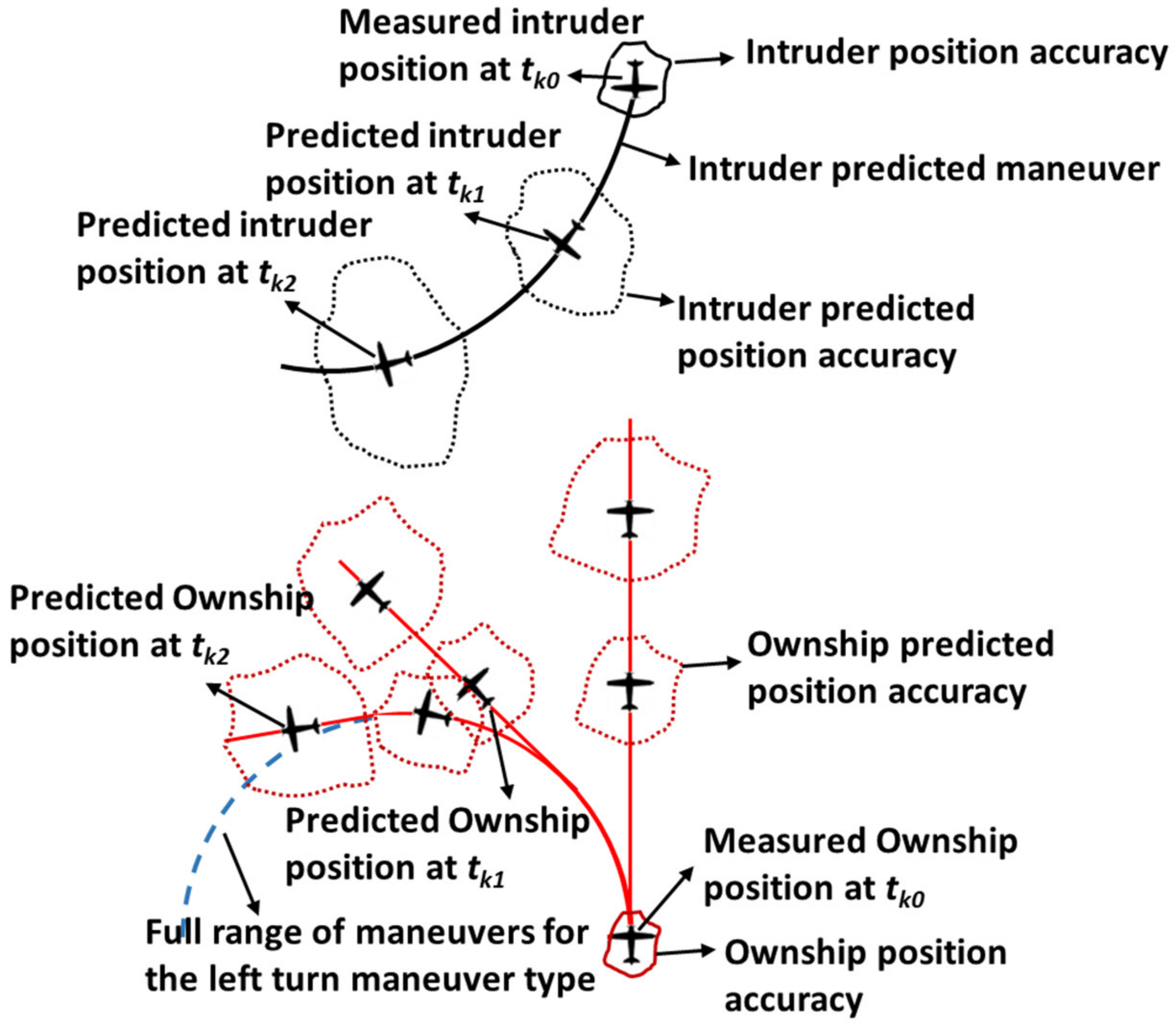
Concerning the air traffic, evaluation of the RPr functions to be used for Equation (10) is performed by first setting a given maneuver step according to the chosen fixed grid and then predicting the ownship trajectory, as depicted in the Figure 6.
After that, using the predicted trajectories and related accuracies, Equation (7) is evaluated. To this end, several techniques can be used, such as the one proposed in [18]. However, in this context a different method is adopted in order to reduce the computational effort at the cost of accepting some errors in estimating the relative probability.
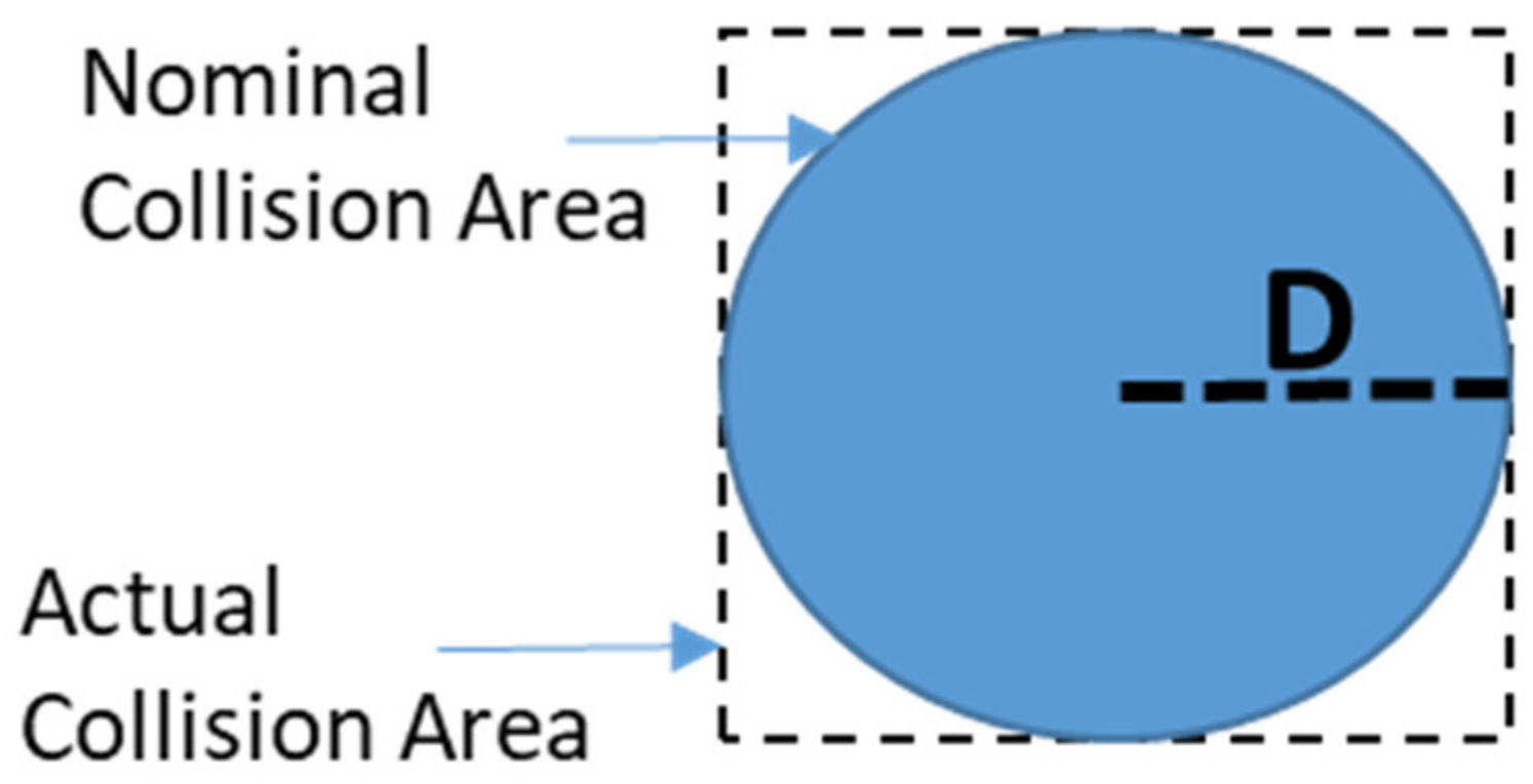
Specifically, the RPr is computed approximating the NMAC cylindrical volume with a right parallelogram prism (Figure 7) and assuming that relative position coordinates between ownship and intruder ( P x r e l , P y r e l , P h r e l ) are independent stochastic variables with time-uncorrelated Gaussian distribution.
The above assumption lets us write the probability of collision ( f P k ) as follows, for any t in the look-ahead interval T.
f P k = P r d H t D h t H P r ( P x r e l t D · P r P y r e l t D · P r P h r e l t H ,
The probability of each Gaussian variable, namely P x r e l , P y r e l , P h r e l , of being less than the associated dimension of the NMAC volume is evaluated through an analytical approximation of the standard normal cumulative distribution function defined in [19].
In this way, the RPr for each intruder can be estimated as follows:
R P r k ζ y i j f P k ζ Δ P k r e l ( y i j , t C P A ) , σ ( y i j , t C P A ) f P k ζ 0 , σ ( y i j , t C P A )
where ζ is the subset of intruders inside the ν hazard set, t C P A is the time to closest point of approach [5] and Δ P k r e l y i j , t C P A and σ y i j , t C P A are the current relative position prediction and the current prediction error, respectively, for the y i j ownship maneuver evaluated at t C P A .
The method above for computing RPr functions is relatively simple in that it only needs the evaluation of the ownship and intruders’ trajectories prediction with related errors and tCPA, for which several methods exist in the literature [5,6,13] that can also be expressed with explicit analytical relations. On the other hand, in case cartesian relative positions cannot be used (such as in the case of relative positions in polar or cylindrical coordinates) it is possible to find a different approximation of the NMAC volume so to be again in similar conditions as requested by Equations (11) and (12). Moreover, some correlation exists between the horizontal and vertical coordinates, Equation (11) can be considered as a worst case, as this correlation is neglected in the computation.
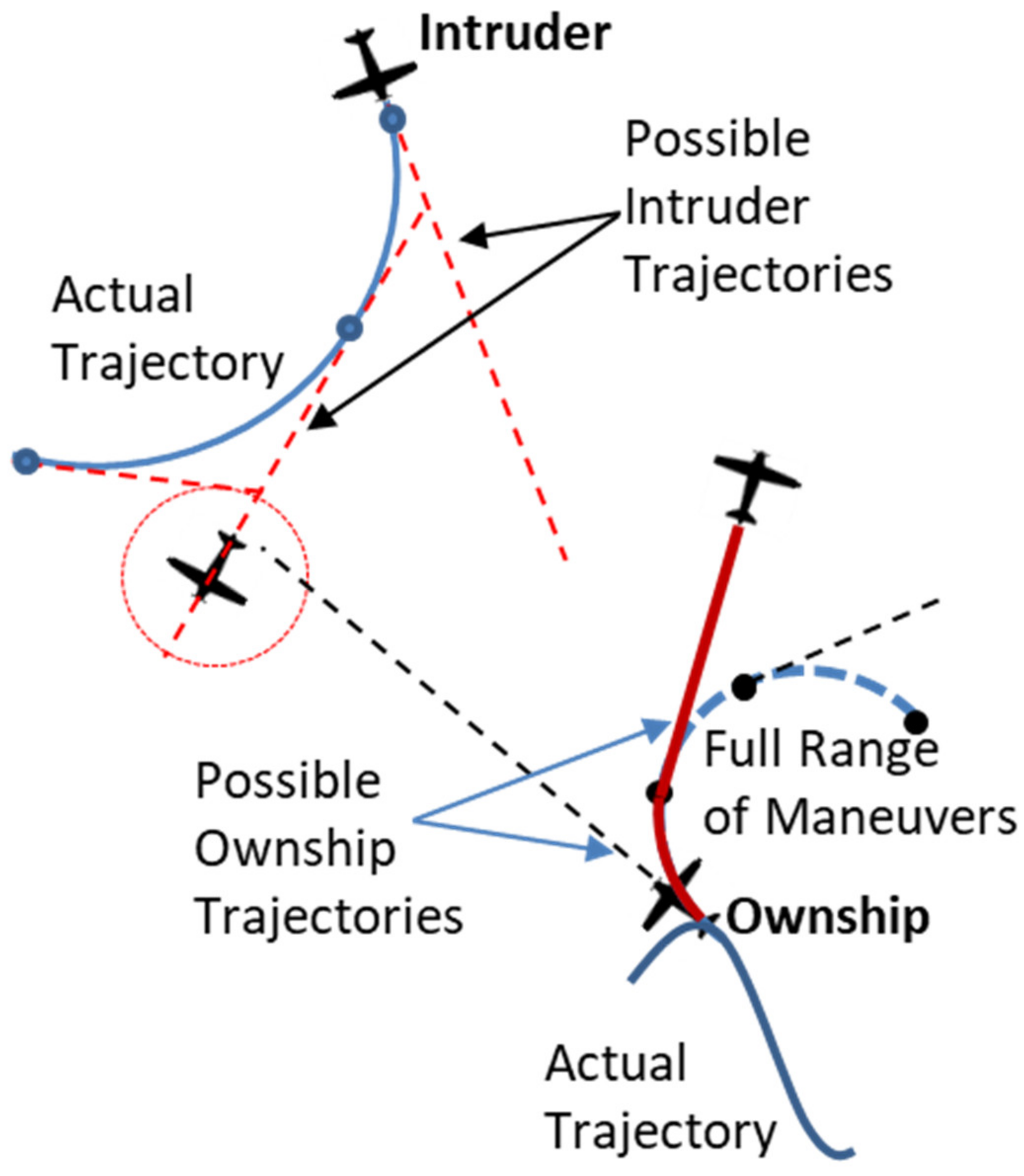
When the intruder is turning (as identified from the flight mode), the RPr is computed by choosing the worst value between a set of trajectories that considers the intruder can stop its turn maneuver and go straight, as shown in the Figure 8. The number of points along the intruder’s turn trajectory that are used for such assessment is an algorithm tuning parameter (the default is five points). This different way of computing RPr for turning intruders takes into account the uncertainty in the intruder prediction trajectory.

5.4.2. Surrounding Areas and Obstacles

These hazards have very different (known) shapes from the NMAC volume, do not move (or their movements can be neglected in the timeframe of the avoidance maneuver) and typically their position is known quite accurately. Moreover, it should be pointed out that the CDA algorithm is not used for avoiding fixed obstacles, because this is a task of other on-board systems (e.g., the Terrain Avoidance and Awareness System). Therefore, a potential conflict with fixed obstacles only would not start any avoidance maneuver, unless air traffic is also involved. In this case, the air traffic avoidance maneuver accounts for these path constraints. Finally, the computation considering generic path constraints usually requires high computational effort, so it should be as simple as possible.
These differences with air traffic lead to the conclusion that the above method is not fully suitable for RPr computation in this case. Nevertheless, evaluation of RPr as a function of ownship maneuvers can still be performed using the same procedure above described, i.e., using a grid in the ownship possible maneuvers and computing the RPr for fixed obstacles on the resulted predicted trajectory.
Based on the above, the proposed algorithm assumes the following simple relation for surrounding areas and obstacles:
R P r k γ y i j = 1 ,       i f   P A y i j   i n t e r s e c t   t h e   o b s t a c l e   i n   t k ,   t k + a · T 0 ,   i f   P A y i j   d o   n o t   i n t e r s e c t   t h e   o b s t a c l e   i n   t k ,   t k + a · T .
where γ is the subset of the fixed obstacles within the ν hazard set and P A y i j is the ownship trajectory that resulted from applying a potential collision avoidance maneuver.
Equation (13) assumes that RPr can assume only two values: a maximum and a minimum probability, here valued one and zero, respectively. Adopting only two values allows computation of the RPr by evaluating geometrical intersections between boundaries of the fixed obstacles and the ownship trajectory, with an affordable computational effort. In this respect, it can be argued that this method could over-simplify the problem with a resulting low accuracy. Indeed, because the position and shape of fixed obstacles and the ownship’s trajectory are typically known with good accuracy, it can be easily verified that the collision probability with a fixed obstacle changes very rapidly from zero to one so the approximation of Equation (13) can be considered adequate for our scope. On the other hand, increasing the size of fixed obstacles with a suitable safety margin can conservatively account for the current navigation total system error of the ownship and accuracy of the position and shape of the obstacle.
Note that using one as the maximum value of the RPr implies that these hazards are always assumed as ‘hard’ path constraints, i.e., the vehicle is not allowed to enter the related forbidden areas. Anyway, in case ‘soft’ path constraints are enforced (such as bad weather areas that can be entered for some time/distance assuming a certain risk), a risk level lower than one can be specified in the Equation (13) to account for this possibility.
Finally, the parameter a ≥ 1 in Equation (13) specifies that RPr for fixed obstacles is performed over a time horizon equal to or greater than the one used for air traffic. Actually, this parameter is set to one when computing the ORPr functions used for deciding whether an avoidance maneuver is needed and is above one (and typically equal to two) when computing the optimal maneuver. This allows enough clearance from any obstacle to avoid alerts from other safety modules (such as Terrain Awareness Systems) and easing the return back to the original flight path after the conflict has been resolved.
In order to evaluate the geometrical intersections between the ownship trajectory and the obstacle, a dedicated computation procedure is implemented depending on the shape of the obstacle or area [20]. Note that this procedure is also used to evaluate the time instant at which the intersection is detected so as to easily compute RPr in both T and a·T intervals. In detail, let us denote the predicted position of the ownship vehicle in the North-East-Up (NEU) reference frame along the i-th maneuver of the j-th type as follows:
P A m j , i = P A m N j , i ,   P A m E j , i   , P A m U j , i .
The following methods can be used for the types of surrounding obstacles considered in this paper.

Terrain

With reference to the terrain, Equation (15) guarantees that the trajectory altitude is always greater than the local elevation data provided by the function H( P A m E j , i , P A m N j , i ).
P A m U j , i >   H ( P A m E j , i ,   P A m N j , i ) .
In other terms, given the predicted trajectory of the ownship with a specific maneuver, the problem is simply to interrogate a terrain elevation database for checking that altitude of the aircraft is above the terrain elevation on the given trajectory. In this implementation, the Digital Terrain Elevation Data (DTED) Level 1 is used for modelling the terrain elevation map. Nevertheless, other terrain elevation databases can be used. Moreover, the availability of an elevation database of an urban area would also allow consideration of the presence of buildings and other similar obstacles so as to support Urban Air Mobility applications.

Cylindrical Forbidden Area

Given xs, ys, rs, hs and Hs are the East and North positions of the center, the radius, the starting height and the ending height, respectively, of the s-th cylindrical forbidden area, the following equation defines such constraints:
r s 2 P A m E j , i x s 2 P A m N j , i y s 2 0 w h e n :   h s P A m U j , i H s ,   s = 1 , S
Equation (16) expresses that the ownship horizontal path does not intersect the cylindrical area, while the vehicle altitude is within the height interval of the forbidden area.

Right Prismatic Forbidden Area

Assuming that xl,m, yl,m are the East and North positions of the m-th vertex and hl, Hl the initial and final altitudes, respectively, of the l-th right prismatic forbidden area, the following relations define the condition for non-intersection these constraints.
y l , m o d m + 1 , M l y l , m x l , m o d m + 1 , M l x l , m P A m E j , i x l , m + y l , m P A m N j , i > 0   w h e n : x l , m o d m + 1 , M l P A m E j , i + x l , m P A m E j , i x l , m o d m + 1 , M l x l , m h l P A m U j , i H l   l = 1 , L   a n d     m = 1 , M l
where the function mod(a,b) provides the remainder after division of a by b.
Equation (17) simply expresses that the ownship horizontal path does not intersect any side of the right prismatic area, while the vehicle altitude is within the height interval of the forbidden area.

Area of Operation

With reference to the area of operation (not limited in height), assuming that xp and yp are the East and North positions of the p-th vertex of the area of operations, (18) expresses the non-intersecting constraints in this case.
y m o d p + 1 , P y p x m o d p + 1 , P x p P A m E j , i x p + y p P A m N j , i > 0   w h e n x m o d p + 1 , P P A m E j , i + x p P A m E j , i x m o d p + 1 , p x p   p = 1 , P
The above methods deal only with some limited shapes. This is not limiting because more general obstacle shapes can be either obtained by merging the above ones or derived from more complex data using some dedicated software modules. For instance, bad weather areas can be included using one of the above shapes provided by dedicated software that evaluates the level of the hazard of the surrounding areas based on the available meteorological information and some processing [21].

5.5. Computation of the Optimal Avoidance Maneuver

As mentioned, the ORPr functions in Equation (10) return the level of collision risk for each type of maneuver (left/right turn, climb/descend) in a pre-fixed grid of the possible commands (i.e., the track angle for the horizontal plane and the vertical rate for the other axis).
Therefore, for each type of ownship maneuver, the minimum value of this ORPr gives the velocity change that shall be required to minimize the conflict risk level:
y o p t k j = min i O R P r k j y i j .
Then, the optimal collision avoidance maneuver yoptk can finally be chosen as the one that leads to the minimum conflict risk level and, in case of equal risks, the minimum change of the own aircraft nominal velocity among the four possible maneuver types, according to Equation (3). Note that, as pointed out in the previous sub-section, the ORPr functions to be used in Equation (19) shall consider an extended time horizon a·T for fixed obstacles. With this optimal maneuver, avoidance of a conflict is guaranteed (under a probabilistic sense) only if the value assumed in the minimum point is below the thresholds on the RPr that translate the constraints of the original problem (3).
In this way, the original CDA problem (3) is solved including constraints (3a) and (3b) in the cost function, with the remaining constraints enforced by the assumptions of Section 5.1 and intruder track processing described in Section 5.2. Finally, note that the solution can be found executing only (N + M) · ΣjZj evaluations of the RPr so obtaining a polynomial computational complexity that increases with the number of maneuver grid points, intruders and fixed obstacles.

5.6. Decision Making Process

Having computed the optimal avoidance commands and the ORPr functions that describe the conflict risk level related to the current scenario and its possible evolutions, a decision is taken whether a collision alarm should be issued and which of the four optimal avoidance commands should be automatically executed. Before describing the proposed solution, it is necessary to compute two simple indexes that would easily support this decision-making process, no matter how many intruders or fixed obstacles are being considered and which one of these actually poses the major risk of conflict.
The first index, named Margin of Maneuver (MM), is defined as the ratio between the range of possible avoidance maneuvers and the full maneuver range given by the current ownship flight envelope limits. This index indicates whether the current situation is safe, i.e., the own aircraft has sufficient possibilities of performing some escape maneuvers. MM can be written as:
M M k = I k j Y k   ,
where I k j is the set of possible resolution maneuvers and Yk is the full set of available maneuvers at tk. Having discretized the range of possible maneuvers, Equation (20) can simply be computed as the ratio between the number of commands that have an ORPr below a given safety threshold and the number of all possible commands in any axis. In this case, the ORPr functions for fixed obstacles are evaluated over the same time horizon T of air traffic, differently from the ORPr used in Equation (19).
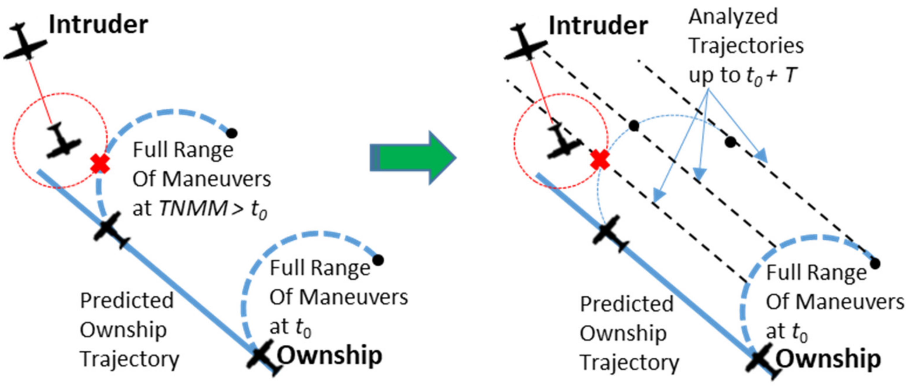
The second index, named the Time to Null Maneuver Margin (TNMM) tells how much time is remaining until the situation becomes so bad that there will be no possibility of performing an escape maneuver (i.e., the MM is nulled). In other terms:
T N M M k = t k j ¯ ,           j ¯ : M M j ¯ = 0   for   j = t k t k + T .
Note that the TNMM is computed considering only air traffic. This is in line with the assumption that the CDA system only aims to avoid air traffic accounting for fixed obstacles, to be managed by other on-board systems. Evaluation of Equation (21) is performed by first considering each single intruder and then combining these evaluations to estimate an overall TNMM value.
Considering single intruders, let us first note that TNMM is related to the instant in which no more commands are possible for all maneuver types under consideration. Therefore, the evaluation should be performed for each type of maneuver and then the maximum time chosen. Two different methods are used for the horizontal and vertical axes. In Figure 9, the procedure adopted for the evaluation of TNMM in the horizontal plane is reported.
The TNMM for horizontal maneuvers should be computed by predicting the intruder and own aircraft trajectories (here considered to be straight) and then checking that all the maneuvers do not have an RPr below the given safe threshold, at any time in the considered interval T (see Figure 9, left). Instead of this straightforward but computationally intensive method, the evaluation is operated by first performing the maneuver and then finding the time instant at which a straight trajectory will have an RPr below the threshold (see Figure 9, right). This is more computationally efficient because there is an analytical solution for evaluating Equation (12) in the straight trajectory segments.
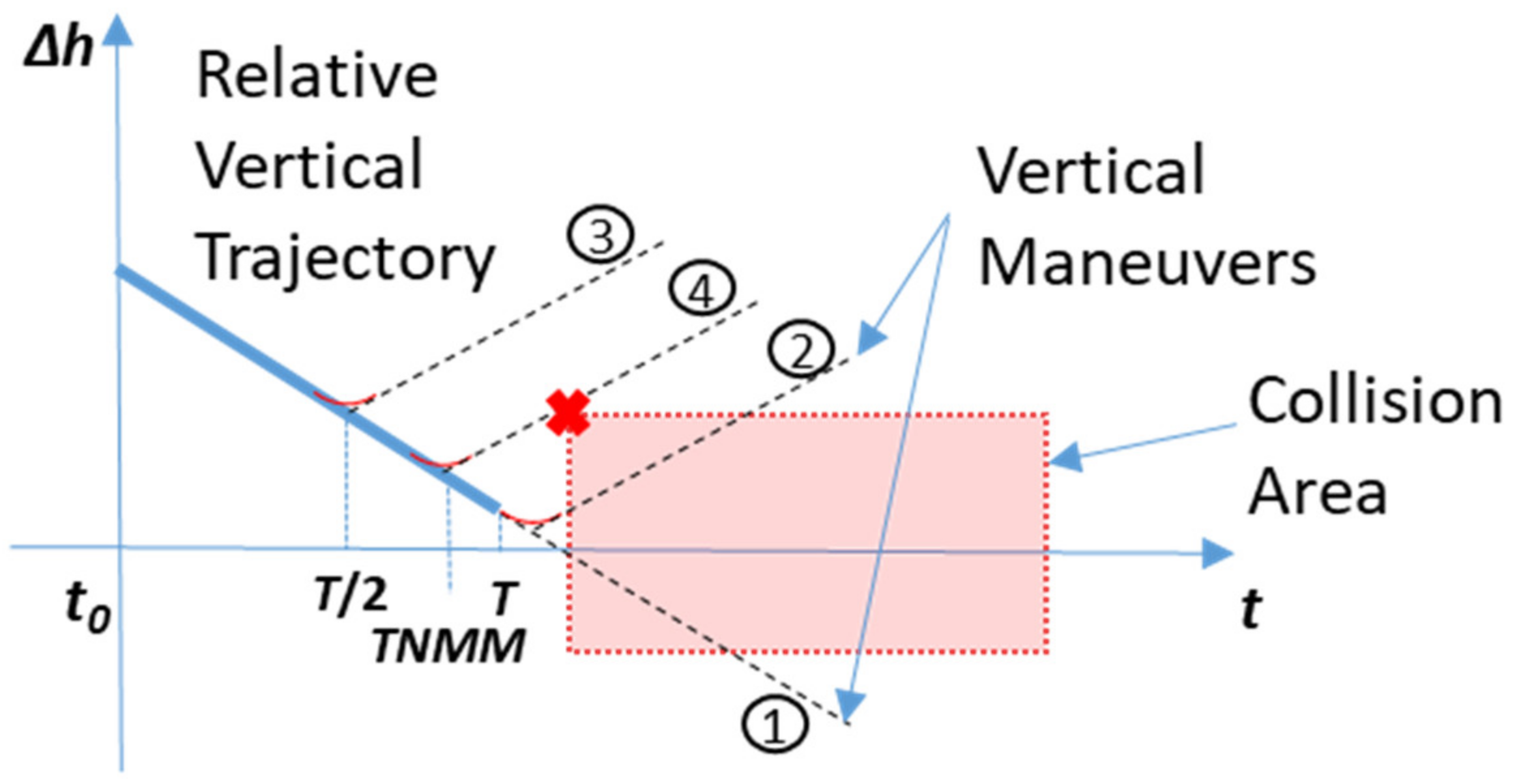
TNMM for vertical maneuvers can be estimated with an iterative process that considers the relative altitude variation and a constant (worst case) on set time (see Section 5.1). The process is depicted in Figure 10, where a finite number of RPr evaluations are performed using a bisection search technique.
After the evaluation of TNMM for each single intruder, the combined overall TNMM can be computed as follows:
T N M M k = M M k i ¯ M M k · min T N M M k i ,
where i is the index in the set 1…N intruders and i ¯ is the index associated to the minimum value of the TNMM computed for a single intruder. Equation (22) relates the single intruder’s TNMMs to the overall TNMM at tk. Indeed, using the ratio between the MM of the worst intruder and the global MM is a way to take into account how much the other intruders (and fixed obstacles) contribute to reducing the final TNMM. Indeed, finding the TNMM when more than one threat is contributing to the MM reduction is a tricky problem that can be very computationally intensive. Relations different from Equation (22) or other methods can be adopted, given that they are computationally affordable and prove to be sufficiently accurate. To overcome this major limitation of the algorithm, some future improvements could include using artificial intelligence techniques directly on the ORPr functions so as to predict the possible scenario evolution based on experience, as humans normally do.
Having computed MM and 
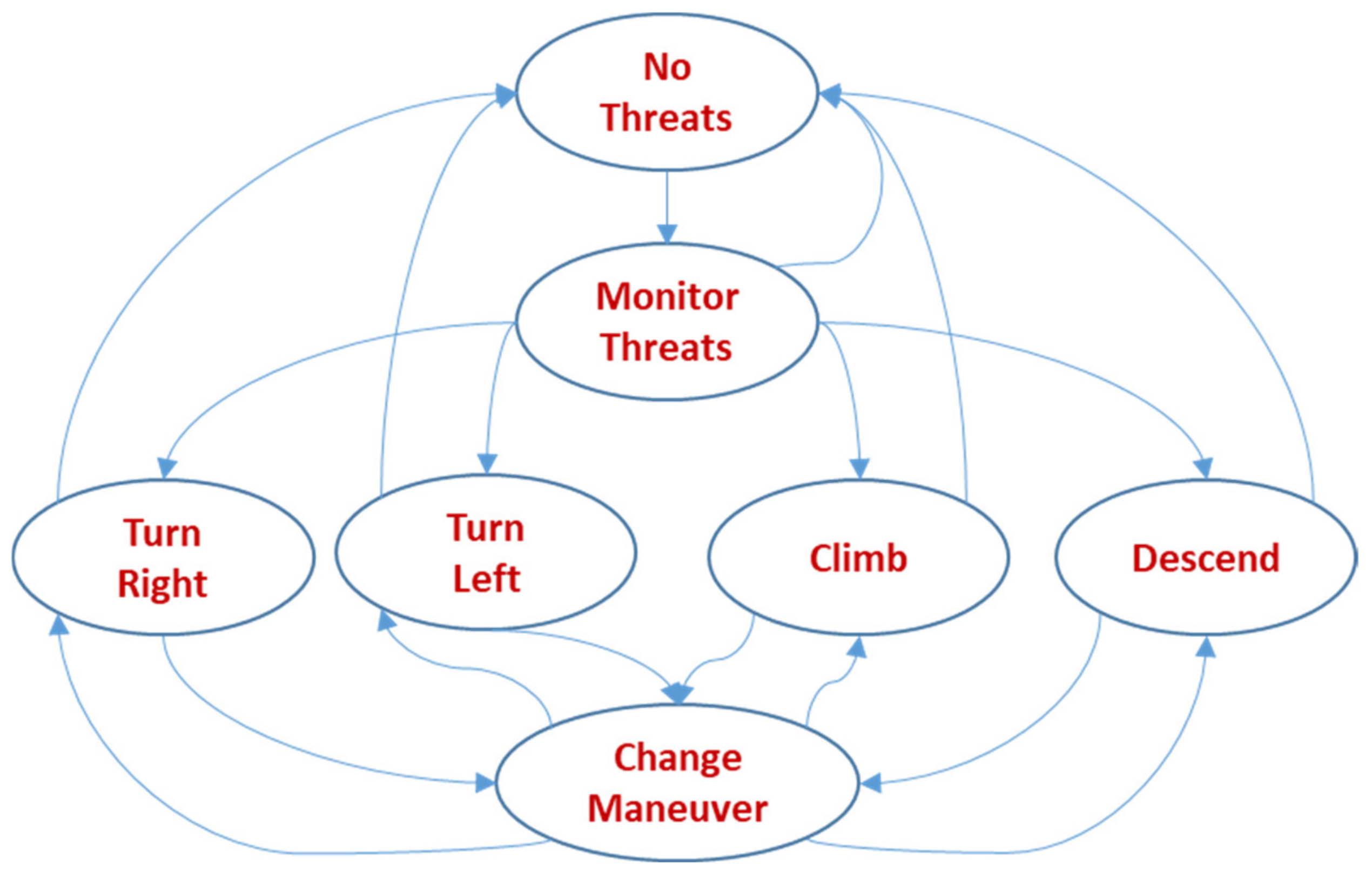
TNMM at the current time step, we have all the elements necessary to take an automatic decision. The proposed decision-making process is basically implemented as a discrete state machine with heuristic rules for state transitions (see Figure 11).
The states and transitions in such decision making logic are as follows:
  • No Threats corresponds to no imminent potential collision.
  • Monitor Threats indicates that at least one potential collision is detected, not considering any maneuver (i.e., the RPr is below the threshold for the predicted intruder and ownship trajectories). This is a pre-alert status that is basically introduced to inform the pilot through the ground station display that a potential conflict has been detected.
  • Turn Right/Left, Climb, Descend correspond to raising a collision warning alert and executing the respective maneuver. Only one of these states is accessed when MM or TNMM is below given thresholds (to be tuned). The type of avoidance maneuver is selected after performing several considerations, as better described below. During the maneuver execution, and until a safe situation is restored, the algorithm continuously evaluates the situation to check whether the current avoidance maneuver is still safe.
  • Change Maneuver is accessed if the current avoidance maneuver type is no longer safe, and a revision of the current maneuver type or command is required.
The process of selecting the type of maneuver and the related command considers the safety of flight, TCAS-II interoperability and Right of Way (RoW) rules, as specified in Section 2. Therefore, the optimal command computed as per Section 5.5 is not always used.
When considering multi-intruder scenarios, the most hazardous intruder is selected to comply with TCAS-II interoperability and RoW rules. This intruder is chosen using the following criteria:
(a)
Presence of a TCAS-II Resolution Advisory from the intruder;
(b)
Number of maneuver types with a null margin of maneuver;
(c)
Lower time to a null margin of maneuver;
(d)
Lower margin of the maneuver.
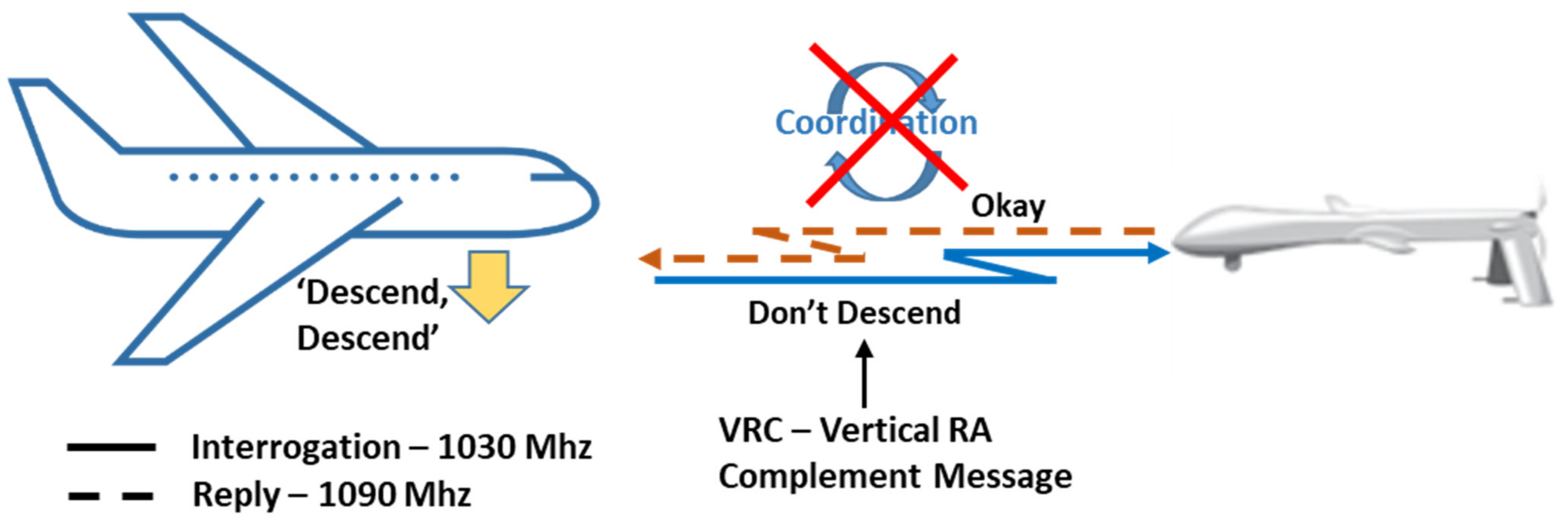
The TCAS-II interoperability implementation is based on the so-called Responsive Coordination. Actually, when an intruder is identified as TCAS-II-equipped, the proposed CDA algorithm complies with the Vertical Resolution Advisory Complement (VRC) provided by the other aircraft [12], if this has been received from the on-board sensors (see Figure 12).
In case no VRC has been received or for aircraft not equipped with TCAS-II aircraft, the RoW rules are basically applied using quantitative criteria (with different thresholds), as specified by DAA MOPS, App. H [5]. The maneuver type suggested by the RoW rules is selected only if it is not detrimental to safety, i.e., the predicted risk level associated to its optimal command is as low as other possible maneuver types.
Otherwise, or when the ownship has RoW, the maneuver type and the related optimal command are chosen as computed in Equation (19).

6. Tuning and Numerical Assessment

Before performing a numerical assessment of the proposed CDA algorithm, a parameter tuning process is performed using Fast Time simulations. The simulator environment is schematically shown in Figure 13.
The simulator comprises, other than the CDA algorithm under test, a generator of air traffic trajectories, the surveillance and navigation error models, the data related to the fixed obstacles in the surrounding environment and the 6DoF simulation model of the unmanned aircraft with its related autopilot. The simulator includes a complete DAA algorithm, integrating a Remain Well Clear (RWC) module (see Section 1) with the proposed CDA algorithm. The aim of the RWC module [5,6,22] is to provide air traffic situational awareness to the remote pilot, so mitigating the number of NMAC events.
Using this simulator, the tuning of the thresholds for RPr, MM, TNMM is performed using several air traffic scenarios and trajectories mainly extracted from the DO-317B test tracks [23]. These test tracks account for real scenarios in different airspaces (controlled classes A to C and not controlled classes D to G) and in terminal areas close to airport and during approach and take-off procedures. The optimal parameter set is found by minimizing the number of NMAC events in the performed simulations, also taking into account the RWC alert timing [5,6,22]. In other terms, the CDA thresholds are tuned in order to avoid overlapping with the RWC caution alerts, while ensuring that NMAC are avoided.
The own aircraft was modelled as a fixed wing Tactical Unmanned Vehicle with an air speed up to 100 knots, a climb/descent rate of about 1000 fpm, a 40 deg maximum bank and an altitude ceiling of up to 12,000 ft. On the other hand, different intruder types were used: very light aircraft, general aviation, business jets and airliners.
The intruder aircraft are considered cooperative and equipped with a Mode S-ES transponder (i.e., ADS-B Out) working in the standard frequency of 1090 Mhz. This sensor is characterized by two levels of measurement errors for air traffic surveillance:
  • Highly accurate, characterized by intruder position and errors modelled by a null mean and a standard deviation of [10 10 15] m [5 5 5] m/s, respectively;
  • Medium accuracy, characterized by intruder position and errors modelled by a null mean and a standard deviation of [20 20 30] m [8 8 8] m/s, respectively.
Regarding ownship navigation errors, they were set as gaussian distributed with null mean and standard deviation of [6 6 6] m for position and of [3 3 3] m/s for velocity (typical performance of GPS receivers).
Several different conflict geometries were simulated in levelled or during climb/descend flights, such as: head-on encounters with lateral displacements, lateral convergence at low and high speed, overtaking at low and high speed, etc. The encounters were selected with the objective of assessing the robustness of the CDA algorithm in avoiding the collision and minimizing nuisance alerts, as also occurs in multi-intruder and maneuvering scenarios.
These simulated air traffic scenarios are representative of future situations in which unmanned and manned aircraft perform their missions at mid/low altitudes in the civil airspace where several constraints can be present, such as terrain, bad weather and no-fly zones. For instance, setting up no-fly zones could allow considering one or more small, unmanned vehicles that are performing operations in a given area of the unmanned traffic management (UTM) airspace at very low-level altitudes below 500 ft.
Once the optimal parameter was set, the CDA algorithm was stress tested in more challenging scenarios in order to assess its performance with respect to other CDA algorithms. These scenarios include encounters during the landing or taking off phases with the presence of fixed obstacles (terrain, no-fly zones) and geo-fencing constraints. Two simulation examples of such scenarios are described below.
In the first scenario in airspace class G, the ownship (a Tactical Unmanned vehicle) is taking-off while the intruder (a General Aviation aircraft) is landing on the same airport in presence of a no-fly zone positioned on the right side of the ownship direction of flight (Figure 14a). During the encounter, both aircraft are moving with an absolute vertical speed of 5 m/s and a ground speed of 45 m/s.
In this situation the proposed CDA algorithm, after collision alarm activation, proposes an avoidance maneuver to the remote pilot, giving them five seconds to abort its automatic execution. In the analyzed case, the proposed maneuver is automatically executed (Figure 14a) considering the geometry of the encounter, the no-fly zone, and the terrain.
The optimal maneuver is executed at a horizontal distance between the aircraft of about 3000 m with a closing speed of 90 m/s. At the minimum horizontal distance, the conflicting aircraft are at about 1010 m, therefore widely outside the NMAC volume. The RPr for the four optimal avoidance maneuvers at each time step are depicted in Figure 14b. During the climbing phase the RPr of the right turn and climb maneuvers are equal to one due to the no-fly zone and the descending intruder, respectively. After a few seconds, when the ownship is above a minimum height threshold, the terrain constraint is accounted for by the CDA algorithm that sets the RPr of the descend maneuver to one. At 19 s, when the ownship is at an altitude of about 310 m, the RPr of the descend maneuver becomes zero. This indicates that there is an optimal descend maneuver that allows avoidance of the intruder and the terrain (the latter evaluated with a look ahead time of 2 × 30 s). At 21 s, the descend RPr starts increasing again due to the reduced distance from the intruder. On the other hand, the RPr of the optimal left turn maneuver is always equal to zero with better values of MM and TNMM determining its automatic execution at 27 s. When the avoidance maneuver ends, all the RPr values move to zero as shown in Figure 14b.
In a different scenario, a head-on encounter between a Tactical UAV and a business jet in airspace class D is simulated, during a level flight close to the boundaries of the area of operation with a no-fly zone on the left of the ownship direction. During the encounter, the ownship and the intruder have groundspeeds of 50 m/s and 150 m/s, respectively.
The proposed maneuver is automatically executed at a horizontal distance between the aircraft of about 6500 m with a closing speed of 200 m/s (see Figure 15a). At the minimum horizontal distance, the conflicting aircraft are at about 2560 m, and therefore are widely outside the NMAC volume.
Figure 15b shows the behavior of the RPr for the four optimal avoidance maneuvers. The RPr of the left turn maneuver rapidly saturates to one due to the no-fly zone, while the RPr of the climb and descend maneuvers first starts increasing, due to the intruder relative distance, and then steps to one because the border of operation’s area is approaching. The RPr of the optimal right maneuver is always zero, determining its execution at 76 s.

7. Real Time Validation

In order to verify that the proposed CDA algorithm can be executed in real time and to assess human pilot judgment about its behavior, a prototype software was implemented and then integrated in a detailed HW-in-the-Loop real time simulator of a tactical unmanned aircraft. The unmanned simulator is part of a real-time simulation facility where experimental tests can be performed with the presence of expert pilots and air traffic controllers. The real time facility used for the subject validation of the CDA algorithm involved:
  • An HW-in-the-loop real-time simulator of a tactical RPAS;
  • A simulation scenario generating the air traffic and the conflicting intruder together with other agents of the scenario such as: weather hazards, no-fly zones, navaids and GPS time and satellite constellations;
  • A pseudo-pilot station for on-line modification of the traffic trajectories generated by the scenario simulator, based on air traffic controller instructions;
  • An emulator of a controller working position implementing the advanced functionalities needed to support the controller in its air traffic monitoring and control tasks.
The real time implementation of the proposed CDA algorithm comprises the development of a dedicated display in the ground control station, named the Cockpit Display of Traffic Information (CDTI). The CDTI basically displays the air traffic to the remote pilot with different colors based on the associated conflict risk level. Moreover, it displays the Conflict Bands that are the maneuvers to be avoided because they can cause a conflict and the avoidance maneuvers suggested by the CDA algorithm. The conflict bands generated by the CDA algorithm are obtained by applying a suitable threshold to the ORPr functions and are shown in red.
Several real time validation tests were performed to assess the capability of the proposed CDA algorithm to also behave correctly in case of complex encounter scenarios. In this paper, we describe only one of the performed tests to demonstrate the ability of the proposed CDA algorithm to solve complex conflict situations.
The sample simulated scenario foresees a level head-on encounter in the airspace class G between a fixed wing tactical unmanned aircraft (see Section 6 for its performances) flying under the Instrumental Flight Rules (IFR) and a cooperative General Aviation manned aircraft flying under Visual Flight Rules (VFR), equipped with an ADS-B OUT transponder without TCAS-II. The encounter was located close to a no-fly zone placed on the right side of the unmanned aircraft flight plan (Figure 16a). In this situation, the air traffic controller provides only flight information, leaving the conflict resolution responsibility to the remote and manned pilots.
During the conflict, the DAA system first shows to the remote pilot the presence of the no-fly zone (red box in Figure 16a) on the right of the own aircraft by displaying a red band (see Figure 16b) that indicates not to turn right.
Then, while the flight of both aircraft continues with the intruder moving closer to the own aircraft, the DAA system first activates the RWC alerts (orange colored) and then the collision alert (Figure 17a). The situation evolves up to the activation of the automatic maneuver (Figure 18) that performs a left turn avoiding the NMAC volume with a resulting minimum horizontal distance of 600 m (Figure 19).
At the end of the collision avoidance maneuver, the unmanned aircraft is still in a loss of well-clear condition without any possibility of its recovery due to the low relative distance with respect to the intruder (orange conflict bands in Figure 17b).
This scenario also shows that, due to the presence of the no-fly zone, the CDA algorithm executes a left turn that is contrary to the RoW rules that would require a right turn.

8. Conclusions

This paper merges and extends the results of [14,15], providing a comprehensive and detailed description of a Collision Detection and Avoidance algorithm that is able to cope with complex conflict situations in the presence of multiple intruders, terrain, no-fly zones, fixed obstacles and bad weather areas. Moreover, the tuning process and the numerical assessment performed with a fast-time detailed simulator is also described by reporting some simulation results. Finally, the real time implementation of the proposed algorithm is demonstrated by performing HW-in-Loop and Human-in-the-Loop tests in a laboratory test facility.
Further work will expand the algorithm capabilities by using a suite of cooperative and non-cooperative sensors and will exploit machine learning and/or deep learning techniques to replace the current decision logic state machine with an artificial intelligence module to manage even more complex scenarios characterized by several interacting multi-intruder conflicts and path constraints.

Author Contributions

Conceptualization F.C.; software F.C., G.C. (Gianluca Corraro), G.C. (Giovanni Cuciniello) and L.G.; validation G.C. (Gianluca Corraro) and L.G.; writing—original draft preparation F.C. and G.C. (Gianluca Corraro); writing—review and editing G.C. (Giovanni Cuciniello) and L.G. All authors have read and agreed to the published version of the manuscript.

Funding

This research was funded by Italian Ministry of Research within the Italian National Aerospace Research Program (PRORA) managed by CIRA S.c.P.A., project TECVOL-II.

Conflicts of Interest

The authors declare no conflict of interest.

Acronyms

3DOF3 Degree-of-Freedom
6DOF6 Degree-of Freedom
ACAS-XAirborne Collision Avoidance System—X
ADAPTAdvanced Detect and Avoid ProTotype
ADS-BAutomatic Dependent Surveillance—B
CACollision Avoidance
CDACollision Detection and Avoidance
CDTICockpit Display of Traffic Information
CIRAItalian Aerospace Research Center
CPAClosest Point of Approach
DADetect and Avoid
DCPADistance at the Closest Point of Approach
DTEDDigital Terrain Elevation Data
EUDAASEUropean Detect And Avoid System (the project)
EUROCAEEuropean Organisation for Civil Aviation Equipment
FAAFederal Aviation Administration
FMSFlight Management System
GPSGlobal Positioning System
HWHardware
ICAOInternational Civil Aviation Organization
IFRInstrumental Flight Rules
LATLook-Ahead Time
MDPMarkov Decision Process
MIDCASMID Air Collision Avoidance System
MMMargin of Maneuver
MOPSMinimum Operational Performance Standards
NASANational Aeronautics and Space Administration
NEUNorth-East-Up
NMNautical Mile
NMACNear Mid Air Collision
NPNon-Polynomial
ORPrOverall Relative Probability
OSEDOperational Services and Environment Description
RoWRight of Way
RPASRemotely Piloted Aircraft Systems
RPrRelative Probability
RTCARadio Technical Commission for Aeronautics
TASTrue Air Speed
TCAS-IITraffic Collision Avoidance System—II
TNMMTime to Null Maneuver Margin
UASUnmanned Aerial Vehicle
USAUnited States of America
UTMUnmanned Traffic management
VFRVisual Flight Rules
VRCVertical Resolution Advisory Complement

References

  1. ICAO. Global Air Traffic Management Operational Concept, 1st ed.; ICAO: Montreal, QC, Canada, 2005. [Google Scholar]
  2. Consiglio, M.; Chamberlain, J.; Muñoz, C.; Hoffler, K. Concepts of integration for UAS operations in the NAS. In Proceedings of the 28th Congress of the International Council of the Aeronautical Sciences, Brisbane, Australia, 23 September 2012. [Google Scholar]
  3. Cary, L.; Coyne, J. ICAO Unmanned Aircraft Systems (UAS), Circular 328. In 2011–2012 UAS Yearbook—UAS: The Global Perspective; Blyenburgh & Co.: Paris, France, 2011; pp. 112–115. [Google Scholar]
  4. EUROCAE. ED-258. Operational Services and Environment Description for Detect and Avoid [Traffic] in Class D-G Airspaces under VFR/IFR; EUROCAE: Saint-Denis, France, 2019. [Google Scholar]
  5. RTCA. RTCA-DO-365—Minimum Operational Performance Standard (MOPS) for Detect and Avoid (DAA) Systems; RTCA: Washington, DC, USA, 2017. [Google Scholar]
  6. Corraro, G.; Corraro, F.; Genito, N.; Di Capua, G.; Filippone, E.; Umberto, C. Advanced functions for lowering nuisance alerts in a DAA system: Implementation and performance evaluation in real-time human-in-the-loop testing. In Proceedings of the 38th Digital Avionics Systems Conference, San Diego, CA, USA, 10–12 September 2019. [Google Scholar]
  7. Sundqvist, B.-G. Mid-Air Collision Avoidance for RPAS—Findings from MIDCAS. In Proceedings of the Swedish Aerospace Technology Congress, Stockholm, Sweden, 11–12 October 2016. [Google Scholar]
  8. Manfredi, G.; Jestin, Y. An introduction to ACAS Xu and the challenge ahead. In Proceedings of the 35th Digital Avionics Systems Conference, Sacramento, CA, USA, 25–29 September 2016. [Google Scholar]
  9. Yu, X.; Zhang, Y. Sense and avoid technologies with applications to unmanned aircraft systems: Review and prospects. Prog. Aerosp. Sci. 2015, 74, 152–166. [Google Scholar] [CrossRef]
  10. Pham, H.; Smolka, S.A.; Stoller, S.D.; Phan, D.; Yang, J. A Survey on Unmanned Aerial Vehicle Collision Avoidance Systems; Stony Brook University: New York, NY, USA, 2014. [Google Scholar]
  11. Cook, S.P.; Lacher, A.R.; Maroney, D.R.; Zeitlin, A.D. UAS sense and avoid development—The challenges of technology, standards, and certification. In Proceedings of the 50th Aerospace Sciences Meeting, Nashville, TN, USA, 9–12 January 2012. [Google Scholar]
  12. RTCA. RTCA-DO-185B—Minimum Operational Performance Standards for Traffic Alert and Collision Avoidance System (TCAS II) Airborne Equipment—Change 2; RTCA: Washington, DC, USA, 2013. [Google Scholar]
  13. Carbone, C.; Ciniglio, U.; Corraro, F.; Luongo, S. A novel 3D geometric algorithm for aircraft autonomous collision avoidance. In Proceedings of the 45th Conference on Decision and Control, San Diego, CA, USA, 13–15 December 2006. [Google Scholar]
  14. Corraro, F.; Corraro, G.; Filippone, E.; Verde, L. A Multi-Intruder Robust Collision Avoidance System for Integration of Unmanned Vehicles in Civil Transport. In Proceedings of the Systems, Man, and Cybernetics Conference, Bari, Italy, 6–9 October 2019. [Google Scholar]
  15. Corraro, F.; Corraro, G.; Cuciniello, G.; Garbarino, L. A detect and avoid concept for safely managing multiple hazards in remotely piloted aircraft systems. In Proceedings of the 7th International Conference on Control, Decision and Information Technologies, Prague, Czech Republic, 26 June–2 July 2020. [Google Scholar]
  16. Hwang, I.; Balakrishnan, H.; Tomlin, C. State Estimation for Hybrid Systems: Applications to Aircraft Tracking. IEE Proc. Control. Theory Appl. 2006, 153, 556–566. [Google Scholar] [CrossRef] [Green Version]
  17. Hwang, I.; Hwang, J.; Tomlin, C. Flight-Mode-Based Aircraft Conflict Detection using a Residual-Mean Interacting Multiple Model Algorithm. In Proceedings of the AIAA GNC Conference and Exhibit, Austin, TX, USA, 11–14 August 2003. [Google Scholar]
  18. Paielli, R.A.; Erzberger, H. Conflict Probability Estimation for Free Flight. In NASA Technical Memorandum 110411; NASA: Washington, DC, USA, 1996. [Google Scholar]
  19. Aludaat, K.M.; Alodat, M.T. A note on approximating the normal distribution function. Appl. Math. Sci. 2008, 2, 425–429. [Google Scholar]
  20. Cuciniello, G.; Corraro, F.; Garbarino, L.; Morani, G. Real time optimal path generator with mission and vehicle maneuvering constraints. In Proceedings of the Workshop on Research, Education and Development of Unmanned Aerial Systems, Linkoping, Sweden, 3–5 October 2017. [Google Scholar]
  21. Rillo, V.; Zollo, A.L.; Mercogliano, P. MATISSE: An ArcGIS tool for monitoring and nowcasting meteorological hazards. Adv. Sci. Res. 2015, 12, 163–169. [Google Scholar] [CrossRef] [Green Version]
  22. Corraro, G.; Corraro, F.; Filippone, E. Performance verification of an enhanced traffic alerting system for RPAS integration in ATM. In Proceedings of the 15th IFAC Symposium on Control in Transportation Systems, Savona, Italy, 6–8 June 2018. [Google Scholar]
  23. RTCA. RTCA-DO317B—Minimum Operational Performance Standards for Aircraft Surveillance Application (ASA) System; RTCA: Washington, DC, USA, 2014. [Google Scholar]
Figure 1. NMAC volume.
Aerospace 09 00190 g001
Figure 2. TCAS-II collision avoidance maneuver coordination.
Aerospace 09 00190 g002
Figure 3. Optimal CA maneuver in a scenario characterized by air traffic and fixed obstacles.
Aerospace 09 00190 g003
Figure 4. Simplified own aircraft model for CDA Design.
Aerospace 09 00190 g004
Figure 5. Computation of collision probability with two different prediction accuracies.
Aerospace 09 00190 g005
Figure 6. Relative probability function determination for air traffic.
Aerospace 09 00190 g006
Figure 7. Approximation of the NMAC volume in the horizontal plane.
Aerospace 09 00190 g007
Figure 8. Relative probability function computation for turning intruders.
Aerospace 09 00190 g008
Figure 9. Computation of TNMM for horizontal maneuvers.
Aerospace 09 00190 g009
Figure 10. Computation of TNMM for horizontal maneuvers.
Aerospace 09 00190 g010
Figure 11. Decision making logic.
Aerospace 09 00190 g011
Figure 12. Interoperability with TCAS-II systems.
Aerospace 09 00190 g012
Figure 13. Interoperability with TCAS-II systems.
Aerospace 09 00190 g013
Figure 14. Ownship climbing while the intruder is descending in the presence of a no-fly zone. (a) Trajectories; (b) RPr Time Histories.
Aerospace 09 00190 g014
Figure 15. Head-on scenario in the presence of a no-fly zone near the border of the area of operation. (a) Trajectories; (b) RPr Time Histories.
Aerospace 09 00190 g015
Figure 16. Simulated scenario (a) and CDTI conflict band due to the no-fly zone (b).
Aerospace 09 00190 g016
Figure 17. The CDTI before (a) and after (b) the avoidance maneuver.
Aerospace 09 00190 g017
Figure 18. Horizontal trajectory of the head-on encounter.
Aerospace 09 00190 g018
Figure 19. Relative distance (a) and time to the closest point of approach (b) during the encounter.
Aerospace 09 00190 g019
Publisher’s Note: MDPI stays neutral with regard to jurisdictional claims in published maps and institutional affiliations.

