
An Accelerated Dual Fast Marching Tree Applied to Emergency Geometric Trajectory Generation


Abstract
:1. Introduction
2. Prior State of the Art
2.1. Design of Emergency Landing Trajectories
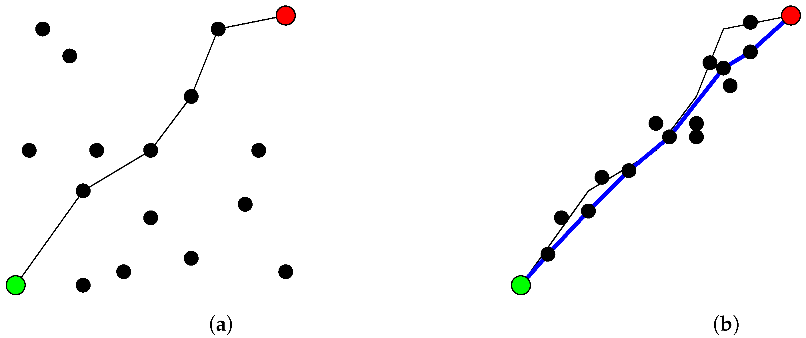
2.2. Trajectory Generation Algorithm
2.3. Graph-Based Path Planning Algorithm
- Two samples are considered neighbors if their distance is below a given radius;
- The graph construction and path search are performed concurrently;
- If the locally-optimal connection to a new sample intersects an obstacle, the algorithm skips this sample. It does not consider the other connections to the neighborhood.
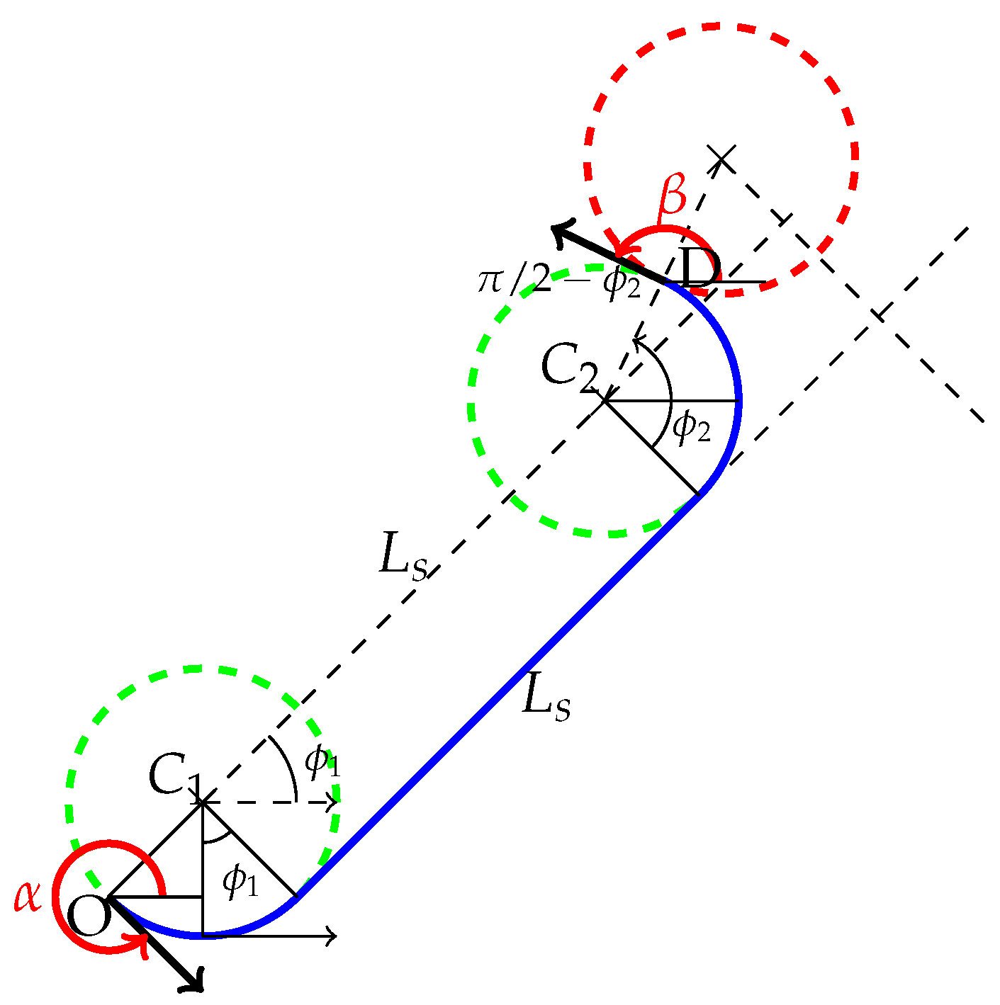
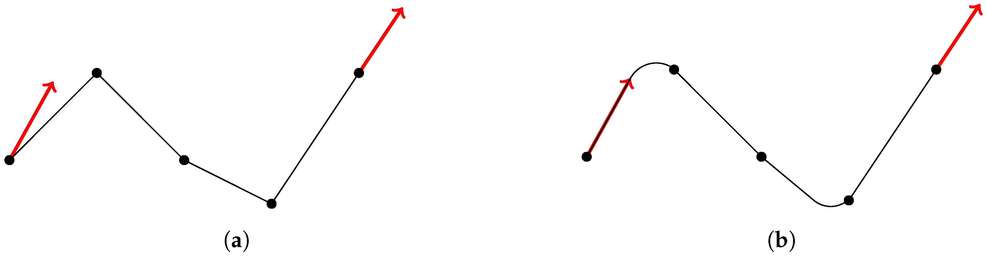
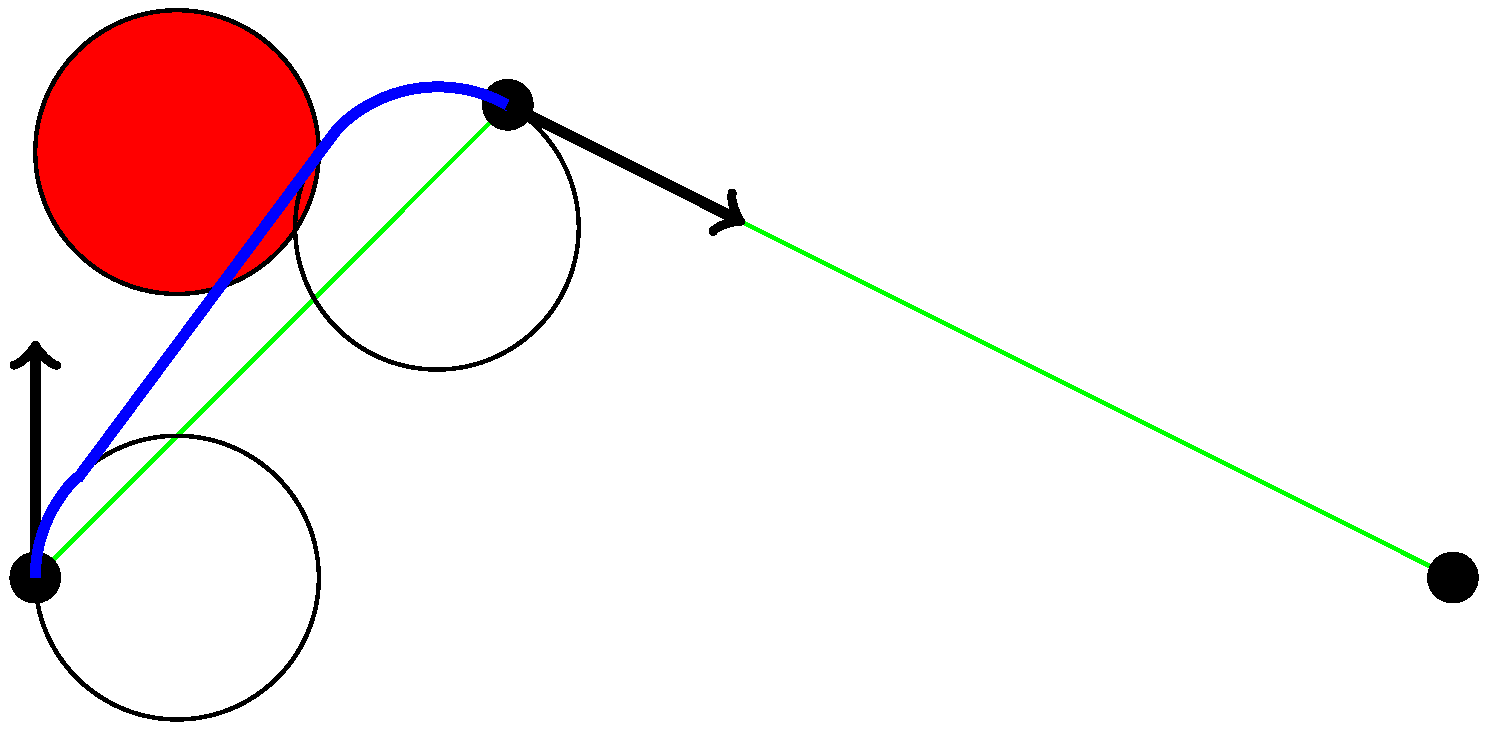
2.4. Dubins Curve
3. Mathematical Modeling
3.1. Search Space
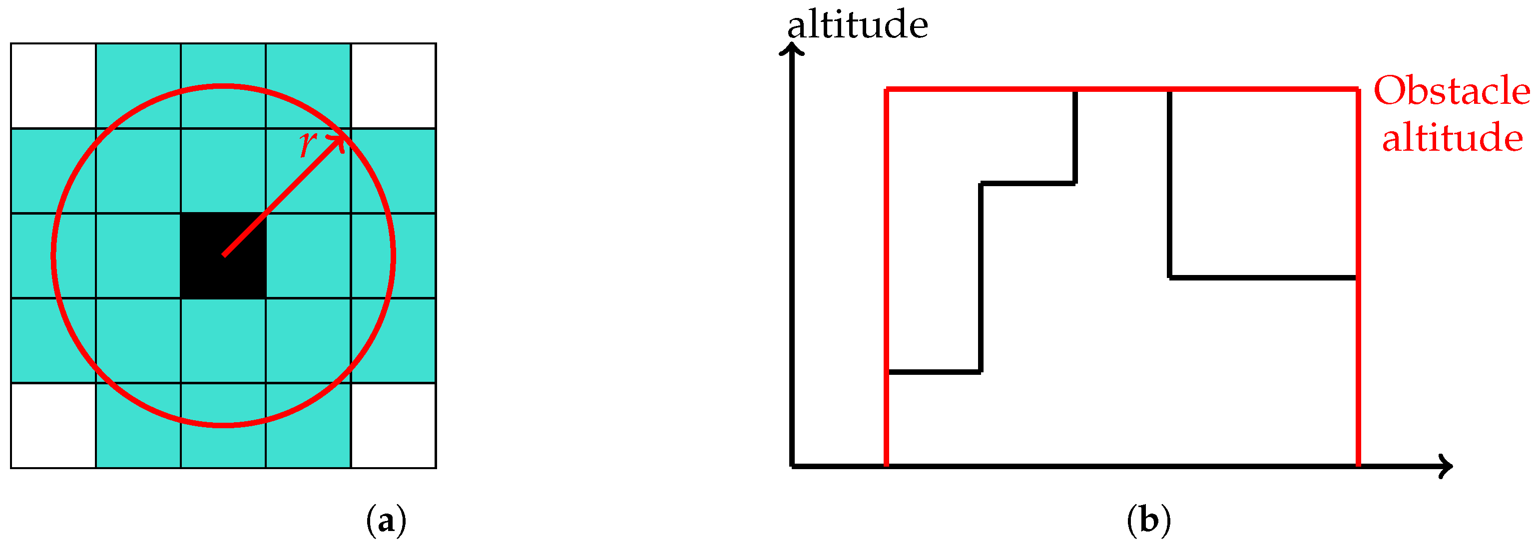
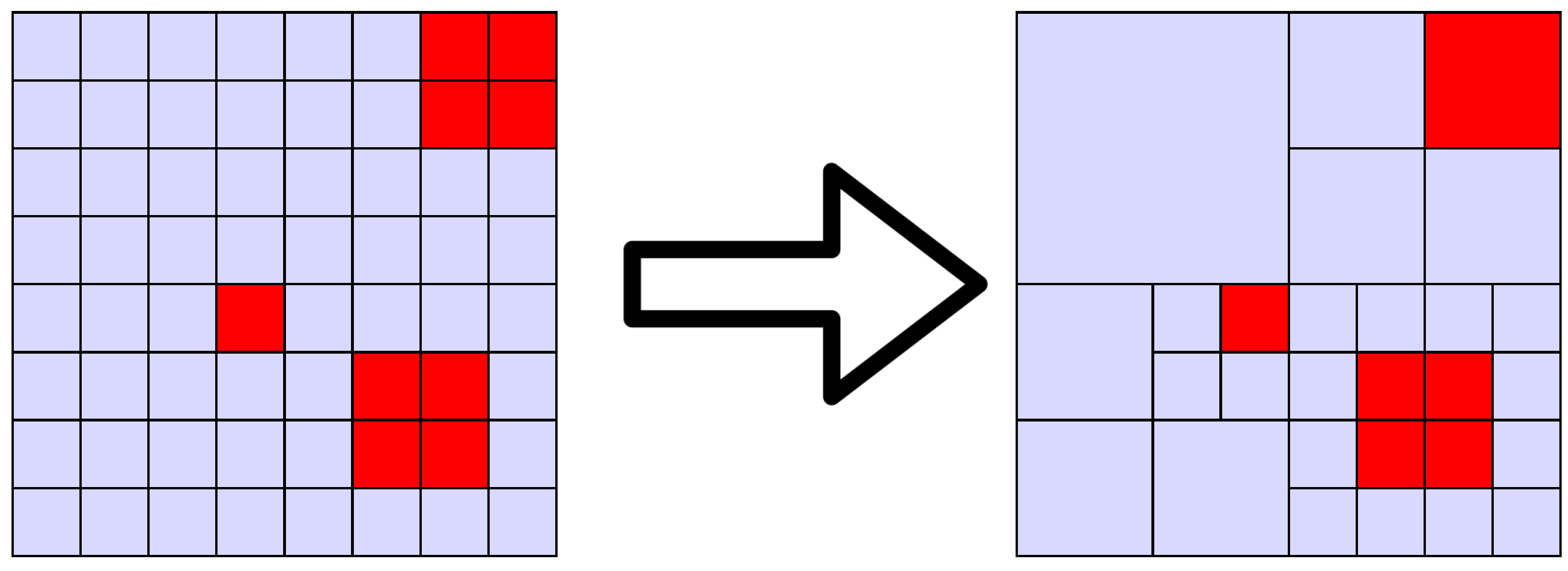
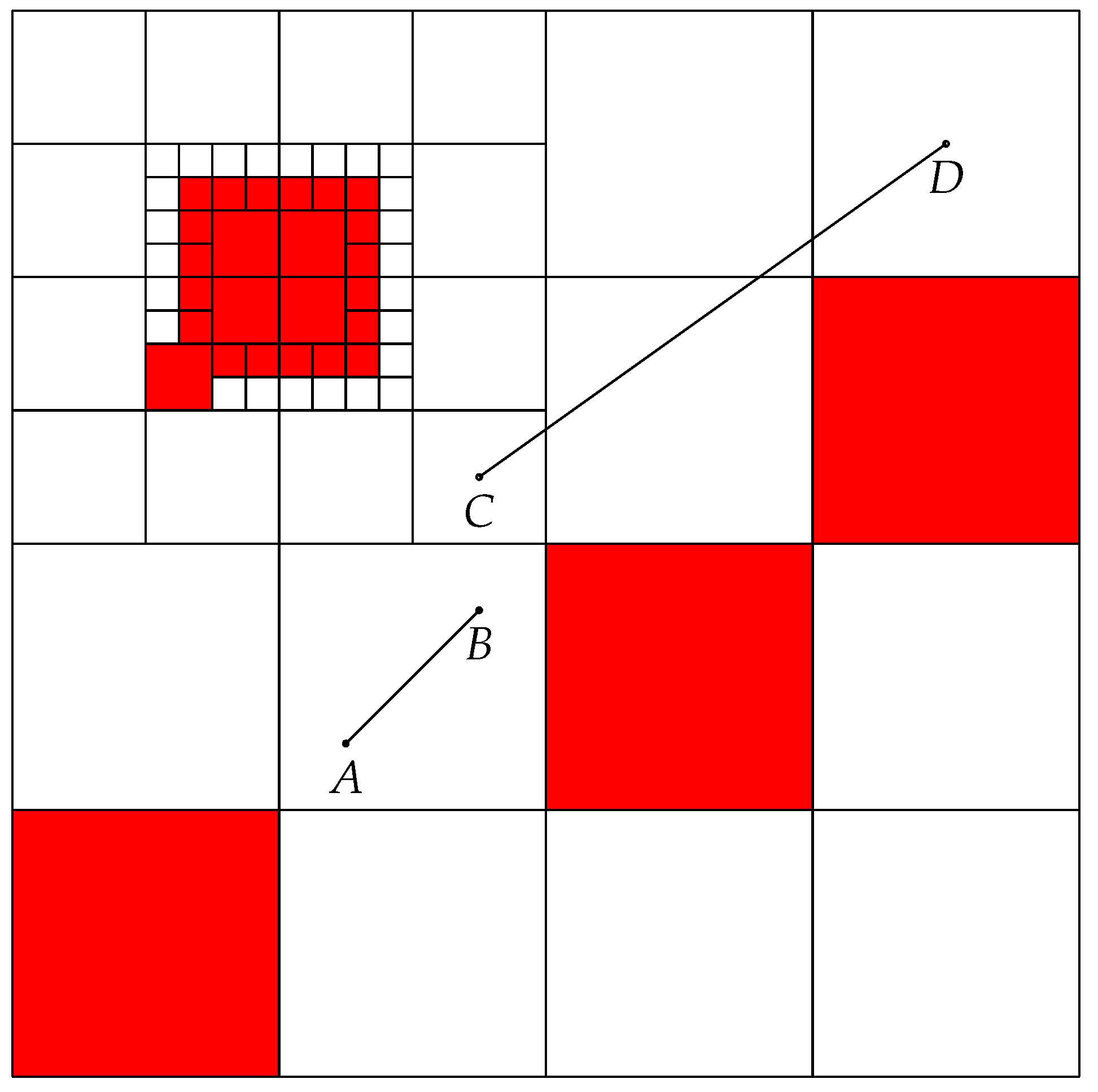
3.1.1. Terrain Data
3.1.2. Route Representation
3.1.3. Objective Function
3.2. Aeronautical Considerations
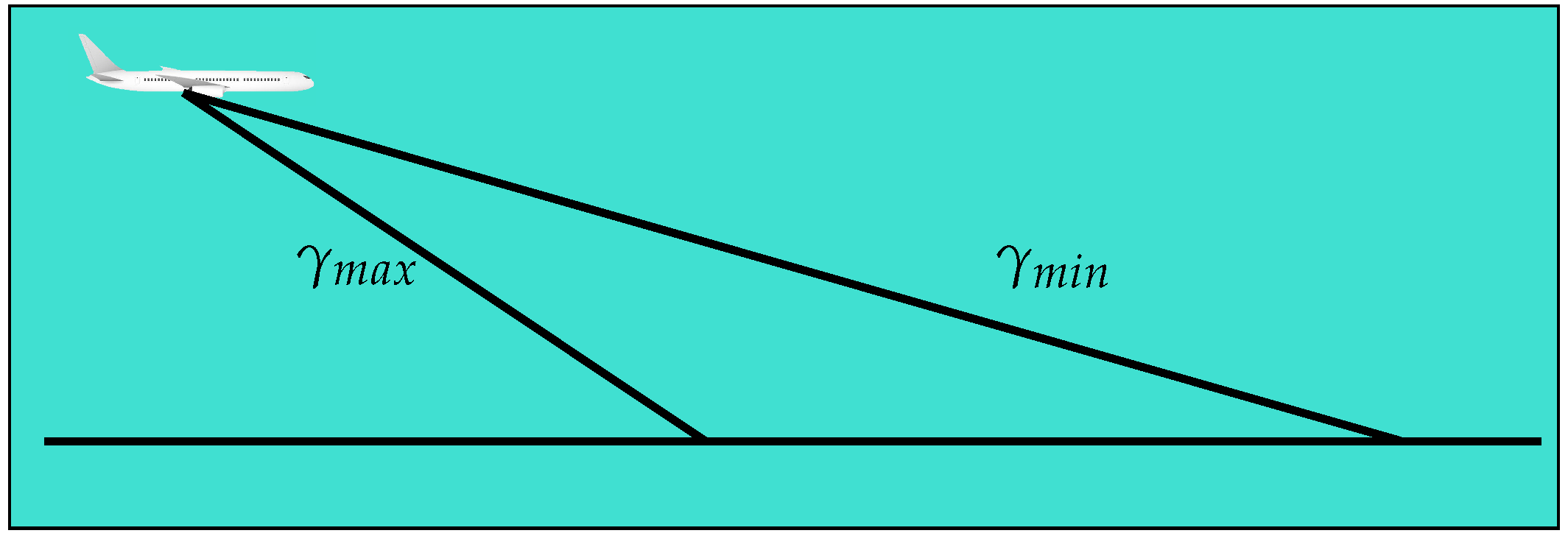
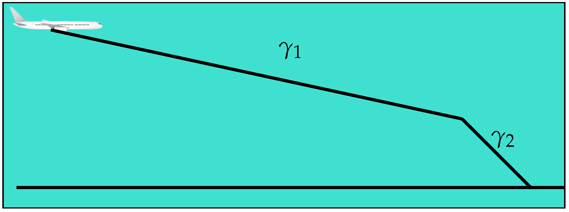
3.2.1. Descent Constraints
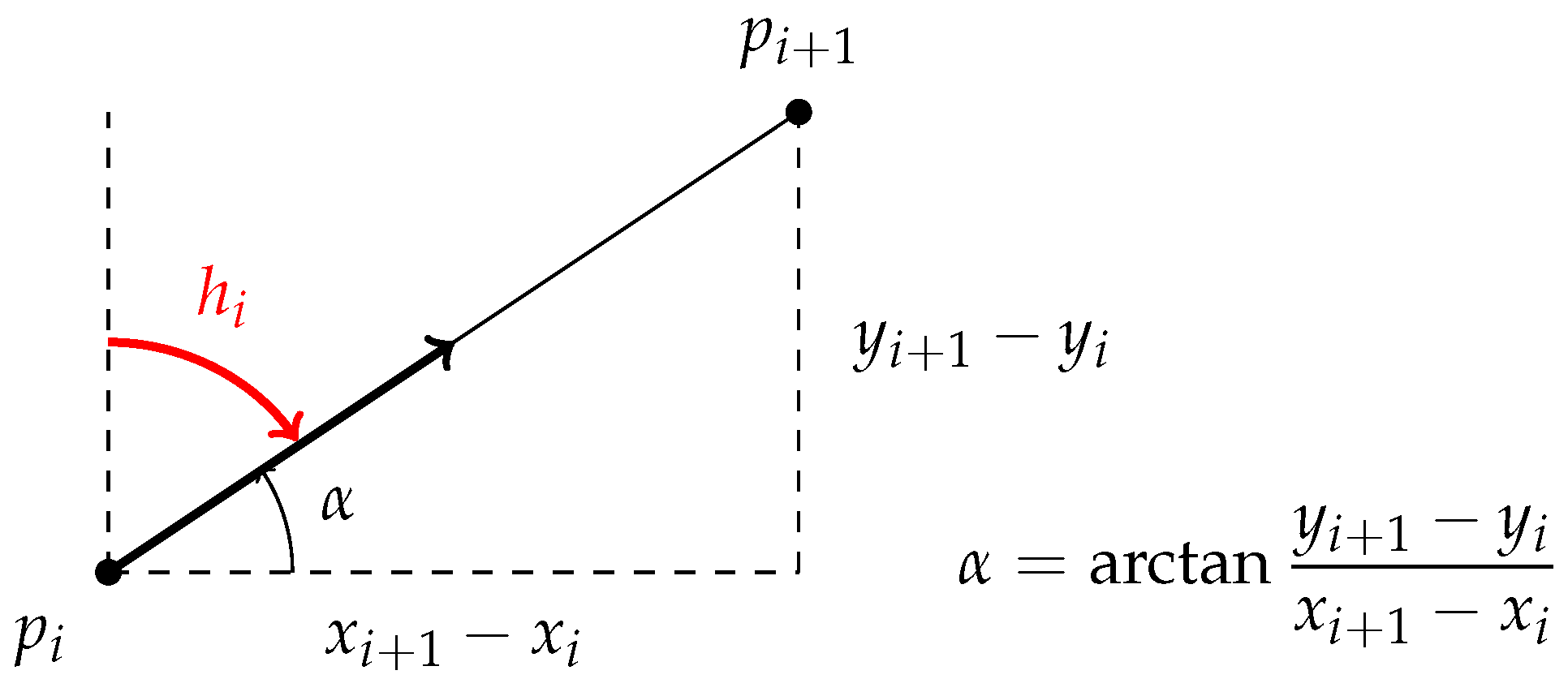
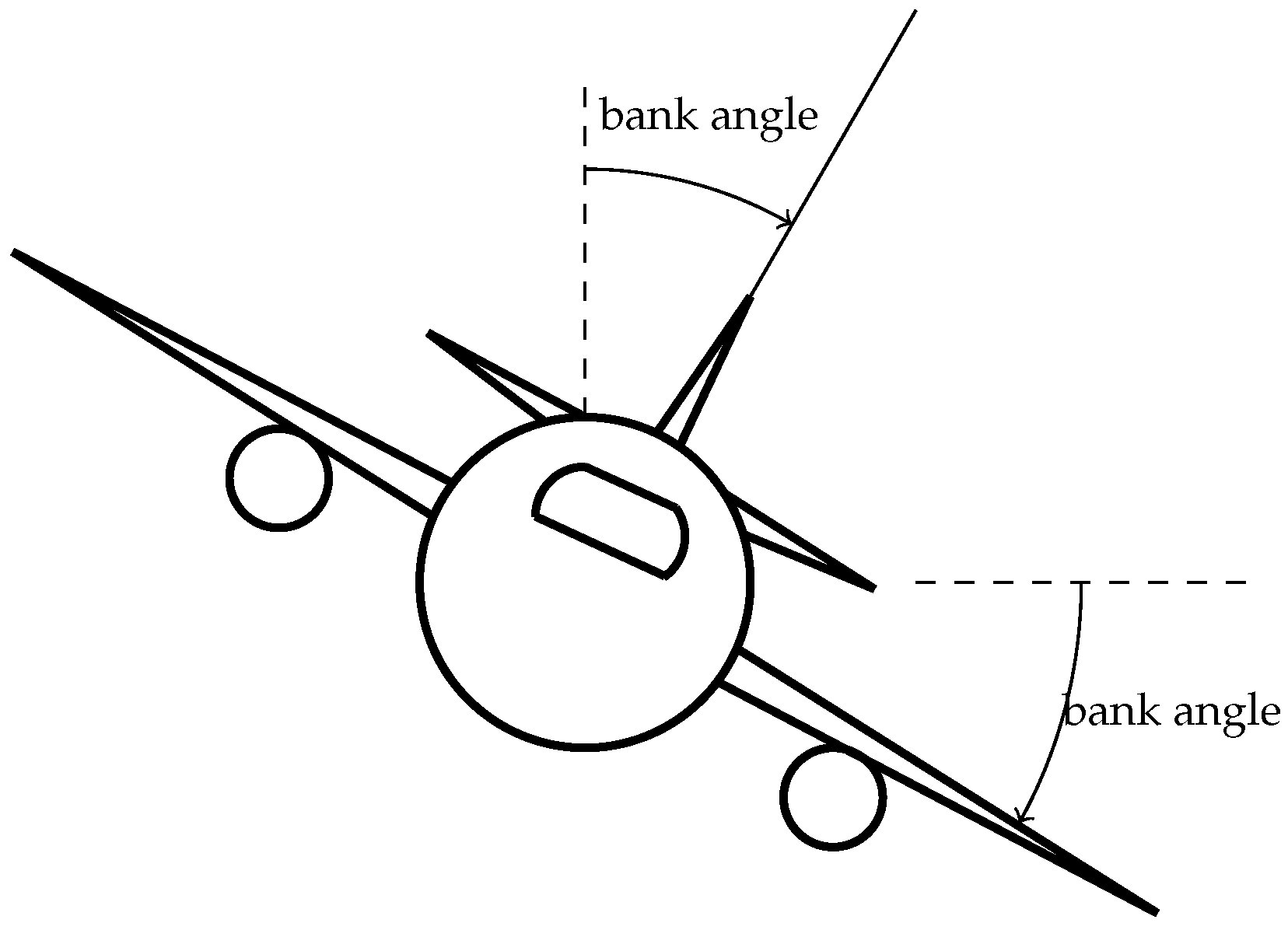
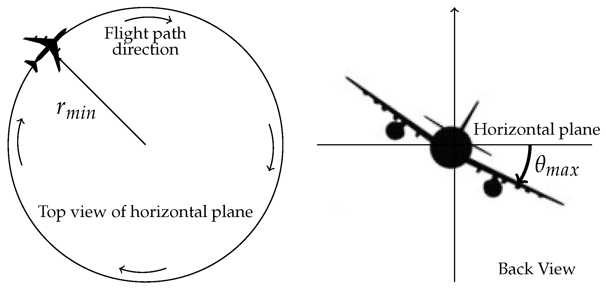
3.2.2. Heading Constraints
- At the time of the declaration of the emergency, the aircraft has a given orientation. The proposed trajectory has to start with this orientation.
- Throughout the flight, the aircraft has to avoid obstacles. For this, it makes turns which are constrained by the maximal bank angle, which depends on aircraft features. This value is associated with the minimal curvature radius. In this study, this radius is considered to be constant. The turns are modeled by means of Dubins curves.
- The final heading of the aircraft has to be the same as the runway or the landing site orientation.
4. Flyable Trajectory Generation
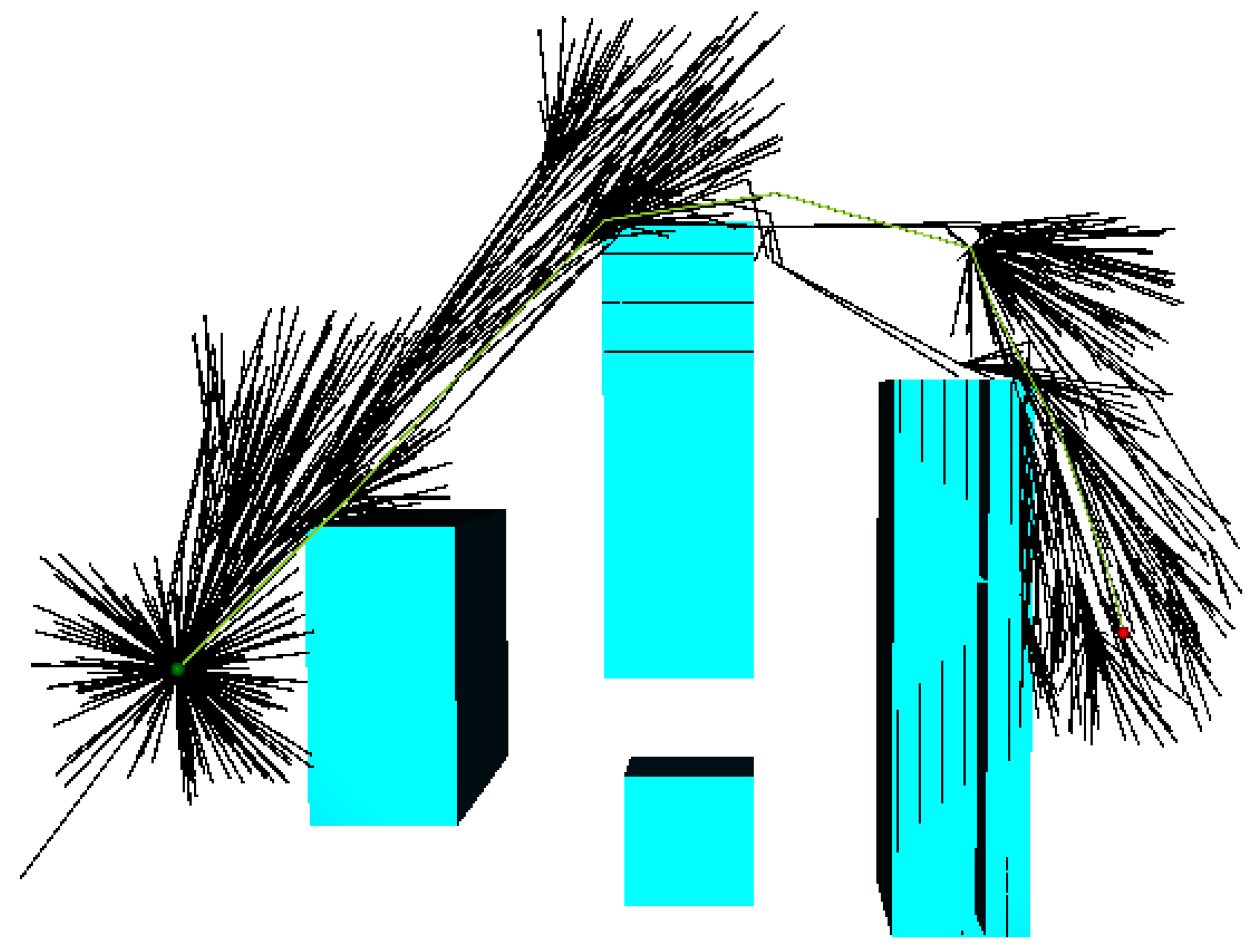
4.1. Algorithm Description
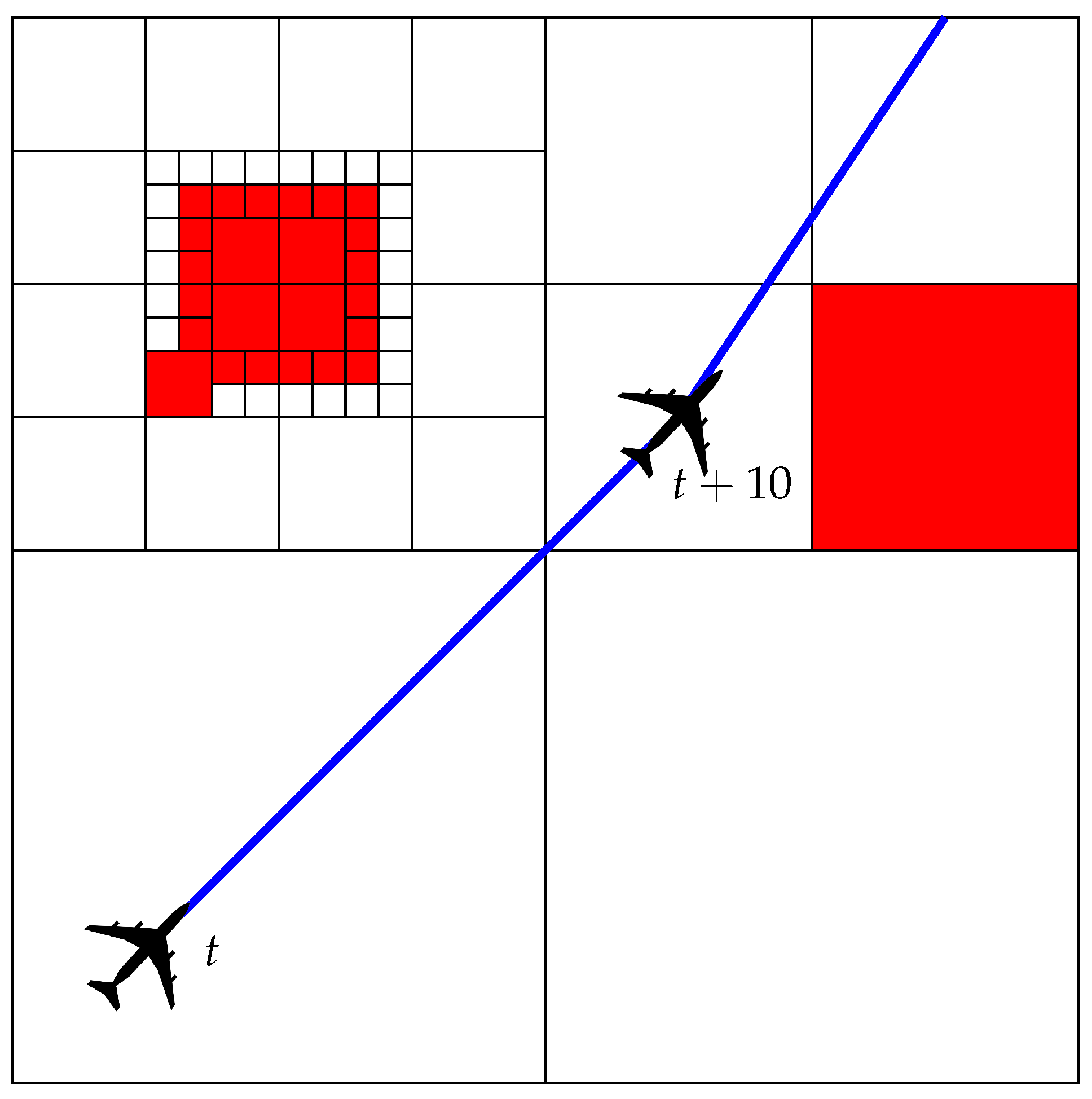
4.2. Improvement of the Free Space Checker
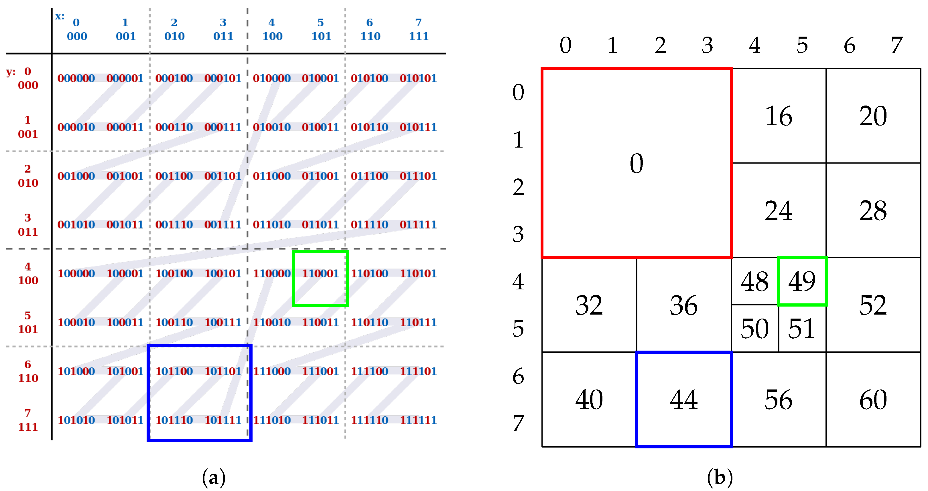
| Algorithm 1 Free space checker: from the start position () and the end position (), the two associated Morton codes are computed and then a dichotomy is performed to check that the segment is in the free space. |
|
5. Results
5.1. Description of the Test Method
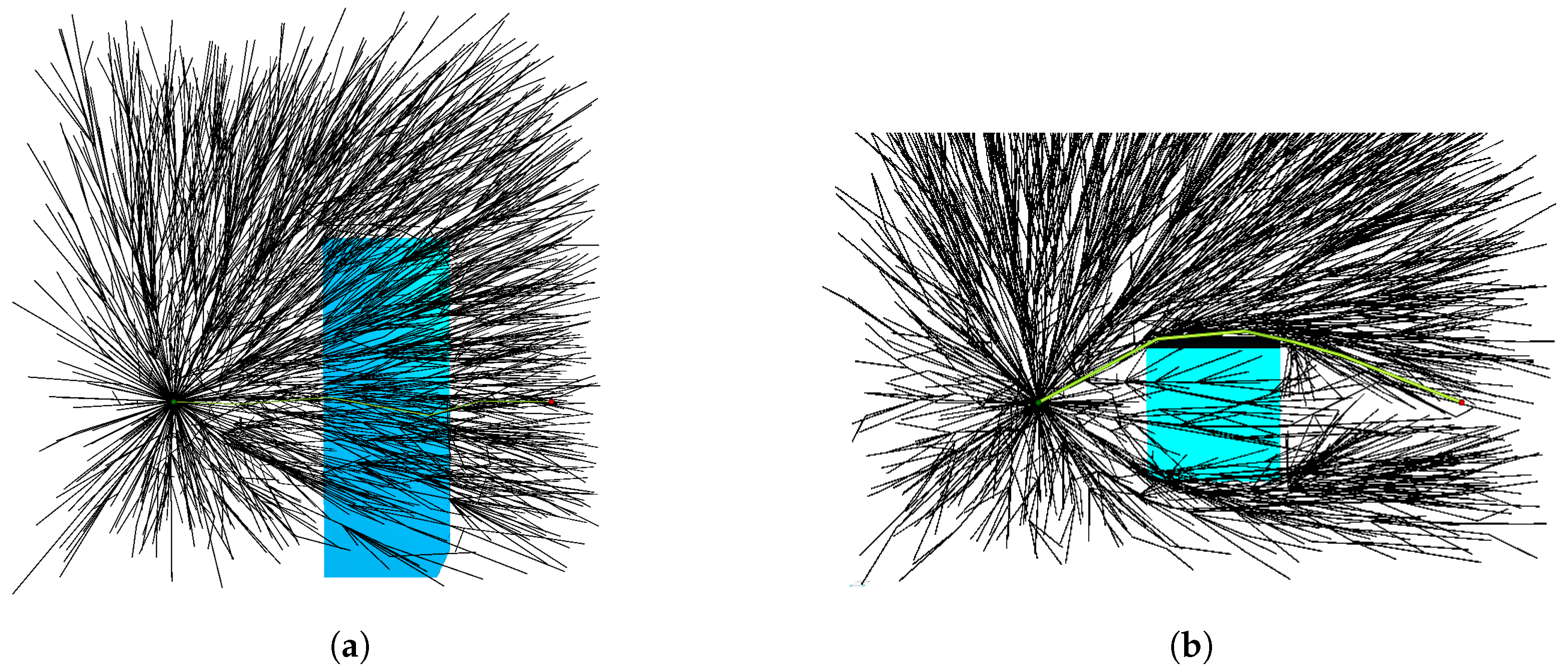
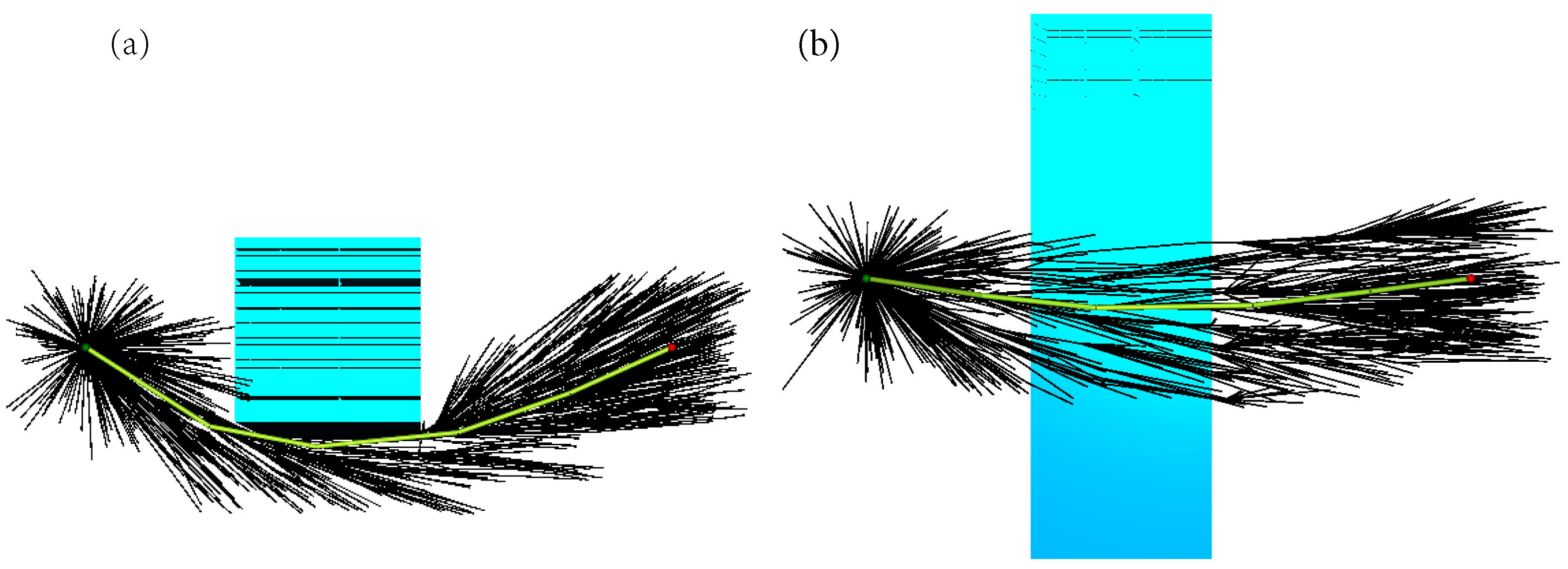
5.2. Simple Case Test
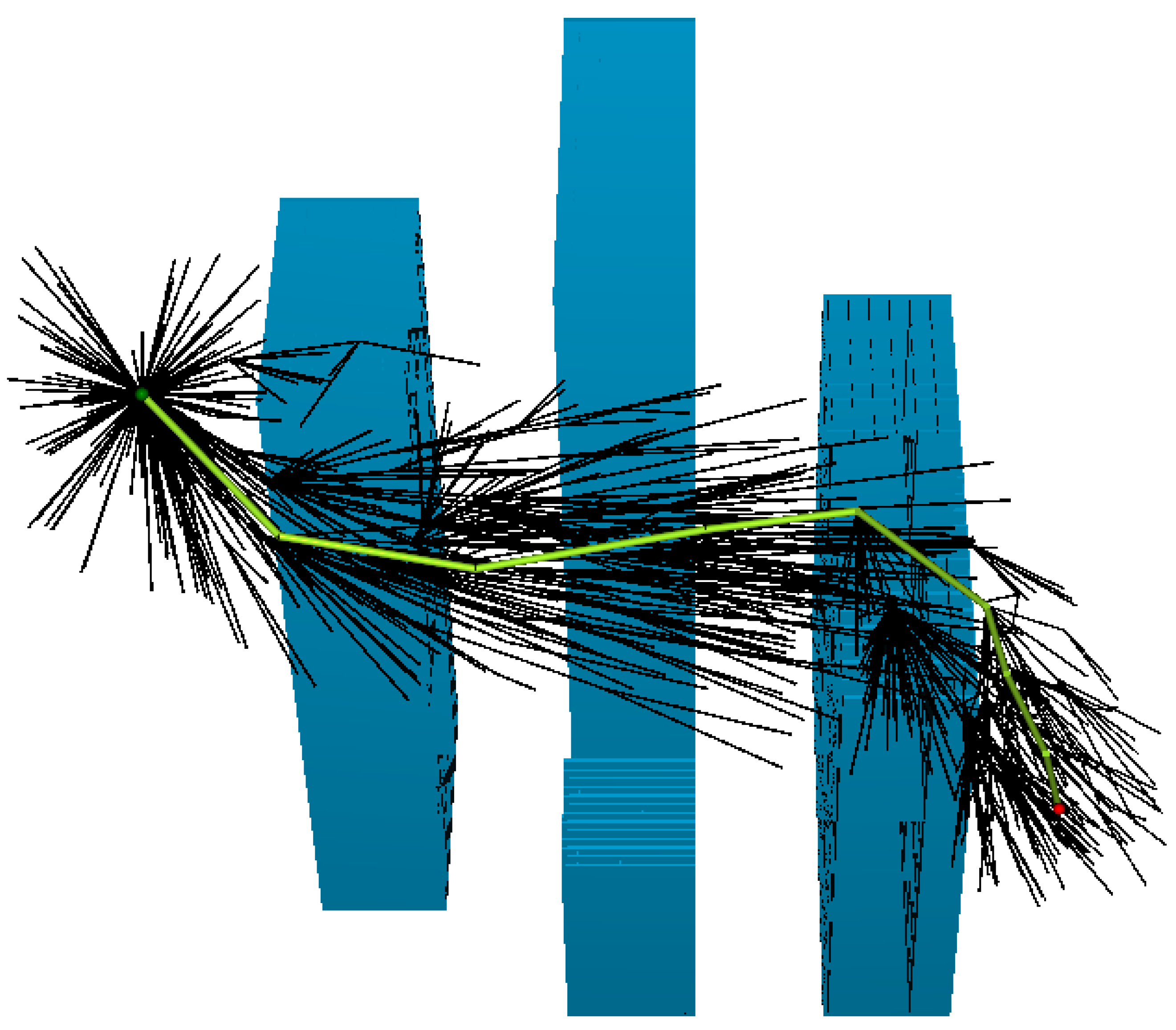
5.3. Multi-Obstacle Case Test
5.4. Computing Time Results
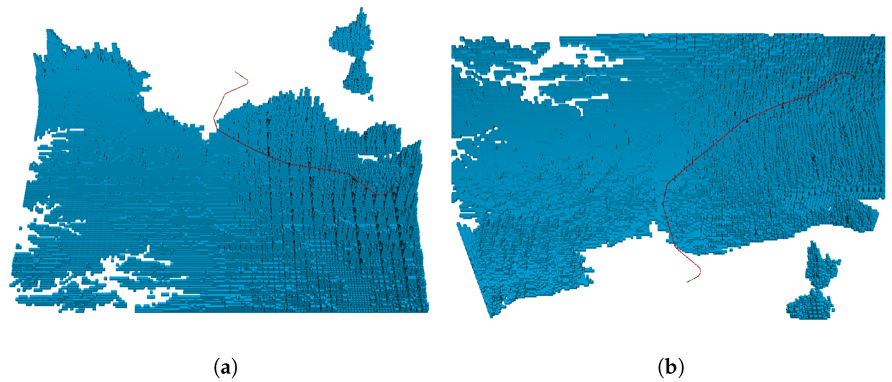
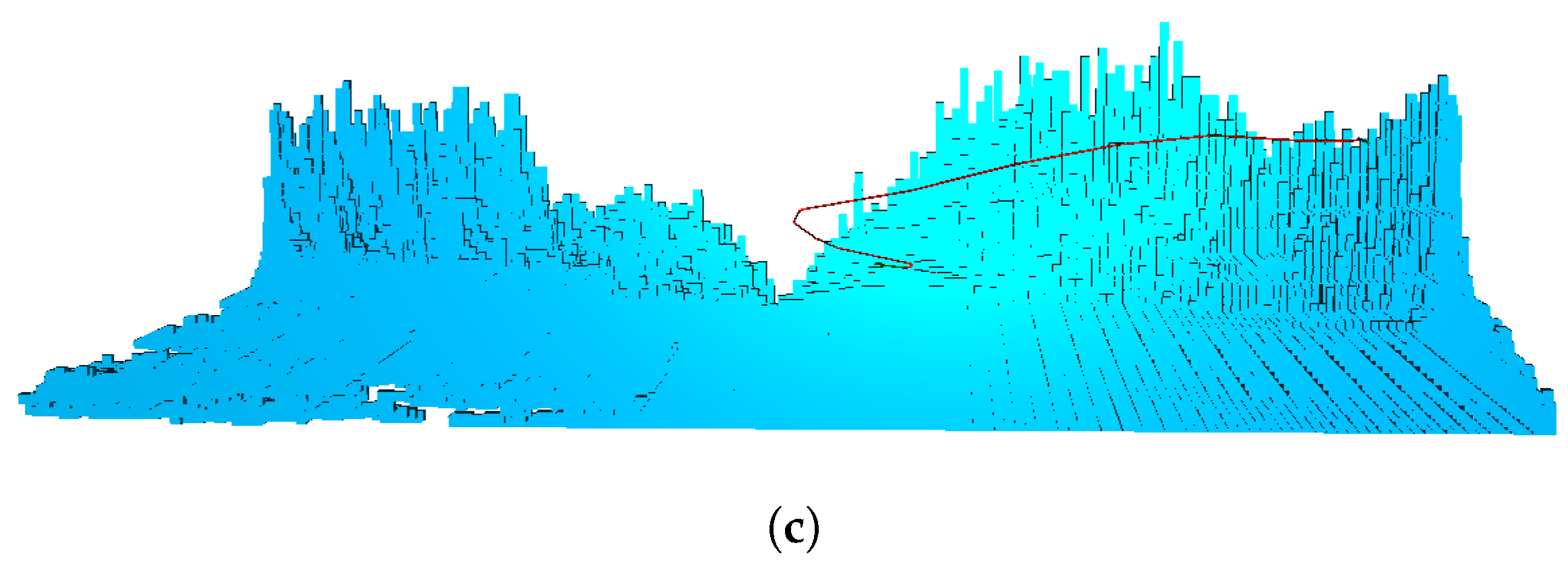
5.5. Real Case Test
6. Conclusions
Author Contributions
Funding
Institutional Review Board Statement
Informed Consent Statement
Data Availability Statement
Acknowledgments
Conflicts of Interest
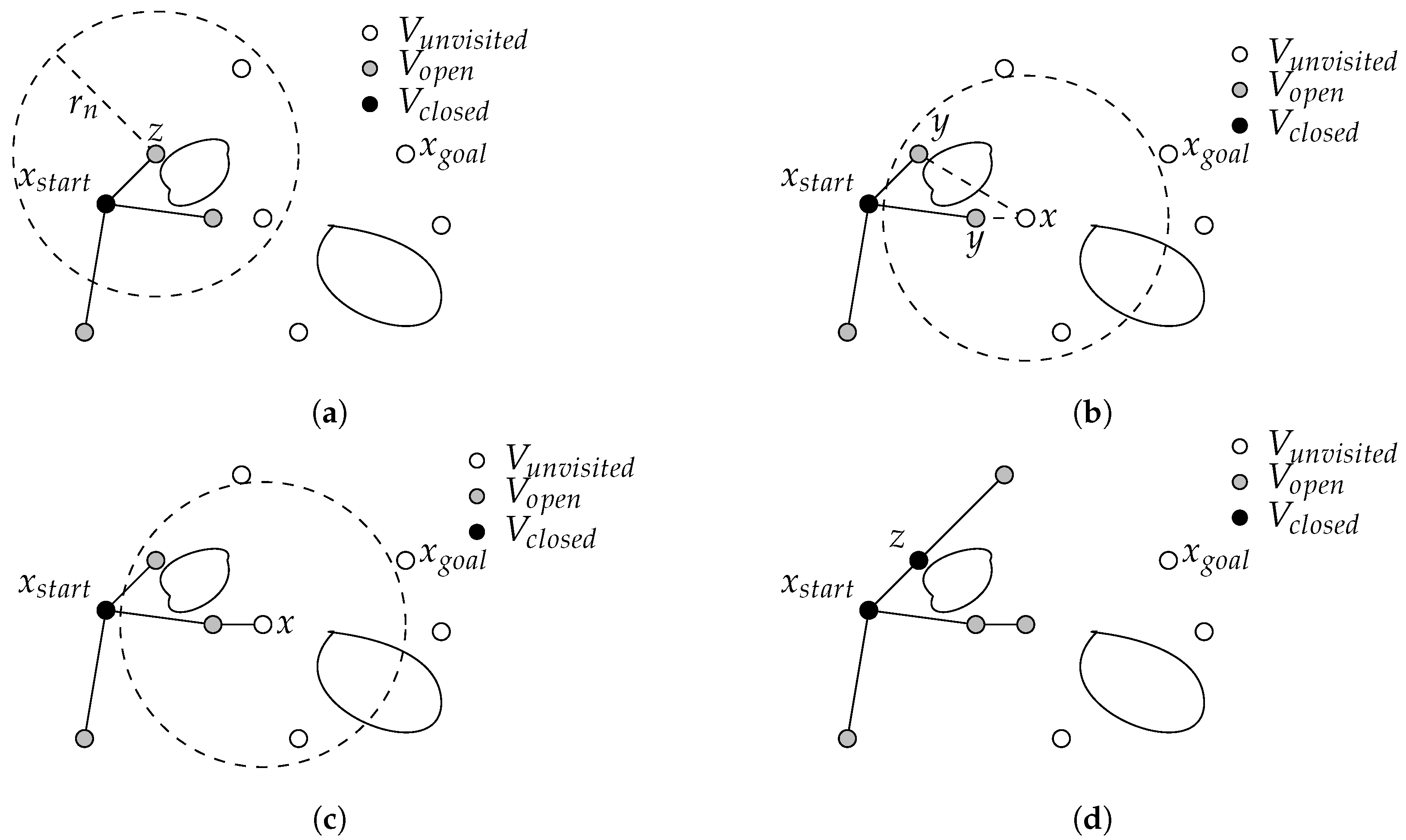
Appendix A. Fast Marching Tree
| Algorithm A1 Fast marching tree: from a sampling composed of n samples, the algorithm creates the graph. At each step, the minimum cost node is selected and the algorithm tries to connect these neighbours (nodes at a distance lower than a radius depending on the number of samples) to the graph [29]. |
|
References
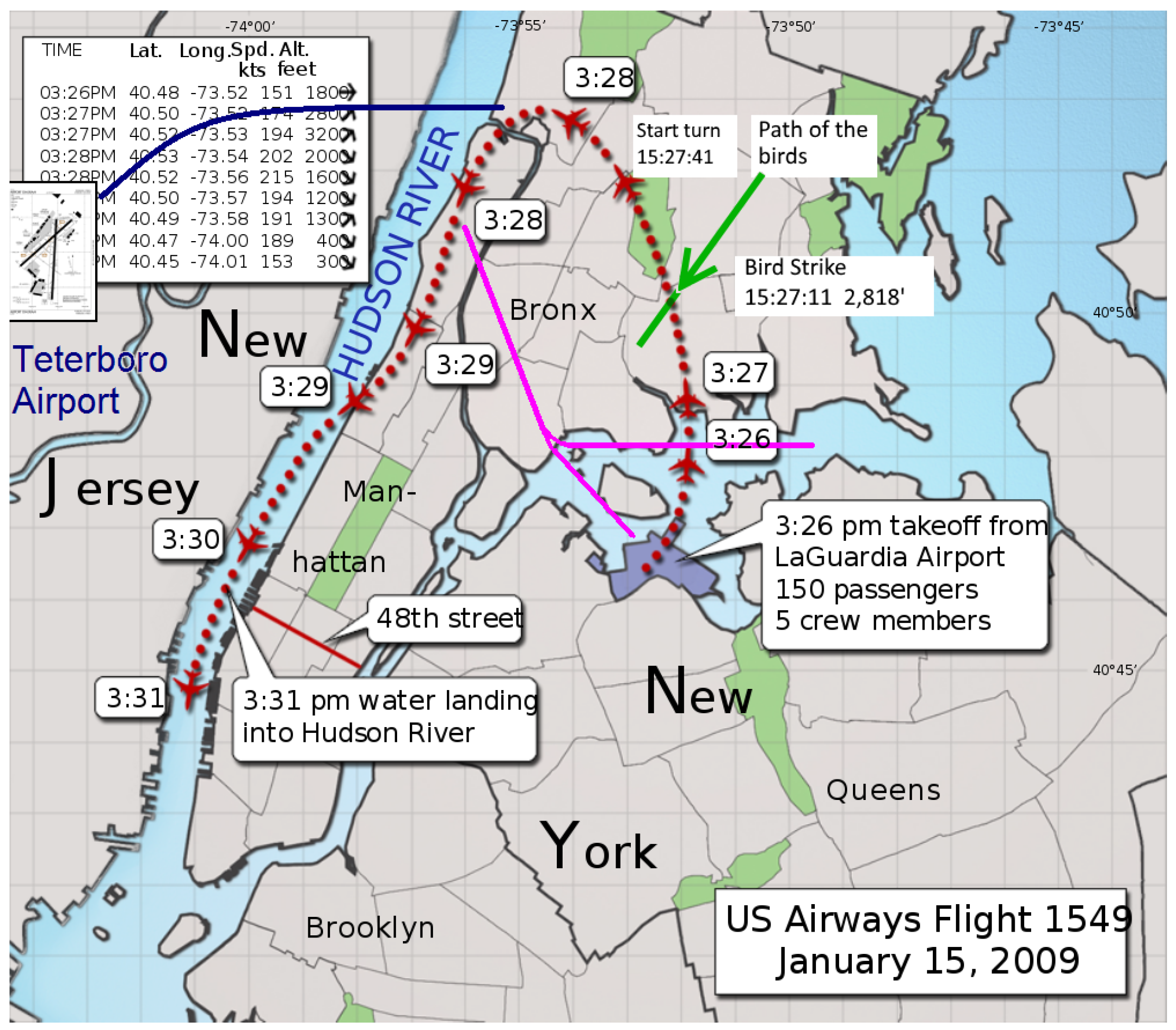
- ChrisnHouston. Trajet du Vol US Airways 1549 le 15 Janvier 2009. 2019. Available online: https://commons.wikimedia.org/wiki/File:Flight_1549-OptionsNotTaken.PNG (accessed on 5 February 2022).
- Atkins, E.M.; Portillo, I.A.; Strube, M.J. Emergency Flight Planning Applied to Total Loss of Thrust. J. Aircr. 2006, 43, 1205–1216. [Google Scholar] [CrossRef] [Green Version]
- Atkins, E.M. Emergency Landing Automation Aids: An Evaluation Inspired by US Airways Flight 1549. AIAA Infotech Aerosp. 2010 2010, 2010, 3381. [Google Scholar]
- Tang, P.; Zhang, S.; Li, J. Final Approach and Landing Trajectory Generation for Civil Airplane in Total Loss of Thrust. Procedia Eng. 2014, 80, 522–528. [Google Scholar] [CrossRef] [Green Version]
- Fallast, A.; Messnarz, B. Automated trajectory generation and airport selection for an emergency landing procedure of CS23 aircraft. DEAS Aeornautical J. 2017, 8, 481–492. [Google Scholar] [CrossRef] [Green Version]
- Zhao, Y. Efficient and Robust Aircraft Landing Trajectory Optimization. Ph.D. Thesis, Georgia Institute of Technology, Atlanta, Georgia, 2012. [Google Scholar]
- Sáez, R.; Khaledian, H.; Prats, X.; Guitart, A.; Delahaye, D.; Feron, E. A Fast and Flexible Emergency Trajectory Generator Enhancing Emergency Geometric Planning with Aircraft Dynamics. In Proceedings of the Fourteenth USA/Europe Air Traffic Management Research and Development Seminar (ATM2021), Virtual, New Orleans, LA, USA, 20–23 September 2021. [Google Scholar]
- Haghighi, H.; Delahaye, D.; Asadi, D. Performance-based emergency landing trajectory planning applying meta-heuristic and Dubins paths. Appl. Soft Comput. 2022, 117, 108453. [Google Scholar] [CrossRef]
- Coxeter, H.S.M. The Problem of Apollonius. Am. Math. Mon. 1968, 75, 5–15. [Google Scholar] [CrossRef]
- Ligny, L.; Guitart, A.; Delahaye, D.; Sridhar, B. Aircraft Emergency Trajectory Design: A Fast Marching Method on a Triangular Mesh. In Proceedings of the Fourteenth USA/Europe Air Traffic Management Research and Development Seminar, Virtual, New Orleans, LA, USA, 20–23 September 2021. [Google Scholar]
- Hong, H.; Piprek, P.; Gerdts, M.; Holzapfel, F. Computationally Efficient Trajectory Generation for Smooth Aircraft Flight Level Changes. J. Guid. Control. Dyn. 2021, 44, 1532–1540. [Google Scholar] [CrossRef]
- Woo, J.W.; An, J.Y.; Cho, M.G.; Kim, C.J. Integration of path planning, trajectory generation and trajectory tracking control for aircraft mission autonomy. Aerosp. Sci. Technol. 2021, 118, 107014. [Google Scholar] [CrossRef]
- Qureshi, A.; Ayaz, Y. Potential Functions based Sampling Heuristic For Optimal Path Planning. Auton. Robot. 2016, 40, 1079–1093. [Google Scholar] [CrossRef] [Green Version]
- Girardet, B.; Lapasset, L.; Delahaye, D.; Rabut, C. Wind-optimal path planning: Application to aircraft trajectories. In Proceedings of the 2014 13th International Conference on Control Automation Robotics & Vision (ICARCV), Singapore, 10–12 December 2014; pp. 1403–1408. [Google Scholar] [CrossRef] [Green Version]
- González, V.; Monje, C.A.; Moreno, L.; Balaguer, C. Fast Marching Square Method for UAVs Mission Planning with consideration of Dubins Model Constraints. IFAC-PapersOnLine 2016, 49, 164–169. [Google Scholar] [CrossRef]
- Yu, Y.H.; Zhang, Y.T. Collision avoidance and path planning for industrial manipulator using slice-based heuristic fast marching tree. Robot.-Comput.-Integr. Manuf. 2022, 75, 102289. [Google Scholar] [CrossRef]
- Tehrani, N.D.; Cherepinsky, I.; Carlson, S. Closed-loop Fast Marching Tree (CL-FMT*) with Application to Helicopter Landing Trajectory Planning. In Proceedings of the 2021 IEEE/RSJ International Conference on Intelligent Robots and Systems (IROS), Prague, Czech Republic, 27 September–1 October 2021; pp. 346–351. [Google Scholar] [CrossRef]
- Kang, J.G.; Choi, Y.S.; Jung, J.W. A Method of Enhancing Rapidly-Exploring Random Tree Robot Path Planning Using Midpoint Interpolation. Appl. Sci. 2021, 11, 8483. [Google Scholar] [CrossRef]
- Dijkstra, E.W. A note on two problems in connexion with graphs. Numer. Math. 1959, 1, 269–271. [Google Scholar] [CrossRef] [Green Version]
- Ford, L.R., Jr. Network Flow Theory; RAND Corporation: Santa Monica, CA, USA, 1956. [Google Scholar]
- Bellman, R. On a routing problem. Q. Appl. Math. 1958, 16, 87–90. [Google Scholar] [CrossRef] [Green Version]
- Hart, P.; Nilsson, N.; Raphael, B. A Formal Basis for the Heuristic Determination of Minimum Cost Paths. IEEE Trans. Syst. Sci. Cybern. 1968, 4, 100–107. [Google Scholar] [CrossRef]
- Gammell, J.D.; Srinivasa, S.S.; Barfoot, T.D. Informed RRT*: Optimal Sampling-based Path Planning Focused via Direct Sampling of an admissible Ellipsoidal Heuristic. In Proceedings of the IEEE/RSJ International Conference on Intelligent Robots and Systems, Chicago, IL, USA, 14–18 September 2014. [Google Scholar]
- Gammell, J.; Srinivasa, S.; Barfoot, T. Bit*: Batch informed trees for optimal sampling-based planning via dynamic programming on implicit random geometric graphs. In Proceedings of the 2015 IEEE International Conference on Robotics and Automation, Seattle, WA, USA, 26–30 May 2015. [Google Scholar]
- Pharpatara, P.; Hérissé, B.; Bestaoui, Y. 3-D Trajectory Planning of Aerial Vehicles Using RRT*. IEEE Trans. Control. Syst. Technol. 2017, 25, 1116–1123. [Google Scholar] [CrossRef] [Green Version]
- Karaman, S.; Frazzoli, E. Incremental sampling-based algorithms. In Robotics Science and Systems VI; MIT Press: Cambridge, MA, USA, 2010. [Google Scholar]
- Gammell, J.D.; Strub, M.P. Asymptotically Optimal Sampling-Based Motion Planning Methods. Annu. Rev. Control. Robot. Auton. Syst. 2021, 4, 295–318. [Google Scholar] [CrossRef]
- Karaman, S.; Frazzoli, E. Sampling-based Algorithms for Optimal Motion Planning. Int. J. Robot. Res. 2011, 30, 846–894. [Google Scholar] [CrossRef]
- Janson, L.; Schmerling, E.; Clark, A.; Pavone, M. Fast Marching Tree: A Fast Marching Sampling-Based Method for Optimal Motion Planning in Many Dimension. Int. J. Robot. Res. 2015, 34, 883–921. [Google Scholar] [CrossRef]
- Huifang, W.; Lucia, P.; Antonio, B. Motion planning for Formations of Dubins Vehicles. In Proceedings of the 49th IEEE Conference on Decision and Control, Atlanta, GA, USA, 15–17 December 2010. [Google Scholar]
- Gianfranco, P. Shortest paths for Dubins vehicles in presence of via points. IFAC-PapersOnLine 2019, 52, 295–300. [Google Scholar]
- Satyanarayana, G.; Manyam, D.C.; Von Moll, A.L.; Fuchs, Z. Shortest Dubins Path to a circle. In Proceedings of the AIAA Scitech 2019 Forum, San Diego, CA, USA, 7–11 January 2019. [Google Scholar]
- Le Ny, J.; Feron, E.; Frazzoli, E. On the Dubins Traveling Salesman Problem. IEEE Trans. Autom. Control. 2012, 57, 265–270. [Google Scholar] [CrossRef]
- Baklouti, Z. Système de Planification de Chemins Aériens en 3D: Préparation de Missions et Replanification en cas d’Urgence. Ph.D. Thesis, Université Polytechnique Hauts de France, Valenciennes, France, 2018. [Google Scholar]
- Kunio, A.; Koyo, M.; Shintaro, K.; Ryosuke, K.; Jia, F. Constant time neighbor finding in quadtrees: An experimental result. In Proceedings of the 2008 3rd International Symposium on Communications, Control and Signal Processing, Saint Julian’s, Malta, 12–14 March 2008. [Google Scholar]
- Morton, G.M. A Computer Oriented Geodetic Data Base; and a New Technique in File Sequencing; Technical Report; IBM: Ottawa, ON, Canada, 1966. [Google Scholar]
- Gargantini, I. An effective way to represent quadtrees. Commun. ACM 1982, 25, 905–910. [Google Scholar] [CrossRef]
- Chang, H.K.C.; Liu, J.L. A linear quadtree compression scheme for image encryption. Signal Process. Image Commun. 1997, 10, 279–290. [Google Scholar] [CrossRef]
- Eppstein, D. Z-Order Curve. 2010. Available online: https://commons.wikimedia.org/wiki/File:Z-curve.svg (accessed on 5 February 2022).


| Graph Generation | Time Complexity | Space | |
|---|---|---|---|
| Algorithm | Processing | Query | Complexity |
| PRM | |||
| PRM* | |||
| RRT | |||
| RRT* | |||
| FMT | |||
| Error (%) | FMT | Proposed FMT |
|---|---|---|
| 5 | 98.7 | 51.3 |
| 2 | 493.8 | 203.4 |
| 1 | 6896.5 | 2057.3 |
Publisher’s Note: MDPI stays neutral with regard to jurisdictional claims in published maps and institutional affiliations. |
© 2022 by the authors. Licensee MDPI, Basel, Switzerland. This article is an open access article distributed under the terms and conditions of the Creative Commons Attribution (CC BY) license (https://creativecommons.org/licenses/by/4.0/).
Share and Cite
Guitart, A.; Delahaye, D.; Feron, E. An Accelerated Dual Fast Marching Tree Applied to Emergency Geometric Trajectory Generation. Aerospace 2022, 9, 180. https://doi.org/10.3390/aerospace9040180
Guitart A, Delahaye D, Feron E. An Accelerated Dual Fast Marching Tree Applied to Emergency Geometric Trajectory Generation. Aerospace. 2022; 9(4):180. https://doi.org/10.3390/aerospace9040180
Chicago/Turabian StyleGuitart, Andréas, Daniel Delahaye, and Eric Feron. 2022. "An Accelerated Dual Fast Marching Tree Applied to Emergency Geometric Trajectory Generation" Aerospace 9, no. 4: 180. https://doi.org/10.3390/aerospace9040180
APA StyleGuitart, A., Delahaye, D., & Feron, E. (2022). An Accelerated Dual Fast Marching Tree Applied to Emergency Geometric Trajectory Generation. Aerospace, 9(4), 180. https://doi.org/10.3390/aerospace9040180