1. Introduction
A tiltrotor aircraft is a hybrid aircraft that combines the hover capability of a helicopter with the speed and range of an airplane [
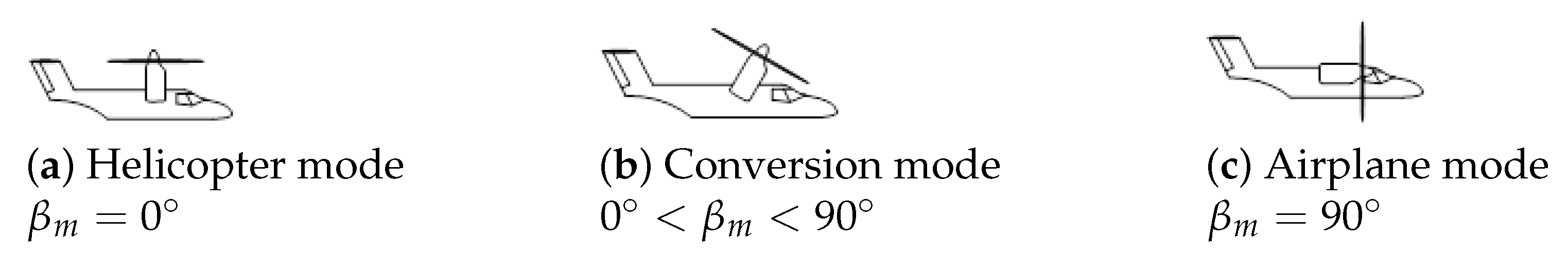
1], i.e., it has the features of both a helicopter and a fixed-wing aircraft. With the nacelles vertical, it uses the rotor-generated thrust to take off like a helicopter, and with the nacelles horizontal, it uses the thrust to move forward like a fixed-wing aircraft. The most well-known tiltrotor aircraft is the XV-15. The XV-15 tiltrotor was jointly developed by the U.S. Army, NASA and the U.S. Navy. As shown in
Figure 1, the tiltrotor has three flight modes: helicopter mode, when nacelle angle is 0°, airplane mode, when nacelle angle is 90°, and conversion mode, when nacelle angle is between 0° and 90°.
The airspeed limits for each nacelle angle between helicopter mode and airplane mode are dictated by the conversion corridor, which ensures the aircraft will operate safely at a nacelle angle over a certain speed range. The flight mode between helicopter mode and airplane mode is called conversion flight mode. The conversion corridor is the most unique part of the tiltrotor aircraft.
In the recent years, advances in the field of automatic controls for tiltrotor aircrafts have been made [
2,
3,
4,
5]. Generally, the model is linearized on different nacelle angles at which the separate control schemes are designed, and then the control law is switched based on the nacelle angles. Whilst the scheme is attractive, it may not guarantee the stability of the system, other than at the points of design, or the required performance. A neural-network augmented model inversion control is used to provide a civilian tiltrotor aircraft with consistent response characteristics throughout its operating envelope. The proposed method can alleviate the requirement of the extensive gain scheduling with tiltrotor nacelle angle and speed [
6]. An improved gain-scheduled flight controller was designed for a quad-tilt-wing unmanned aerial vehicle, which consists of a gain-scheduled stability control augmentation system (SCAS), a gain-scheduled control augmentation system and a gain-scheduled turn coordinator [
7]. Seongwook Choi proposed a rate stability augmentation system and an attitude stability and control augmentation system for a small tiltrotor unmanned aerial vehicle. Flight tests verified that the control algorithm worked well [
8]. A model inversion-based flight control system was developed for an XV-15 tiltrotor aircraft simulation model by Thanan Yomchinda [
9], and the system was evaluated for handling qualities across a predefined envelope. The results showed that model inversion control can provide an effective design tool for the flight control of the tiltrotor aircraft. An improved back propagation (BP) neural network PID control algorithm was proposed for the tiltrotor flight control system in conversion mode [
10]. By combining the model inversion control with an adaptive neural network, a flight control design was presented in [
11]. In [
12], the passive and active controls on aerodynamic interactions of a tiltrotor aircraft were investigated in hovering flight. In the transition process of incline take-off, an innovative trim method was introduced to a tiltrotor aircraft’s flight control in [
13]. In [
14], a flight control system for a tiltrotor UAV was synthesized based on an incremental nonlinear dynamic inversion technique. Effector redundancy was managed to develop a control allocation module for distributing control effort among the available actuators, based on their availability and effectiveness.
The conversion of flight control is the most challenging problem of tiltrotor aircrafts because during the conversion process, such aircrafts are characterized by highly nonlinear and strongly coupled dynamics and large modeling uncertainties, which results in a very difficult control problem compared to that of conventional airplanes. In the current literature, there are not many reasonable or better methods to solve the conversion flight control problem of tiltrotor aircrafts. This paper proposes an technique combining ADRC with SMC for tiltrotor aircrafts. The approach applied in this paper is motivated by the need to ensure the validity of the practical model. ADRC, an effective control method originally proposed by Han in [
15,
16] and developed in-depth by Gao in [
17], has been utilized in different fields in recent years. It does not depend on the accurate mathematical model of planes. The key technique in ADRC is the use of an extended state observer (ESO), which estimates and compensates the internal (such as model uncertainty) and external disturbances of a system online. With a nonlinear control strategy, ADRC can achieve better static and dynamic performances, strong robustness and adaptability. More achievements of ADRC can be found in [
18,
19,
20,
21,
22]. As a powerful nonlinear control method, sliding mode control is widely used in various applications, such as that of [
23,
24]. However, to some extent, integrated SMC and ADRC is still rare, especially in the control of the tiltrotor aircraft. This motivates us to investigate a sliding-mode-based active disturbance rejection control for the tiltrotor aircraft. The main contributions of this paper are given as follows. Based on the designed conversion path, a separate control allocator is devoted to the control effort distribution among available effectors. Finally, the flight control system is analyzed and synthesized by using the inner/outer loop control structure, and the ADRCs including ESOs and control laws are developed for coupling flight systems, in consideration of model uncertainties estimated by ESOs to realize accuracy control of the tiltrotor aircraft.
This paper is outlined as follows: In
Section 2, the simplification of the three-channel coupling nonlinear model with six degrees of freedom is studied. In
Section 3, the control laws are given for the conversion flight mode, including the control allocation strategy, outer-loop control law design, inner-loop thrust control law and attitude control law design. In
Section 4, the simulation results and evaluation of the performance of the scheme proposed are given, followed by a conclusion in
Section 5.
2. Model Simplifying of Longitudinal Channel
To effectively control a tiltrotor aircraft, a mathematical model should first be established to describe the dynamics of a tiltrotor aircraft. Results of this paper are based on the configuration and parameters of the XV-15 tiltrotor aircraft. The basic parameters of the XV-15 tiltrotor aircraft are shown in
Table 1, and the whole parameters can be found in [
25,
26].
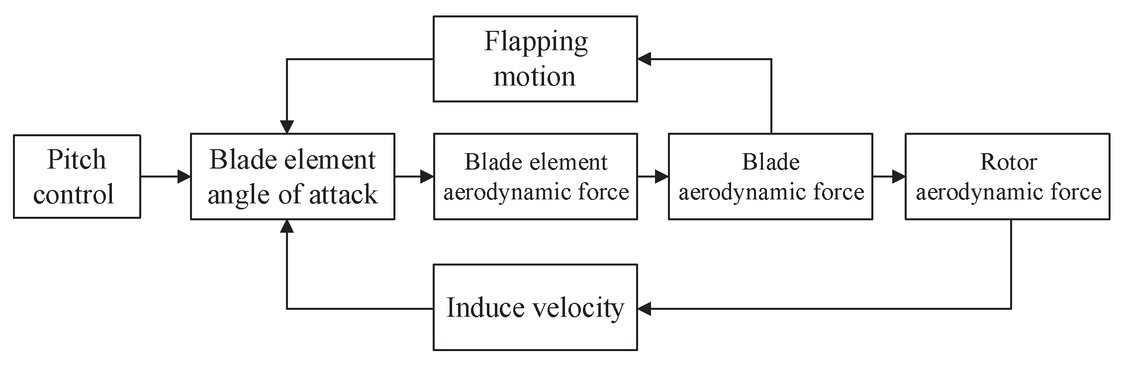
The main rotors are the most significant components of the tiltrotor aircraft and they need to be modeled accurately so that meaningful results can be obtained. The rotor unsteady dynamic characteristics are described
Figure 2.
The main rotors’ aeromechanic features in this paper are summarized as follows [
27,
28]:
(1) The rotor blades are centrally hinged and assumed to be rigid.
(2) Blade aerodynamic force computed by nonlinear, quasi-steady aerodynamics in table look-up form as functions of angle of attack and Mach number.
(3) The model is a three degree-of-freedom, finite-state rotor inflow model.
(4) The flapping angles are expressed in multiblade coordinates (MBC).
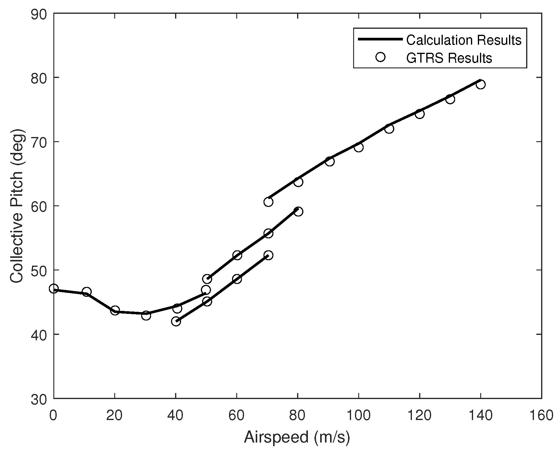
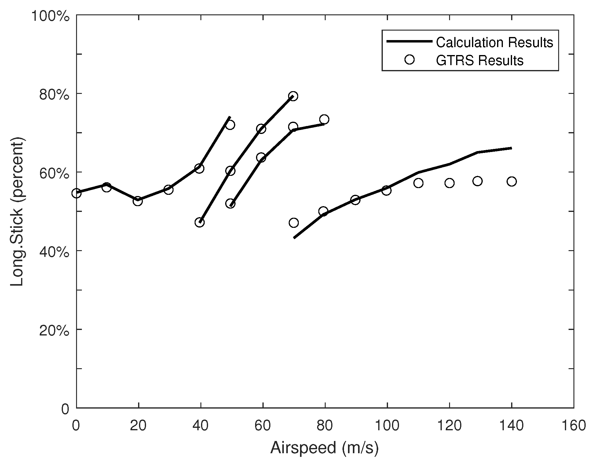
In the trim validation, the control inputs at different nacelle incidence angles are compared with simulation results from generic tiltrotor simulator (GTRS) reports.
Figure 3 and
Figure 4, respectively, show the comparison of collective pitch and longitudinal control. According to
Figure 3 and
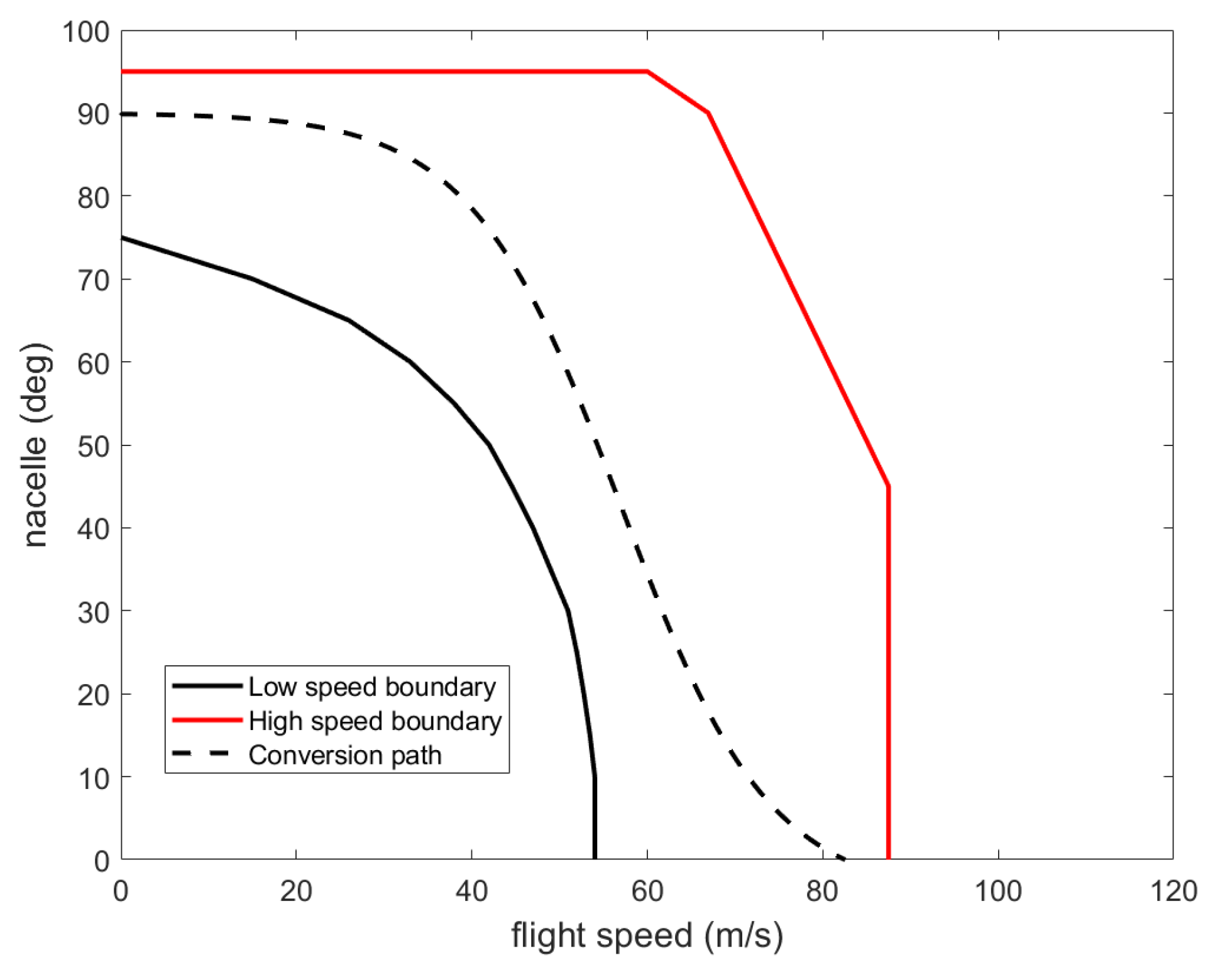
Figure 4, in helicopter mode, the variation trend of collective pitch is similar to that of the conventional helicopter. The collective pitch has the characteristic bucket profile as a function of flight speed. In airplane mode, the function of the rotor is providing forward pull force to overcome fuselage drag. That is to say, the wing is able to generate enough lift to overcome gravity. The collective pitch is much larger than that of the helicopter mode. In addition, longitudinal control input increases with speed in all flight modes. The conversion corridor is the unique flight envelope of the tiltrotor aircraft, defined as the constrained relationship between air speed and nacelle angle. The transition corridor is given in
Figure 5. The abscissa is the speed and the ordinate represents the inclination of the nacelles, each nacelle angle corresponding to a velocity range. As we can see from
Figure 5, the conversion path is completely in the conversion corridor, which meets the flight condition constraints of conversion mode. The flight test and GTRS are shown in
Table 2. As shown in
Table 2, the characteristics in helicopter mode of the eigenvalue distribution between calculation results in this paper and flight tests are very similar.
The tiltrotor is a symmetric vehicle, and the main motions of conversion flight are in the vertical plane. Therefore, only longitudinal dynamics need to be considered in this paper. The longitudinal model involves the attitude motion of the pitching angle and the translation on the
X axis and the
Z axis of the body.
where
and
are the forces caused by the rotor along the
and
axes,
and
are the forces caused by the other aircraft parts along the
and
axes and
is defined as pitching moment developed for the rotor.
The total forces and moments are obtained by summing up forces and moments from the rotors, the wing, the fuselage and the horizontal stabilizer. The wing/flap lift, drag and pitching moment coefficients are defined as functions of angle of attack, nacelle angle and flap setting. The fuselage aerodynamics are functions of angle of attack, and the horizontal stabilizer is modeled in a similar method.
The forces and moments from main rotors can be shown by:
where
T is the rotor thrust and
H is the horizontal force.
3. Control Law Design for the Conversion Flight Mode
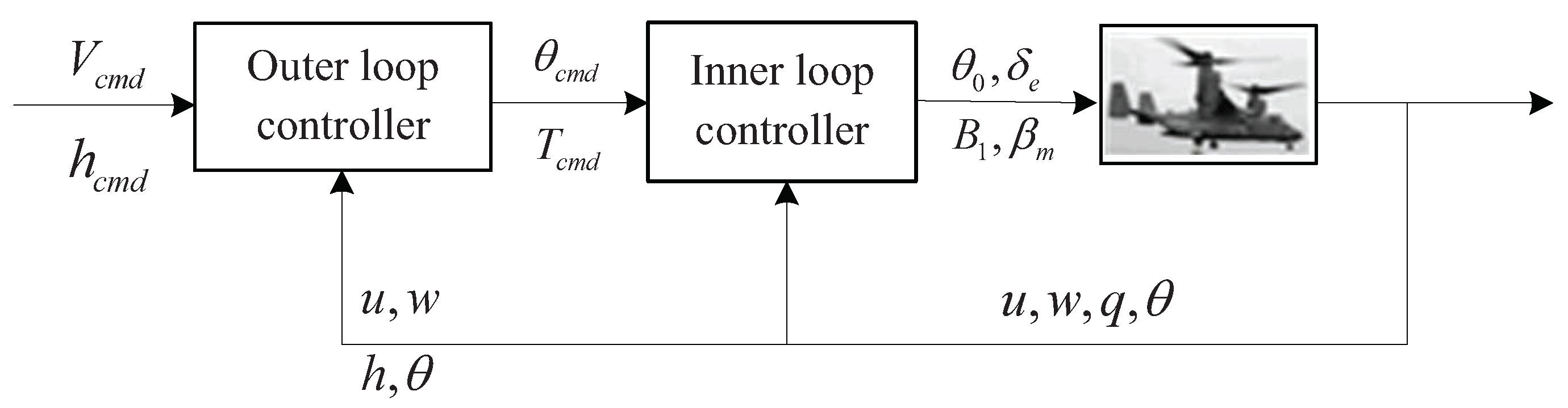
The flight control schemes for the tiltrotor aircraft have two time-scale separation architectures. They are composed of inner-loop SCAS for faster dynamics and outer-loop flight trajectory tracking control for slower dynamics.
Figure 6 shows the structure of the inner/outer loop of feedback controller.
The control objectives and the design technology of the inner loop and outer loop are different. The inputs of the outer loop are the altitude command and speed command , which generate the pitch angle command and rotor thrust command . Thus, the inner-loop variables to be controlled are the pitch angles and the rotor thrust, which are the inputs of the aircraft, viz., longitudinal stick input, collective pitch and elevator deflection.
The tiltrotor aircraft shows various dynamic characteristics when the flight modes change. As the nacelle rotates from a 0° angle in helicopter mode to a 90° angle in airplane mode, the flight mission changes from hovering with low speed to cruising with high speed.
In helicopter mode, pitching moment is controlled by adjusting the longitudinal cyclic pitch, which realizes the change of flight speed. The collective pitch simultaneously controls the engine throttles, thus realizing the control of flight altitude. However, in airplane mode, the elevators are activated by the pitch control inputs to realize the change of flight altitude and the collective controls activate the engine throttles to realize the change of forward speed.
In this section, the inner-loop control is designed first; then, the control allocation strategies are optimized; finally, the outer-loop control is used for flight trajectory tracking.
3.1. Inner-Loop Control Law Design in Conversion Flight Mode
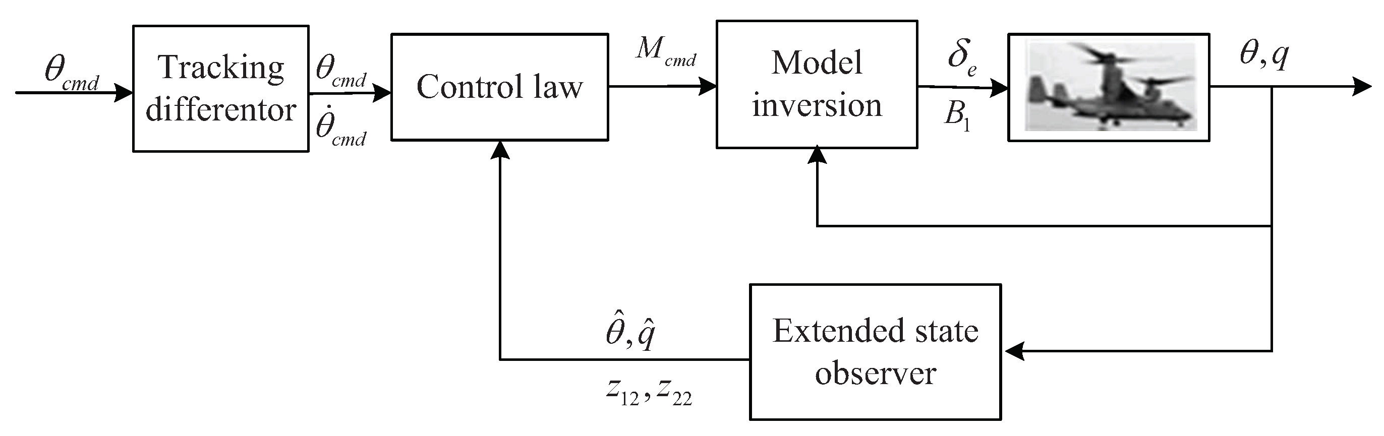
3.1.1. Attitude Control Law Design for the Inner Loop
In the inner-loop control, the input of the pitch attitude control system, as shown in
Figure 7, is pitch attitude command
, and the outputs are elevator deflection
and longitudinal cyclic pitch
. The weights, the longitudinal stick input and elevator, are obtained by the control allocation strategy, which will be given in the upcoming part.
The simplified longitudinal model is given by:
where
and
stand for the unknown lumped uncertainties, which include the internal parametric variation, model error and external disturbance acting on the corresponding channels. New system states are defined
and
. Then, the extended pitching channel model can be rewritten as:
To observe the pitch angle, the pitch acceleration and the disturbances in the pitching channel control system, a similar discretized ESO to that of the thrust control loop is designed.
The ESO can estimate the state and disturbance of a system without a precognition of the system. Disturbance is extended to a new state. Then, the system is defined as follows:
To obtain the disturbance
and
, a novel SMESO is designed as follows:
where
,
and
. The convergence of estimated error is proved in [
16].
3.1.2. Design of Tracking Differentiator
The tracking differentiator can track the attitude command and its differential as well as the angular rate command. It is designed as follows:
where
u is an input signal,
h is the sample time and
is the synthetic function for time optimal control. It is denoted by:
Therefore,
and
are the output and its differential. The output is shown in
Figure 7 when the input is a step signal.
3.1.3. Sliding Mode Controller
Based on the design of the SMESO, TD and dynamic surface control theory, the sliding mode control law is designed as follows:
where
and
are the estimated values of disturbances
and
,
denotes the vector of attitude command and
denotes the vector of angular rate command.
,
and
are chosen as positive definite matrices.
, and
The stability of the control law (
21) is proven as follows. The Lyapunov function is chosen as:
Equation (
22) is differentiated as follows:
According to Equations (
21) and (
23), it is known that
Because
and
are positive definite matrices, it is obvious that
,
is valid only when
. When
, we know that
From the Cauchy–Schwarz inequality, we know that
Because
and
, Equation (
26) gives
Above all, the stability of the control law is proven. Since the nonlinear item
, in the SMC may cause high-frequency chattering, it is replaced by the following function:
3.1.4. Control Allocation Strategy
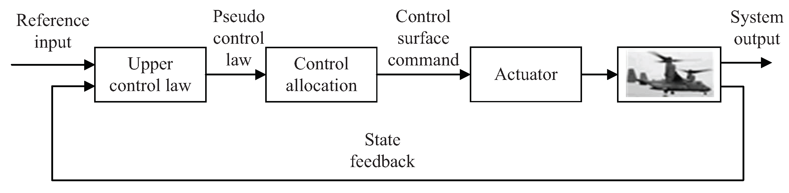
The control allocation strategy changes as the flight condition shifts from one mode to another. Therefore, the effector redundancy is managed by developing a control allocation module for distributing control effort among the available actuators. The block diagram of the overdrive control system based on control allocation is shown in
Figure 8.
After accepting the expected force or torque generated by the upper control law, the control distribution law is based on the minimization problem according to the constraints of each control surface:
where
and
represent the lower and upper bounds of the control surface, respectively,
is a function that executes the mapping from the executor to the upper control law and, in the case of attitude control law design for the inner loop,
represents
. In the inner-loop controller, the collective pitch only affects rotor thrust; therefore, the collective pitch is not considered in the control allocation strategy. The pitching moment needs to be distributed based on the weights of the longitudinal stick input and elevator involved according to nacelle angle. Pitching moment command
, which is the input to control pitching angle, is obtained by the control algorithm. Longitudinal stick command and elevator command can be obtained from their inverse models.
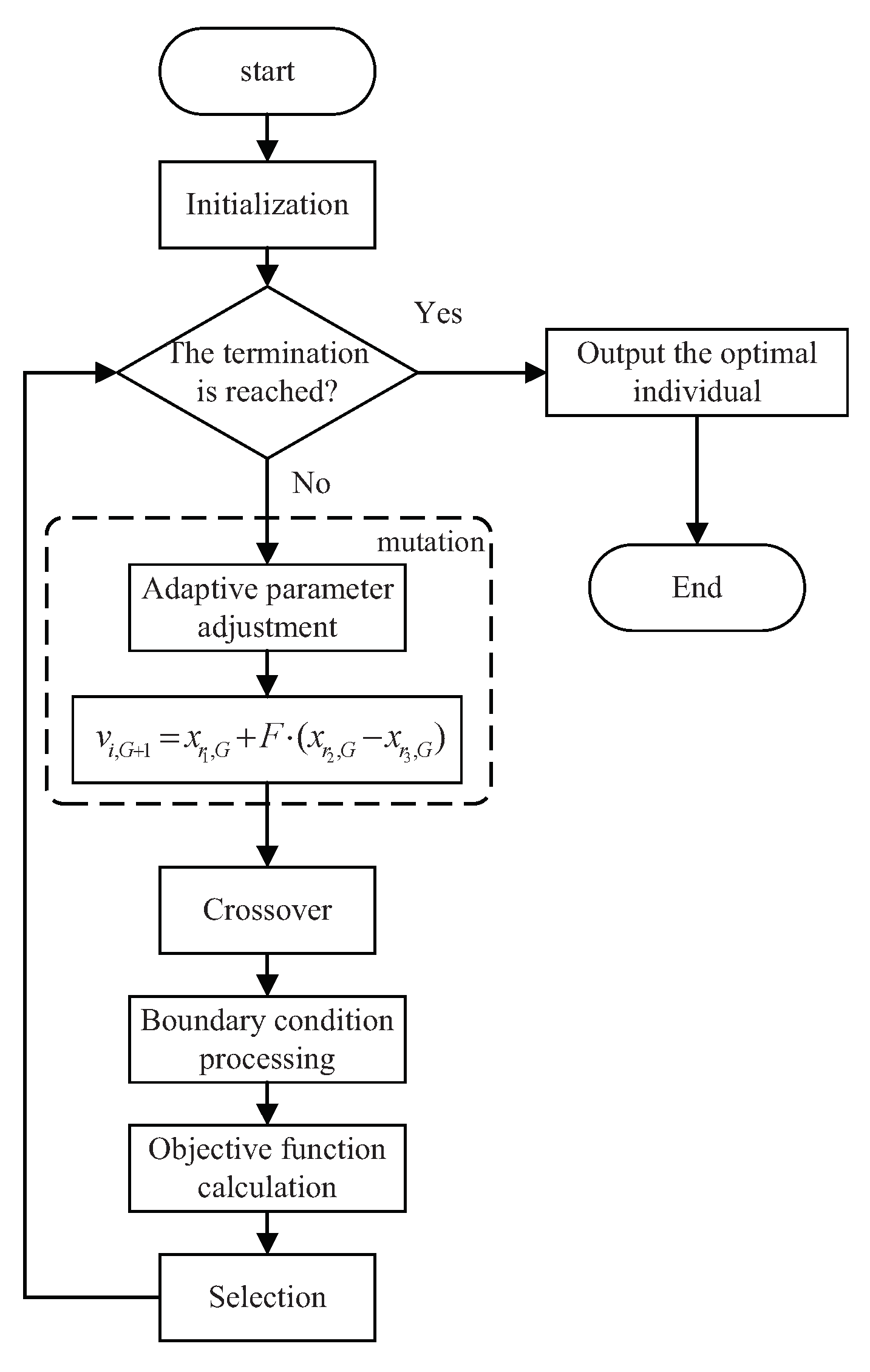
In this paper, an optimization strategy based on the adaptive differential evolution algorithm is used to design control allocation. The differential evolution algorithm is an intelligent optimization search algorithm generated by the cooperation and competition between individuals in a group. The operation steps of the basic differential evolution algorithm include initialization, mutation, crossover, selection and boundary condition processing. The process of solving optimization problems by the adaptive differential evolution algorithm is described below:
For
parameter vectors with dimensions being equal to
D, each individual is expressed as:
where
i represents the sequence of individuals in a population,
G is the evolution algebra and
is the size of the population. In differential evolution algorithms, it is generally assumed that all randomly initialized populations conform to a uniform probability distribution. Let the bounds of the parameter variable be
. Then, we have
where
and
represents a uniform random number between 0 and 1.
- (2)
Mutation
For each of the target vectors
, the vector of variation is generated by the following equation:
where
represents the mutation operator.
- (3)
Crossover
In order to increase the diversity of interference parameter vectors, the crossover operation is introduced, and then the test vector can be given by:
where
,
stands for the crossover operator.
- (4)
Selection
The optimal individual population is selected according to the fitness value.
- (5)
Boundary condition processing
For the problems of boundary constraints, it is necessary to ensure that the new generated individuals are in the feasible region. Then,
where
and
. The workflow of the adaptive differential evolution algorithm is shown in
Figure 9, and the objective function is
.
3.1.5. Inner-Loop Thrust Control Law Design in Conversion Flight Mode
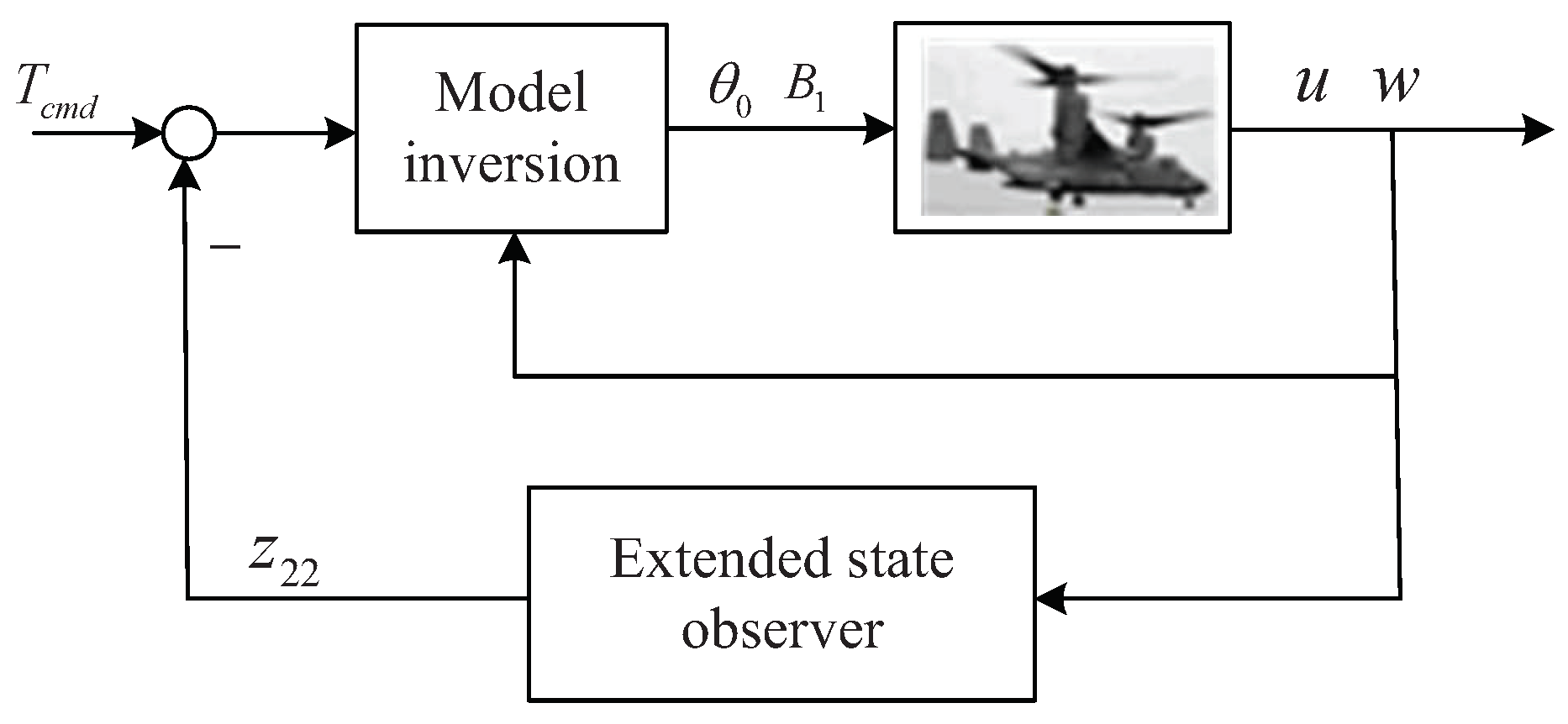
As the flight characteristics significantly vary during the transition process, the collective pitch is coupled with the pitch angle control and the longitudinal cyclic pitch is coupled with the thrust, as well. Using ADRC in the inner loop is an effective method for compensating the union of model error, coupled effects and external disturbance. The inner loop consists of pitch angle control and thrust control. The structure of thrust control is shown in
Figure 10.
The thrust coefficient
is:
Due to the coupled relation of collective pitch and longitudinal cyclic pitch and other interference terms, we have the thrust expression as in (
36):
Considering that the direction of thrust changes as the nacelle rotates, the force equation can be reformulated in the direction of thrust as in (
37):
where
d includes the disturbance and the model uncertainties.
Therefore, the acceleration along the rotor due to thrust is:
The disturbance term in (
38) is defined as a new system state. Then, the rotor thrust model can be rewritten as (
39):
To estimate the disturbance online, a discretized ESO is designed:
where virtual state
is the estimation of disturbance and
,
,
and
are positive constants.
According to the rotor thrust (
36), we can obtain the inverse model of rotor collective pitch by:
Therefore, the accurate collective pitch command can be obtained to ensure satisfied control performance of the tiltrotor aircraft.
3.2. Outer-Loop Control Law Design in Conversion Flight Mode
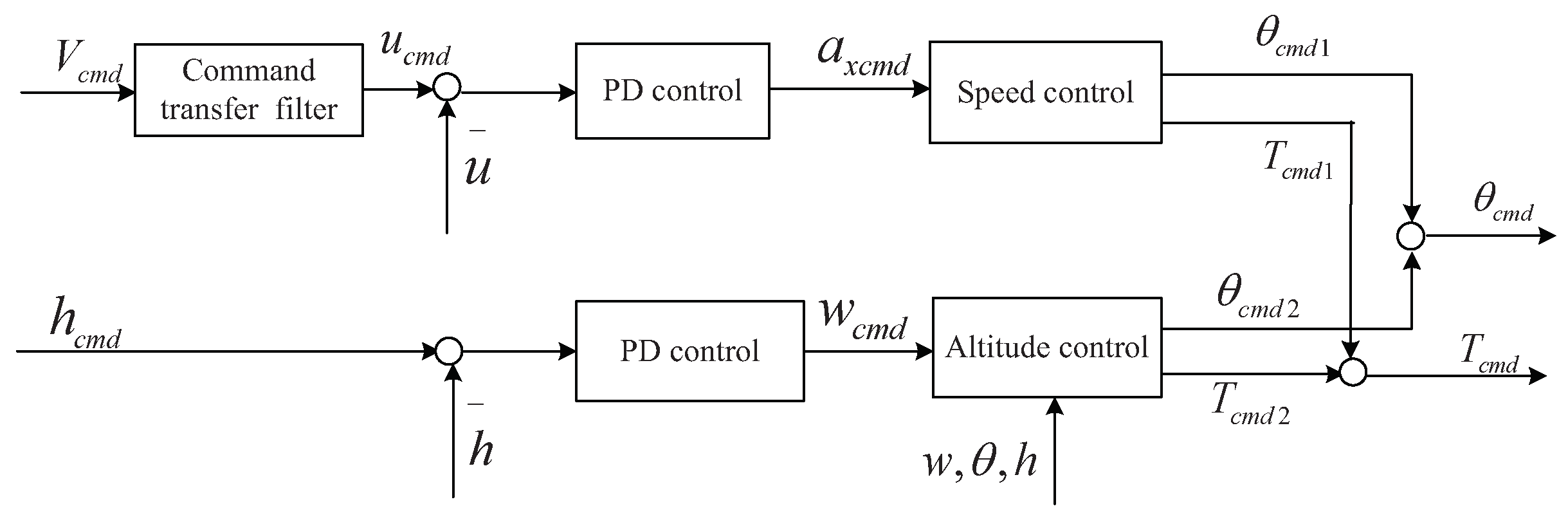
The structure of the outer loop of the longitudinal channel is shown by
Figure 11. The task of the outer loop is to control the speed and altitude based on ADRC by PD control.
is filtered and transformed to the coordinate system of the body through the command transfer-filter. The filtered output
is compared to measured values
u to yield tracking errors as the input of the PD controller. The output acceleration
is composed of two parts: one is the gravitational acceleration component
and another is produced by the force of the rotor. They are all along the longitudinal axis.
is given by:
The pitch angle and rotor thrust command yield as in (
45) and (
46) are:
where
is acceleration.
In altitude control, the function relation between flight altitude and speed is:
It should be noted that the lift generated by a tiltrotor aircraft is hard to estimate, so it would be difficult to give the reference input signal of the pitch angle at a constant altitude, especially in airplane-mode, the pitch angle of which having the characteristic of long period mode. Thus, an extended state observer is utilized to estimate pitch angle in altitude control.
The time derivative of altitude can be expressed as:
Equation (
48) can be rewritten as (
49) when the pitch angle is small.
where
d is a total disturbance.
Disturbance in (
49) can be defined as an extended state
, and let
. Thus, the altitude control subsystem can be formulated as:
For system (
50), the discretized ESO is designed as follows:
The expression of the function
is given by:
where
is a sign function,
is sampling period and
,
,
,
and
are positive constants designed to affect the estimation of the observer.
It can been proved that if the above parameters are properly selected, then the state estimation errors can converge to zero.
Then, pitch angle command and rotor thrust command in altitude control are given by:
Therefore, the outputs of the outer loop in
Figure 11 are given by:
4. Simulation Results
To analyze the properties of the control schemes, the simulations have been carried out and results are presented in this section.
In the simulation, the flap setting of the tiltrotor aircraft is adjusted with the change of flight speed during the conversion flight process. In helicopter mode, the flaps need to be extended to reduce the wing load consumption caused by the airflow downwash of the rotor. In airplane mode, the flaps need to be retracted to minimize the forward flight resistance at high-speed cruise.
The simulation result is shown in
Figure 12,
Figure 13,
Figure 14,
Figure 15,
Figure 16 and
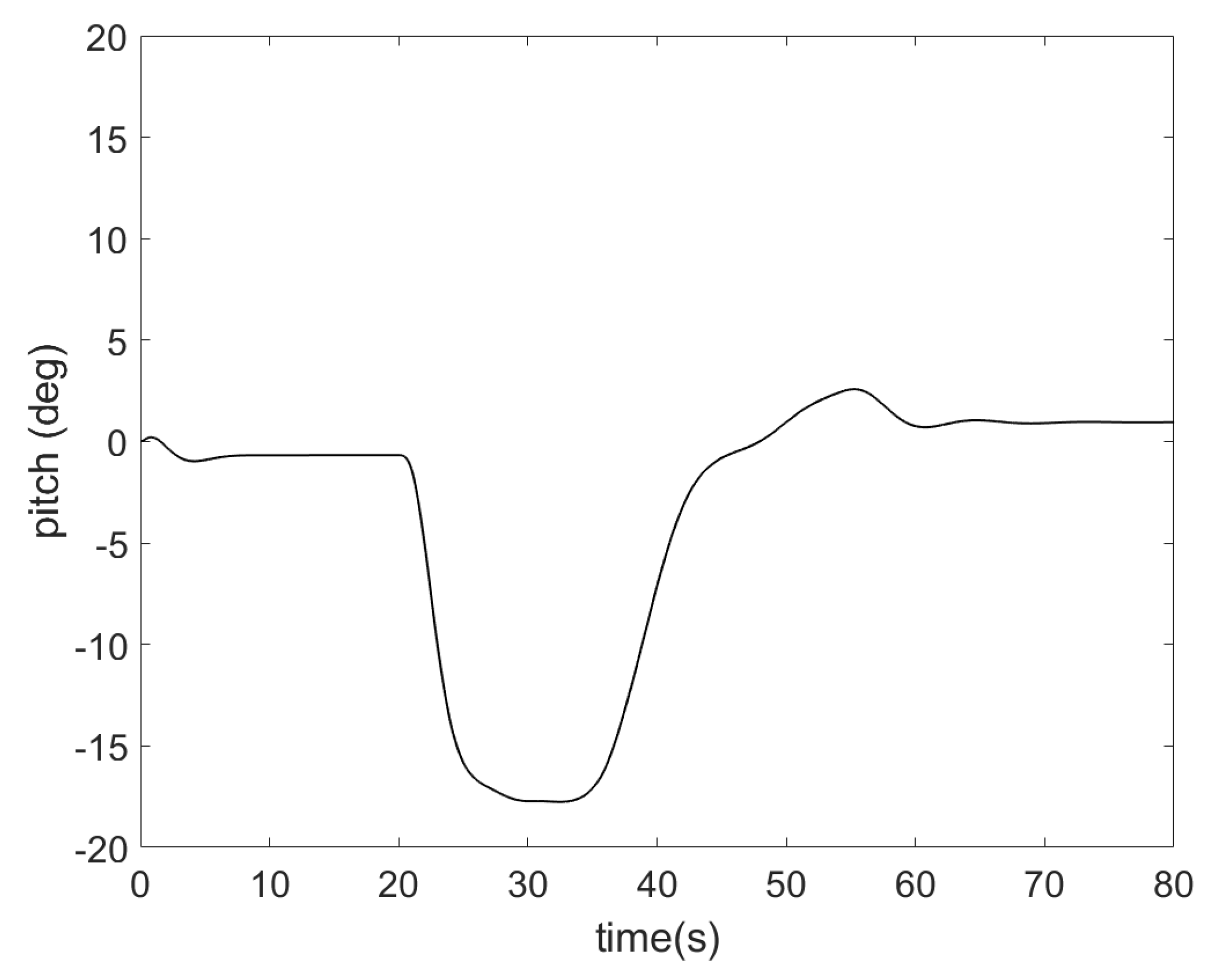
Figure 17. The pitch angle changes in the conversion model from helicopter to airplane are shown in
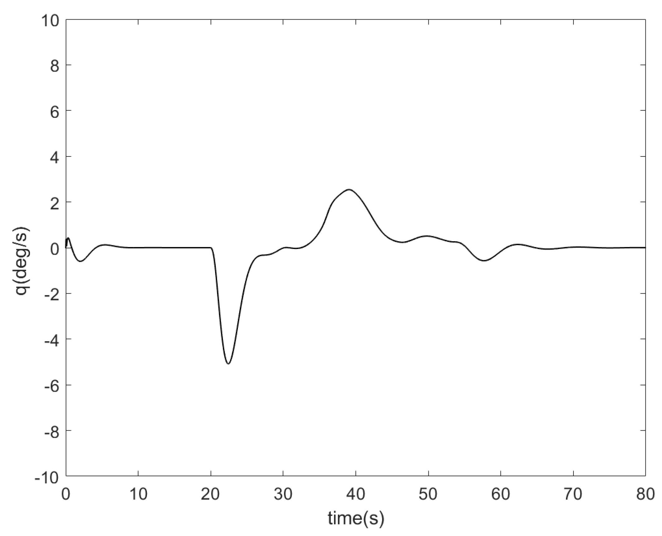
Figure 12. During the whole transition, the maximum pitch angle changes to about 17 deg, which was acceptable to the pilot. It can be seen from the
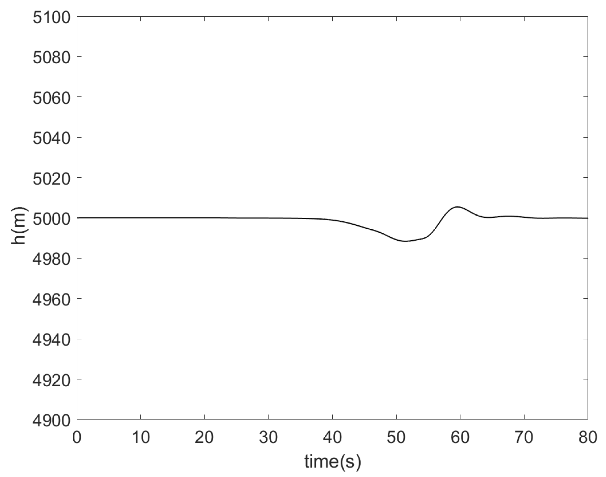
Figure 13 that the angular velocity changes smoothly. As can be seen from
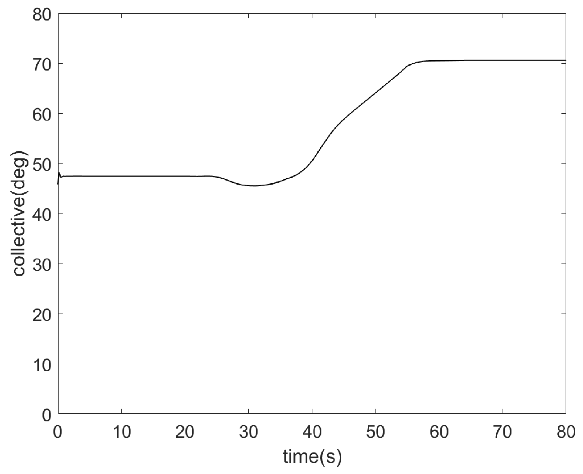
Figure 14, the height remains basically unchanged throughout the transition process, which is a sign of successful transition mode transformation. The change in the collective is shown in
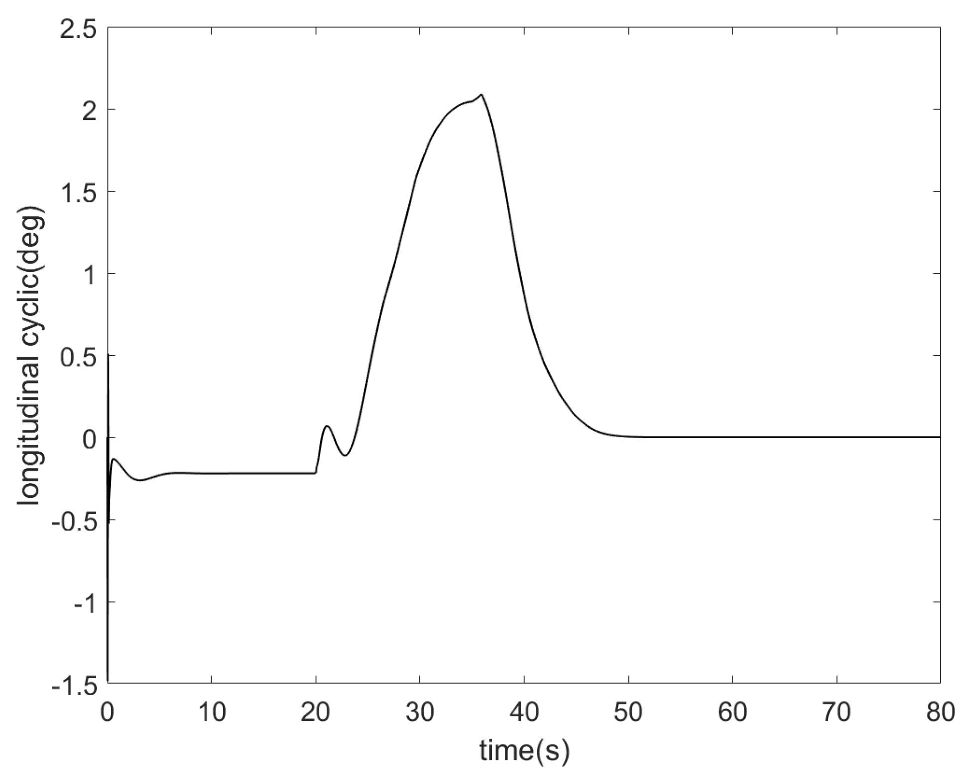
Figure 15. The collective is an increasing process.
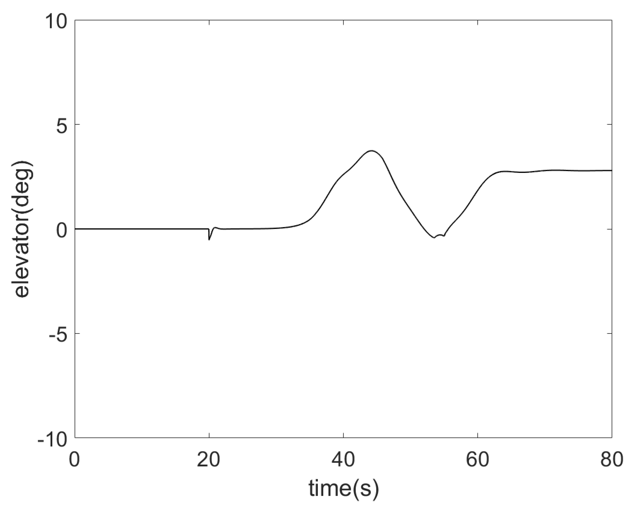
Figure 16 and
Figure 17 show the change rules of longitudinal cyclic and elevator, respectively. It can be concluded that the control allocation strategy designed in this paper is successful.


