Article

Hierarchical Optimization Algorithm and Applications of Spacecraft Trajectory Optimization

School of Astronautics, Beihang University, Beijing 102206, China
*
Author to whom correspondence should be addressed.
Aerospace 2022, 9(2), 81; https://doi.org/10.3390/aerospace9020081
Submission received: 23 November 2021 / Revised: 18 January 2022 / Accepted: 29 January 2022 / Published: 3 February 2022
(This article belongs to the Section Astronautics & Space Science)

Abstract

:
The pursuit of excellent performance in meta-heuristic algorithms has led to a myriad of extensive and profound research and achievements. Notably, many space mission planning problems are solved with the help of meta-heuristic algorithms, and relevant studies continue to appear. This paper introduces a hierarchical optimization frame in which two types of particles—B-particles and S-particles—synergistically search for the optima. Global exploration relies on B-particles, whose motional direction and step length are designed independently. S-particles are for fine local exploitation near the current best B-particle. Two specific algorithms are designed according to this frame. New variants of classical benchmark functions are used to better test the proposed algorithms. Furthermore, two spacecraft trajectory optimization problems, spacecraft multi-impulse orbit transfer and the pursuit-evasion game of two spacecraft, are employed to examine the applicability of the proposed algorithms. The simulation results indicate that the hierarchical optimization algorithms perform well on given trials and have great potential for space mission planning.

1. Introduction

In the last twenty years, the rapid development of meta-heuristic optimization algorithms has promoted the extraordinary progress of widespread engineering applications, including variable selection in chemical modeling [1], pattern recognition [2], path planning of UAVs [3], feature selection [4] and data clustering [5]. Doubtlessly, the powerful capabilities of parameter optimization are beneficial to space missions planning, such as spacecraft rendezvous trajectory optimization [6], interplanetary trajectories by multiple gravity-assist [7], agile satellite constellation design [8] and spacecraft attitude maneuver path planning [9]. In order to effectively apply the meta-heuristic algorithms to the space mission planning, on the one hand, constructing an appropriate optimization problem model is of vital importance. On the other hand, it is valuable to improve the performance of algorithms, which is the focus of this paper. Compared with traditional mathematical programming methods, meta-heuristic algorithms attract the attention of a large number of scholars due to four characteristics: simplicity, flexibility, derivation-free mechanism and local optima avoidance [10]. Relevant research can be divided into three types: proposing new optimization algorithms, improving existing algorithms and applying existing algorithms to practical problems. Apparently, new algorithms are most noteworthy for their new mechanisms to provide inspiration for other methods.
To design a highly applicable meta-heuristic algorithm, researchers have abstracted phenomena and laws in the real world into mathematical descriptions, from which a great number of algorithms were born. Genetic Algorithm (GA) [11] imitates Darwinian evolution theory and is a pioneer of multitudinous evolutionary optimization algorithms, including Evolutionary Programming (EP) [12] and Differential Evolution (DE) [13]. Typical mechanisms in this type of algorithm include selection, crossover and mutation, which have been extensively embedded in other algorithms to improve their performance [14]. To date, improved evolutionary algorithms are still studied by researcher [15]. The hybridization of evolutionary algorithms and local search operators produces the memetic algorithm (MA) [16], in which the local search is used to improve search efficiency. The efficiency and effectiveness of the local search mechanism depends on three principal components: the pivot rule, the iteration condition and the neighborhood generating function. The strategy of local search can be fixed or adaptive, according to the performance of multiple operators [17]. The primary characteristic of MA is the evolutionary operators used in global exploration, and multitudinous algorithms have been proposed to design and combine appropriate local search strategies to better solve the problems.
Individuals in evolutionary algorithms are relatively independent, and the connection depends only on crossover between individuals. Swarm intelligence (SI) optimization can strengthen and consolidate the connection. Particle Swarm Optimization (PSO) [18] is one of the most popular SI algorithms, which is inspired by the behavior of birds flocking in nature. In PSO, every particle makes decisions about its movement by self-cognition and social cognition. Self-cognition is the historical best position of a particle, and social cognition means the position of the current best particle. Improvement of PSO is proposed by many researchers to attempt to eradicate the shortcomings of premature convergence and lack of dynamicity [19], and to enlarge the applying scope [20]. A review of PSO was conducted by [21]. A mechanism of learning from the best particle has been introduced to many SI algorithms, such as Firefly Algorithm (FA) [22], Grey Wolf Optimizer (GWO) [10], Harris Hawk Optimization (HHO) [23], etc. For more detailed information about reviews on swarm intelligence and evolutionary algorithms, [24] is recommended. There are also many optimization algorithms designed according to physical phenomena and mathematical operations, including Simulated Annealing (SA) [25], Gravitational Search Algorithm (GSA) [26], Sine Cosine Algorithm (SCA) [27] and Arithmetic Optimization Algorithm (AOA) [28]. While there are already many optimization algorithms, there are still new optimization algorithms continually being proposed. The No Free Lunch (NFL) theorem is an explanation for this phenomenon [29], which proves that no algorithm is able to handle all problems well. Therefore, this motivated us to propose a new method for optimization.
The optimal solution for space mission planning problems is usually difficult to find, due to the complex landscape of the search space, which ultimately leads to algorithms obtaining suboptimal solutions. The reason is that the process of solution search has two phases: exploration for global search and exploitation for local search. Considering the contradiction between the two phases, existing algorithms usually switch from exploration to exploitation over the iterations, and strive to balance the ratio of two phases to increase the search efficiency. However, the algorithms pay heavy penalties for extricating from the vicinity of suboptimal solutions. If an algorithm can simultaneously perform both exploration and exploitation over the iterative search, the search efficiency will be improved. The goal of this paper is to solve this problem to a certain extent.
In this paper, a new swarm intelligence two-hierarchy optimization frame (HOF) is proposed. The core idea of HOF is the rational allocation of limited computing resources, namely the number of function evaluations. Motivated by the trends of the local search operations incorporated in memetic algorithms, we designed the HOF by endowing the best individual with additional function evaluations as a reward to enhance the search ability of the best individual compared with others. The strategy of HOF is to generate two types of particles, B-particle and S-particle, to search the variable space in two hierarchies, respectively. Therefore, the total number of function evaluations is determined according to the iteration numbers of two hierarchies, the B-particle number and the S-particle number. In the search of the first hierarchy, a certain number of B-particles explore the space iteratively. The motion direction and step length of B-particles are determined separately to improve the designability of algorithms and increase the exploration efficiency of B-particles. In each iteration of B-particles, the best B-particle has additional function evaluations provided by the local search of the second hierarchy, in which a certain number of S-particles iteratively exploit the neighborhood, and the best result is returned to update the position of the best B-particle. The number of function evaluations is a constant predefined and identical to the total number of generated S-particles. Two specific algorithms, HOA-1 and HOA-2, are designed based on HOF, and the difference lies in the local search methods of S-particles. In both algorithms, B-particles, except the best one, iteratively search the space by referring to the best two B-particles. In HOA-1, S-particles perform a pattern search by iteratively searching the space dimension by dimension, and the search step length in each dimension is a uniformly distributed random number with stepped decreasing bounds with the increase in the iteration number of first hierarchy. In each iteration of the second hierarchy, S-particles in HOA-2 are generated simultaneously based on a set of Gaussian distributions, which are iteratively updated according to the positions of the current best two function values.
To test the effectiveness of algorithms, the benchmark functions test is a popular method. However, some existing algorithms perform well in solving benchmark functions whose solutions are the origin of the search space, and an obvious performance degradation appears when the solutions deviate a little from the origin. Considering this unreasonable phenomenon, twenty-three variant benchmark functions are designed. In contrast to regular benchmark functions repeated solving, we set a random position deviation to the solution of the benchmark function, while keeping the minimum value invariant. Therefore, these variant benchmark functions were solved by the two proposed algorithms and seven existing algorithms repeatedly. Besides the benchmark functions test, two spacecraft trajectory optimization problems were solved by proposed algorithms and compared algorithms. The first problem was the spacecraft multi-impulse orbit transfer between two coplanar orbits, and the target was to find the optimal velocity impulse vectors and corresponding time. The second problem is the two-spacecraft pursuit-evasion game solved by the multiple shooting method, and the target is to find a set of appropriate costate variable initial values.
The rest of this paper is arranged as follows: Section 2 gives a statement about the optimization problem to be solved. Section 3 describes HOF and two algorithms systematically. The performance tests of proposed algorithms on benchmark functions and trajectory optimization problems are respectively presented in Section 4 and Section 5. The conclusion is given in Section 6 ultimately.

2. Optimization Problem Formulation

Optimization problems cover a wide range of subproblem types, which can be single-objective or multi-objective, unconstrained or constrained, static or dynamic. The focus of this work is to solve the static unconstrained single-objective optimization problem (SUSOP), since other types of problems can be studied by introducing more techniques and mechanisms into the achievement of SUSOP. Stochastic/heuristic optimization techniques have been extensively employed to handle optimization problems, and explicit reviews in [10,27] may help interested readers gain a comprehensive understanding of the development in this field.
This section gives a brief description and definition of the problem to be studied in the following work. Usually, a minimization problem is formulated to represent the optimization problem, as follows:
Minimize : f ( X ) X = ( x 1 , x 2 , , x N 1 , x N ) T l b i x i u b i ,   i = 1 , 2 , , N U b = ( u b 1 , u b 2 , , u b N ) T L b = ( l b 1 , l b 2 , , l b N ) T
where l b i and u b i are boundary values of the ith element of state variable X due to the restrictions on an N-dimension search space in numerical calculation. The continuity of function f means that a best solution must exist in the search space, even though the global optima may not be located in this space, especially for those problems in which it is difficult to stipulate the search space, for instance, when it is necessary to search for the initial values of costate variables in two-point boundary problem solving.
To find the best solution of the SUSOP, abundant algorithms have been proposed. Meta-heuristic algorithms are one kind of method quite popular over recent decades. A typical feature of meta-heuristics is the random factor, which leads meta-heuristics to receive different results so as to increase the probability of finding the optimal solution. A meta-heuristic algorithm (MHA) can be formulated as follows:
X * = M H A ( f ( X ) , X 0 , { P } )
where f ( X ) is the optimization function with a given search space, X 0 is the initial values, {P} is the parameter set including constant and varied parameters, and X * is the solution of f ( X ) obtained by MHA. The performance of MHA is significantly influenced by the values of {P}. However, the focus of this work is to design the search strategy, while the values of parameters are intuitively set and manually adjusted by the simulation results in the following paper.

3. Hierarchical Optimization Algorithm

The structure of HOF is outlined in this section. Subsequently, two specific algorithms, HOA-1 and HOA-2, are provided and their differences are discussed.

3.1. Hierarchical Optimization Frame

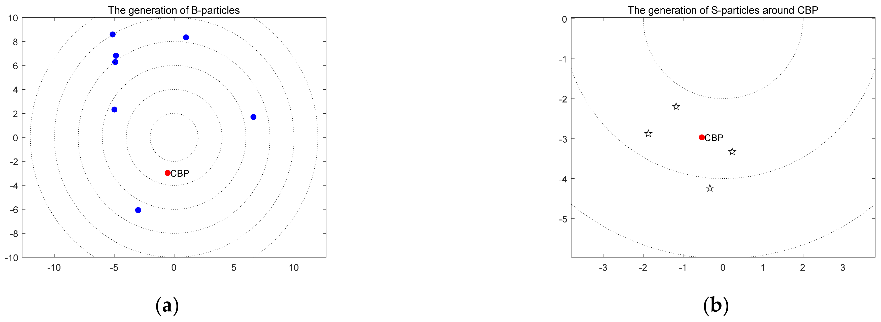
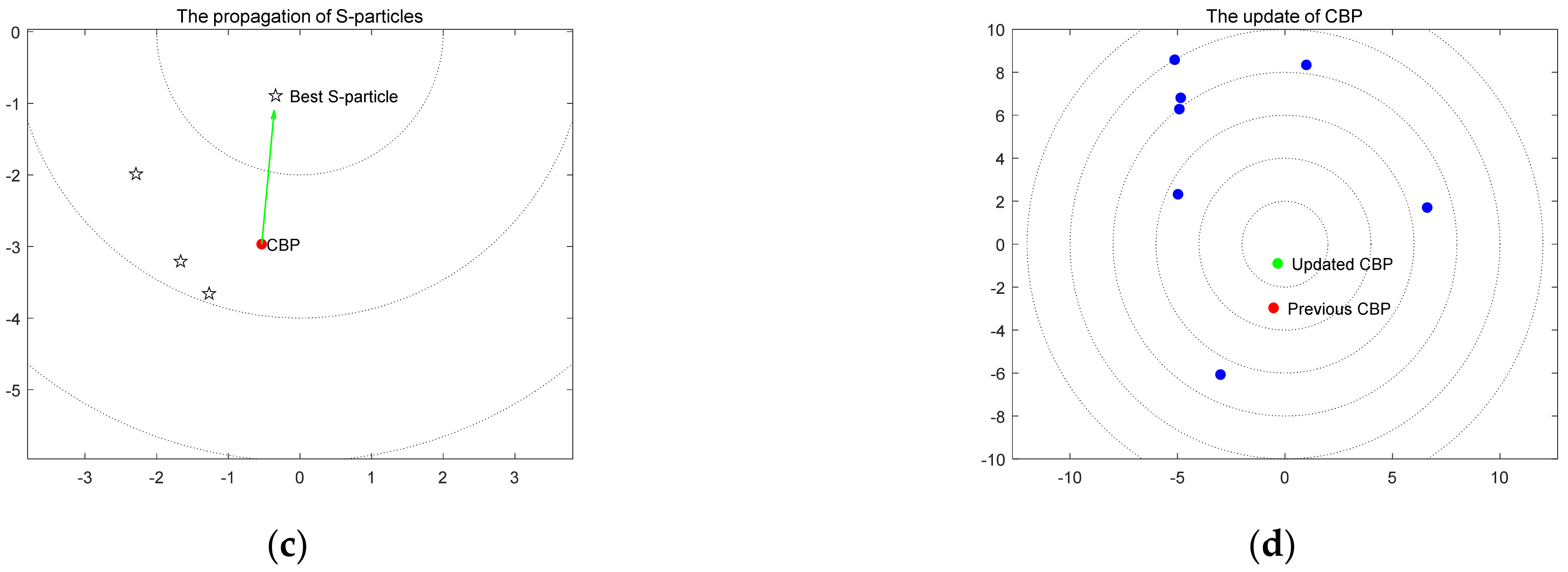
In this paper, we used particles to represent the individuals in SI algorithms. For SI algorithms, a popular idea is to use the position of the current best particle (CBP) to guide other particles’ motion, which makes the exploration and exploitation in the search space more effective and efficient. However, CBP itself seldom obtains benefit from this strategy. To alleviate this limitation, HOF was proposed to enhance the search ability of CBP by performing a local search and giving it additional function evaluations. HOF includes two hierarchies: H1 is the first hierarchy and H2 is the second hierarchy. In H1, a certain number of particles called B-particles are used to iteratively search for the global optimum. Therefore, the CBP in HOF is the current best B-particle. In each H1 iteration, B-particles cooperate to iteratively update their positions based on the current information of search results. Generally, only one function evaluation is conducted to complete the position update of each B-particle except CBP, whose position update depends on the local search of H2 iterations and requires more function evaluations. In H2, particles of another type called S-particles, initially distributed in the neighborhood of CBP, are assigned to iteratively exploit the space. After a predefined constant number of S-particles are randomly generated, the position of the best S-particle becomes the updated position of CBP based on the greedy strategy. The iterations of two hierarchies are executed in turn until the maximum number of H1 iterations is reached. Note that B-particles converge as the H1 iterative search progresses, while S-particles dispersedly exploit the local space from the initial position of CBP. I b and I s are the maximum number of iterations in H1 and H2, which means that I s times H2 iterations proceed after each H1 iteration, and the stopping criterion is I b times H1 iterations have been performed. The total number of function evaluations is determined according to the iteration numbers I b and I s , the B-particles number and the S-particles number. The whole frame is modularized and illustrated by Figure 1, in which the orange blocks represent adjustable sub-algorithms. A 2-D sphere function was used to show the CBP’s update process in one H1 iteration with its subsidiary H2 iterations. In Figure 2, Figure 2a shows the positions of eight B-particles, in which the CBP is represented by a red marker, while other B-particles are blue markers. Four S-particles, marked by pentagrams, were used to perform the local search in the neighborhood of the CBP, and their initial positions and final positions are respectively given in Figure 2b,c. The best S-particle was selected to update the CBP’s position after H2 iterations, and is denoted by the green marker in Figure 2d.
There is no specific formula given in the flowchart in Figure 1. To design specific algorithms, we designed an iterative method for B-particles used in this paper, while other methods are also applicable. In H1, we culled the best two B-particles in each iteration and set them as two leaders, L1 and L2, to guide the motion of other B-particles in the next iteration, except for L1’s position, which was determined by the result of H2 iterations. Each SI algorithm has its own way of deriving particle propagation, including two aspects, the direction and the step length. The velocity computation of PSO provides a particle’s motional direction and step length simultaneously. In comparison, the direction and step length of bacteria are computed respectively in Bacterial Foraging Algorithm [30], in which the direction is a unit vector randomly produced in the searching space, and the step length is a small predetermined value to meet search accuracy. Both algorithms have respective advantages and limitations, which inspired us to separate the determination of searching direction and step length to strengthen the algorithm’s flexibility and adaptability for different optimization problems.
Since the search direction and step length are calculated respectively, we used positions of L1 and L2 to derive a particle’s direction update formula by
D i n = c 1 ( L 1 n B i n ) + c 2 ( L 2 n B i n ) c 1 ( L 1 n B i n ) + c 2 ( L 2 n B i n )
where B i n indicates ith B-particle’s position in nth iteration in H1, L 1 n and L 2 n represent the positions of L1 and L2 in nth iteration respectively and the parameters c 1 and c 2 control the weights of L1 and L2 to B i n . The symbol · means the Euclidean norm of a vector. With the inconsistency of L1 and L2, the denominator of D i n is always larger than 0, which averts the singularity. Assuming L 1 n exerts more influence on B i n than L 2 n , we set c 1 > c 2 > 0 . The step length of B i n is given by
d e l t a B i n = α ( L 1 n B i n + L 2 n B i n ) / 2
where α is the step ecoefficiency between 0 and 1 to directly tune the searching range of B i n . In total, the updating equation of B i n in H1 iteration is constructed as follows:
B i n + 1 = B i n + d e l t a B i n D i n
note that the update mechanism of B-particles is deterministic, due to the constant values of c 1 , c 2 and α , which is not best, but effective. Further study on the autonomous adjustment of these parameters can be conducted by introducing randomness or adaptive laws.
L 1 n is actually the position of CBP in nth H1 iteration. Different ways to generate and update S-particles can construct many specific algorithms, one of which may better solve the focused problem. Two hierarchical optimization algorithms are introduced in the next subsection, and their difference lies in the local search method of S-particles.

3.2. Two Hierarchical Optimization Algorithms

Considering the performance differences caused by the different searching methods of S-particles, two hierarchical optimization algorithms, HOA-1 and HOA-2, are proposed to validate the effectiveness of HOF.

3.2.1. Formula of HOA-1

The searching method of S-particles can be divided into two steps: initialization and iterative update. The initialization is to determine the spatial domain and the position distribution law. The first step is to set a spatial domain of initial S-particle positions. A gradually shrinking domain makes a fine effect, because S-particles are used to search the neighborhood of CBP. In order to simplify the algorithm, we designed a function to control the boundary of this domain in Equation (6).
d e l t a S n = ( U b L b ) F ( n / T ) , n = 1 , 2 , , I b
where F ( ) is an operator to tune the range of d e l t a S n in nth H1 iterations, U b and L b are the boundary of the search space defined by (1), and T is a parameter to control the phased variation of search precision. In HOA-1, F ( ) is defined in (7).
F ( n / T ) = 10 n / T c
The symbol indicates rounding down the variable. This function means the domain stays invariant for T times H1 iterations, and shrinks to one tenth in the next T iterations, and c is a constant used to determine the initial search precision. Generally speaking, we suppose that a better position exists within a hypercube centered on CBP, and take d e l t a S n to set the length of its edges.
In HOA-1, the number of S-particles is equal to the dimension N of the problem to be solved, which results from the idea that changing the value of CBP’s position dimension by dimension serves to precisely search the space around CBP.
In H2 iterating process, the reference point P r is used to update the positions of S-particles, and the initial P r is the CBP of the B-particles in the current H1 iteration. Once a better position is found, it becomes the new P r of the next H2 iteration. Let S j m be the position of jth S-particle in mth H2 iteration. The updating equation of S j m is constructed as follows:
S j m = P r + r s I N , j d e l t a S n ( j ) , m = 1 , 2 , , I s
where I N , j is the jth column vector of a N-order identity matrix I N , d e l t a S n ( j ) is the jth element of d e l t a S n , and r s is a random number uniformly distributed in the interval of [–1,1]. After H2 iterations, the final P r is output to renew the position of CBP if its function value is smaller. The HOA-1 algorithm is summarized in Algorithm 1.
Algorithm 1 Pseudo code of HOA-1.
Generate initial Bi1 (i = 1, 2, …, p)
Calculate the fitness of each B-particle f(Bi1)
Choose L1 and L2
Starting H1 iterations:
while 1 (n < Ib)
for 1 Bin
  if 1 Bin doesn’t equal L1n
  Update the position by (5)
  else
  Starting H2 iterations:
  Input CBP’s position as Pr and fitness as fr and deltaSn by (6)
  while 2 (m < Is)
   for 2 Sjm(j = 1, 2, …, N)
    Generate Sjm by (8)
   if 2 f(Sim) < fr
   Pr = Sim 
   end if 2
   end for 2
  end while 2
  Output Pr as CBP’s updating position
end if 1
  end for 1
  Update L1 and L2 according to f(Bin+1)
end while 1
return the final L1

3.2.2. Formula of HOA-2

In HOA-1, the way S-particles search for a better solution is by changing only one element of P r in a given domain to generate a new S-particle that is uniformly distributed in the hypercube. To design a different search strategy, a new algorithm HOA-2 is proposed in which the number of S-particles can be specified arbitrarily, every element of each S-particle is obtained from a Gaussian distribution, and all elements are changed simultaneously. To determine a suitable Gaussian distribution, the mean value μ and the standard deviation σ should be defined. Thus, the positions of L1 and L2 are input to the H2 optimization, and μ and σ can be given as follows:
μ n 1 = L 1 n σ n 1 = a b s ( L 1 n L 2 n )
where μ n 1 and σ n 1 represent the first μ and σ in the H2 optimization of nth H1 iteration, respectively. The operator a b s ( ) is used to replace all elements of the vector with their absolute values. This specification stems from the assumption a better position exists closer to L1 than L2. Given that the range of this parameter setting is sometimes too large, another specification in Equation (10) is proposed, which is also subject to the above assumption.
μ n 1 = ( 2 L 1 n + L 2 n ) / 3 σ n 1 = a b s ( L 1 n L 2 n ) / 3
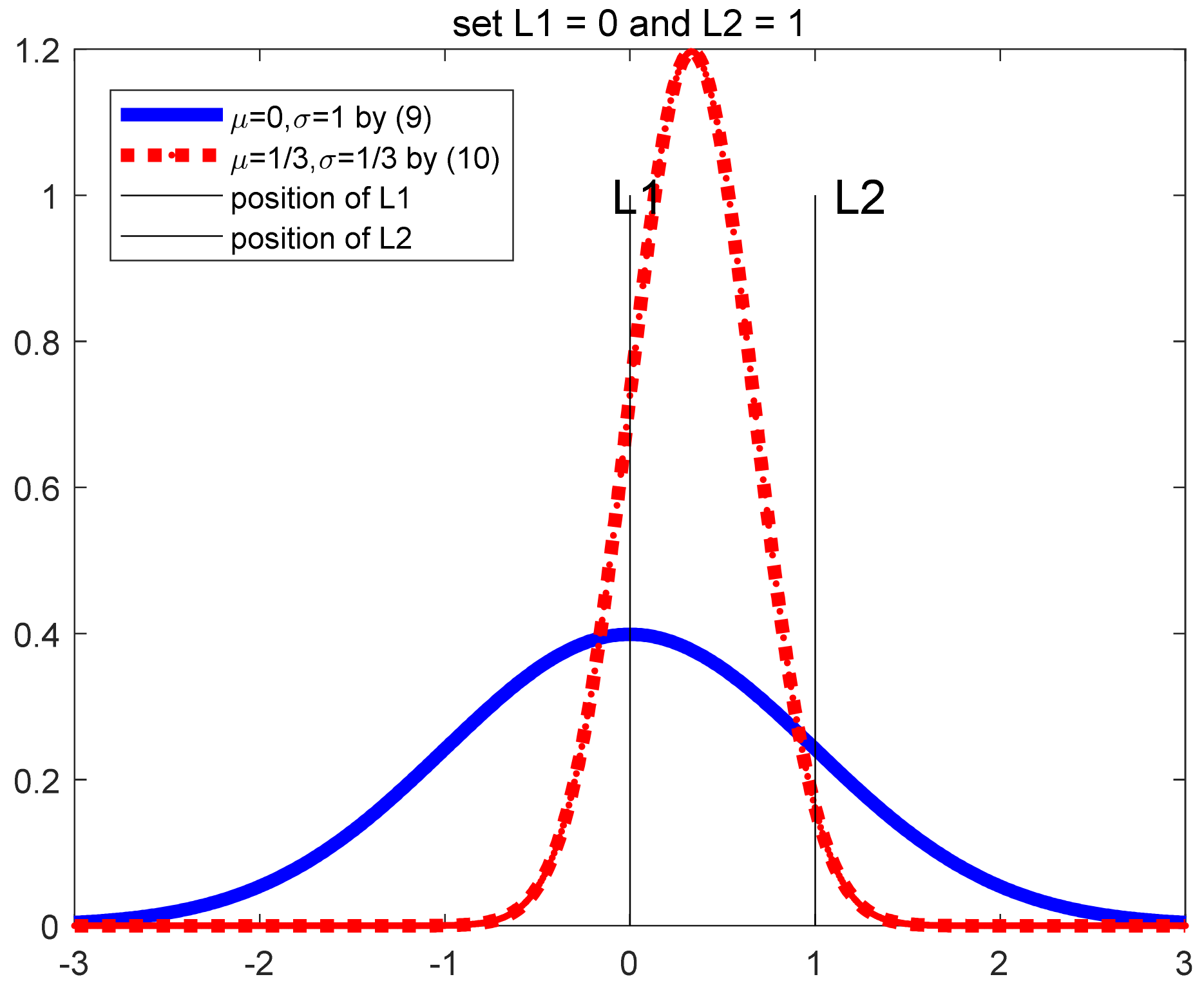
The difference between Equations (9) and (10) is illustrated in Figure 3, in which the curves are the probability distribution density functions of two ways. It shows the interval constrained by Equation (9) is obviously larger. Due to the high probability of the generation of new S-particles between L1 and L2 by using Equation (10), this specification is preferred when the best solution is encircled by S-particles.
To guarantee the validity of this estimation for better solutions, μ and σ are updated after every H2 iteration, which leads to the necessity of selecting and updating the best two S-particles, namely SL1 and SL2. Using SL1 and SL2 to severally replace L1 and L2 in Equations (9) or (10) can update μ and σ in each H2 iteration.
When the iterations in H1 proceed, if no other B-particle takes over these two particles, the difference between L1 and L2 becomes small, which makes the search space in H2 too narrow for S-particles to help CBP find a better position. With that in mind, a lower bound for σ is introduced to prevent S particles from being limited to a cramped space search. As with the restriction on d e l t a S n , Equation (11) gives the definition of σ and σ min .
σ min = ( U b L b ) F ( n / T ) , σ n m = a b s ( S L 1 m S L 2 m ) , a b s ( S L 1 m S L 2 m ) σ min σ min ,   else
where σ n m is σ in mth H2 iteration of nth H1 iteration, and S L 1 m and S L 2 m are positions of SL1 and SL2 in mth H2 iteration, respectively. Therefore, based on the setting of μ and σ in Equation (9), the updating equation of jth S-particle S j m in mth H2 iteration is constructed as follows:
S j ,   k m + 1 = Z k , Z k ~ N ( S L 1 k m , σ n m ( k ) )
where the subscript k means kth element of a vector and σ n m ( k ) is kth element of σ n m . Likewise, the setting of μ and σ based on Equation (10) can be derived, but is omitted here. The HOA-2 algorithm is summarized in Algorithm 2. To maintain the relative independence between H1 and H2, only SL1’s final position is output to update CBP’s position.
Algorithm 2 Pseudo code of HOA-2.
Generate initial Bi1 (i = 1, 2, …, p)
Calculate the fitness of each B-particle f(Bi1)
Choose L1 and L2
Starting H1 iterations:
while 1 (n < Ib)
  for 1 Bin 
   if 1 Bin does not equal L1n
  Update the position by (5)
else 
  Starting H2 iterations:
  Input the position and fitness of L1 and L2
  while 2 (m < Is)
   for 2 Sjm(j = 1, 2, …, q)
   Generate Sjm by (12)
   Update the position and fitness of SL1 and SL2
   Update μ and σ by (9) and (11).
  end for 2 
  end while 2
  Output SL1q as CBP’s updating position
end if 1 
  end for 1
  Update L1 and L2 according to f(Bin+1)
end while 1
return the final L1
HOA-1 and HOA-2 share the same H1 and differ from the search mechanism in H2, which manifests more optimization algorithms that can be proposed based on HOF. By introducing more mechanisms into HOF, such as evolutionary operators, simulated annealing mechanism and other effective mechanisms, a new algorithm with better performance can be accomplished.

3.3. Comparison with Other Algorithms

The concept of hierarchical optimization has been used in algorithm design and some results have been employed in single-objective optimization and multi-objective optimization. In [31], a hierarchical algorithm (HGA-PSO) was developed to construct two-layer optimization, in which the bottom layer, responsible for exploration, is based on GA, and the top layer, for exploitation, adopts PSO. The bottom layer includes many subgroups searching for the best solution independently. After each iteration in the bottom layer, some excellent individuals of every subgroup are brought together to form a new group to continue cooperative search in the top layer. Until the termination conditions are met, k individuals are selected randomly from the top layer to substitute random k individuals of every subgroup in the bottom layer before the next iteration starts. An external archive is established to store the results of the top layer search, and subgroups choose k individuals from the archive [32], which eliminates the negative influence of initialization and randomness of individuals in the top layer by outputting the final solution from the archive. Compared with the hierarchical optimization methods mentioned above, the HOF is based on a competition mechanism, which is analyzed in detail in Section 4.2.2 through simulation examples, instead of combining the best individuals from multiple subgroups to conduct a cooperative optimization. In [33], a multiagent collaborative search (MACS) method was proposed for local exploration of the subdomain generated by the branching method. Multiple agents were generated in the given subdomain and used to explore this subdomain by elaborate collaboration mechanisms. Afterwards, MACS was further developed based on a combination of Tchebycheff scalarization and Pareto dominance to solve multi-objective optimization problems [34]. Compared with MACS, the exploitation of S-particles around CBP is quite different. The most obvious difference is that S-particles locally search the space around CBP independently, while strong information interaction exists between agents in MACS. Also, a search subdomain is firstly determined, and then the population of agents is introduced and updated to search this invariant subdomain, while the local search space of S-particles varies with the position update of the current optimal solution.
Regarding the H2 optimization as the local search of H1 optimization, the frame of HOF is similar to memetic algorithms. Therefore, a further comparison of two proposed algorithms and existing algorithms is conducted from the point of view of the local search. An adaptive gradient descent-based local search was introduced in MA [35], in which the numbers of individuals considered in local search, the search steps and iterations decreased linearly during the iterations. However, the gradient calculation requires additional function evaluation to generate a new individual, which leads to the important task of determining the ratio of the function evaluations of gradient calculation to the total evaluation number. In HOA-1 and HOA-2, the local search of S-particles proceeds without gradient information, and accordingly, once function evaluation occurs when generating a new S-particle. The local search mechanism of HOA-1 can be classified as a pattern search method with random factors. The stepped decreasing upper bound of iterative step length of S-particles in each dimension is related to the iteration number of H1, and differentiates HOA-1 from other local pattern search methods, for example, the memetic algorithm combining PSO and pattern search refinement [36], and multi- coordinate search [37]. This stepped decreasing mechanism of search step guarantees the search ability of CBP, even if all B-particles converge in the early iterations of H1 and avoids the local minima.
Another point worth demonstration concerns the Gaussian distribution used in HOA-2. Kennedy proposed a Bare Bones Particle Swarms Optimization (BBPSO) in 2003 [38], in which every particle’s position update is obtained by the Gaussian distribution defined by the best particle position and its historical optimal position. Then, many researchers improved the mechanism of Gaussian distribution parameter setting to increase its searching efficiency [39,40]. In these algorithms, the weight of best individual in defining the Gaussian distribution parameters is identical to other individuals, due to the balance of exploration and exploitation during the iterations. In HOA-2, the weight of L1 or SL1 is determinately bigger than that of L2 or SL2, because it adopts the hypothesis that the solution is closer to the best particle than other particles. Understandably, this hypothesis leads to closer distances between sampled particles and the best particle, and thus causes the premature convergence. Therefore, this hypothesis has a negative effect on the exploration and is rejected by existing algorithms. However, only the best one of sampled S-particles is selected to update the position of the CBP, and other S-particles have no influence on the iterative exploration of B-particles, which allows an increase in the weight of the best particle. In HOA-2, the S-particles are simultaneously sampled based on the same set of Gaussian distributions in each H2 iteration, and these Gaussian distributions are updated according to the positions of two best S-particles Sl1 and SL2. However, each particle in BBPSO has its own set of Gaussian distributions, which means that only one particle is sampled based on these distribution functions. The multiple sampling based on the Gaussian distributions can better exploit the neighborhood of the best particle, while the randomness of single sampling brings a negative effect to the local search. The local search methods based on covariance matrix adaption also utilize multiple dimension Gaussian distribution to describe the sampling subdomain around the center of selected individuals [41]. However, this type of algorithm emphasizes the adaptive laws of the covariance matrix and step size, without considering the weights of dominant individuals.

4. Experiments on Benchmark Functions

In this section, twenty-three benchmark functions are used to validate the performance of HOA-1 and HOA-2 compared with other optimization algorithms. Then, analysis and discussion about the results are elucidated.

4.1. Explanations of Performance Test

For comprehensive inspection of optimization algorithms, twenty-three benchmark functions, which consist of three types of functions—unimodal, multimodal and fixed-dimension multimodal—were utilized in [10]. To better examine the performance of proposed HOA-1 and HOA-2, we designed variants of these twenty-three benchmark functions instead of directly using them to testify the overall effectiveness. The origin benchmark functions are listed in Table A1, Table A2 and Table A3 in Appendix A. We introduced skills of variable substitution to shift the theoretical solution of each benchmark function in the searching space, while keeping the minima unchanged. The variable substitution can be expressed as x i = y i r i , where r i is a random value in ( 19 u b i + 21 l b i ) / 40 , ( 21 u b i + 19 l b i ) / 40 which covers 1/20 of the range of ith dimension search space. Taking F1 sphere function as an example, the actual fitness function is i = 1 30 y i r i 2 , the range of each dimension is still [–100, 100], and r i is a uniformly distributed constant in [–5,5], which means the extreme point is no longer the coordinate origin but a random point near the origin. Solving the minima of F1 function repeatedly, the theoretical value is always 0, while the position is R = r 1 , , r 30 T , which is determined by the results of random sampling before the optimization starts. In this way, the efficacy of algorithms emerges more clearly.
In contrast to the proposed algorithms, seven algorithms were introduced as comparison algorithms, including three classical algorithms: GA, DE and PSO, and four recently proposed algorithms: GWO, Butterfly Optimization Algorithm (BOA) [42], HHO and AOA. The parameters of these algorithms are defined in Table 1. The numbers of iterations Imax of all these contrastive algorithms were all set to 500, and the population size was 30. Since two hierarchies exist in HOA-1 and HOA-2, we set I b to 100 and I s to 4 for the sake of fairness, which guarantees a smaller number of function evaluations in HOA-1 and HOA-2 than in those of the compared algorithms. Because different benchmark functions require different search precision, the parameter T in HOA-1 and HOA-2 is defined correspondingly.
These algorithms were executed 30 times to solve each benchmark function on a laptop with an Intel(R) Core (TM) i7-10510U CPU at 1.8 GHz and 16.0 GB of RAM. All these algorithms are coded in MATLAB R2020a.

4.2. Results and Discussion

4.2.1. The Performance

The results of previous experiments are arranged meticulously, and the data are displayed in Table 2, Table 3 and Table 4, in which the best results obtained by nine algorithms for each benchmark function are presented in bold. In these three tables, B, A and S respectively stand for the best result, the average value and the standard deviation. The results of benchmark function test are given in Table 2, Table 3 and Table 4, in which the minimum values of these benchmark functions are bold. In the unimodal benchmark functions test, HOA-1 and HHO both found the best solution of three of the seven functions, and showed outstanding exploitation ability, according to Table 2. Furthermore, the results of the multimodal functions test in Table 3 illustrate that the exploration ability of HOA-1 is superior to other algorithms. For local minima avoidance, the data in Table 4 demonstrate that all these algorithms performed similarly, while HOA-1, DE and PSO had a weak advantage on the others. To statistically display the performance of tested algorithms, the Friedman test [43] was used to reflect the performance, and the result is listed in Table 5, which proves the advantage of HOA-1 over other algorithms. The p-value of the Friedman test was 8.8089−15, suggesting the existence of significant differences among the tested algorithms. Generally, HOA-1 outperformed other algorithms in the benchmark functions tests. Compared with HOA-1, HOA-2 performed better in F15 than the others. However, it should be noted that HOA-2 is also an effective algorithm, because the mean rank of HOA-2 was fifth among the nine algorithms according to the Friedman test result in Table 5. The reason HOA-1 performs better than HOA-2 in benchmark functions test can be explained by two factors. The first reason is the small number of I s which makes it difficult to fully embody the advantages of Gaussian distribution multiple dimensions sampling in HOA-2. The second reason is that the landscapes of benchmark functions are simpler than the actual engineering problems. Therefore, a one-dimensional position update used in HOA-1 can efficiently search the space.
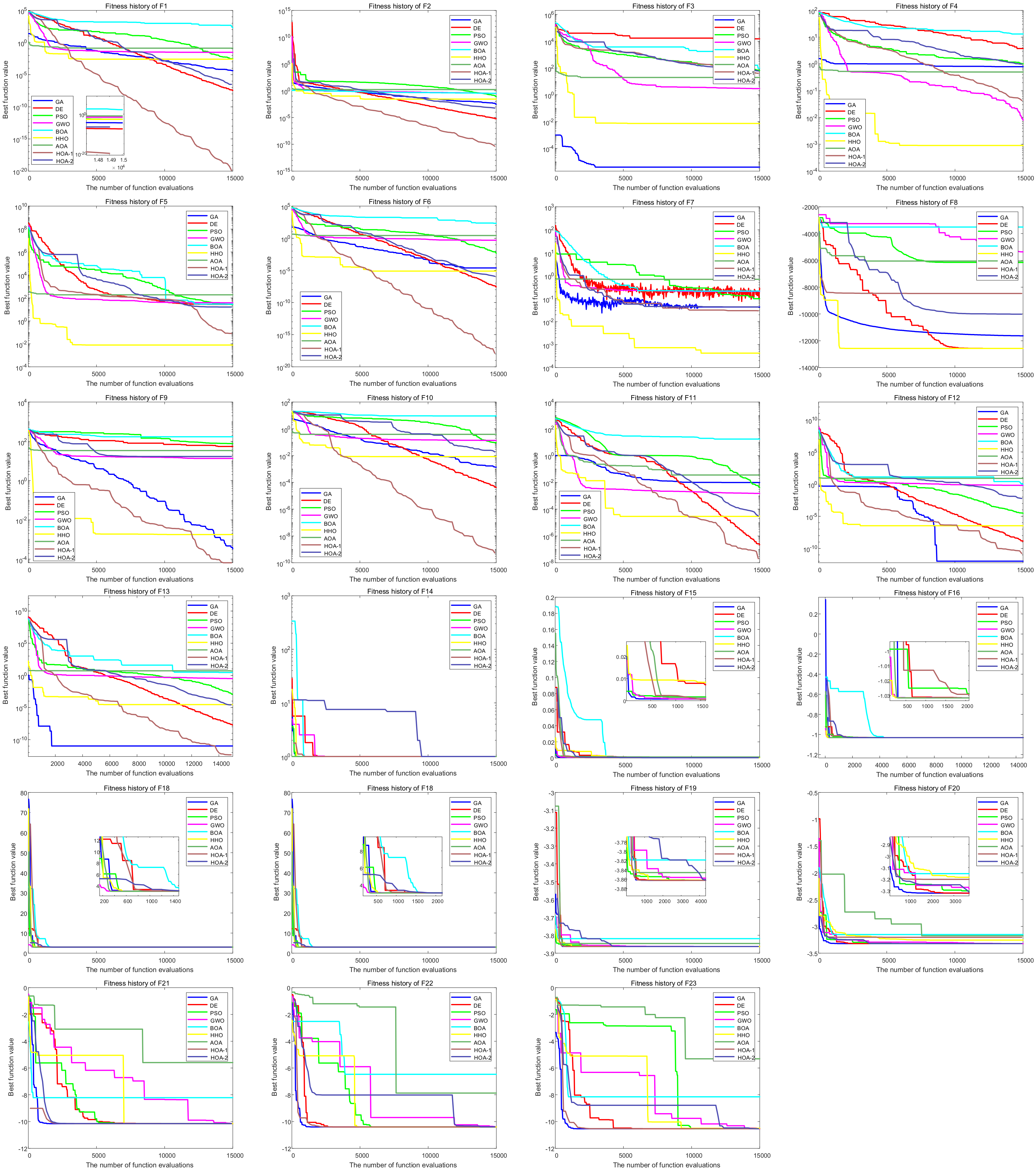
The history of minimum-value searching of benchmark functions is diagrammed in Figure 4. The gentle decrease in the fitness value means the exploitation search was effectively conducted, while the sharp or even vertical decline reflects a better result found by the exploration search. From this point of view, the exploration abilities of GA and HHO are outstanding, and the exploitation ability of HOA-1 is conspicuous. The stepped attenuation of search step length of S-particles attributes more to the descent slope changes in HOA-1 and HOA-2. Note that the number of function evaluations, which is equal to the number of individuals generated in the search space, is used as the coordinate of x-axis. Accordingly, the coordinates of the x-axis of the final minimum values of HOA-1 and HOA-2 are not the same as other compared algorithms, due to the smaller function evaluations number, which is amplified and shown in the subplot of F1 function in Figure 4.
To dissect the search process and convergence of two proposed algorithms, we selected F1, F8 and F14 to represent three types of functions with which to analyze the characteristics of iterative search. The fitness history curves of solving three functions by HOA-1 and HOA-2 are delineated in Figure 5. The fitness history curves show that B-particles in HOA-1 converge faster than those in HOA-2, while B-particles in HOA-2 have better potential for local minima avoidance, which is reflected by the intermittent sharp decline during the iterative search in Figure 5b,c. The initial and final positions of all B-particles of the search in HOA-1 and HOA-2 are displayed in Figure 6 and Figure 7, respectively. Note that the positions of B-particles are represented by the first two coordinates. The B-particles gathered in a subdomain of the search space after the iterative search, which demonstrated that both algorithms possess the ability to drive B-particles to converge and find a high-precision solution.

4.2.2. The Mechanism Explanation by Examples

The core idea of HOF is based on a competition mechanism that tilts computing resources to CBP to make it better, and compels all B-particles to compete for the rewards assigned to the CBP. There is one point to be emphasized: in both HOA-1 and HOA-2, the reward for CBP is granted before the corresponding H1 iteration starts. In other words, once a B-particle takes the title of CBP after one H1 iteration, the reward is conferred on it regardless of whether the alternation of CBP appears in the next iteration. This strategy guarantees the execution of one H2 optimization in every H1 iteration, and is named Normal-Mode, which implies that the number of H2 optimization implementation may not be fixed to 1. There are another two possible situations. One case, called Conservation-Mode, is when H2 optimization is implemented when the ith B-particle becomes CBP and keeps the place until its next personal H1 iteration comes. If other B-particles assume the place of CBP in this period, the ith B-particle will not gain extra assistance from S-particles. The other case is defined as Redundance-Mode, in which H2 optimization is executed as soon as the ith B particle becomes CBP. In this case, there may be more than one H2 optimization in one H1 iteration. These three situations reveal the time delay between the reward of CBP winning and awarding. From the perspective of computational stability, we embed Normal-Mode in HOF to create HOA-1 and HOA-2. By the phenomenon above, this competition mechanism strongly stimulates the competition in B-particles, especially when the numbers of iterations and S-particles in H2 is increased, which exacerbates the imbalance between the CBP and other B-particles.
To make a specific impression on readers, simulated examples were carried out to provide more concrete specification. For better demonstration of the competition mechanism, we used HOA-1 to find the minimum of F8 function and set I b to 150 and I s to 3 in order to weaken the preponderance of CBP. To show the competition for the CBP place among B-particles, we adjusted the parameter T to 10 to preferably exhibit the stepped attenuation of search range.
The situation of CBP alternation is shown in Figure 8, in which Figure 8a gives the alternation of CBP in each H1 iteration and Figure 8b presents the actual execution of H2 optimization in the local region of the red square in Figure 8a. The differences between three situations can be easily observed: in Normal-Mode the H2 optimization is carried out in every H1 iteration, while the number of H2 optimization in Conservation-Mode and in Redundance-Mode decreases five times and increases five times, respectively (the number is 10 in the whole process). Note that in this example, at most, two B-particles become the CBP in one H1 iteration. If the competition is fiercer and more B-particles sequentially become the CBP in one H1 iteration, another example will reflect the result in Figure 9, in which the numbers of H2 optimization carried out in three situations are respectively 16, 14 and 20. In Conservation-Mode, H2 optimization is implemented only when one B-particle remains as CBP for at least two successive H1 iterations. For the performance comparison of different algorithms, Normal-Mode is preferred, due to its fixed amount of computation.
Another typical mechanism is the stepped attenuation of d e l t a S n , which is shown in Figure 10. Because the upper bound and lower bound of each dimension of F8 function is the same, the first element of d e l t a S n is qualified to embody its range variation. All elements of d e l t a S n are reduced to one tenth every 10 H1 iterations. However, it was found in the experiment that the algorithm may not converge to the global optima if the value of T is too small, while a T that is too large causes a loss of solution accuracy in a finite number of iterations. Therefore, further research is warranted to resolve this contradiction.

4.2.3. The Value of Parameter T

In the benchmark functions test, a significant feature of both HOA-1 and HOA-2 is that the parameter T is usually different and tuned according to the test function, which is due to the shrinking mechanism of search space. When the number of iterations in H1 is fixed, decreasing the value of T means to accelerate the process of space shrinking. If this rate is too fast, the minimum search by S-particles will be severely restricted and limited in its ability to help CBP update its position. Only when the optimization in H2 works properly can HOA-1 and HOA-2 seek out a good solution. Conversely, a slow shrinking rate reduces the search efficiency, due to the search space being too large. Meanwhile, a finite iterative number inevitably limits the amount of computation. Hence, in order to promote the smooth progress of optimization, we used different constant values to set the parameter T to control the search precision.
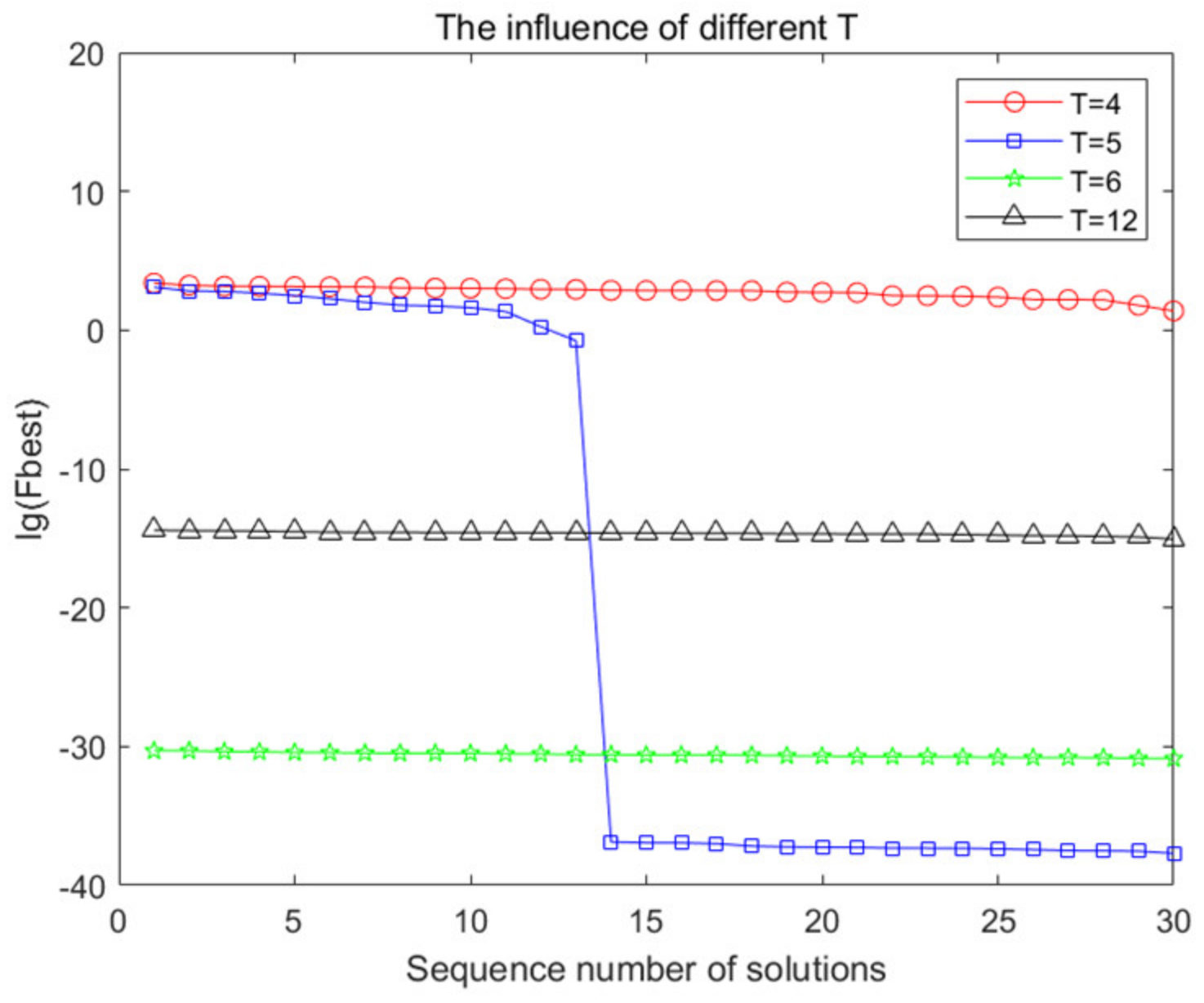
For better elucidation of the influence of different T on a given function, an additional example was provided. Without loss of generality, the F1 function was used to present the phenomenon of performance deterioration and the HOA-1 was assigned to execute the optimization mission. In HOA-1, we added I s from 4 to 10 and set the value of T as 4, 5, 6 and 12. These four group results were collected and compared to show the difference. Each group had 30 solutions, ranked in descending order of F1 function, and all results are displayed in Figure 11, in which Fbest represents the minimum after each run, and the common logarithm of Fbest is taken to conveniently reflect the difference. Three key features can be concluded:
  • A smaller T has the potential to make the algorithm find a better solution.
  • A destabilization of the search may occur when the value of T varies.
  • A T that is too small may impede the algorithm search for the optimal solution.
In this work, the value of T was set by trial and error to achieve a balance between stability and search efficacy, which leaves room for further research to design an adaptive law for parameter adjustment and to mitigate the trouble of manual parameter setting.

5. Applications of the Proposed Methods

In this section, two spacecraft trajectory optimization problems, the multi-impulse minimum fuel orbit transfer and the pursuit-evasion game of two spacecraft, are employed to reflect the capability of the proposed HOA-1 and HOA-2. The former problem is extensively solved by meta-heuristic algorithms [33,44]. The latter problem considers the requirement of tracking a non-cooperative target with maneuvering ability, and has been the subject of much recent attention [45]. The functions of both problems demonstrate strong nonlinearity and variable coupling, even without additional constraints.

5.1. Multi-Impulse Minimum Fuel Orbit Transfer

5.1.1. Problem Formulation and Parameter Setting

Spacecraft orbit optimal transfer by impulsive thrusters is a classical and significant problem. However, an analytic solution of optimal impulsive control for orbit transfer in complicated situations is difficult to obtain when the number of impulses increases and additional complicated constraints are considered. Therefore, a direct approach was developed to construct a general nonlinear programming problem and solve it by advanced optimization algorithms [46]. Relevant research results can be referred to in [44].
Considering the goal of proving the effectiveness of the proposed methods, we chose minimum fuel transfer between two coplanar circular orbits as the problem to be optimized. This has an analytical solution known as the famous Hohmann transfer with two-impulse maneuver. Usually, the fuel consumed is positively correlated with the velocity increment, so the orbit transfer by minimum velocity increment is equivalent to the minimum fuel case. For additional details on the derivation, [47] is recommended. In accordance with the size limit of this paper, a brief introduction of Hohmann transfer is generalized below.
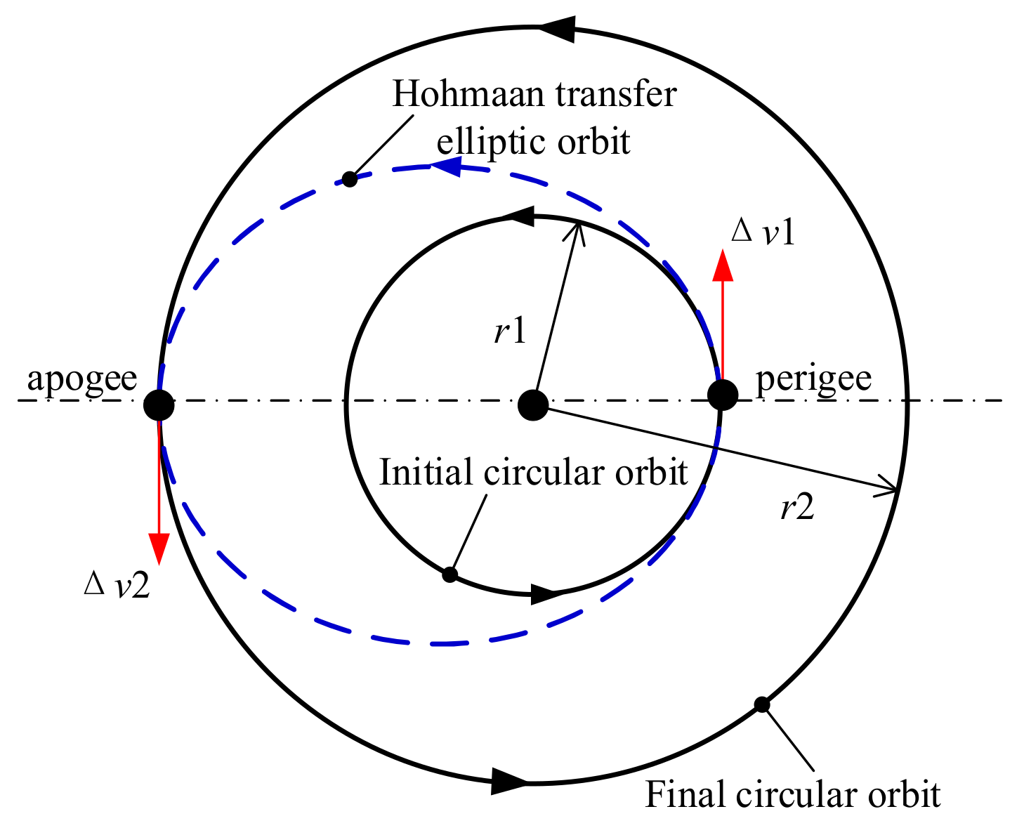
For two coplanar circular orbits around the celestial body, an ellipse connecting two orbits and tangent to them is shown in Figure 12. A spacecraft on the initial orbit can reach the final orbit after two-impulse maneuver Δ v 1 and Δ v 2 . The transfer trajectory is half an ellipse from the perigee to the apogee of the transfer elliptic orbit. Two impulses Δ v 1 and Δ v 2 are given as follows:
Δ v 1 = 2 μ r 2 r 1 ( r 1 + r 2 ) μ r 1 , Δ v 2 = μ r 2 2 μ r 1 r 2 ( r 1 + r 2 )
where μ is the gravitational constant of the celestial body, r1 and r2 are radii of the initial and final circular orbit. According to the characteristic of Hohmann transfer with the theoretical solution of two-impulse maneuver, we designed three cases to test the optimization performance of the proposed two algorithms. As with problem 1 in [44], they concerned two orbits around Mars ( μ = 42,830   k m / s 2 ), with r1 and r2 being 8000 km and 15,000 km, respectively. The three cases are distinguished by search space as listed in Table 6.
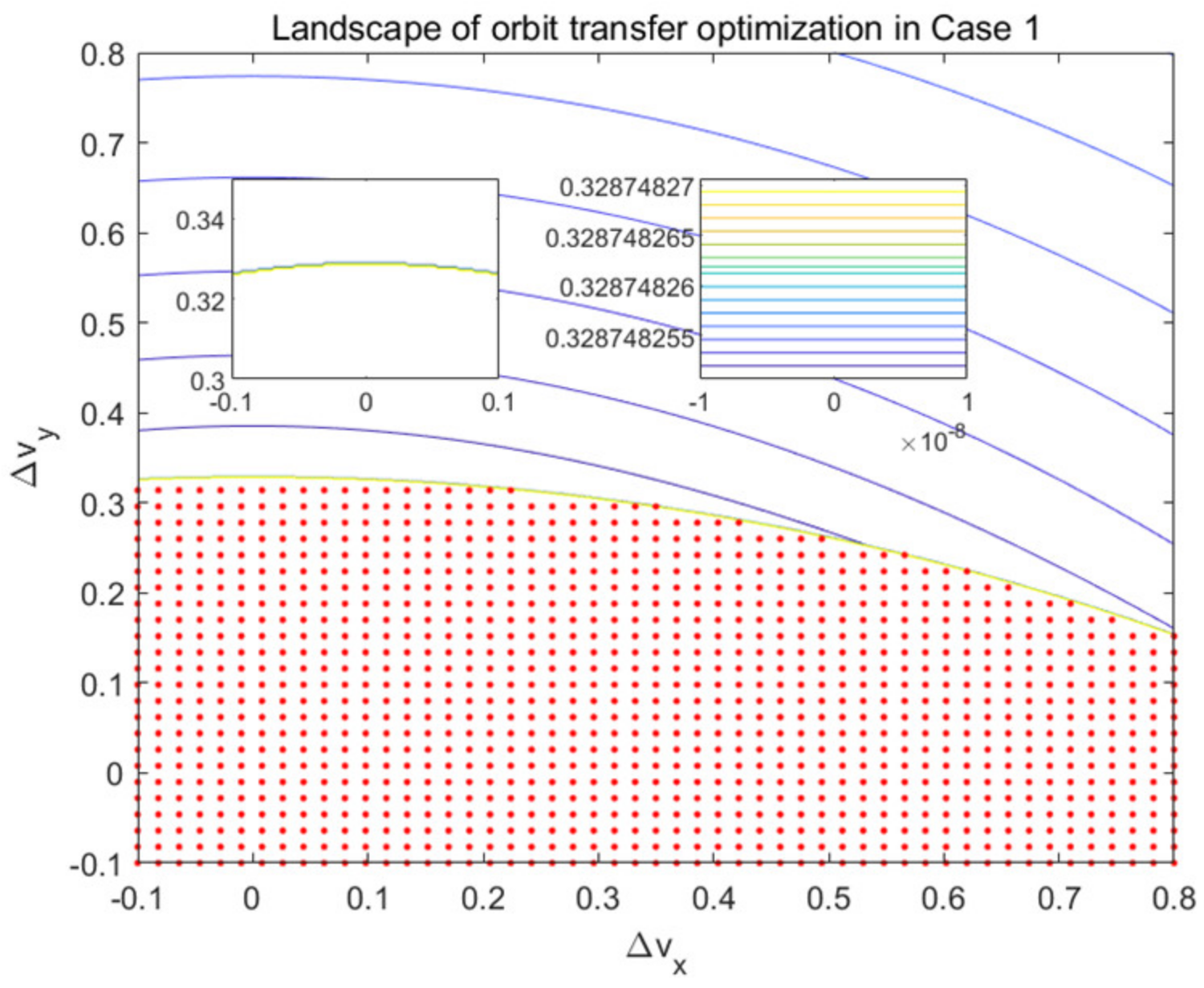
Without loss of generality, the start points of the three cases were all set to the (8000,0). In Case 1, we gave the first in-plane impulse to make the spacecraft leave the initial orbit and applied the second impulse to make it revolve on the final orbit when it reached one point of the final orbit. When the first impulse was provided, the second impulse, if the transfer trajectory intersected the final orbit, was able to be calculated. Therefore, the search space was a 2-dimensional vector whose components were the radial and tangential velocity increments. The landscape is depicted in Figure 13, in which Δ v x and Δ v y represent coordinate components of Δ v 1 , and the domain of the initial velocity impulse that cannot realize orbit transfer is marked with a red dot. Subsequently, we shrank the range of initial velocity increments so as to make the transfer impossible by two-impulse, by which a three-impulse orbit transfer was constructed and the search space became a five-dimensional vector, added to the second 2-dimension impulse and the applied time. Different values of the upper bound of the applied time led to Case 2 and Case 3. In Case 2, the upper bound of applied time allowed the spacecraft to fly one revolution and return to the start point, by which the same total impulse increment with two-impulse Hohmann transfer could be achieved by three-impulse maneuver. However, the upper bound of applied time violated this condition in Case 3, making the result of three-impulse orbit transfer by minimum velocity increment different from Case 2.
DE, GA, PSO, GWO, HHO, AOA, HOA-1 and HOA-2 were used to solve the three cases according to the result of benchmark functions test. The numbers of iterations Imax of all these contrastive algorithms were all set to 400, and the population size was 50. Considering the inconsistency between the dimension of search space and the number of search individuals of these algorithms, we set both I b and I s to 30. The number of S-particles in HOA-1 is equal to N, while that can be changed to 4N in HOA-2 to ensure that the total number of function evaluations is the same as the comparison algorithms. The parameters of DE, GA, PSO, GWO, HHO and AOA were the same as those in Table 1. For more meticulous search, we set α to 0.1 and c to 0 in both HOA-1 and HOA-2.

5.1.2. Results and Discussion

For Case 1 and Case 2, adding in Δ v 1 and Δ v 2 according to Equations (13), the theoretical minimum velocity increment is 0.6091531 km / s 2 . Each algorithm was run 30 times and the best result have been selected and listed in Table 7, in which the best solutions found by these algorithms are bold. The results show that HOA-2 found the best solutions for the three cases, which evidently reflects the superiority of the proposed methods. Because the number of S-particles of HOA-1 should be equal to the problem dimension N, and that of HOA-2 can be properly set to 4N, the amount of computation of HOA-1 is noticeably less than other algorithms, which explains the performance degradation of HOA-1.
The process of orbit transfer using the best solution of three cases is diagrammed in Figure 14, which is consistent with the previous analysis and proves the correctness of the results. Comparing the results of Case 1 and Case 2, it can be observed that the difficulty of finding the optimal solution increases when the dimensions of the search space increase. In a similar way, further reduction in velocity range can construct the orbit transfer by more impulses and increase the difficulty of spacecraft orbit maneuver optimization. Nevertheless, uncertain spacecraft trajectory is more likely with the increasing number of impulses [48].

5.2. Pursuit-Evasion Game of Two Spacecraft

5.2.1. Problem Formulation and Parameters Setting

Spacecraft pursuit-evasion is a typical game problem, in which the pursuing spacecraft attempts to capture the target while the evading spacecraft strives for escape. Accordingly, this pursuit-evasion problem is a zero-sum differential game. As a result of the great difficulty of an analytical solution derivation, the numerical methods have been extensively used in recent decades. The indirect method of solving this problem is to derive the necessary optimal conditions, transform it into a two-point boundary value problem (TPBVP) and find a saddle point by numerical methods. In this paper, the TPBVP solution is used to test the performance of the proposed methods. The dynamic model and necessary conditions derivation are adopted from [49], and a transcription is provided below.
The differential equations of the pursuit-evasion game are written as follows:
X ˙ = A ( t ) X + T P U P + T E U E
where X = [ x P , y P , z P , x ˙ P , y ˙ P , z ˙ P , x E , y E , z E , x ˙ E , y ˙ E , z ˙ E ] T is the state variable of positions and velocities of two spacecraft in the LVLH coordinate system of a virtual spacecraft in circular reference orbit, and the subscripts P and E represent the pursuing spacecraft and the evading spacecraft, respectively. U P = [ 0 1 × 3 , u P x , u P y , u P z , 0 1 × 6 ] T and U E = [ 0 1 × 9 , u E x , u E y , u E z ] T represent the direction vector of control exerted on two spacecraft, and satisfy the restraint conditions u I x 2 + u I y 2 + u I z 2 1 , in which I means P or E. T P and T E are the value of maximum thrust per unit mass of two spacecraft. Clohessy–Wiltshire equations [50] are used to describe the relative motion of two spacecraft with respect to the reference rotating coordinate system, and the matrix A ( t ) can be expressed by Equation (15).
A ( t ) = A P ( t ) 0 0 A E ( t ) , A P ( t ) = A E ( t ) = 0 0 0 1 0 0 0 0 0 0 1 0 0 0 0 0 0 1 3 ω 2 0 0 0 2 ω 0 0 0 0 2 ω 0 0 0 0 ω 2 0 0 0
where ω is the constant rotational angular velocity of reference coordinate system in the gravitational field of the Earth. Set the terminal time as tf, so the payoff function is as follows:
J = 1 2 [ ( x P x E ) 2 + ( y P y E ) 2 + ( z P z E ) 2 ] t = t f
Therefore, the spacecraft pursuit-evasion game can be described thus: the goal of pursuing spacecraft is to change U P to minimize J , while the evading spacecraft aims at maximum by J by U E .
The adjoint variable λ = [ λ P , λ E ] T is introduced corresponding to X, in which λ I = [ λ I x , λ I y , λ I z , λ I x ˙ , λ I y ˙ , λ I z ˙ ] T and I = P , E . Construct the Hamiltonian function as H = λ T X , and the control of two spacecraft can be derived according to the minimum principle and Cauchy–Schwarz inequality.
u P x = λ P x λ P x 2 + λ P y 2 + λ P z 2 u P y = λ P y λ P x 2 + λ P y 2 + λ P z 2 u P z = λ P z λ P x 2 + λ P y 2 + λ P z 2 , u E x = λ E x λ E x 2 + λ E y 2 + λ E z 2 u E y = λ E y λ E x 2 + λ E y 2 + λ E z 2 u E z = λ E z λ E x 2 + λ E y 2 + λ E z 2
The adjoint variable λ = [ λ P , λ E ] T satisfies the differential equations in (18).
λ ˙ = H X T
The transversal condition is derived by (19).
λ ( t f ) = J X ( t f ) T = [ λ P x , λ P y , λ P z , 0 1 × 3 , λ E x , λ E y , λ E z , 0 1 × 3 ] t = t f T
So far, the TPBVP has been derived completely. Input the guess of initial adjoint variables to the optimization algorithms and minimize J to test the performance of the proposed methods. Relevant parameters are set as follows:
ω = μ / r 0 3 , r 0 = 6900   km , μ = 3.986   ×   10 5   km 3 / s 2 t f = 1500   s T P = 0.02   g , T E = 0.01   g ,     g = 0.0098   km / s 2 X ( 0 ) = [ X P ( 0 ) , X E ( 0 ) ] T X P ( 0 ) = [ 0 , 5.12 , 6.21 , 0.0268 , 4.715 × 10 5 , 0.0011 ] X E ( 0 ) = [ 9.92 , 24.12 , 0 , 0.2678 , 0.005608 , 0 ]  
A reasonable initial value of adjoint variable λ 0 is given in (21), and the corresponding J is 0.489126783247148.
λ 0 = [ λ 1 , λ 2 , , λ 11 , λ 12 ] T λ 1 = 1.828416833471 × 10 3 , λ 2 = 1.087432620919 × 10 3 λ 3 = 1.0996952525 × 10 5 , λ 4 = 1.31744718559753 λ 5 = 0.092072105520415 , λ 6 = 9.50453008156 × 10 3 λ 7 = 2.96673065336 × 10 4 , λ 8 = 1.01857391376 × 10 4 λ 9 = 1.4412237482 × 10 5 , λ 10 = 0.408955063275592 λ 11 = 5.43535547235 × 10 3 , λ 12 = 8.00595379572 × 10 4
According to λ 0 , two cases were designed, as displayed in Table 8, to test the performance of the same eight algorithms as in Section 5.1. Note that in Table 8, [1]12 is a 12-dimension column vector with all elements being 1. The parameters of these algorithms are almost the same as in Section 5.1, except that we changed I b to 40 for HOA-1 to improve its performance, and the number of S-particles of HOA-1 and HOA-2 were respectively set to 12 and 20, to ensure a smaller amount of computation compared with other algorithms.

5.2.2. Results and Discussion

For both cases, each algorithm was run 10 times and the best result was selected and listed in Table 9, in which the best solutions are bold. The results show that HOA-2 performed best in this test, while the performance of HOA-1 is poorer than GWO and HOA-2, but better than other algorithms. Considering the difference between the two cases, it can be concluded that Case 1 examined the exploration of algorithms, while exploitation was more important in Case 2. Thus, the result is consistent with the previous statement that hierarchical optimization is designed to assign more computation resources to the CBP position update.
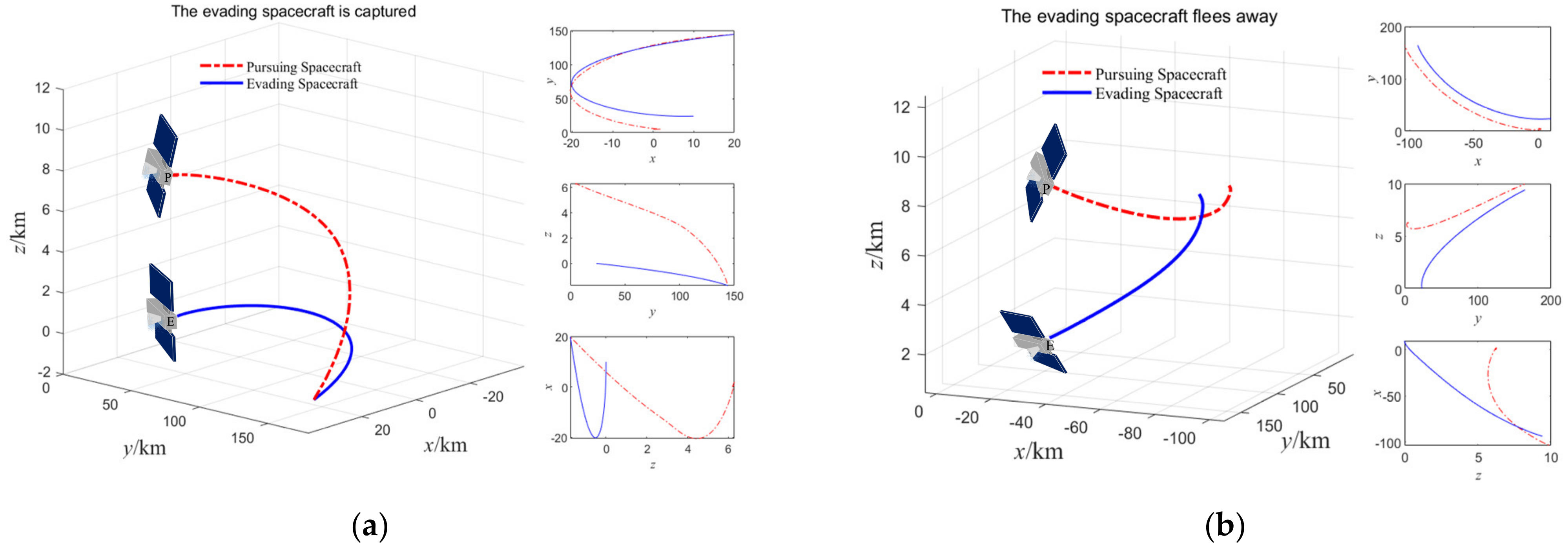
It is universally accepted that the solution of TPBVP is difficult to acquire due to the strongly sensitive characteristic of the initial guess value of the adjoint variable that lacks physical meaning. However, a better initial guess may help us solve the TPBVP by the multiple shooting method, whose limitation lies in the high requirement of initial value. To illustrate the diversion caused by poorer initial adjoint variables, an example is provided in which two initial values of adjoint variable are used as input to the multiple shooting method to check whether the evading spacecraft could be captured by the designed control (17). The first initial value is λ 0 , and the second one λ 0 is obtained by decreasing the first element of λ 0 by 20%. The payoff function J with λ 0 is 36.448. The result is diagrammed in Figure 15, which shows that a tiny change in the initial value of TPBVP had a great impact on the result. Therefore, the proposed methods can effectively help to guess the initial value of TPBVP.
In these two spacecraft trajectory optimization problems, HOA-2 performed better than HOA-1. This can be explained by two factors. The first is that the function evaluation number of HOA-1 is significantly less than other algorithms. The second factor is that the S-particle multidimensional sampling, based on the Gaussian distribution function in HOA-2, performs more efficiently when I s increases. Therefore, the proper allocation of the numbers of B-particles and S-particles can make better use of hierarchical optimization algorithms. We suggest that HOA-1 is suitable when the problem dimension is relatively large, and otherwise HOA-2 is preferred, especially when the S-particles can be set to a much larger number than the problem dimension.

6. Conclusions

For improving the search ability of the best individual compared with others, a hierarchical optimization frame is proposed, in which B-particles synergistically explore the search space, and a local search performed by S-particles is conducted to update the position of the best B-particle. Based on this framework, two algorithms (HOA-1 and HOA-2) were designed. The local search in HOA-1 is a type of pattern search with random factors, and that of HOA-2 is based on the sampling in the iteratively updated Gaussian distributions. Considering the limitations of regular benchmark functions, twenty-three variant benchmark functions were designed and solved to accurately reflect the performance of the proposed algorithms and compared algorithms. The experiment results show that HOA-1 outperforms other algorithms in the benchmark function test. In order to further verify the feasibility and superiority of the proposed algorithms, two spacecraft trajectory optimization problems, multiple-impulse orbit transfer and spacecraft pursuit-evasion game, were introduced, due to their complexity and challenges. The HOA-2 algorithm excels outstandingly in solving trajectory optimization problems. In HOA-1, the number of S-particles should be identical to the dimension of the problem, which partially limits its performance and adaptivity.
The parameter T greatly influences the performance of proposed algorithms, especially on the convergence speed. Generally, a larger T is suitable to solve the unimodal function, while a smaller T is preferred in solving the multimodal function. Also, the allocation of function evaluation numbers between the B-particles and S-particles is important to determine the search efficiency. For future research, searching strategy design and techniques of parameter setting are both promising research directions for promoting the development of hierarchical optimization.

Author Contributions

Conceptualization, H.H. and P.S.; methodology, H.H. and P.S.; software, H.H.; investigation, H.H.; writing—original draft preparation, H.H.; writing—review and editing, P.S and Y.Z.; funding acquisition, P.S. All authors have read and agreed to the published version of the manuscript.

Funding

This work is supported by the National Natural Science Foundation of China (No. 11572019).

Conflicts of Interest

The authors declare no conflict of interest.

Appendix A. Benchmark Functions

Table A1. Unimodal benchmark functions.
FunctionDimRangefmin
F 1 = i = 1 Dim x i 2 30[−100, 100]0
F 2 = i = 1 Dim x i + i = 1 Dim x i 30[−10, 10]0
F 3 = i = 1 Dim j = 1 i x j 2 30[−100, 100]0
F 4 = x i , 1 i Dim 30[−100, 100]0
F 5 = i = 1 Dim 100 ( x i + 1 x i 2 ) 2 + ( x i + 1 ) 2 30[−30, 30]0
F 6 = i = 1 Dim ( x i + 0.5 ) 2 30[−100, 100]0
F 7 = i = 1 Dim i x i 4 + r a n d o m [ 0 , 1 ) 30[−1.28, 1.28]0
Table A2. Multimodal benchmark functions.
FunctionDimRangefmin
F 8 = i = 1 Dim x i sin ( x i ) 30[−500, 500] 419 × Dim
F 9 = i = 1 Dim x i 2 10 cos ( 2 π x i ) + 10 30[−5.12, 5.12]0
F 10 = 20 exp 0.2 i = 1 Dim x i 2 / Dim exp i = 1 Dim cos ( 2 π x i ) / Dim + 20 + e 30[−32, 32]0
F 11 = i = 1 Dim x i 2 / 4000 i = 1 Dim cos x i / i + 1 30[−600, 600]0
F 12 = π Dim sin ( π y 1 ) + i = 1 Dim 1 ( y i 1 ) 2 [ 1 + 10 sin 2 ( π y i + 1 ) ] + ( y Dim 1 ) 2 + 1 Dim u ( x i , 10 , 100 , 4 ) y i = 1 + x i + 1 4 , u ( x i , a , k , m ) = k ( x i a ) m x i > a 0 a < x i < a k ( x i a ) m x i < a 30[−50, 50]0
F 13 = 0.1 sin 2 ( 3 π x 1 ) + i = 1 Dim 1 ( x i 1 ) 2 [ 1 + sin 2 ( 3 π x i + 1 ) ] + ( x Dim 1 ) 2 [ 1 + sin 2 ( 2 π x Dim ) ] + 1 Dim u ( x i , 5 , 100 , 4 ) 30[−50, 50]0
Table A3. Fixed-dimension benchmark functions.
FunctionDimRangefmin
F 14 = 1 500 + j = 1 25 1 j + i = 1 2 ( x i a i j ) 6 1 2[−65, 65]0.998
F 15 = i = 1 11 a i x 1 ( b i 2 + b i x 2 ) b i 2 + b i x 3 + x 4 2 4[−5, 5]0.0003
F 16 = 4 x 1 2 2.1 x 1 4 + 1 3 x 1 6 + x 1 x 2 4 x 2 2 + 4 x 2 4 2[−5, 5]−1.0316
F 17 = x 2 5.1 4 π 2 x 1 2 + 5 π x 1 6 2 + 10 1 1 8 π cos x 1 + 10 2[−5, 5]0.398
F 18 = 1 + x 1 + x 2 + 1 2 19 14 x 1 + 3 x 1 2 14 x 2 + 6 x 1 x 2 + 3 x 2 2 × 30 + 2 x 1 3 x 2 2 18 32 x 1 + 12 x 1 2 + 48 x 2 36 x 1 x 2 + 27 x 2 2 2[−2, 2]3
F 19 = i = 1 4 c i exp j = 1 3 a i j x j p i j 2 3[0, 1]−3.86
F 20 = i = 1 4 c i exp j = 1 6 a i j x j p i j 2 6[0, 1]−3.32
F 21 = i = 1 5 X a i T X a i + c i 1 4[0, 10]−10.1532
F 22 = i = 1 7 X a i T X a i + c i 1 4[0, 10]−10.4028
F 23 = i = 1 10 X a i T X a i + c i 1 4[0, 10]−10.5363

References

  1. Zhang, P.; Xu, Z.; Wang, Q.; Fan, S.; Cheng, W.; Wang, H.; Wu, Y. A novel variable selection method based on combined moving window and intelligent optimization algorithm for variable selection in chemical modeling. Spectrochim. Acta Part A Mol. Biomol. Spectrosc. 2021, 246, 118986. [Google Scholar] [CrossRef]
  2. Lin, C.; Wang, J.; Lee, C. Pattern recognition using neural-fuzzy networks based on improved particle swam optimization. Expert Syst. Appl. 2009, 36, 5402–5410. [Google Scholar] [CrossRef]
  3. Majeed, A.; Hwang, S. A Multi-Objective Coverage Path Planning Algorithm for UAVs to Cover Spatially Distributed Regions in Urban Environments. Aerospace 2021, 8, 343. [Google Scholar] [CrossRef]
  4. Gao, X.Z.; Nalluri, M.S.R.; Kannan, K.; Sinharoy, D. Multi-objective optimization of feature selection using hybrid cat swarm optimization. Sci. China Technol. Sci. 2021, 64, 508–520. [Google Scholar] [CrossRef]
  5. Singh, T. A novel data clustering approach based on whale optimization algorithm. Expert Syst. 2021, 38, e12657. [Google Scholar] [CrossRef]
  6. Pontani, M.; Ghosh, P.; Conway, B. Particle swarm optimization of multiple-burn rendezvous trajectories. J. Guid. Control Dyn. 2012, 35, 1192–1207. [Google Scholar] [CrossRef]
  7. Wagner, S.; Wie, B. Hybrid algorithm for multiple gravity-assist and impulsive delta-V maneuvers. J. Guid. Control Dyn. 2015, 38, 2096–2107. [Google Scholar] [CrossRef] [Green Version]
  8. Wang, X.; Zhang, H.; Bai, S.; Yue, Y. Design of agile satellite constellation based on hybrid-resampling particle swarm optimization method. Acta Astronaut. 2021, 178, 595–605. [Google Scholar] [CrossRef]
  9. Wu, C.; Xu, R.; Zhu, S.; Cui, P. Time-optimal spacecraft attitude maneuver path planning under boundary and pointing constraints. Acta Astronaut. 2017, 137, 128–137. [Google Scholar] [CrossRef]
  10. Mirjalili, S.; Mirjalili, S.M.; Lewis, A. Grey wolf optimizer. Adv. Eng. Softw. 2014, 69, 46–61. [Google Scholar] [CrossRef] [Green Version]
  11. Holland, J.H. Genetic algorithms. Sci. Am. 1992, 267, 66–72. [Google Scholar] [CrossRef]
  12. Yao, X.; Liu, Y.; Lin, G. Evolutionary programming made faster. IEEE Trans. Evol. Comput. 1999, 3, 82–102. [Google Scholar] [CrossRef] [Green Version]
  13. Storn, R.; Price, K. Differential evolution—A simple and efficient heuristic for global optimization over continuous spaces. J. Glob. Optim. 1997, 11, 341–359. [Google Scholar] [CrossRef]
  14. Juang, C. A hybrid of genetic algorithm and particle swarm optimization for recurrent network design. IEEE Trans. Syst. Man. Cybern. 2004, 34, 997–1006. [Google Scholar] [CrossRef] [PubMed]
  15. Zhu, X.; Zhang, H.; Gao, Y. Correlations between the scaling factor and fitness values in differential evolution. IEEE Access. 2020, 8, 32100–32120. [Google Scholar] [CrossRef]
  16. Smith, J. Coevolving memetic algorithms: A review and progress report. IEEE Trans. Syst. Man Cybern. Part B-Cybern. 2007, 37, 6–17. [Google Scholar] [CrossRef] [PubMed] [Green Version]
  17. Smith, J.; Fogarty, T. Operator and parameter adaptation in genetic algorithms. Soft Comput. 1997, 1, 81–87. [Google Scholar] [CrossRef] [Green Version]
  18. Kennedy, J.; Eberhart, R. Particle swarm optimization. In Proceedings of the 1995 IEEE International Conference on Neural Networks, Perth, WA, USA, 27 November–1 December 1995; pp. 1942–1948. [Google Scholar] [CrossRef]
  19. Shi, Y.; Eberhart, R. A modified particle swarm optimizer. In Proceedings of the 1998 IEEE Word Congress on Computational Intelligence, Anchorage, AK, USA, 4–9 May 1998; pp. 69–73. [Google Scholar] [CrossRef]
  20. Kennedy, J.; Eberhart, R. A discrete binary version of the particle swarm algorithm. In Proceedings of the 1997 IEEE International Conference on Systems, Man, and Cybernetics-Computational Cybernetics and Simulation, Orlando, FL, USA, 12–15 October 1997; pp. 4104–4108. [Google Scholar] [CrossRef]
  21. Rana, S.; Jasola, S.; Kumar, R. A review on particle swarm optimization algorithms and their applications to data clustering. Artif. Intell. Rev. 2011, 35, 211–222. [Google Scholar] [CrossRef]
  22. Yang, X. Firefly algorithm, stochastic test functions and design optimization. Int. J. Bio-Inspired Comput. 2010, 2, 78–84. [Google Scholar] [CrossRef]
  23. Heidari, A.A.; Mirjalili, S.; Faris, H.; Aljarah, I.; Mafarja, M.; Chen, H. Harris hawks optimization: Algorithm and applications. Future Gener. Comput. Syst. 2019, 97, 849–872. [Google Scholar] [CrossRef]
  24. Gao, K.; Cao, Z.; Zhang, L.; Han, Y.; Pan, Q. A review on swarm intelligence and evolutionary algorithms for solving flexible job shop scheduling problems. IEEE-CAA J. Autom. Sin. 2019, 6, 904–916. [Google Scholar] [CrossRef]
  25. Kirkpatrick, S.; Gelatt, C.D.; Vecchi, M.P. Optimization by simulated annealing. Science 1983, 220, 671–680. [Google Scholar] [CrossRef] [PubMed]
  26. Rashedi, E.; Nezamabadi-Pour, H.; Saryazdi, S. GSA: A gravitational search algorithm. Inf. Sci. 2009, 179, 2232–2248. [Google Scholar] [CrossRef]
  27. Mirjalili, S. SCA: A Sine Cosine Algorithm for solving optimization problems. Knowl.-Based Syst. 2016, 96, 120–133. [Google Scholar] [CrossRef]
  28. Abualigah, L.; Diabat, A.; Mirjalili, S.; Elaziz, M.A.; Gandomi, A.H. The arithmetic optimization algorithm. Comput. Methods Appl. Mech. Engrgy 2021, 376, 113609. [Google Scholar] [CrossRef]
  29. Wolpert, D.; Macready, W.G. No free lunch theorems for optimization. IEEE Trans. Evolut. Comput. 1997, 1, 67–82. [Google Scholar] [CrossRef] [Green Version]
  30. Passino, K. Biomimicry of bacterial foraging for distributed optimization and control. IEEE Control Syst. Mag. 2002, 22, 52–67. [Google Scholar] [CrossRef]
  31. Jin, M.; Lu, H. A multi-subgroup hierarchical hybrid of genetic algorithm and particle swarm optimization. Control Theory Appl. 2013, 30, 1231–1238. [Google Scholar] [CrossRef]
  32. Liu, L.; Guo, Y. Multi-objective optimization for attitude maneuver of liquid-filled flexible spacecraft based on improved hierarchical optimization algorithm. Appl. Soft Comput. 2020, 96, 106598. [Google Scholar] [CrossRef]
  33. Vasile, M.; Locatelli, M. A hybrid multiagent approach for global trajectory optimization. J. Glob. Optim. 2009, 44, 461–479. [Google Scholar] [CrossRef] [Green Version]
  34. Zuiani, F.; Vasile, M. Multi Agent Collaborative Search based on Tchebycheff decomposition. Comput. Optim. Appl. 2013, 56, 189–208. [Google Scholar] [CrossRef] [Green Version]
  35. Arab, A.; Alfi, A. An adaptive gradient descent-based local search in memetic algorithm applied to optimal controller design. Inf. Sci. 2015, 299, 117–142. [Google Scholar] [CrossRef]
  36. Bao, Y.; Hu, Z.; Xiong, T. A PSO and pattern search based memetic algorithm for SVMs parameters optimization. Neurocomputing 2013, 117, 98–106. [Google Scholar] [CrossRef] [Green Version]
  37. Lin, S. A parallel processing multi-coordinate descent method with line search for a class of large-scale optimization-algorithm and convergence. In Proceedings of the 30th IEEE Conference on Decision and Control, Brighton, UK, 11–13 December 1991. [Google Scholar] [CrossRef]
  38. Kennedy, J. Bare bones particle swarms. In Proceedings of the 2003 IEEE Swarm Intelligence Symposium, Indianapolis, IN, USA, 26 April 2003; pp. 80–87. [Google Scholar] [CrossRef]
  39. Zhang, E.; Wu, Y.; Chen, Q. A practical approach for solving multi-objective reliability redundancy allocation problems using extended bare-bones particle swarm optimization. Reliab. Eng. Syst. Saf. 2014, 127, 65–76. [Google Scholar] [CrossRef]
  40. Zhang, Y.; Gong, D.; Ding, Z. A bare-bones multi-objective particle swarm optimization algorithm for environmental/economic dispatch. Inf. Sci. 2012, 192, 213–227. [Google Scholar] [CrossRef]
  41. Hansen, N.; Muller, S.; Koumoutsakos, P. Reducing the time complexity of the derandomized evolution strategy with covariance matrix adaptation (CMA-ES). Evol. Comput. 2003, 11, 1–18. [Google Scholar] [CrossRef]
  42. Arora, S.; Singh, S. Butterfly optimization algorithm: A novel approach for global optimization. Soft Comput. 2019, 23, 715–734. [Google Scholar] [CrossRef]
  43. Derrac, J.; García, S.; Molina, D.; Herrera, F. A practical tutorial on the use of nonparametric statistical tests as a methodology for comparing evolutionary and swarm intelligence algorithms. Swarm Evol. Comput. 2011, 1, 3–18. [Google Scholar] [CrossRef]
  44. Abdelkhalik, O.; Mortari, D. N-impulse orbit transfer using genetic algorithms. J. Spacecr. Rockets 2007, 44, 456–460. [Google Scholar] [CrossRef]
  45. Wang, X.; Shi, P.; Zhao, Y.; Sun, Y. A pre-trained fuzzy reinforcement learning method for the pursuing satellite in a one-to-one game in space. Sensors 2020, 20, 2253. [Google Scholar] [CrossRef]
  46. Hughes, S.; Mailhe, L.; Guzman, J. A comparison of trajectory optimization methods for the impulsive minimum fuel rendezvous problem. Adv. Astronaut. Sci. 2003, 113, 85–104. [Google Scholar]
  47. Curtis, H. Orbital Mechanics for Engineering Students; Elsevier Butterworth-Heinemann: Oxford, UK, 2010; pp. 257–264. [Google Scholar] [CrossRef]
  48. Yang, Z.; Luo, Y.; Zhang, J. Nonlinear semi-analytical uncertainty propagation of trajectory under impulsive maneuvers. Astrodynamics 2019, 3, 61–77. [Google Scholar] [CrossRef]
  49. Sun, S.; Zhang, Q.; Loxton, R.; Li, B. Numerical solution of a pursuit-evasion differential game involving two spacecraft in low Earth orbit. J. Ind. Manag. Optim. 2015, 11, 1127–1147. [Google Scholar] [CrossRef]
  50. Clohessy, W.; Wiltshire, R. Terminal guidance system for satellite rendezvous. J. Aerosp. Sci. 1960, 11, 653–658. [Google Scholar] [CrossRef]
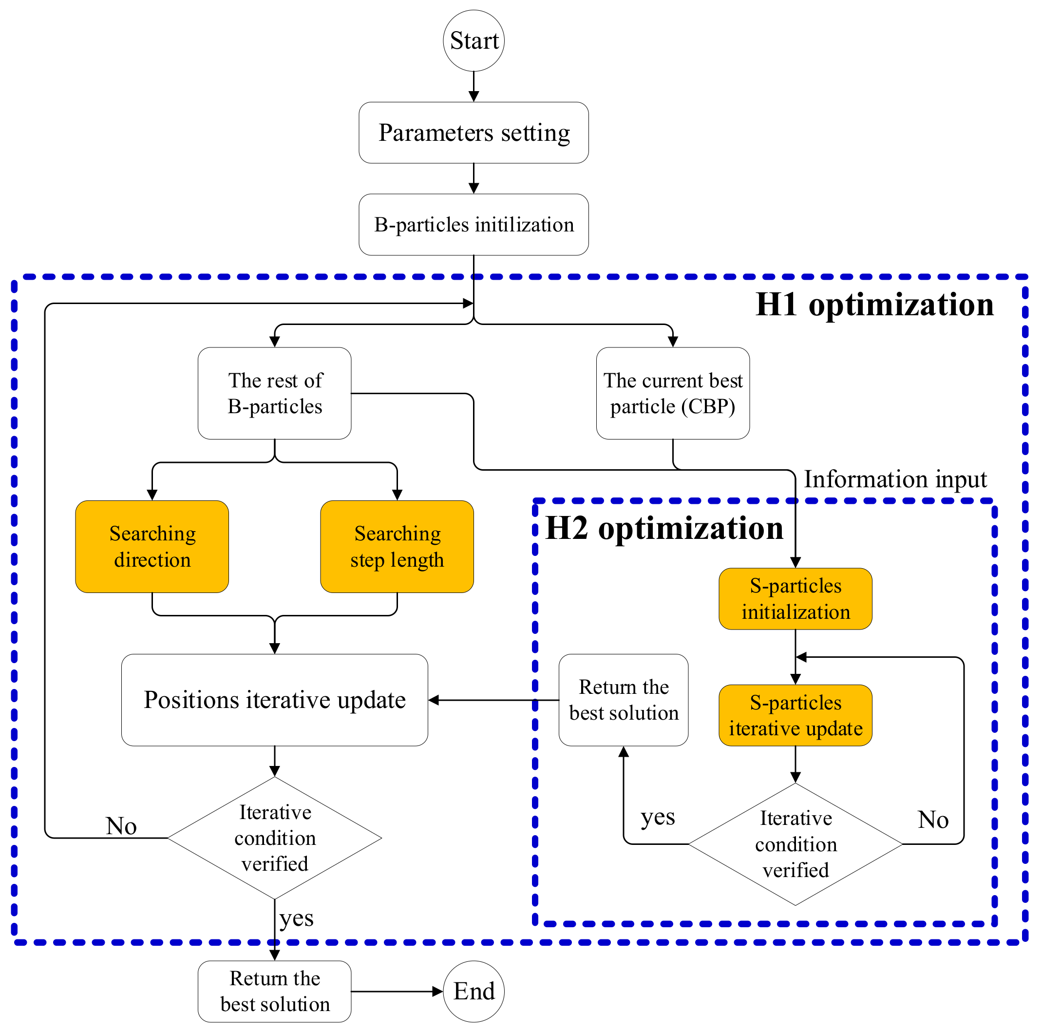
Figure 1. Flowchart of HOF.
Aerospace 09 00081 g001
Figure 2. Update process of CBP in HOF.
Aerospace 09 00081 g002aAerospace 09 00081 g002b
Figure 3. The difference between two specifications of μ and σ .
Aerospace 09 00081 g003
Figure 4. Searching history of benchmark functions.
Aerospace 09 00081 g004
Figure 5. The history fitness curves solved by HOA-1 and HOA-2 for (a) F1; (b) F8; (c) F14.
Aerospace 09 00081 g005
Figure 6. Initial and final positions of B-particles solved by HOA-1 for (a) F1; (b) F8; (c) F14.
Aerospace 09 00081 g006
Figure 7. Initial and final positions of B-particles solved by HOA-2 for (a) F1; (b) F8; (c) F14.
Aerospace 09 00081 g007
Figure 8. Alternation of L1 and the comparison of three modes (a) sequence number of the best B-particle in H1 iteration; (b) Local diagram of the sequence number of B-particle with H2 optimization in three modes.
Aerospace 09 00081 g008
Figure 9. Complicated example for three modes comparison.
Aerospace 09 00081 g009
Figure 10. Stepped decrease of d e l t a S n .
Aerospace 09 00081 g010
Figure 11. The influence of different values of T on optimized results.
Aerospace 09 00081 g011
Figure 12. Diagram of Hohmann transfer.
Aerospace 09 00081 g012
Figure 13. The landscape of orbit transfer in Case 1.
Aerospace 09 00081 g013
Figure 14. The orbit transfer of (a) Case 1; (b) Case 2; (c) Case 3.
Aerospace 09 00081 g014
Figure 15. The result based on two sets of initial values of adjoint variables (a) the result with λ 0 as input; (b) the result with λ 0 as input.
Aerospace 09 00081 g015
Table 1. Parameters setting.
AlgorithmParameters
GAPc = 0.8, Pm = 0.2, Pr = 1.5
DEF = 0.3, CR = 0.2
PSOωmax = 0.9, ωmin = 0.4, c1 = c2 = 2
GWOa = 2(1-i/Imax), i is the current iteration
BOAa = 0.1 + 0.2 × i/Imax, i is the current iteration, c = 0.01, p = 0.8
HHOβ = 1.5, J = 2(1-r5), r5~U(0,1)
AOA α = 5, μ = 0.5
HOA-1 α = 0.3, c1 = 1, c2 = 0.3, c = 1
HOA-2 α = 0.3, c1 = 1, c2 = 0.3, c = 1
Table 2. Results of unimodal benchmark functions.
F HOA-1HOA-2GADEPSOGWOBOAHHOAOA
F1B3.28 × 10−16T = 63.16 × 10⁻⁷T = 156.73 × 10−91.12 × 10−81.13 × 10−31.88 × 10−668.02.43 × 10−60.134
A8.87 × 10−169.34 × 10−61.33 × 10−81.13 × 10−20.01573.18 × 10−24070.01060.172
S3.28 × 10−168.63 × 10−63.78 × 10−90.05420.01270.01531550.02410.0157
F2B4.38 × 10−10T = 81.05 × 10⁻⁴T = 151.92 × 10−44.92 × 10−60.05680.1740.2259.46 × 10−31.65
A0.2375.21 × 10−43.74 × 10−48.67 × 10−60.1750.4172.390.04891.81
S1.106.26 × 10−39.17 × 10−52.57 × 10−60.8190.1371.670.03680.0763
F3B75.7T = 4035.2T = 301.14 × 10−181.54 × 10440.82.2772.93.62 × 10−414.1
A3141897.04 × 10−111.88 × 10499.76.934970.14273.1
S14689.52.75 × 10−102.64 × 10335.92.743250.231107
F4B0.0302T = 350.664T = 300.8043.590.9315.38 × 10−312.21.52 × 10−50.500
A0.1362.391.766.261.350.27416.04.94 × 10−30.504
S0.1911.240.5473.150.2400.2121.333.78 × 10−36.63 × 10⁻³
F5B0.173T = 4014.7T = 30N/A21.833.33629.05.76 × 10−4183
A52.641.1N/A11219064.129.10.0186223
S33.223.8N/A81.822314.60.1580.025615.0
F6B1.36 × 10−18T = 103.35 × 10⁻⁷T = 151.55 × 10−55.82 × 10−93.59 × 10−35.80 × 10−51403.37 × 10−82.57
A2.82 × 10−183.51 × 10−54.93 × 10−56.82 × 10−40.02010.7184659.17 × 10−53.20
S1.03 × 10−185.63 × 10−53.46 × 10−53.67 × 10−30.02170.3651621.29 × 10−40.286
F7B0.0135T = 700.0329T = 250.03030.08180.1680.09230.2045.99 × 10−50.684
A0.04800.07470.09160.1980.3770.1910.2999.79 × 10−40.724
S0.01920.02280.03640.05720.1470.05000.06911.11 × 10−30.0133
Table 3. Results of multimodal benchmark functions.
F HOA-1HOA-2GADEPSOGWOBOAHHOAOA
F8B−9.19 × 10³T = 40−10.0 × 10⁴T = 25−1.21 × 10⁴−1.26 × 10⁴−8.23 × 10³−7.51 × 10³−3.53 × 10³−1.26 × 10⁴−6.21 × 10³
A−7.40 × 10³−7.83 × 10³−1.13 × 10⁴−1.24 × 10⁴−5.56 × 10³−5.95 × 10³−2.67 × 10³−1.26 × 10⁴−5.44 × 10³
S6049243991421.53 × 1039243720.941405
F9B1.99 × 10−6T = 4010.9T = 106.51 × 10−553.739.35.771774.19 × 10−533.9
A1.02 × 10−439.02.34 × 10−165.068.519.32100.021937.3
S3.44 × 10−518.10.4937.2916.78.0415.50.02381.46
F10B4.21 × 10−7T = 70.0255T = 301.05 × 10−33.06 × 10−50.03801.36 × 10−39.132.90 × 10−40.379
A0.2111.542.73 × 10−30.02090.4730.17510.57.91 × 10−30.435
S0.6360.7721.09 × 10−30.1090.5300.07380.5576.15 × 10−30.0322
F11B2.60 × 10−8T = 202.52 × 10⁻⁷T = 156.08 × 10−63.91 × 10−81.64 × 10−47.66 × 10−413.06.18 × 10−60.0324
A0.03390.01063.81 × 10−31.02 × 10−30.01076.87 × 10−319.31.51 × 10−30.253
S0.02760.01232.08 × 10−32.69 × 10−39.58 × 10−39.10 × 10−32.502.60 × 10−30.196
F12B6.87 × 10−12T = 201.71 × 10⁻⁶T = 303.47 × 10−115.44 × 10−102.93 × 10−50.6671.015.85 × 10−87.33
A4.15 × 10−112.183.843.07 × 10−33.68 × 10−31.365.082.48 × 10−58.58
S6.81 × 10−111.446.038.78 × 10−30.01860.4085.273.43 × 10−50.412
F13B8.78 × 10−14T = 151.92 × 10⁻⁶T = 203.41 × 10−133.27 × 10−95.68 × 10−40.3462.852.21 × 10−64.76
A3.67 × 10−130.05050.05490.1519.20 × 10−30.9993.033.92 × 10−45.27
S2.04 × 10−130.1370.2360.5237.49 × 10−30.3670.09933.41 × 10−40.192
Table 4. Results of fixed-dimension multimodal benchmark functions.
F HOA-1HOA-2GADEPSOGWOBOAHHOAOA
F14B0.998T = 250.998T = 250.9980.9980.9980.9980.9980.9980.998
A8.042.717.511.163.133.583.131.0976.47
S0.01391.874.300.8852.433.322.350.2981.64
F15B3.09 × 10−4T = 203.07 × 10⁻⁴T = 255.55 × 10−44.97 × 10−43.70 × 10−43.60 × 10−48.53 × 10−43.08 × 10−48.56 × 10⁻⁴
A8.48 × 10−32.01 × 10−32.85 × 10−37.65 × 10−48.98 × 10−45.61 × 10−30.01734.03 × 10−40.0199
S0.01394.92 × 10−35.08 × 10−32.03 × 10−42.64 × 10−47.04 × 10−30.02702.21 × 10−40.0207
F16B−1.03T = 20−1.03T = 30−1.03−1.03−1.03−1.03−1.03−1.03−1.03
A−1.03−1.03−1.03−1.03−1.03−1.03−1.02−1.03−1.03
S2.57 × 10−121.22 × 10−52.14 × 10−9007.11 × 10−80.01201.24 × 10−71.56 × 10⁻⁷
F17B−0.398T = 200.398T = 300.3980.3980.3980.3980.3980.3980.398
A−0.3980.3980.3980.3980.3980.3980.9370.3980.411
S1.83 × 10−121.89 × 10−81.65 × 10−92.66 × 10−151.11 × 10−161.50 × 10−41.414.84 × 10−57.51 × 10⁻³
F18B3.00T = 203.00T = 403.003.003.003.003.023.003.00
A3.003.003.003.903.005.7010.73.0023.3
S9.42 × 10−111.78 × 10−51.60 × 10−74.854.40 × 10−1514.57.622.06 × 10−821.1
F19B−3.86T = 20−3.86T = 40−3.86−3.86−3.86−3.86−3.84−3.86−3.86
A−3.86−3.86−3.86−3.86−3.86−3.86−3.53−3.86−3.84
S4.83 × 10−139.00 × 10−73.48 × 10−82.66 × 10−153.00 × 10−35.43 × 10−30.2886.04 × 10−38.22 × 10⁻³
F20B−3.32T = 30−3.32T = 40−3.32−3.32−3.32−3.32−3.09−3.26−3.21
A−3.28−3.30−3.28−3.32−3.29−3.24−2.27−3.07−3.04
S0.05730.04760.05731.68 × 10−60.05030.1190.4670.09970.119
F21B−10.1532T = 80−10.1489T = 80−10.1532−10.1532−10.1532−10.1529−6.11−10.1508−5.91
A−6.31−7.20−5.88−8.84−6.89−9.646−2.83−8.4191−3.20
S3.463.412.972.433.371.5161.492.22560.850
F22B−10.4029T = 80−10.3931T = 80−10.4029−10.4029−10.4029−10.4028−8.55−10.4028−7.87
A−5.98−7.29−5.76−10.002−9.52−10.225−2.91−8.7108−3.45
S3.473.552.911.0962.230.9471.492.42870.971
F23B−10.5364T = 80−10.5318T = 80−10.5364−10.5364−10.5364−10.5357−6.97−10.5358−9.93
A−6.05−7.37−5.41−10.428−8.99−10.354−3.28−8.3461−4.42
S3.743.813.460.3792.810.9701.692.47912.44
Table 5. Ranking-based Friedman test for the comparative algorithms.
FHOA-1HOA-2GADEPSOGWOBOAHHOAOA
F1142375968
F2134267859
F3851963724
F4356872914
F5239467518
F6145276938
F7243576819
F85431.56791.58
F9163784925
F10164275938
F11134267958
F12152367849
F13142367859
F14555555555
F15317654829
F16555555555
F17555555555
F184.54.54.54.54.54.594.54.5
F194.54.54.54.54.54.594.54.5
F203.53.53.53.53.53.5978
F212.572.52.52.55869
F222.572.52.52.55.585.59
F232.572.52.52.56958
Mean Rank2.8695654.5869573.9130434.0217395.4347835.260877.9130433.8695657.130435
Table 6. Search space of three cases.
CaseSearch Space
Case 12-dimension, Lb = [−0.1 −0.1]T and Ub = [0.8 0.8]T
Case 25-dimension, Lb = [0 0 5577 0 0]T and Ub = [0.25 0.25 33,465 0.25 0.25]T
Case 35-dimension, Lb = [0 0 5577 0 0]T and Ub = [0.25 0.25 16,733 0.25 0.25]T
Table 7. Results of three cases.
AlgorithmsCase 1Case 2Case 3
DE0.6091532690.6098567990.616650300
GA0.6091545560.6092742260.634113176
PSO0.6091551270.6091639450.613222985
HHO0.6091581460.6092279310.613319255
AOA0.6093331160.6091738490.613235349
GWO0.6091566590.6092321630.612584848
HOA-10.609156393 (T = 10)0.609189193 (T = 15)0.613940295 (T = 15)
HOA-20.609153802 (T = 10)0.609153512 (T = 15)0.612572700 (T = 15)
Table 8. Search space of two cases.
CaseSearch Space
Case 1 L b = 5 × [ 1 ] 12 , U b = 5 × [ 1 ] 12
Case 2 L b = λ 0 0.01 × [ 1 ] 12 , U b = λ 0 + 0.01 × [ 1 ] 12
Table 9. Results of two cases.
AlgorithmsCase 1Case 2
DE31.9987363611.53267283
GA38.301820277.804473121
PSO9.97525032313.99749289
GWO9.9451753941.523214099
HHO27.191030582.48115544
AOA26.9311260710.05829695
HOA-111.56198501 (T = 4)2.194148725 (T = 4)
HOA-27.148744461 (T = 4)1.032140678 (T = 5)
Publisher’s Note: MDPI stays neutral with regard to jurisdictional claims in published maps and institutional affiliations.