Article

Deep-Learning-Based Satellite Relative Pose Estimation Using Monocular Optical Images and 3D Structural Information

1
Department of Aerospace Information Engineering, School of Astronautics, Beihang University, Beijing 102206, China
2
Beijing Key Laboratory of Digital Media, Beijing 102206, China
3
Key Laboratory of Spacecraft Design Optimization and Dynamic Simulation Technologies, Ministry of Education, Beijing 102206, China
4
Beijing Institute of Remote Sensing Information, Beijing 100011, China
5
Institute of Spacecraft System Engineering CAST, Beijing 100094, China
*
Author to whom correspondence should be addressed.
Aerospace 2022, 9(12), 768; https://doi.org/10.3390/aerospace9120768
Submission received: 3 November 2022 / Revised: 22 November 2022 / Accepted: 24 November 2022 / Published: 28 November 2022

Abstract

:
Relative pose estimation of a satellite is an essential task for aerospace missions, such as on-orbit servicing and close proximity formation flying. However, the changeable situation makes precise relative pose estimation difficult. This paper introduces a deep-learning-based satellite relative pose estimation method for monocular optical images. The method is geared towards uncooperative target satellites with known 3D models. This paper proposes a novel convolutional neural network combined with 3D prior knowledge expressed by the 3D model in the form of the point cloud. The method utilizes point cloud convolution to extract features from the point cloud. To make the result more precise, a loss function that is more suitable for satellite pose estimation tasks is designed. For training and testing the proposed method, large amounts of data are required. This paper constructs a satellite pose estimation dataset BUAA-SID-POSE 1.0 by simulation. The proposed method is applied to the dataset and shows desirable performance on the pose estimation task. The proposed technique can be used to accomplish monocular vision-based relative pose estimation tasks in space-borne applications.

1. Introduction

With the development of space technology, there has been a growing interest in providing autonomous servicing for spacecraft in orbit [1,2,3]. In the report [4], NASA proposed that enhancing the level of autonomy of spacecraft is one of the key technologies to enable next-generation space missions. In this context, advancements in the field of Guidance, Navigation, and Control (GNC) have been made in the past years. An important development of GNC is autonomous relative navigation for close approaches, which interests a variety of applications, such as on-orbit Servicing (OOS) of functional satellites [5] or space stations [6], formation flying [7], active capture and removal of space debris (ADR) [8], etc. In this situation, the estimation of the relative pose of space objects by an active service spacecraft represents a vital task. The pose estimation problem is indeed complicated by the fact that the target satellite is not functional and/or not able to aid the relative navigation. As a result, optical sensors shall be preferred to adapt to such situations [9].
Commonly used onboard optical sensors include LIght Detection And Ranging (LIDAR) sensors, Time-Of-Flight (TOF) cameras, stereo or RGB-D cameras, monocular cameras, etc. Ref. [10] considers that LIDAR sensors have a high power consumption and often a limited field of view. Stereo or RGB-D cameras are other potential options since these also measure depth, but the methods based on these sensors have high power consumption and system complexity. Several works, such as [11,12], propose that pose estimation systems based solely on a monocular camera are recently becoming an attractive alternative because systems based on a monocular camera ensure rapid pose determination under low power and mass requirements. Ref. [13] compares several methods based on filtering techniques, which estimate a pose from sequence images. However, due to the complex imaging condition and the relative motion between the two targets, it is difficult to obtain image sequences in some cases. Therefore, it is meaningful to study estimating the pose of the satellite from a single optical image.
The perspective changes of space objects are often very complex, making it challenging to estimate the relative pose using a single optical 2D image. The existing solutions obtain the pose by directly utilizing template matching [14,15,16,17] or machine learning [18,19,20,21,22] or they obtain the pose indirectly through solving the problem as PnP (Perspective-n-Point) [9,23,24,25,26,27,28], PnL (Perspective-n-Lines) [29], PnC (Perspective-n-Circles) [30], or PCL (Perspective Circle and Line) [31,32]. Such schemes make full use of the features extracted from images and can achieve relatively good results with certain guarantees in terms of speed and accuracy on simulated image datasets.
However, using only 2D images for pose estimation has certain limitations. Restoring the pose from a single image requires enough data to ensure that the pose estimation method can estimate the full rotation space SO(3). In the real application environment, it is unrealistic to obtain images covering the full SO(3). Therefore, combining prior knowledge, such as the 3D model of the target, can effectively improve the performance of the pose estimation method when the data size is limited.
This paper pays close attention to the works of OOS and ADR, in which the uncooperative target satellite is a known object. The basic geometry of the target is assumed to be available. The 3D model is a common form of geometric representation, which can provide spatial structure information of the target satellite. Three-dimensional models have many forms of representation, and a point cloud is one of the common forms. The point cloud can retain the original geometric information in the 3D space without any discretization and has a very concise form. Point cloud classification and segmentation tasks have achieved good results, indicating that the correlation algorithm, such as PointNet [33] and PointNet++ [34], has a strong feature extraction ability from point cloud data.
We show the overall idea of the proposed method in Figure 1. The method’s input includes the image of the pose target to be determined and the point cloud data. It should be mentioned that, unlike the image with depth information, the point cloud data and the input image do not correspond one-to-one; the point cloud corresponding to different images with different poses is unified. For the input image, Convolutional Neural Network (CNN) is used as a feature extractor to obtain pose-related features in the 2D image. For the point cloud data, our method first fuses the point cloud data with 2D image features, which are obtained from the image feature extraction results. Then, the point cloud features are extracted from the point cloud combined with the 2D image features, and the pose-related features in the spatial structure are obtained. Finally, the two features are concatenated together, and the pose is solved. To obtain more accurate pose results, this paper also designs a loss function for satellite pose estimation missions to further enhance the network’s pose estimation capability.
The intended contributions and advancements of this paper are summarized as follows:
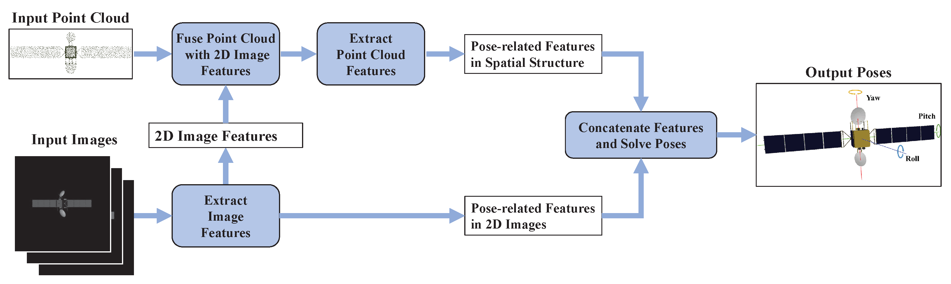
  • We propose a novel CNN-based satellite pose estimation method. The method takes full advantage of CNN and combines the spatial structure a priori information in the form of point clouds and accomplishes the task of estimating the relative pose of a satellite from a single monocular optical image with a high precision.
  • We design a loss function that is suitable for satellite pose estimation. The loss function can guide the network training process and make the pose estimation results more accurate.
  • We build an open-source simulation dataset called BUAA-SID-POSE 1.0. The dataset contains more than 250,000 images of five types of satellites in different poses, providing a large amount of data for relevant research.
The structure of this paper is as follows: Section 2 describes the related work of space object pose estimation; Section 3 describes the framework of the CNN architecture; Section 4 describes the dataset, experimental environment, evaluation metrics, and training strategy; Section 5 describes and analyzes the experimental results; and Section 6 presents the conclusions from this study.

2. Related Work

Template matching method: Template matching is a traditional pattern recognition method with simple implementation and strong interpretability. To estimate the pose of an input image, the general idea based on the template matching method is to project the 3D model from different perspectives to 2D images, then extract features from images or directly use the projected 2D image as a template, and finally use the matching method to find the template with the highest similarity to the input image. The pose of the input image is assigned to the pose of the matched template. Refs. [14,15,16,17] utilize the template matching method to estimate the pose of space objects and make various improvements. Ref. [26] first utilizes template matching as a coarse procedure, then establishes many-to-one 2D–3D correspondences by contour feature matching to obtain an accurate pose. In the ideal scenario, this kind of method can directly establish the correspondence between the pose and the template, but the template matching method has some problems, such as poor robustness and the contradiction between accuracy and speed.
Learning-based method: The general idea of the learning-based method is to extract features from images with pose labels and train a classifier or regressor to learn the mapping from features to poses, then extract features and solve the pose from the test images. There are also two ways to solve the pose. One is to establish a feature-keypoint mapping, confirm the location of the keypoints and solve the pose through the PnP algorithm, which is a classical 2D–3D matching method. The other is to establish the feature-pose mapping directly and obtain the corresponding pose of the image through the classifier or regressor. There is a lot of work investigating the use of learning-based methods to estimate the pose of space objects. Refs. [18,19,20,23] mainly use artificially extracted features to train classifiers in the offline stage and solve the pose in the online stage. Refs. [21,22] apply deep learning in pose estimation tasks and completes automatic feature extraction and pose calculation through an end-to-end network. Refs. [9,24,25,27,28] also apply deep learning, but these methods learn to locate keypoints and solve the pose through the PnP algorithm. The performance of learning-based methods depends on features. Good features can improve the performance of the algorithm, but artificially extracting features is a difficult job and the generalization of the features is poor. Although deep-learning-based pose estimation methods can automatically extract robust features, this method still has the problem of poor interpretability, and it is also difficult to obtain a large amount of labeled data.
The method of combining the 3D model: 3D models can represent the spatial structure of objects. Two-dimensional images corresponding to the target pose can be obtained by rendering the 3D model. The typical idea of utilizing a 3D model in general pose estimation can be divided into the following two kinds:
  • Refining the obtained pose solution [35].
  • Generating 2D–3D correspondence [36].
For satellites, Refs. [24,25] locate keypoints on sequence images by rendering a 3D model. These methods train a keypoint location network and solve the pose by RANSACK-PnP algorithms. Three-dimensional models are mainly used for generating 2D–3D matching. These methods are not end-to-end, and the RANSACK-PnP algorithm is time-consuming.
Different from these methods, this paper proposes to combine the 3D model represented by the point cloud into the network. Since point cloud data cannot reflect any features related to attitude, this paper extracts the features related to the pose through convolution and fuses them with point cloud data. Then features are extracted from the point cloud data. The entire network is end-to-end and does not require RANSACK-PnP or additional post-processing steps.

3. Method

The overall structure of the proposed method is shown in Figure 2. The structure can be divided into three modules. The first module is the feature extraction module, utilizing CNN to obtain the feature map from the input image. The second module is the 3D prior information fusion module, which consists of two branches. One branch extracts the feature vectors corresponding to 2D images; the other branch extracts the feature vectors related to the spatial structure from the 3D model. Finally, the features extracted by the two branches are concatenated. The third module is the pose solution module, solving the pose from features outputted from the second module. In this section, we will describe each module in detail.

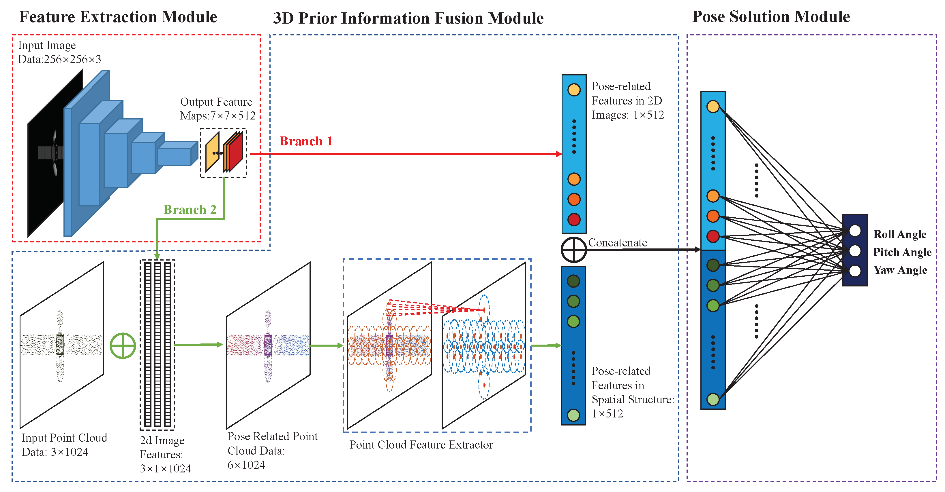
3.1. Feature Extraction Module

Feature extraction is an important step in the learning-based method. The convolutional neural network is used for feature extraction in pose estimation tasks because CNN has a strong feature extraction ability.
In this paper, we select the classic CNN structure ResNet [37] as the feature extractor. The structure of the feature extraction module is shown in Figure 3. The input image of ResNet is a three-channel image with the size of 224 × 224 × 3, but the images in our dataset have one channel with the size of 256 × 256 × 1. Therefore, we resize the original image to the target size via the interpolation method, and the gray image is copied into a three-channel image. Customizing the first convolution layer for a single-channel image is another alternative solution, but in order to retain the original network structure and to make the structure applicable to a three-channel image, we choose to change the channel of the input image. The output of the network is 7 × 7 × 512 feature maps.
In view of the small image size and the simple background, the network does not need to be very deep, so we choose a lighter network, ResNet18, as the feature extraction module. It should be mentioned that we initialize the network parameters in a random way. We show the relevant experimental results in Section 5.2.

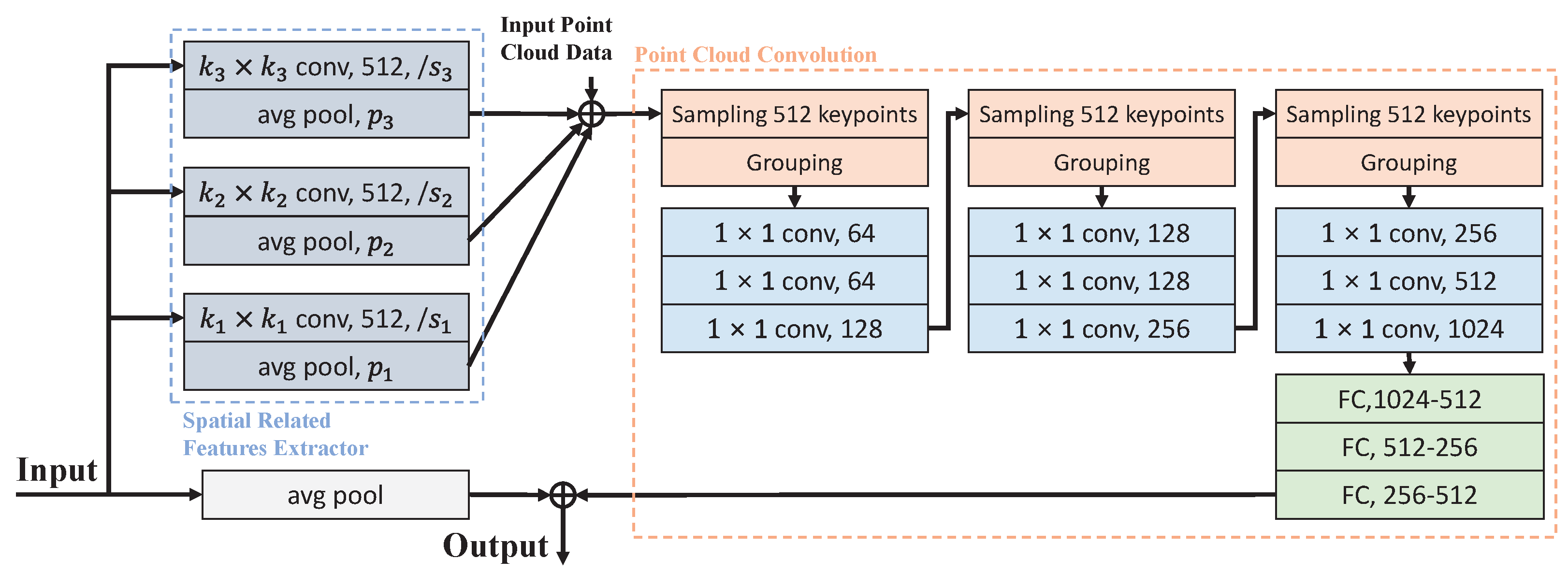
3.2. Three-Dimensional Prior Information Fusion Module

The 3D prior information fusion module contains two branches. One branch generates the pose-related features in 2D images with the size of 1 × 512 utilizing an average pooling layer, while the other branch generates the pose-related features in spatial structure with the size of 1 × 512 by the following steps. First, we extract features from the 2D image that correlate with the spatial structure. Then we fuse the features and 3D point cloud data by concatenating. Finally, we use the point cloud convolution method to receive the pose-related features of the spatial structure. After feature extraction, we concatenate these features together and form a 1024-d joint representation as the output of this module. The structure of the module is shown in Figure 4.
We utilize convolution to extract features from 2D images that correlate with the spatial structure. Through three parallel convolution layers, batch normalization layers, and maximum pooling layers, we obtain three 1024-d features. We concatenate these features with the point cloud matrix, which has the size of 1024 × 3 and receive the pose-related point cloud data with the size of 1024 × 6.
We choose PointNet++ [34] as the point cloud feature extractor. PointNet++ is developed from PointNet [33], which is a very classic point cloud convolution method with a simple structure. PointNet and PointNet++ have been proven to be effective in point cloud classification, point cloud component segmentation, and other applications.
PointNet first maps the points in the point cloud and then uses symmetric functions to solve the disorder problem. Before feature extraction, PointNet aligns all inputs by training affine transformation matrices. PointNet++ is an improved version of PointNet, which divides point cloud data into overlapping local regions by using the distance measurement of the space. First, local features are extracted from a small range of geometric structures. Then high-level features are extracted based on low-level local features. PointNet++ divides point cloud data by query ball, and each query ball is determined by the center coordinate and radius, such as the convolution kernel in CNN, where the center coordinate is the position of the convolution kernel and the radius is the size of the convolution kernel.
SSG (single-scale grouping) and MSG (multi-scale grouping) are two ways to extract local features in PointNet++. SSG takes query balls of the same radius for each centroid of the current layer and extracts single-scale features, while MSG takes query balls with different radii for each centroid of the current layer, extracts features for these query balls separately, and concatenates them as the output to extract multi-scale features. The specific structure of SSG and MSG can be found in [34].
Relevant experiments on this module will be shown in Section 5.3.

3.3. Pose Solution Module

In the pose solution module, we estimated the pitch angle, yaw angle, and roll angle at the same time. The range of the pitch angle is [−90 , +90 ], the range of the yaw angle is (−180 , +180 ], and the range of the roll angle is [0 , 360 ). In this module, we use full connection layers to solve the pose from the output of the 3D prior information fusion module. We output a 3D vector, and the three dimensions represent pitch angle, yaw angle, and roll angle, respectively.
In the training process, we design the rotation-normalized L2 loss. The loss function is defined as follows,
L = L 1 w 1 + L 2 w 2 + L 3 w 3
where L 1 w 1 , L 2 w 2 , and L 3 w 3 represent the loss of pitch angle, yaw angle, and roll angle, respectively, which are defined as follows,
L 1 w 1 = w 1 · g f 1 y 1 f 1 x 1 L 2 w 2 = w 2 · g min f 2 y 2 f 2 x 2 , 2 f 2 y 2 f 2 x 2 L 3 w 3 = w 3 · g min f 3 y 3 f 3 x 3 , 2 f 3 y 3 f 3 x 3
where y 1 , y 2 , y 3 , x 1 , x 2 , and x 3 represent the ground truth and the prediction of the pitch angle, yaw angle, and roll angle, respectively, and f 1 · , f 2 · , and f 3 · represent the normalized function of the pitch angle, yaw angle, and roll angle; defined as follows,
f 1 x = x / 90 f 2 x = x / 180 f 3 x = x / 360
where g · represents the post-processing function, such as square function, linear function, logarithmic function, etc. w 1 , w 2 , and w 3 represent the weight of pitch angle, yaw angle, and roll angle in the loss function. Through experimenting, we selected the settings as Equations (4) and (5) for the network. The experimental results are shown in Section 5.1.
g x = log 2 2 x + 1
w 1 = 1.3 , w 2 = 0.4 , w 3 = 1.3

4. Experiment Settings
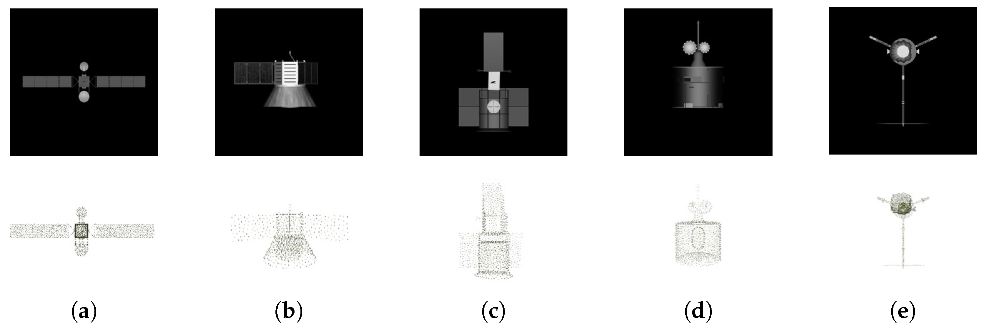
4.1. Dataset

BUAA-SID-POSE 1.0: We built a simulation dataset called BUAA-SID-POSE 1.0. BUAA-SID-POSE 1.0 is an extension based on BUAA-SID 1.0 [19,38,39], and their simulation methods are the same. Compared with BUAA-SID 1.0, BUAA-SID-POSE 1.0 not only collects more intensive samples on the viewpoint sphere but also adds the roll of the camera. The yaw angle ranges from −180 to 180 , and samples are taken every 3 . The pitch angle ranges from −90 to 90 , and samples are taken every 3 . Because there is only one viewpoint at 90 north latitude and 90 south latitude, a total of 118 × 60 + 2 = 7082 viewpoints are sampled. For each viewpoint, we sample the camera roll angle every 45 within the range of [0 , 360 ). To avoid the influence of other factors, we stay at the same position from the light source relative to the camera and the same camera distance from the satellite.
BUAA-SID-POSE 1.0 includes five satellites with significantly different appearances, as shown in Table 1.
When experimenting, we randomly divide BUAA-SID-POSE 1.0 into train set:valuation set:test set = 1:1:18. The image number of the train set and the valuation set is 2832, and the number of the test set is 50,992.
Point cloud data acquisition: The 3D model of the satellite is stored as a unit of triangles, but our proposed method expresses the 3D model through the form of the point cloud. Therefore, we obtain point cloud data by constrained Poisson–Disk Sampling [40]. This method can generate uniformly distributed point cloud data on the surface of the model, which is beneficial to the subsequent operation.
At this stage, we extract the point cloud with a point number of more than 1024, and different models have different point numbers. To standardize the input, we sample the point cloud utilizing the farthest point sample method. The point cloud generated is a matrix with the size of 1024 × 3.
The simulated satellite images and point cloud extraction results are shown in Figure 5.

4.2. Experimental Environment

The software environment used in the experiment is as follows: The operating system is Ubuntu16.0, the programming environment is PyCharm, the language is Python and the version is Python3.7, and the deep learning framework is PyTorch1.4.
The hardware used in the experiment is as follows: The code runs on a server with Intel(R) Xeon(R)Silver 4114 CPU @ 2.20 GHz. The neural network is trained and tested using a GTX 2080Ti GPU with 12 GB video memory.

4.3. Evaluation Metrics

Referring to [19,20], we calculate the following indexes:
  • Mean Absolute Error (MAE): MAE evaluates the mean error between the predicted pose and the ground truth. The calculation formula is shown as follows,
    M A E = 1 N i = 0 N 1 y p r e d y t r u t h
  • Accuracy Rate (ACC): ACC evaluates the accuracy of the results under different accuracy requirements, including the ACC with the absolute error of less than 1 and less than 5 denoted by A C C ( A E < 1 ) and A C C ( A E < 5 ) . AE is the absolute value of the difference between the predicted value and the true value. Considering the reasonableness of the absolute error threshold size settings in the metric, we examined the relevant literature. Ref. [21] uses a classification scheme to estimate the pose with a resolution much greater than 5 in yaw angle, pitch angle, and roll angle; Ref. [9] also estimates attitude using a classification scheme with a resolution of 10 in each dimension. In summary, the absolute error threshold chosen for the evaluation metrics is quite accurate when comparing existing algorithms for space object pose estimation.
We calculate M A E , A C C ( A E < 1 ), and A C C ( A E < 5 ) for yaw angle α , pitch angle β , and roll angle γ , including nine evaluation metrics in total.

4.4. Training Strategy

During training, when all the images in the training set are used to train the neural network, it is said to have completed an epoch of training. A reasonable number of epochs can ensure sufficient convergence of the model while reducing the training time. We ensure that the model converges sufficiently by observing the loss descent curve on the validation set.
We optimize the network using a common optimization algorithm, stochastic gradient descent (SGD) with momentum, with the initial learning rate set to 0.1 and the momentum set to 0.9. We use a step learning rate decline schedule to ensure the network convergence, the learning rate decreases to 1/10 of the original rate after each certain number of epochs. At the same time, we use the warm-up strategy to avoid network divergence at the beginning of training.
Considering the randomness in the training process of the convolution neural network and the randomness in the division of the dataset, we use randomized repeat experiments to reduce the interference caused by randomness. We used a completely random approach for the three dataset divisions, training the model three times on each dataset and generating the results. In this way, we run nine repeat experiments for each setup in total, with the mean of the results being the final experimental result and the variance being the uncertainty of the results.

5. Experimental Results

5.1. Experimental Results of the Loss Function

We study the loss function, which was defined in Section 3.3, focusing on the form of g · , and the values of w 1 , w 2 , and w 3 . The experimental settings are shown in Table 2.
With representativeness, we used the A2100 satellite model for training and testing and tested the loss function without using the 3D model. We divided the dataset as train set:validation set:test set = 6:2:2. We trained 32 epochs to ensure full convergence of the model, the first three epochs were the warm-up phase, and the learning rate was decreased every eight epochs. The batch size was chosen as 128.
As shown in Table 3, it can be found that g ( x ) = x 2 leads to poorer experimental results, mainly because the angles have been normalized before calculating the loss, and when the predicted value is closer to the ground truth, the error will be very small, leading to a decrease in the model’s ability to further learn more accurate poses, especially in A C C ( A E < 1 ) , the metric reflecting high precision forecasting capability. In contrast, as can be seen in Figure 6, log 2 2 x + 1 better amplifies the error value when the predicted value is closer to the ground truth, which guides the network to learn a more accurate pose.
For the values of w 1 , w 2 , and w 3 , we adapt them based on the L3 setting. As the network is more capable of estimating the pitch angle, we reduce the weight of the pitch angle error in the total error. We find that the metrics irrelevant to pitch angle are generally higher in the L4 setting, and the degradation of the metrics related to the pitch angle is within acceptable limits.

5.2. Experimental Results of Model Structure and Initialization Mode

We experimented with the influence of model structure and the initialization mode of CNN. With representativeness, the experimental setting was the same as in Section 5.1. We compare the influence of the channel number on the input image. As shown in Table 4, inputting a one-channel image and customizing the C1 layer yields similar results to copying the one-channel image to generate a three-channel image, and these two methods have similar model size as well, which indicates that there is no major effect on the experimental results on different input strategies.
We also compared the pose estimation metrics between ResNet18 and ResNet50. We also tested the model performance with and without the pretrained model and the influence of the image channel. The pretrained model was trained on the natural image dataset ImageNet [41]. The network that inputs a three-channel image freezes layers C1 and C2 in Figure 3, while the network that inputs a one-channel image reinitializes the parameter in layer C1 and freezes the parameters in layers C2 and C3. When not using the pretrained model, we adopted the random initialization method.
As shown in Table 5, using the pretrained models is less effective compared to the random initialization. This phenomenon suggests that the simulated dataset used in this experiment has a large gap compared to the natural conditions dataset, and the network parameters cannot be shared. The pretrained model that inputs a one-channel image is less effective than the pretrained model that inputs a three-channel image, mainly because randomly initializing the first convolutional layer and freezing subsequent convolutional layers makes training more difficult and less stable, and Setting 3 has more frozen parameters than Setting 2. This also supports the conclusion that there is a gap between the different datasets. With the random initialization method, ResNet50 achieves better performance than ResNet18, but the improvement was not significant. This phenomenon suggests that deepening the network depth can improve the accuracy of the algorithm, but ResNet18 already has a strong feature extraction capability. Taking performance and speed into account, we choose ResNet18 as the feature extraction module of the network.

5.3. Experimental Results from the Structures of 3D Prior Information Fusion Module

We experimented with the different implementation details of the 3D prior information fusion module. We tested different structures of the point cloud convolution network and the structures of related spatial features extractor in Figure 4. The experimental settings are shown in Table 6.
To prove the validity of the 3D prior information fusion module, we also tested the performance of the network without the 3D prior information fusion module. The result is shown in Table 7 as “Compare”.
We performed the experiment with the A2100 satellite model. We trained 300 epochs to ensure full convergence of the model, the first 10 epochs were the warm-up phase, and the learning rate decreased every 90 epochs. S5 and S6 chose the batch size as 16 while the other settings chose the batch size as 64.
As shown in Table 7, the 3D prior information fusion module can significantly improve performance. The PointNet network structure improves the results less and even decreases the accuracy of the pitch angle. We believe that this is due to PointNet focus on the overall point cloud information and has little ability to extract features from the local area. PointNet is not suitable in 3D prior information fusion modules.
Overall, for all of the experimental settings using PointNet++, the improvement of MSG is more obvious than SSG. We believe that the MSG structure can extract more complex and reasonable features from the local area, which has a greater impact on the model performance. From the experimental results, we can conclude that MSG can achieve more accurate poses.
For different structures of the convolutional layer, we find that the results are better in MSG with the different kernel size settings of convolutional layers. while the opposite is true for the SSG structure. We think that this is because MSG is more capable of handling features with different scales than SSG. The features extracted by convolution with different kernel sizes have multi-scale characteristics, and the operation of extracting and combining features from multiple radius query balls in MSG is better adapted to the case of input multi-scale features.
Collectively, we suggest that the experimental setup of S6 can obtain the best results.

5.4. Pose Estimation Results on BUAA-SID-POSE 1.0

We tested the method on BUAA-SID-POSE 1.0. We trained a separate set of neural network parameters for each type of satellite. In the course of each training, we trained 300 epochs to ensure full convergence of the model, the first 10 epochs were the warm-up phase, and the learning rate decreased every 90 epochs.
As shown in Table 8, the proposed methods have different abilities for estimating the pose of different satellites. In general, the network structure is generally less capable of estimating the yaw angle of the satellite and more capable of estimating the pitch and roll angles.
For the A2100 satellite, which has two solar wings with a symmetric distribution and a certain symmetry in two dimensions, the network is less effective in the roll and pitch angle estimation tasks and more effective in the yaw angle recognition. For the COBE satellite, which has three solar wings equally spaced in a circular shape on one side of the cylindrical satellite body, the network is less effective in the yaw angle recognition and more effective in the other two angles. For EARLY-BIRD, a satellite with poor symmetry, the network has a better pose recognition ability and achieves the best performance in yaw angle recognition. Compared to other satellites, for FENGYUN, a satellite with a cylindrical body and no extended solar wings, the pose estimation accuracy is high, except for the yaw angle. For GALILEO satellites, which have a long pole structure with a certain degree of centrosymmetry, the network has better performance in roll angle and poorer performance in the other two angles.
From the above analysis, it can be seen that the pose attitude capability varies widely for different satellite models, and for the poses with less symmetry, the network performs better. The symmetry of the satellite model has a large impact on the network performance, and the pose estimation ability can be further improved by considering the symmetry.

5.5. Comparison

Finally, we compared the method proposed in this paper with the benchmark method using deep learning. We used the same feature extraction network as this paper and regressed the pose directly from the output of the feature extraction network. We supervised the network using the loss function proposed in Section 3.3. This approach to pose estimation is very similar to [21] but differs in the presentation of the pose. The training details of the two methods were consistent. The mean evaluation on BUAA-SID-POSE 1.0 of our method and the typical pose regression method is shown in Table 9.
Our method outperforms the typical deep-learning-based pose estimation methods in a variety of metrics, which demonstrates that using the 3D model as a priori information can effectively improve the accuracy of pose estimation. There is a large improvement in the metrics related to the roll angle and pitch angle, but the improvement in the metrics related to yaw angle is not significant. This is mainly because the method proposed in this paper does not have a good way to deal with symmetry, which is the main reason for the low detection accuracy in this dimension of yaw angle.

6. Conclusions

In this paper, we design a novel network that uses a monocular 2D visible image to estimate the pose of space objects combined with a 3D model as a priori information. The utilization of 3D prior information is realized by the point cloud convolution method. We also designed a loss function dedicated to the space object pose estimation according to the characteristics of the task. We build a simulation dataset, including five satellite models, called BUAA-SID-POSE 1.0 and perform experiments on it. We achieve 71%, 94%, and 95% accuracy for yaw angle, pitch angle, and roll angle with an error of fewer than five degrees, respectively. The proposed method can meet the requirements of satellite pose estimation tasks and make a contribution to the field of intelligent spaceflight.

Author Contributions

Conceptualization, S.Q., H.Z., G.M., M.A., F.X. and Z.J.; methodology, S.Q. and H.Z.; software, S.Q.; validation, S.Q., H.Z. and F.X.; formal analysis, S.Q.; investigation, S.Q.; resources, G.M., M.A. and H.Z.; data curation, S.Q. and H.Z.; writing—original draft preparation, S.Q.; writing—review and editing, S.Q., H.Z., G.M. and M.A.; visualization, S.Q.; supervision, H.Z.; project administration, H.Z.; funding acquisition, H.Z. All authors have read and agreed to the published version of the manuscript.

Funding

This work was supported in part by the Fundamental Research Funds for the Central Universities.

Institutional Review Board Statement

Not applicable.

Informed Consent Statement

Not applicable.

Data Availability Statement

The BUAA-SID-POSE1.0 dataset presented in this study is openly available at https://www.kaggle.com/datasets/qiaosijia/buaa-sid-pose-1 (accessed on 25 October 2022).

Conflicts of Interest

The authors declare no conflict of interest. The funders had no role in the design of the study; in the collection, analyses, or interpretation of data; in the writing of the manuscript, or in the decision to publish the results.

References

  1. Zhang, L.; Zhang, S.; Yang, H.; Cai, H.; Qian, S. Relative attitude and position estimation for a tumbling spacecraft. Aerosp. Sci. Technol. 2015, 42, 97–105. [Google Scholar] [CrossRef]
  2. Flores-Abad, A.; Ma, O.; Pham, K.; Ulrich, S. A review of space robotics technologies for on-orbit servicing. Prog. Aerosp. Sci. 2014, 68, 1–26. [Google Scholar] [CrossRef] [Green Version]
  3. Long, A.; Richards, M.; Hastings, D.E. On-Orbit Servicing: A New Value Proposition for Satellite Design and Operation. J. Spacecr. Rocket. 2007, 44, 964–976. [Google Scholar] [CrossRef] [Green Version]
  4. Ambrose, R.; Nesnas, I.; Chandler, F.; Allen, B.; Fong, T.; Matthies, L.; Mueller, R. NASA Technology Roadmaps: TA 4: Robotics and Autonomous Systems; NASA: Washington DC, USA, 2015; pp. 50–51. [Google Scholar]
  5. Li, Y.; Zhang, A. Observability analysis and autonomous navigation for two satellites with relative position measurements. Acta Astronaut. 2019, 163, 77–86. [Google Scholar] [CrossRef]
  6. Pinard, D.; Reynaud, S.; Delpy, P.; Strandmoe, S.E. Accurate and autonomous navigation for the ATV. Aerosp. Sci. Technol. 2007, 11, 490–498. [Google Scholar] [CrossRef]
  7. Xing, Y.; Cao, X.; Zhang, S.; Guo, H.; Wang, F. Relative position and attitude estimation for satellite formation with coupled translational and rotational dynamics. Acta Astronaut. 2010, 67, 455–467. [Google Scholar] [CrossRef]
  8. De Jongh, W.; Jordaan, H.; Van Daalen, C. Experiment for pose estimation of uncooperative space debris using stereo vision. Acta Astronaut. 2020, 168, 164–173. [Google Scholar] [CrossRef]
  9. Cassinis, L.P.; Fonod, R.; Gill, E.; Ahrns, I.; Gil-Fernández, J. Evaluation of tightly-and loosely-coupled approaches in CNN-based pose estimation systems for uncooperative spacecraft. Acta Astronaut. 2021, 182, 189–202. [Google Scholar] [CrossRef]
  10. Guthrie, B.; Kim, M.; Urrutxua, H.; Hare, J. Image-based attitude determination of co-orbiting satellites using deep learning technologies. Aerosp. Sci. Technol. 2022, 120, 107232. [Google Scholar] [CrossRef]
  11. Ventura, J. Autonomous Proximity Operations for Noncooperative Space Targets. Ph.D. Thesis, Technische Universität München, Munich, Germany, 2016. [Google Scholar]
  12. Sharma, S.; Ventura, J.; D’Amico, S. Robust model-based monocular pose initialization for noncooperative spacecraft rendezvous. J. Spacecr. Rocket. 2018, 55, 1414–1429. [Google Scholar] [CrossRef]
  13. Pesce, V.; Haydar, M.F.; Lavagna, M.; Lovera, M. Comparison of filtering techniques for relative attitude estimation of uncooperative space objects. Aerosp. Sci. Technol. 2019, 84, 318–328. [Google Scholar] [CrossRef]
  14. Petit, A.; Marchand, E.; Kanani, K. Vision-based detection and tracking for space navigation in a rendezvous context. In Proceedings of the International Symposium on Artificial Intelligence, Robotics and Automation in Space i-SAIRAS 2012, Turin, Italy, 4–6 September 2012. [Google Scholar]
  15. Opromolla, R.; Fasano, G.; Rufino, G.; Grassi, M. A model-based 3D template matching technique for pose acquisition of an uncooperative space object. Sensors 2015, 15, 6360–6382. [Google Scholar] [CrossRef] [PubMed] [Green Version]
  16. Opromolla, R.; Fasano, G.; Rufino, G.; Grassi, M. Pose estimation for spacecraft relative navigation using model-based algorithms. IEEE Trans. Aerosp. Electron. Syst. 2017, 53, 431–447. [Google Scholar] [CrossRef]
  17. Yin, F.; Chou, W.; Wu, Y.; Dong, M. Relative pose determination of uncooperative known target based on extracting region of interest. Meas. Control 2020, 53, 589–600. [Google Scholar] [CrossRef]
  18. Zhang, H.; Jiang, Z.; Elgammal, A. Vision-based pose estimation for cooperative space objects. Acta Astronaut. 2013, 91, 115–122. [Google Scholar] [CrossRef]
  19. Zhang, H.; Jiang, Z. Multi-view space object recognition and pose estimation based on kernel regression. Chin. J. Aeronaut. 2014, 27, 1233–1241. [Google Scholar] [CrossRef] [Green Version]
  20. Zhang, H.; Jiang, Z.; Yao, Y.; Meng, G. Vision-based pose estimation for space objects by Gaussian process regression. In Proceedings of the 2015 IEEE Aerospace Conference, Big Sky, MT, USA, 7–14 March 2015; pp. 1–9. [Google Scholar]
  21. Sharma, S.; Beierle, C.; D’Amico, S. Pose estimation for non-cooperative spacecraft rendezvous using convolutional neural networks. In Proceedings of the 2018 IEEE Aerospace Conference, Big Sky, MT, USA, 3–10 March 2018; pp. 1–12. [Google Scholar]
  22. Phisannupawong, T.; Kamsing, P.; Torteeka, P.; Channumsin, S.; Sawangwit, U.; Hematulin, W.; Jarawan, T.; Somjit, T.; Yooyen, S.; Delahaye, D.; et al. Vision-Based Spacecraft Pose Estimation via a Deep Convolutional Neural Network for Noncooperative Docking Operations. Aerospace 2020, 7, 126. [Google Scholar] [CrossRef]
  23. Oumer, N.W.; Kriegel, S.; Ali, H.; Reinartz, P. Appearance learning for 3D pose detection of a satellite at close-range. ISPRS J. Photogramm. Remote. Sens. 2017, 125, 1–15. [Google Scholar] [CrossRef] [Green Version]
  24. Chen, B.; Cao, J.; Parra, A.; Chin, T.J. Satellite Pose Estimation with Deep Landmark Regression and Nonlinear Pose Refinement. In Proceedings of the 2019 IEEE/CVF International Conference on Computer Vision Workshop, Seoul, Republic of Korea, 27–28 October 2019; pp. 2816–2824. [Google Scholar]
  25. Huo, Y.; Li, Z.; Zhang, F. Fast and accurate spacecraft pose estimation from single shot space imagery using box reliability and keypoints existence judgments. IEEE Access 2020, 8, 216283–216297. [Google Scholar] [CrossRef]
  26. Zhang, X.; Jiang, Z.; Zhang, H.; Wei, Q. Vision-Based Pose Estimation for Textureless Space Objects by Contour Points Matching. IEEE Trans. Aerosp. Electron. Syst. 2018, 54, 2342–2355. [Google Scholar] [CrossRef]
  27. Pasqualetto Cassinis, L.; Menicucci, A.; Gill, E.; Ahrns, I.; Sanchez-Gestido, M. On-ground validation of a CNN-based monocular pose estimation system for uncooperative spacecraft: Bridging domain shift in rendezvous scenarios. Acta Astronaut. 2022, 196, 123–138. [Google Scholar] [CrossRef]
  28. Li, K.; Zhang, H.; Hu, C. Learning-Based Pose Estimation of Non-Cooperative Spacecrafts with Uncertainty Prediction. Aerospace 2022, 9, 592. [Google Scholar] [CrossRef]
  29. Liu, Y.; Huang, T.S.; Faugeras, O.D. Determination of camera location from 2-D to 3-D line and point correspondences. IEEE Trans. Pattern Anal. Mach. Intell. 1990, 12, 28–37. [Google Scholar] [CrossRef]
  30. Shiu, Y.C.; Ahmad, S. 3D location of circular and spherical features by monocular model-based vision. In Proceedings of the IEEE International Conference on Systems, Man and Cybernetics, Cambridge, MA, USA, 14–17 November 1989; pp. 576–581. [Google Scholar]
  31. Meng, C.; Xue, J.; Hu, Z. Monocular Position-Pose Measurement Based on Circular and Linear Features. In Proceedings of the 2015 International Conference on Digital Image Computing: Techniques and Applications (DICTA), Adelaide, Australia, 23–25 November 2015; pp. 1–8. [Google Scholar]
  32. Meng, C.; Li, Z.; Sun, H.; Yuan, D.; Bai, X.; Zhou, F. Satellite Pose Estimation via Single Perspective Circle and Line. IEEE Trans. Aerosp. Electron. Syst. 2018, 54, 3084–3095. [Google Scholar] [CrossRef]
  33. Qi, C.R.; Su, H.; Mo, K.; Guibas, L.J. Pointnet: Deep learning on point sets for 3d classification and segmentation. In Proceedings of the IEEE Conference on Computer Vision and Pattern Recognition, Honolulu, HI, USA, 21–26 July 2017; pp. 652–660. [Google Scholar]
  34. Qi, C.R.; Yi, L.; Su, H.; Guibas, L.J. Pointnet++: Deep hierarchical feature learning on point sets in a metric space. In Proceedings of the 31st International Conference on Neural Information Processing Systems (NIPS 2017), Long Beach, CA, USA, 4–9 December 2017; pp. 5105–5114. [Google Scholar]
  35. Manhardt, F.; Kehl, W.; Navab, N.; Tombari, F. Deep model-based 6d pose refinement in rgb. In Proceedings of the European Conference on Computer Vision, Munich, Germany, 8–14 September 2018; pp. 800–815. [Google Scholar]
  36. Wang, Y.; Tan, X.; Yang, Y.; Liu, X.; Ding, E.; Zhou, F.; Davis, L.S. 3d pose estimation for fine-grained object categories. In Proceedings of the European Conference on Computer Vision Workshops, Munich, Germany, 8–14 September 2018; pp. 619–632. [Google Scholar]
  37. He, K.; Zhang, X.; Ren, S.; Sun, J. Deep residual learning for image recognition. In Proceedings of the IEEE Conference on Computer Vision and Pattern Recognition, Las Vegas, NV, USA, 26 June–1 July 2016; pp. 770–778. [Google Scholar]
  38. Zhang, H.; Liu, Z.; Jiang, Z.; An, M.; Zhao, D. BUAA-SID1.0 space object image dataset. Spacecr. Recovery Remote. Sens. 2010, 31, 65–71. [Google Scholar]
  39. Meng, G.; Jiang, Z.; Liu, Z.; Zhang, H.; Zhao, D. Full-viewpoint 3D Space Object Recognition Based on Kernel Locality Preserving Projections. Chin. J. Aeronaut. 2010, 23, 563–572. [Google Scholar]
  40. Corsini, M.; Cignoni, P.; Scopigno, R. Efficient and flexible sampling with blue noise properties of triangular meshes. IEEE Trans. Vis. Comput. Graph. 2012, 18, 914–924. [Google Scholar] [CrossRef]
  41. Krizhevsky, A.; Sutskever, I.; Hinton, G. ImageNet Classification with Deep Convolutional Neural Networks. In Proceedings of the 25th International Conference on Neural Information Processing Systems, Red Hook, NY, USA, 3–6 December 2012; pp. 1097–1105. [Google Scholar]
Figure 1. The overall idea of the proposed method. First, we extract the features from the input image and get pose-related features in 2D images. Then, we fuse the point cloud data with 2D features extracted from the image and obtain the pose-related features in the spatial structure. Finally, we concatenate the features together and solve the pose.
Aerospace 09 00768 g001
Figure 2. The pipeline of the proposed method. First, we input the images to the features extraction module to extract the features. Then, we input features to the 3D prior information fusion module, which consists of two branches. Branch 1, shown in red lines, extracts the features corresponding to the 2D images. Branch 2, shown in green lines, extracts the features related to the spatial structure by combining the 3D model. The features extracted by the two branches are concatenated. Finally, the concatenated module is input to the pose solution module to solve the pose.
Aerospace 09 00768 g002
Figure 3. The structure of the feature extraction module. k × k c o n v , n means the kernel size of the convolution layer is k and the kernel number of the convolution layer is n, while / p means the stride of the convolution layer is p. Different colors represent different layers.
Aerospace 09 00768 g003
Figure 4. The structure of the 3D Prior Information Fusion Module. k × k c o n v , n , / s means the convolution layer with the kernel size of k, the kernel number of n, and the stride of s, while p means the pooling layer with a stride of p. F C , n 1 n 2 means the input and the output of the connection layer are n 1 and n 2 , respectively.
Aerospace 09 00768 g004
Figure 5. Simulated satellite images and corresponding point cloud. (a) A2100; (b) COBE; (c) EARLY-BIRD; (d) DSP; (e) GALILEO.
Aerospace 09 00768 g005
Figure 6. Values of different g · in the range [0, 1]. (a) g ( x ) = x 2 ; (b) g ( x ) = x ; (c) g ( x ) = log 2 2 x + 1 .
Aerospace 09 00768 g006
Table 1. The description of the satellites in BUAA-SID-POSE 1.0.
TypeApperance
A2100Has a pair of solar wings, which are symmetrically placed on both sides of the cube’s body
COBEHas three solar wings, which are placed around the cylindrical body evenly.
EARLY-BIRDHas two solar wings, which are distributed on the same side of the body.
FENGYUNHas an entirely cylindrical satellite.
GALILEOHas three long pole structures distributed around the body.
Table 2. The settings of the loss function.
N.O. w 1 w 2 w 3 g ·
L1111 x 2
L2111 x
L3111 log 2 2 x + 1
L41.30.41.3 log 2 2 x + 1
Table 3. Performance of different loss function settings. The optimal results are tabulated in red.
Evaluation MetricExperimental Setting
L1L2L3L4
α _ A C C ( A E < 1 ) 0.220 ± 0.0360.495 ± 0.0280.550 ± 0.0320.557 ± 0.028
β _ A C C ( A E < 1 ) 0.388 ± 0.0200.883 ± 0.0090.912 ± 0.0120.737 ± 0.023
γ _ A C C ( A E < 1 ) 0.292 ± 0.0420.522 ± 0.0680.560 ± 0.0610.648 ± 0.052
α _ A C C ( A E < 5 ) 0.637 ± 0.0460.941 ± 0.0090.936 ± 0.0210.941 ± 0.016
β _ A C C ( A E < 5 ) 0.967 ± 0.0070.999 ± 0.0000.999 ± 0.0000.998 ± 0.000
γ _ A C C ( A E < 5 ) 0.600 ± 0.0280.924 ± 0.0180.925 ± 0.0300.948 ± 0.014
α _ M A E 6.27 ± 0.532.31 ± 0.2432.32 ± 0.592.22 ± 0.35
β _ M A E 1.72 ± 0.110.56 ± 0.020.51 ± 0.030.81 ± 0.05
γ _ M A E 7.91 ± 0.403.12 ± 0.453.05 ± 0.852.32 ± 0.45
Table 4. The influence of the channel number of the input image.
Experimental SettingEvaluation Metric
α _ ACC
( AE < 5 )
β _ ACC
( AE < 5 )
γ _ ACC
( AE < 5 )
α _ MAE β _ MAE γ _ MAE Model Size
Copy one-channel image to generate three-channel image0.941 ± 0.0160.998 ± 0.0000.948 ± 0.0142.223 ± 0.3520.806 ± 0.0502.316 ± 0.45242.70 MB
Input one-channel image and customize layer C10.938 ± 0.0220.995 ± 0.0010.944 ± 0.0192.333 ± 0.5870.919 ± 0.6122.560 ± 0.54842.68 MB
Table 5. Performance of different model structures and initialization mode analysis. The optimal results are tabulated in red.
Evaluation MetricExperimental Setting *
ResNet18
Setting 1
ResNet18
Setting 2
ResNet18
Setting 3
ResNet50
Setting 1
ResNet50
Setting 2
ResNet50
Setting 3
α _ A C C ( A E < 1 ) 0.557 ± 0.0280.474 ± 0.0240.388 ± 0.0210.623 ± 0.0790.403 ± 0.0630.337 ± 0.061
β _ A C C ( A E < 1 ) 0.737 ± 0.0230.630 ± 0.0330.559 ± 0.0240.786 ± 0.0720.513 ± 0.1080.256 ± 0.114
γ _ A C C ( A E < 1 ) 0.648 ± 0.0520.591 ± 0.1180.558 ± 0.0570.649 ± 0.1930.187 ± 0.0990.238 ± 0.073
α _ A C C ( A E < 5 ) 0.941 ± 0.0160.897 ± 0.0190.884 ± 0.0100.971 ± 0.0050.907 ± 0.0320.828 ± 0.064
β _ A C C ( A E < 5 ) 0.998 ± 0.0000.995 ± 0.0020.985 ± 0.0020.998 ± 0.0000.990 ± 0.0750.785 ± 0.287
γ _ A C C ( A E < 5 ) 0.948 ± 0.0140.906 ± 0.0360.905 ± 0.0110.975 ± 0.0100.392 ± 0.2930.458 ± 0.328
α _ M A E 2.223 ± 0.3523.248 ± 0.6473.912 ± 0.2651.588 ± 0.2262.616 ± 0.5474.815 ± 2.546
β _ M A E 0.806 ± 0.0501.035 ± 0.0771.323 ± 0.0780.725 ± 0.1041.330 ± 0.3017.448 ± 13.529
γ _ M A E 2.316 ± 0.4523.353 ± 1.1483.955 ± 0.3461.392 ± 0.45845.055 ± 41.09243.644 ± 43.736
* Setting1 means no pretrained model is used, Setting 2 means using a pretrained model and the parameters of C1 and C2 are frozen, and Setting 3 means using a pretrained model but the input is a one-channel image, while the parameter of C1 is reinitialized and the parameters of C2 and C3 are frozen.
Table 6. The settings of the 3D prior information fusion module. Refer to Figure 4 for symbol meanings.
N.O.Structure of Point Cloud Convolution NetworkStructure of Spatial Related Features Extractor
S1PointNet k 1 , s 1 , p 1 = 3, 2, 3
k 2 , s 2 , p 2 = 3, 2, 3
k 3 , s 3 , p 3 = 3, 2, 3
S2PointNet++ (SSG) k 1 , s 1 , p 1 = 3, 2, 3
k 2 , s 2 , p 2 = 3, 2, 3
k 3 , s 3 , p 3 = 3, 2, 3
S3PointNet++ (SSG) k 1 , s 1 , p 1 = 3, 1, 5
k 2 , s 2 , p 2 = 3, 1, 5
k 3 , s 3 , p 3 = 3, 1, 5
S4PointNet++ (SSG) k 1 , s 1 , p 1 = 3, 1, 5
k 2 , s 2 , p 2 = 5, 1, 3
k 3 , s 3 , p 3 = 7, 1, 1
S5PointNet++ (MSG) k 1 , s 1 , p 1 = 3, 2, 3
k 2 , s 2 , p 2 = 3, 2, 3
k 3 , s 3 , p 3 = 3, 2, 3
S6PointNet++ (MSG) k 1 , s 1 , p 1 = 3, 1, 5
k 2 , s 2 , p 2 = 5, 1, 3
k 3 , s 3 , p 3 = 7, 1, 1
Table 7. Performance of different 3D prior information fusion module structures. The optimal results are tabulated in red.
Evaluation MetricExperimental Setting
CompareS1S2S3S4S5S6
α _ A C C ( A E < 1 ) 0.278 ± 0.0340.306 ± 0.0430.331 ± 0.0190.335 ± 0.0110.294 ± 0.0350.364 ± 0.0650.386 ± 0.033
β _ A C C ( A E < 1 ) 0.369 ± 0.0240.350 ± 0.1200.448 ± 0.0300.445 ± 0.0220.371 ± 0.0480.483 ± 0.0490.454 ± 0.035
γ _ A C C ( A E < 1 ) 0.370 ± 0.0600.439 ± 0.0660.645 ± 0.0730.458 ± 0.0640.350 ± 0.0720.563 ± 0.0560.560 ± 0.06
α _ A C C ( A E < 5 ) 0.699 ± 0.3170.730 ± 0.0500.745 ± 0.0240.756 ± 0.0120.711 ± 0.0320.765 ± 0.0430.773 ± 0.019
β _ A C C ( A E < 5 ) 0.849 ± 0.0170.785 ± 0.1620.901 ± 0.0270.893 ± 0.0210.864 ± 0.0250.892 ± 0.0170.891 ± 0.014
γ _ A C C ( A E < 5 ) 0.714 ± 0.0560.769 ± 0.0420.782 ± 0.0430.782 ± 0.0440.666 ± 0.1090.831 ± 0.0290.839 ± 0.022
α _MAE9.55 ± 1.418.16 ± 1.017.94 ± 1.007.48 ± 0.749.49 ± 1.617.54 ± 1.187.40 ± 0.75
β _MAE4.86 ± 0.495.12 ± 1.143.91 ± 0.654.02 ± 0.504.77 ± 0.494.34 ± 0.664.26 ± 0.30
γ _MAE11.48 ± 1.569.96 ± 0.489.63 ± 1.649.61 ± 1.5013.35 ± 3.499.05 ± 2.098.29 ± 1.04
Table 8. Performance on the BUAA-SID-POSE 1.0 dataset.
Evaluation MetricA2100COBEEARLY-BIRDFENGYUNGALILEOMEAN
α _ A C C ( A E < 1 ) 0.4370.1320.4140.3170.3500.330
β _ A C C ( A E < 1 ) 0.4950.6430.6080.7450.3240.563
γ _ A C C ( A E < 1 ) 0.6300.8790.7250.8210.7990.771
α _ A C C ( A E < 5 ) 0.8030.4040.8600.7200.7830.714
β _ A C C ( A E < 5 ) 0.8930.9960.9720.9960.8510.942
γ _ A C C ( A E < 5 ) 0.8560.9810.9660.9900.9620.951
α _ M A E 6.2320.465.369.178.029.85
β _ M A E 4.011.011.260.837.292.88
γ _ M A E 7.361.051.690.921.802.56
Table 9. Results of the comparison on the BUAA-SID-POSE 1.0 dataset.
Evaluation MetricBenchmark MethodOur Method
α _ A C C ( A E < 1 ) 0.2740.330
β _ A C C ( A E < 1 ) 0.4180.563
γ _ A C C ( A E < 1 ) 0.6140.771
α _ A C C ( A E < 5 ) 0.6800.714
β _ A C C ( A E < 5 ) 0.8850.942
γ _ A C C ( A E < 5 ) 0.8930.951
α _ M A E 10.439.85
β _ M A E 3.802.88
γ _ M A E 4.262.56
Publisher’s Note: MDPI stays neutral with regard to jurisdictional claims in published maps and institutional affiliations.

