Article

High-Speed Three-Dimensional Aerial Vehicle Evasion Based on a Multi-Stage Dueling Deep Q-Network

1
Center for Control Theory and Guidance Technology, Harbin Institute of Technology, Harbin 150001, China
2
Department of Aeronautical and Aviation Engineering, The Hong Kong Polytechnic University, Hong Kong, China
*
Author to whom correspondence should be addressed.
These authors contributed equally to this work.
Aerospace 2022, 9(11), 673; https://doi.org/10.3390/aerospace9110673
Submission received: 23 September 2022 / Revised: 24 October 2022 / Accepted: 28 October 2022 / Published: 31 October 2022
(This article belongs to the Section Aeronautics)

Abstract

:
This paper proposes a multi-stage dueling deep Q-network (MS-DDQN) algorithm to address the high-speed aerial vehicle evasion problem. High-speed aerial vehicle pursuit and evasion are an ongoing game attracting significant research attention in the field of autonomous aerial vehicle decision making. However, traditional maneuvering methods are usually not applicable in high-speed scenarios. Independent of the aerial vehicle model, the implemented MS-DDQN-based method searches for an approximate optimal maneuvering policy by iteratively interacting with the environment. Furthermore, the multi-stage learning mechanism was introduced to improve the training data quality. Simulation experiments were conducted to compare the proposed method with several typical evasion maneuvering policies and to reveal the effectiveness and robustness of the proposed MS-DDQN algorithm.

Graphical Abstract

1. Introduction

The pursuit–evasion game is a challenging problem involving non-cooperative confrontation, which is currently an active research topic in aerial vehicle guidance, navigation, and control. In a pursuit–evasion problem, non-partners aerial vehicles have conflicts of interest while the trackers in the game are committed to adjusting their strategy to address a smaller miss. On the contrary, an evasion problem aims to find an optimal strategy for the tracked aerial vehicle to maximize the miss between the two. Most traditional aerial vehicle evasion strategies adopt typical evasion strategies to avoid the attack of the pursuit aerial vehicle [1], including sinusoidal [2], step [3], square [4], and spiral [5] maneuvers. Conventional maneuvering policies have proven effective at aircraft evasion when pursuers motorize with a low velocity and weak maneuverability [6]. Nevertheless, it is challenging to achieve a successful evasion when pursuers have strong maneuverability.
Differential game theory is particularly effective for solving problems with conflicting interests. Considering the one-pursuer one-evader (P1N1) scenario, transforming it into a two-player zero-sum game problem [6], the differential game attains the optimal evasion strategy for the evading aerial vehicle through iteratively solving the Hamilton function based on the confrontation model. Several optimal evasion strategies have been designed to employ differential game theory. In [7], the authors investigated the evasion differential game problem of an infinite-evader infinite-pursuer in the Hilbert Space l 2 and provided conditions for a successful escape. Liang et al. [8] discussed the game problem between an attacker and the target with an active defense function and utilized differential game theory to produce the evader’s winning regions. A sufficient condition of an M-pursuer N-evader differential game problem was given by Ibragimov et al. [9]. Rilwan et al. [10] improved the dynamic function of the differential game problem and solved the evasion problem of the one-pursuer-one-evader in the Hilbert space. Based on nonlinear control and game theories, [11] proposed a state-dependent Riccati equation method in a two-player zero-sum differential game scenario. Asadi et al. [12] developed an analytical closed-form solution to deal with the vehicle-target assignment in a pursuit–evasion problem. Nevertheless, a differential game-based evading strategy has not been implemented in realistic scenarios due to low stability, model dependence, weak robustness, and poor adaptability.
With the fast development of computing science and deep learning (DL) theory, artificial intelligence (AI) technology has drawn increasing attention. As an essential branch of AI, deep reinforcement learning (DRL) pushes the field of AI to a higher level of autonomous systems understanding. Combining DL and reinforcement learning (RL), DRL establishes a direct connection between the perception and decision making of autonomous systems employing deep neural networks (DNNs). Unlike supervised learning, DRL iteratively learns the optimal policy by interacting with the environment instead of developing a regression model utilizing predefined labeled data [13]. The application of DRL technology is growing exponentially since the Alpha Go agent trained by Google DeepMind won the Go competition in 2016 [14]. DRL has several unique characteristics. First, DRL can generate an optimal policy for agents without recognizing the accurate mathematical model of both the environment and the agents. In particular, DRL shows significant performance when dealing with high model uncertainty and parameter fluctuation scenarios. Second, DRL shows adaptability in different environments since it actively interacts with the environment when generating a policy and affords a small exploration probability to guarantee sufficient environmental exploration even when the current policy is good enough.
Research on introducing DRL technology into pursuit–evasion problems has increased dramatically during the last five years. Sun et al. [15] introduced an adaptive dynamic programming (ADP) framework as an equation solver for differential games that successfully approximates the guidance law’s optimal solution. Gaudet et al. [16] developed an RL-based method for the interception problem that only depends on the measurement of line-of-sight angles and angular rates. Zhu et al. [17] proposed an aerial vehicle evasion strategy based on DQN, while Li et al. [18] introduced a deep deterministic policy gradient (DDPG) framework that considers small vehicle evasion strategies. Shalumov et al. [19] presented an optimal launch time and a guidance law via DRL in a target–missile–defender scenario. The work of Souza et al. [20] proposed a DRL method for decentralized multi-agent pursuit problems. In [21], Tipaldi et al. provided a detailed literature review of RL-based methods for aircraft pursuit and evasion.
Nevertheless, only a few methods for solving aircraft pursuit–evasion problems have been specifically designed for aircraft evasion, leading to aircraft evasion technology not meeting the current practical application requirements. Therefore, this paper proposes a multi-stage dueling DQN (MS-DDQN) algorithm to address the evasion problem of a vehicle equipped with ignition pulse engines. Furthermore, the integration of multi-stage learning technology significantly speeds up the training process. The simulation results indicate that the evasion strategy generated by the proposed MS-DDQN can maximize the miss and escape from the pursuer successfully.
The main contributions of this paper are the following:
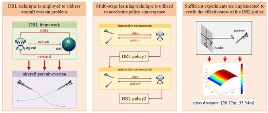
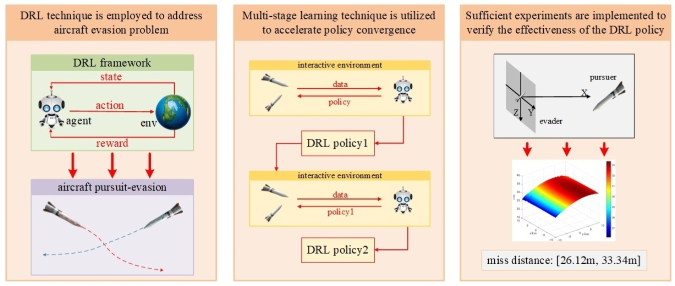
  • An MS-DDQN algorithm is proposed to improve the typical DQN algorithm to accelerate the convergence process and modify the quality of training data;
  • An adaptive iterative learning framework is implemented for high-speed aerial vehicle evasion problems;
  • Adequate comparative simulation experiments are implemented to verify the effectiveness and robustness of the proposed MS-DDQN algorithm.
The remainder of this paper is organized as follows: Section 2 presents the fundamental and problem formation. Section 3 introduces the MS-DDQN model and proposes the learning process to obtain the optimal evasion strategy. Section 4 presents the simulation experiments, and finally, Section 5 concludes this work.

2. Fundamental and Problem Formulation

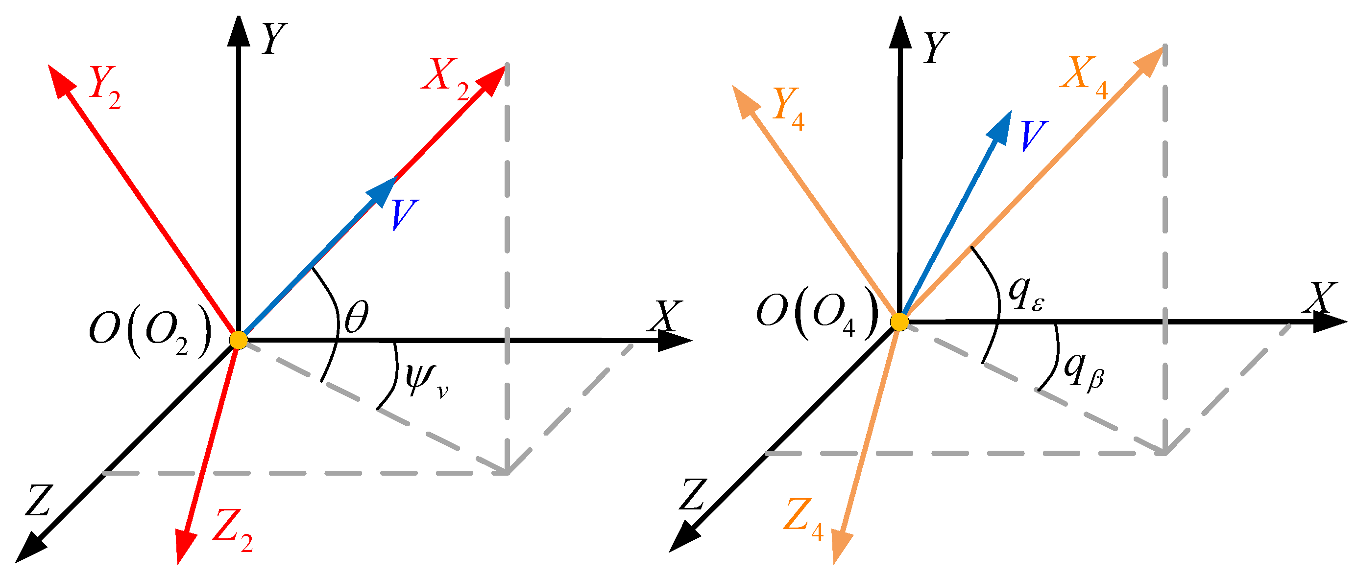
2.1. Aerial Vehicle Pursuit–Evasion Model

This section proposes the pursuit–evasion model of two vehicles to provide an interactive simulation environment for the problem.
It is a one-pursuer one-evader scenario where two agents are moving toward one another, whose projection distance in the X-axis of the velocity–turn–climb coordinate system is r 0 = 150   km . The pursuer uses a proportional navigation guidance (PNG) law to attack the evader with a maneuver period of T P = 15   ms and the maximum acceleration is a m a x P = 4.5   g , where g = 9.8   m / s 2 . The evader has four typical ignition pulse engines with a maneuver period of T E = 50   ms to avoid the pursuer’s attack with a maximum acceleration of a m a x E = 7.5   g . The orientation of the acceleration generated by the engines is perpendicular to the direction of the body. To make our testing scenario more challenging, we chose a larger velocity. The pursuer’s velocity was V P = 1.875   km / s , and the evader’s velocity was V E = 4.5   km / s . In this scenario, the evader is the agent that needs to be trained, while the pursuer is part of the simulation environment for the DRL problem described in this scenario. The agent learns the optimal evasion strategy by interacting with the pursuer to maximize the minimal miss, thoroughly discussed in Section 3.
The inertial reference frame, velocity–turn–climb coordinate frame, and line-of-sight (LOS) coordinate frame are denoted as O X Y Z ( S 0 ) , O 2 X 2 Y 2 Z 2 ( S 2 ) , and O 4 X 4 Y 4 Z 4 ( S 4 ) , respectively. For simplicity, the pursuer is denoted as P and the evader as E. Let θ i | i = P , E be the flight path angle and ψ v i | i = P , E the heading angle. q ϵ and q β are the horizontal and vertical LOS angles, and the horizontal and vertical LOS rotational rates are represented by q ˙ ϵ and q ˙ β , respectively. As presented in Equations (1) and  (2), C 2 0 and C 4 0 are the transformation matrices from S 2 to S 0 and from S 4 to S 0 , respectively.
C 2 0 = cos θ i cos ψ v i sin θ i sin ψ v i sin ψ v i sin θ i cos θ i 0 cos θ i sin ψ v i sin θ i sin ψ v i cos ψ v i i = P , E ,
C 4 0 = cos q ϵ cos q β sin q ϵ sin q β sin q β sin q ϵ cos q ϵ 0 cos q ϵ sin q β sin q ϵ sin q β cos q β .
Figure 1 Left illustrates the conversion relationship between S 0 and S 2 , where θ is the flight path angle and ψ v is the heading angle. Figure 1 Right depicts the relationship between S 0 and S 4 defined by the LOS angles q ϵ and q β .
Let X i = x i y i z i | i = P , E be the agent’s location in S 0 and let V 2 i = V i 0 0 | i = P , E be the vehicle’s velocity in S 2 . Then, we have:
V 0 i = C 2 0 V 2 i = v 0 x i v 0 y i v 0 z i | i = P , E ,
where V 0 i , i = P , E is the vehicle’s velocity in S 0 . The location’s derivative can be depicted as:
x ˙ i = V i cos θ i cos ψ v i | i = P , E y ˙ i = V i cos θ i | i = P , E z ˙ i = V i cos θ i sin ψ v i | i = P , E .
Let a 4 i = 0 a i y a i z | i = P , E be the aerial vehicle’s acceleration in S 4 ; then, we have:
a 0 i = C 4 0 a 4 i | i = P , E ,
where a 0 i | i = P , E is the vehicle’s acceleration in S 0 . V ˙ 0 i is also reformulated as:
v ˙ 0 x i = V i cos q ϵ cos q β | i = P , E v ˙ 0 y i = V i cos q ϵ | i = P , E v ˙ 0 z i = V i cos q ϵ sin q β | i = P , E .
Equations (7)–(10) are the formulas of q ϵ , q β , q ˙ ϵ , and q ˙ β in S 4 , respectively.
q ϵ = arctan r y r x 2 + r z 2 ,
q β = arctan r z r x ,
q ˙ ϵ = r x 2 + r z 2 r ˙ y r y r x r ˙ x + r z r ˙ z r x 2 + r y 2 + r z 2 r x 2 + r z 2 ,
q ˙ β = r z r ˙ x r x r ˙ z r x 2 + r z 2 ,
where r x = x E x P , r y = y E y P , r z = z E z P , r ˙ x = x ˙ E x ˙ P , r ˙ y = y ˙ E y ˙ P , and r ˙ z = z ˙ E z ˙ P .
According to the basic principle of PNG, the pursuer’s acceleration of a 4 P in S 4 is given by:
a 4 P = 0 N 4 y v q ˙ ϵ N 4 z v q ˙ β r = r x 2 + r y 2 + r z 2 v s . = r x r ˙ x + r y r ˙ y + r z r ˙ z r ,
where N 4 y = 4 and N 4 z = 5 are the PNG’s navigation ratios. Then, the aerial vehicle pursuit-evasion model can be defined by combining Equations (3)–(11)
X i = x i y i z i | i = P , E x ˙ i = V i cos θ i cos ψ v i | i = P , E y ˙ i = V i cos θ i | i = P , E z ˙ i = V i cos θ i sin ψ v i | i = P , E V 0 i = v 0 x i v 0 y i v 0 z i | i = P , E a 0 i = C 4 0 a 4 i | i = P , E a 4 P = 0 N 4 y v q ˙ ϵ N 4 z v q ˙ β a 4 E = 0 a 4 E y a 4 E z ,
where a 4 e y and a 4 e z are the evader’s accelerations in S 4 .

2.2. Value-Based Reinforcement Learning

An RL problem can be uniquely defined by a Markov decision process (MDP) [22] tuple S , P , R , γ , A , where S is the state space of the agent, P is the state transition probability matrix, R is the reward function, γ is the discount factor of the cumulative reward, and A is the action space. MDP is the fundamental framework of RL, where each episode starts with the initial condition and ends with the termination condition. When the agent takes action, it gets an immediate reward R t and transfers to another state s t + 1 . An RL problem intends to search for an optimal policy for a given MDP to maximize the cumulative reward G t , introduced in Equation (13), and the optimal policy π * is a distribution of an action space A for a fixed state s, introduced in Equation (14).
G t = k = 0 T γ k r t + k + 1 = r t + 1 + γ G t + 1 ,
π * a | s = P A t = a | S t = s .
In this aerial vehicle evasion problem, the state is the line-of-sight angles ( q ε and q β ) and the distance (r) of the two aerial vehicles, while the action is the operational status of the four pulse engines on or off. The designs of γ and R are implemented in Section 3.3, and the termination conditions of this problem are as follows:
  • The evader is successfully intercepted by the pursuer, which is called failure evasion;
  • The evader escapes from the attack of the pursuer successfully, which is called a successful evasion.
The RL algorithms comprise value-based [23], policy-based [24], and actor-critic [25]. For a value-based discrete time MDP (DT-MDP), to maximize the cumulative reward G t , the agent chooses an action according to the state-value function (Q-Function; Equation (15)) to iteratively update the policy until π converges to the optimal solution π * .
Q π s , a = E π G t | S t = s t , A t = a   = E π k = 0 T γ k r t + k + 1 | S t = s t , A t = a .
More specifically, a neural network is chosen as a value function approximator of Equation (15). In the optimal scenario, the agent chooses a greedy policy according to π * :
π * s = arg max a A Q π * s , a , ω ,
where ω is the parameter of the neural network.

3. MS-DDQN Algorithm Design

This section introduces the basic structure of the dueling DQN framework, proposes the MS-DDQN algorithm, and provides details on the learning process.

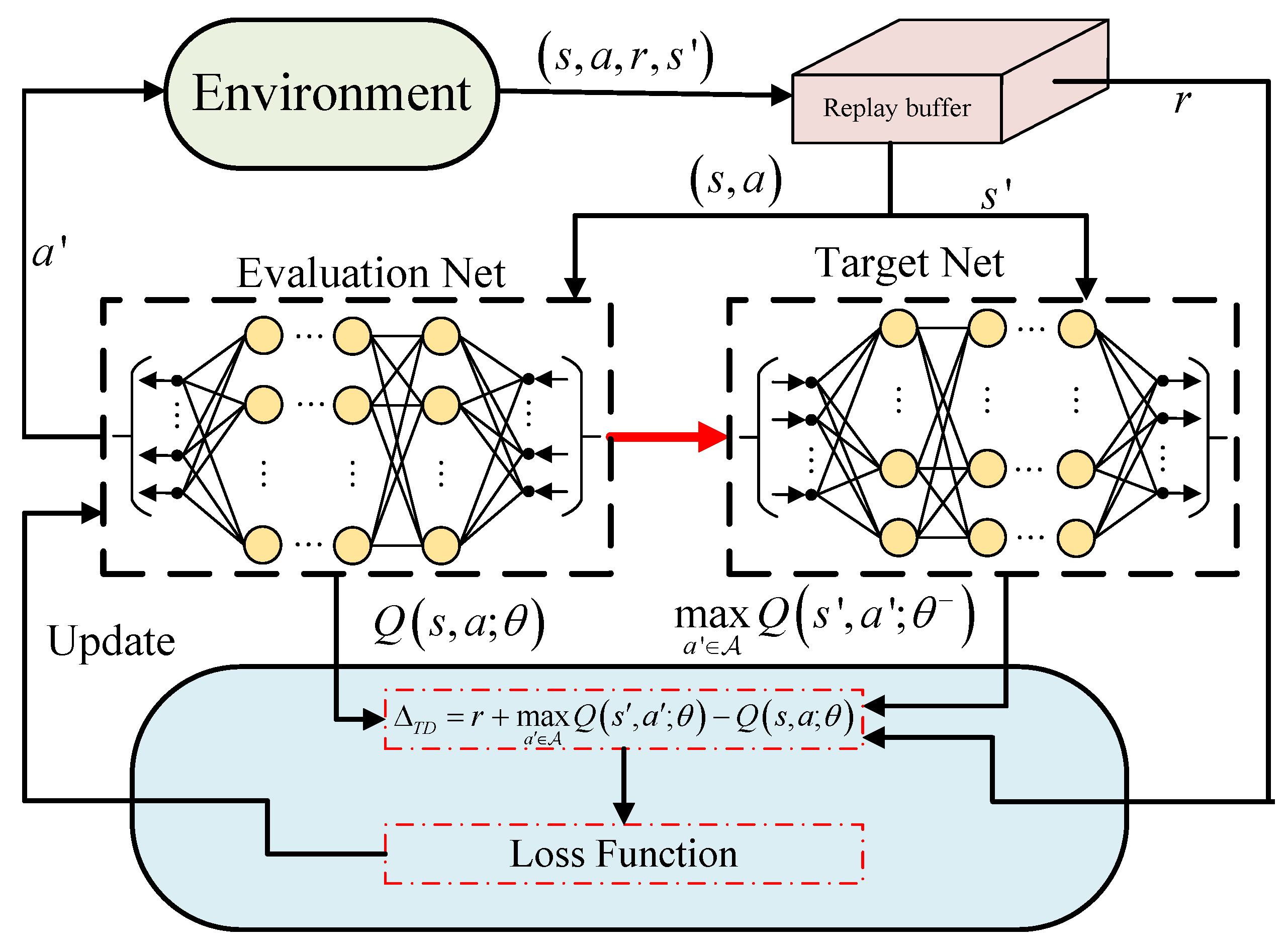
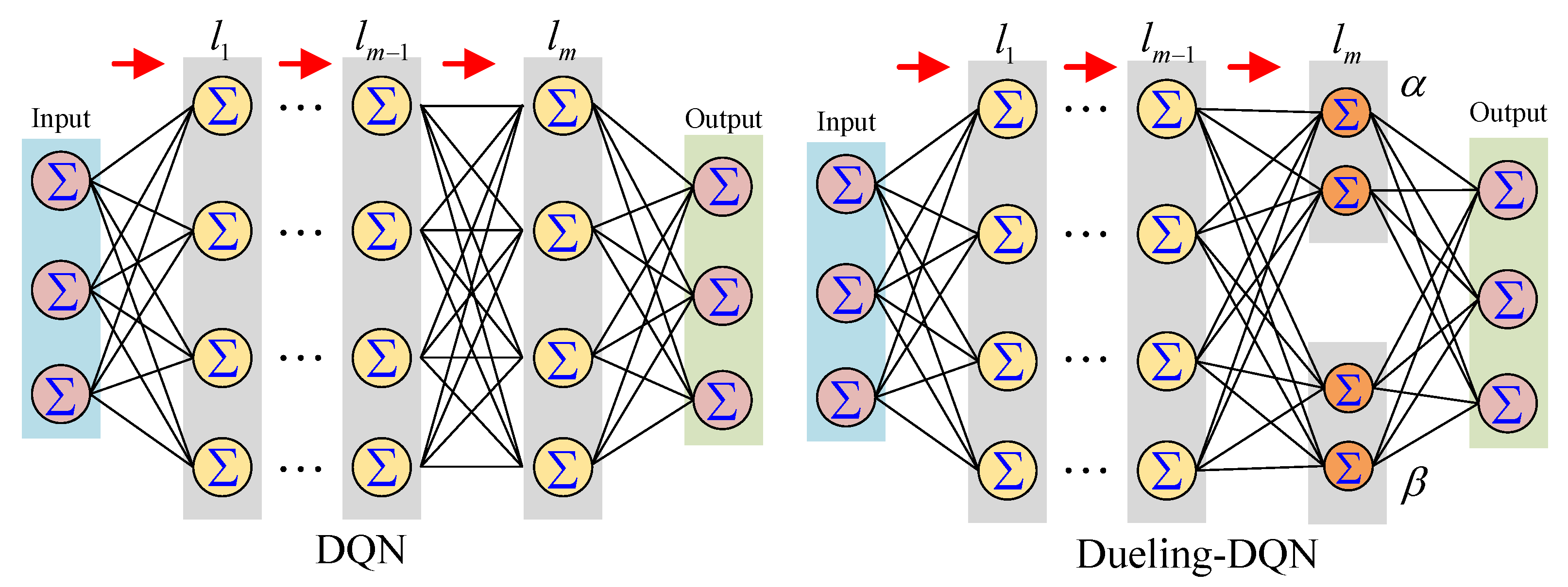
3.1. Dueling DQN Framework

The MS-DDQN framework is a multi-stage value-based DRL method, which improves the traditional DQN. The DQN establishes a direct connection between perception and the decision-making level of an autonomous system [26], as illustrated in Figure 2, where the replay memory collects data generated from the interaction between the agent (Evaluation Net) and the environment.
The sign of the convergence of the algorithm TD error converges to 0, and the TD error is calculated in the loss function module employing the formula Δ T D = r + max a A Q s , a ; θ Q s , a ; θ . The θ parameters in the evaluation net are updated by the loss function utilizing a suitable gradient descent algorithm. Moreover, the θ parameters in the target net are copied from θ every C step, where C is a constant. The learning process ends when Δ T D 0 .
However, DQN overfits the neural network approximator, overestimating the state’s value function. To overcome this drawback, Wang et al. [27] proposed a dueling network architecture that weakens the Q-network’s overestimation. Specifically, the dueling Q-network defines an advantage function to decouple the state-value function and the state-action-value function, as shown in Equation (17):
Q S , A , ω , α , β = V S , ω , α + A S , A , ω , β ,
where ω , α , and β are the parameters that need to be optimized. Specifically, α is the parameter of the value function V S , ω , α , β is the parameter of the advantage function A S , A , ω , β , and ω is the parameter that two functions have in common. Equation (17) is often written in the form of Equation (18) to reflect the identifiability of simulated physical experiments.
Q S , A , ω , α , β = V S , ω , α + A S , A , ω , β 1 A a A A S , a , ω , β .
Figure 3 illustrates the difference between DQN and dueling DQN. Both networks involve m hidden layers and the same input–output dimension. The last hidden layer in the bottom figure of Figure 3 is divided into two parts: V S , ω , α and A S , A , ω , β , while the dueling DQN output is the sum of V · and A · .
Figure 4 illustrates the complete learning process. In Figure 4, O D E is the model state-solving module for state update, C F is the coordinate transformation module, and P G is the proportional guide law module that generates the acceleration command for the pursuer. The “policy learning” module in Figure 4 is the RL learning process shown in Figure 2. The “RL maneuver” is the training result of “policy learning”, which is used to generate acceleration commands for the evader. The entire framework is a recurrent process and terminates when the evader can get rid of the pursuer’s attack.

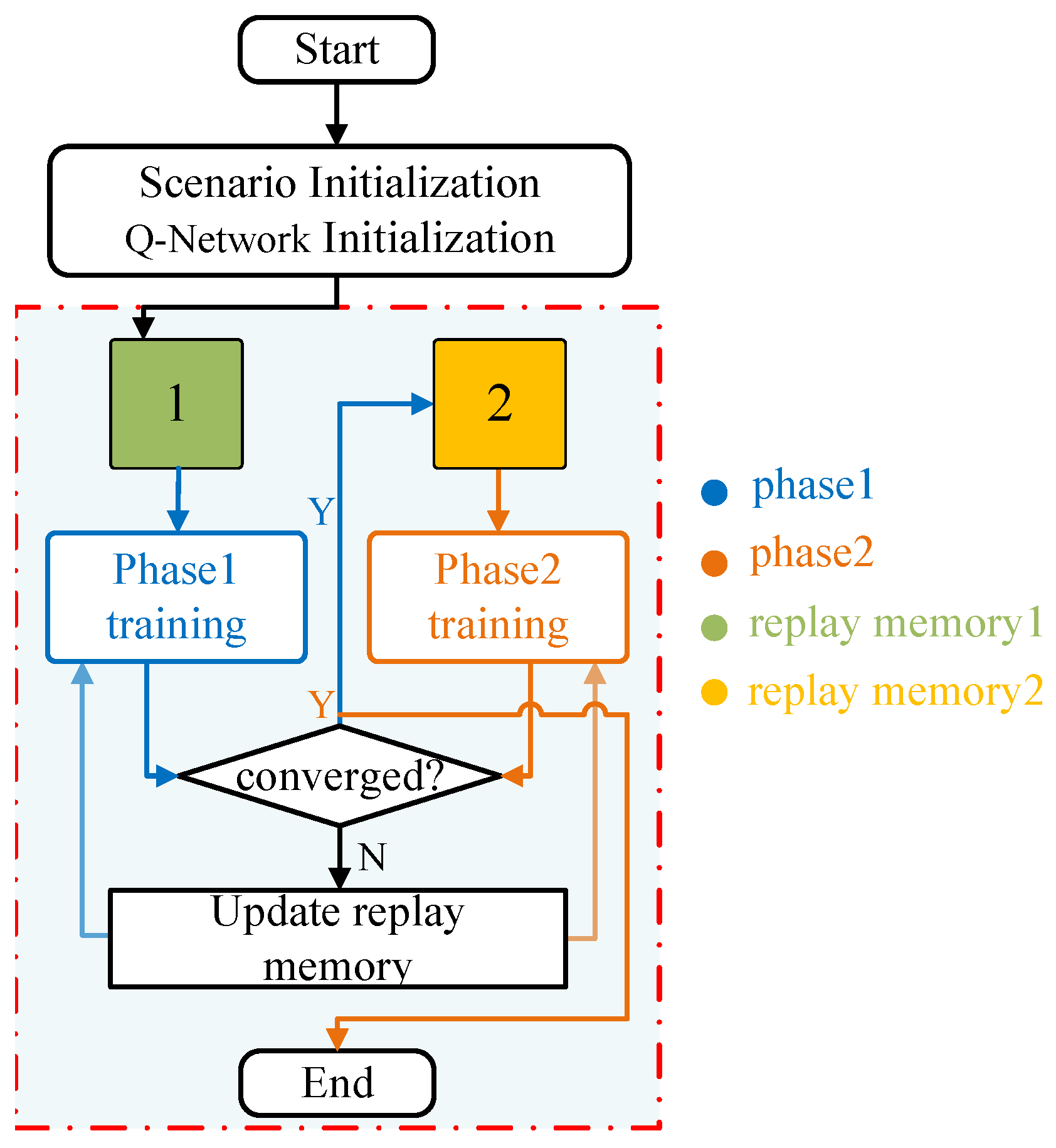
3.2. Multi-Stage Learning

DRL methods iteratively learn the optimal policy through interacting with the environment. Nonetheless, it is almost impossible for an agent to collect adequate high-quality sampling data with an initial stochastic policy when the state space is vast. Therefore, a multi-stage learning scheme is proposed to speed up the agent’s learning process by inserting several sub-mission nodes during the entire learning process to guide the agent step-by-step in reasonably learning the optimal policy. This idea is inspired by humans’ solutions to complex problems, as we typically decompose a considerable problem into several smaller ones that are serially connected. The solution of a sub-task is the initial condition of the next one.
The entire task is divided into two sub-tasks for the evasion problem examined in this paper. In the first training phase, the agent learns an applicable policy π t e m p with a certain stochastic exploration probability. π t e m p is a relatively ideal initial condition for second-stage training, although not the optimal policy with a high probability. The objective of second-stage training is to find an optimal policy π that maximizes the miss based on π t e m p by using the adequate high-quality data generated by the initial acceptable policy in the first stage of learning. Algorithm 1 presents the pseudo-code of this multi-stage training framework.
Algorithm 1 A multi-stage training framework with N sub-missions.
  •  Input: N, Reward function for each phase f i , i = 1 , 2 , , N , an initial policy π 0 .
1:
Output: The optimal policy π
2:
Environment initialization: i = 0 , empty the replay memory.
3:
while i < N do
4:
    Initialize the neural network.
5:
    Fill the replay memory with sampling data generated by policy π i , ε i . ( ε i is a certain initial exploration probability for the i t h  phase.)
6:
    while  π i is not converged do
7:
        Network training in Dueling-DQN framework with reward function f i .
8:
        Update π i and replay memory.
9:
    Save π i , i + = 1 .
10:
return  π

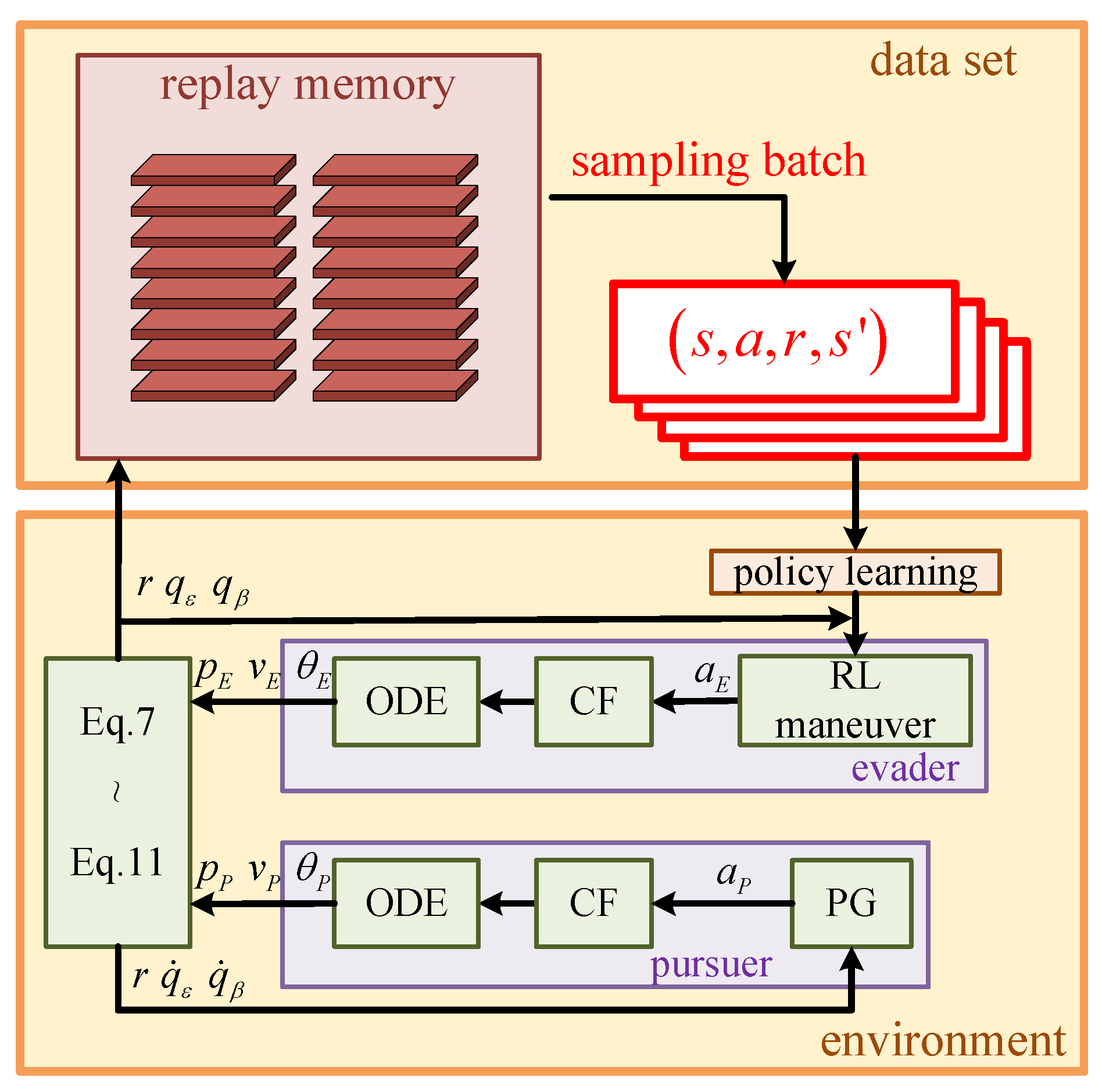
3.3. Complete Learning Framework

The MS-DDQN method has four key elements: State space, action space, reward functions for each training phase, and the neural network structure. The choice of state space predominantly affects the quality of the final policy. In the vehicle evasion scenario, the distance, and LOS angles ( q ϵ and q β ) are the three crucial factors, and Equation (19) denotes the agent’s state:
s = r , q ϵ , q β ,
where r is the distance between the two vehicles and q ϵ and q β are the LOS angles. The evader in this scenario maneuvers with four ignition pulse engines, hence the evader has nine maneuvering types (Table 1); the action’s dimension is one, with the agent selecting one of the nine actions according to the policy each time.
The three elements in each action in Table 1 are the evader’s acceleration in X, Y, and Z. ‘ + m a x ’ means the acceleration reaches the maximum value, and ‘ m a x ’ is the minimum value (reverse maximum).
The choice of the reward function is another decisive factor in the training process. It should be a continuous function of the state, with the reward function of the first and second training phases given in Equations (20) and (21), respectively.
r 1 = k 1 max q ϵ , q β 2 r 2 = 10000                       i f   e v a s i o n   s u c c e e d e d 0                             i f   e v a s i o n   f a i l e d r = r 1 + r 2 k 1 = 200 tan 0.1047 t 1.5184   i f   a c t i o n = 0 , 1 , 2 , 3 , 4 50 tan 0.1047 t 1.5184       i f   a c t i o n = 5 , 6 , 7 , 8 ,
r 1 = k 1 max q ϵ , q β 2 r 2 = 1000 r 2                     i f   e v a s i o n   s u c c e e d e d 0                             i f   e v a s i o n   f a i l e d r = r 1 + r 2 k 1 = 200 tan 0.1047 t 1.5184   i f   a c t i o n = 0 , 1 , 2 , 3 , 4 50 tan 0.1047 t 1.5184       i f   a c t i o n = 5 , 6 , 7 , 8 .
In Equations (20) and (21), the reward function is divided into two parts: The reward for the approaching process r 1 and the reward for the episode termination r 2 . k 1 is the coefficient of r 1 , which is originally designed to affect the sensitivity of r 1 to the LOS angles and increases with time. The design of k 1 formation guides the agent to consume the remaining fuel at the end of the escape to increase its line of sight with the pursuer. The introduction of the tangent function ensures that the reward is more sensitive to the agent’s action as time increases. The purpose of r 1 is to maximize one of the LOS angles, considering that the Y-direction is symmetrical to the Z-direction and r 2 is different in the two training phases. Therefore, the aim is to find, for the aerial vehicle, an acceptable policy in the first training phase and to maximize the miss in the second training phase.
Additionally, r 1 still exists in the second learning stage to avoid sparse rewards in RL. A sparse reward problem, i.e., the agent can get a nonzero reward if, and only if, it completes an episode of exploration, means that the agent does not have adequate data to modify its action [28]. It is hard for RL algorithms to converge when dealing with sparse reward problems. Therefore, both r 1 and r 2 are added to the reward function to ensure the adequacy of the training data.
The MS-DDQN estimates the policy’s value function through a Q-network. Table 2 presents the neural network structure, where 3 V and 3 A are the value and advantage parts of the Q function, respectively, and R e L u ( ) is the activation function of the neural network.
Figure 5 illustrates the flow diagram of the training process. First, the flow chart presents the left channel to start first-phase training. Then, it continues to perform the second training phase after an acceptable policy is obtained, which is the initial policy of the second phase. The capacities of the two-training phase are hyper-parameters that need to be tuned manually. Finally, the algorithm stops when the target network converges. Furthermore, this paper adopted the network-retraining technique proposed in [29,30,31] to strengthen the network training quality.
The network training consists of procedures, initialization, and training. The data input into the replay memories during the initialization part are generated by the current temporary optimal policy with certain exploration probabilities ϵ 1 = 0.2 and ϵ 2 = 0.2 . For the first stage of the training part, the optimal temporary policy is stochastic. In contrast, the second stage of the training part takes the policy generated by the first stage as the initial temporary optimal policy. Figure 6 depicts the relationship between the episode and exploration probability during the training process. The functional relationship between the exploration probability and episode is designed as an exponential function to make the agent’s exploration more adequate. The mathematical function of each segment in Figure 6 is presented at the right top of the figure. Episodes 0–1499 belong to the first training of the first phase, while episodes 1500–2099 are the second training of the first phase, and episodes 2100–2999 belong to the training in the second phase.
Table 3 lists the hyper-parameters of MS-DDQN, where γ denotes the discount factor of RL, ϵ 0 is the initial exploration probability, α is the learning rate of the Q-network, M is the capacity of the replay memory, and B a t c h   S i z e is the number of samples extracted each time during the Q-network learning.

4. Simulation Experiments

This section evaluates the evasion performance employing the strategy generated by MS-DDQN. For clarity, we rearranged the parameters presented in Section 2.1 into Table 4.
Here, r 0 is the initial relative distance in the LOS coordinate frame ( S 4 ) of the two vehicles, T i | i = P , E is the maneuver cycle of the vehicle, a m a x i | i = P , E is the maximum acceleration of the vehicle in the LOS coordinate frame ( S 4 ), and V i | i = P , E is the velocity of the vehicle in LOS coordinate frame ( S 4 ).
Figure 7 represents the relationship between the cumulative reward and episode in both multi- and single-phase training. Simultaneously, the curves verify the effectiveness of the multi-phase training. Figure 7 highlights that the average reward increased significantly as the episode increased in phase1 training. However, the average reward decreased slightly in episodes 1500–2100 due to the increase in ϵ (see Figure 6), which means the agent explored the environment stochastically with a higher probability. Based on phase1, the average reward of phase2 was substantially higher than that of phase1, indicating a successful evasion and the effectiveness of the two-stage training technique implemented in the training process. Finally, the evader achieved a high-quality policy after 2700 training episodes. However, without multi-phase training, the single-phase training process maintained a low-level cumulative reward throughout the entire training process.
Comparative simulation experiments were designed on the miss distances of the evader using various maneuvers. Figure 8 and Figure 9 illustrate the simulation results when the evader implemented a random maneuvering policy and a square wave maneuver policy, respectively.
The misses were 0.20   m and 0.26   m , respectively, and the simulation time is 24.057   s . The results indicate that the evader could not use traditional maneuvers to avoid the pursuer’s attack. Figure 10, Figure 11 and Figure 12 present the simulation results when the evader applied a neural network maneuver strategy generated by MS-DDQN. The scenarios involved nine relative locations with an initial flight path angle θ and a heading angle of 0. We conclude that the miss is much more significant than the traditional maneuver.
Figure 10 presents the evasion process when the evader implemented the policy generated by MS-DDQN with the initial relative positions 20   km , 20   km , 20   km , 0   km , and 20   km , 20   km in the initial inertial coordinate system. The results indicate that the slightest miss of the three scenarios was 18.4174   m , satisfying the problem requirement. Additionally, the figures for t i m e a y and t i m e a z illustrate that the evader tended to consume all of the remaining fuel at the end of the interception to increase its line of sight with the pursuer, which can be found in the figure for t i m e a y . Allocating all fuel in the Y-direction, the output of the Z-direction remained zero throughout the process due to the limited fuel. Figure 11 and Figure 12 indicate the results from the same law as Figure 10.
To further demonstrate the feasibility of the MS-DDQN maneuver, more simulation experiments with different relative initial positions, flight path angles θ , and heading angles Ψ v are presented. Table 5, Table 6, Table 7, Table 8 and Table 9 present the simulation results with an initial θ of 10°, 5°, 0°, 5 ° , and 10 ° , respectively.
Table 5, Table 6, Table 7, Table 8 and Table 9 illustrate that the slightest miss of these 225 scenarios was 6.58   m , satisfying the evasion problem requirement.
The simulation experiments indicate that the evading policy generated by MS-DDQN can avoid the pursuer’s attack in a large domain. For clarity, we also conducted a generic simulation experiment by uniformly sampling 10,000 points in a range of 20 × 20   km with initial θ = 5 ° and Ψ v = 5 ° (Figure 13).
This figure illustrates a successful evasion of the evader where the missing range is 26.12   m , 33.34   m .

5. Conclusions

This paper proposed an MS-DDQN algorithm to address the problem of high-speed aircraft evading. The evader was treated as the agent for DRL, and the optimal policy was generated through iteratively interacting with the simulation environment by the MS-DDQN framework. Moreover, the proposed two-stage learning method significantly improved the data quality and sped up the training process. As a model-free RL algorithm, MS-DDQN is an adaptive value-based DRL framework that does not require the vehicle’s mathematical model.
The effectiveness and robustness of this method were verified through various simulation experiments, illustrating a successful evasion in a large domain when utilizing the policy generated by MS-DDQN. Future research on autonomous decisions for evasion will combine policy-based DRL methods and multi-vehicle autonomous decision-making systems.

Author Contributions

Conceptualization, Y.Y.; methodology, Y.Y. and T.H.; software, Y.Y.; validation, Y.Y. and T.H.; formal analysis, Y.Y. and X.W.; investigation, Y.Y. and X.H.; resources, Y.Y. and T.H.; data curation, Y.Y. and T.H.; writing—original draft preparation, Y.Y.; writing—review and editing, Y.Y., T.H., X.W. and C.-Y.W.; visualization, Y.Y.; supervision, C.-Y.W. and X.H.; project administration, Y.Y. and X.H. All authors have read and agreed to the published version of the manuscript.

Funding

This research received no external funding.

Institutional Review Board Statement

Not applicable.

Informed Consent Statement

Not applicable.

Data Availability Statement

Not applicable.

Conflicts of Interest

The authors declare that they have no conflict of interest or personal relationships that could have appeared to influence the work reported in this paper.

References

  1. Zeng, X.; Yang, L.; Zhu, Y.; Yang, F. Comparison of Two Optimal Guidance Methods for the Long-Distance Orbital Pursuit-Evasion Game. IEEE Trans. Aerosp. Electron. Syst. 2021, 57, 521–539. [Google Scholar] [CrossRef]
  2. Lee, J.; Ryoo, C. Impact Angle Control Law with Sinusoidal Evasive Maneuver for Survivability Enhancement. Int. J. Aeronaut. Space Sci. 2018, 19, 433–442. [Google Scholar] [CrossRef]
  3. Si, Y.; Song, S. Three-dimensional adaptive finite-time guidance law for intercepting maneuvering targets. Chin. J. Aeronaut. 2017, 30, 1985–2003. [Google Scholar] [CrossRef]
  4. Song, J.; Song, S. Three-dimensional guidance law based on adaptive integral sliding mode control. Chin. J. Aeronaut. 2016, 29, 202–214. [Google Scholar] [CrossRef] [Green Version]
  5. He, L.; Yan, X. Adaptive terminal guidance law for spiral-diving maneuver based on virtual sliding targets. J. Guid. Control Dynam. 2018, 41, 1591–1601. [Google Scholar] [CrossRef]
  6. Xu, X.; Cai, Y. Design and numerical simulation of a differential game guidance law. In Proceedings of the 2016 IEEE International Conference on Information and Automation (ICIA), Ningbo, China, 31 July–4 August 2016; pp. 314–318. [Google Scholar]
  7. Alias, I.; Ibragimov, G.; Rakhmanov, A. Evasion differential game of infinitely many evaders from infinitely many pursuers in Hilbert space. Dyn. Games Appl. 2017, 7, 347–359. [Google Scholar] [CrossRef]
  8. Liang, L.; Deng, F.; Peng, Z.; Li, X.; Zha, W. A differential game for cooperative target defense. Automatica 2019, 102, 58–71. [Google Scholar] [CrossRef]
  9. Ibragimov, G.; Ferrara, M.; Kuchkarov, A.; Pansera, B.A. Simple motion evasion differential game of many pursuers and evaders with integral constraints. Dyn. Games Appl. 2018, 8, 352–378. [Google Scholar] [CrossRef]
  10. Rilwan, J.; Kumam, P.; Badakaya, A.J.; Ahmed, I. A Modified Dynamic Equation of Evasion Differential Game Problem in a Hilbert space. Thai J. Math. 2020, 18, 199–211. [Google Scholar]
  11. Jagat, A.; Sinclair, A.J. Nonlinear Control for Spacecraft Pursuit-Evasion Game Using the State-Dependent Riccati Equation Method. IEEE Trans. Aerosp. Electron. Syst. 2017, 53, 3032–3042. [Google Scholar] [CrossRef]
  12. Asadi, M.M.; Gianoli, L.G.; Saussie, D. Optimal Vehicle-Target Assignment: A Swarm of Pursuers to Intercept Maneuvering Evaders based on Ideal Proportional Navigation. IEEE Trans. Aerosp. Electron. Syst. 2021, 58, 1316–1332. [Google Scholar] [CrossRef]
  13. Waxenegger-Wilfing, G.; Dresia, K.; Deeken, J.; Oschwald, M. A Reinforcement Learning Approach for Transient Control of Liquid Rocket Engines. IEEE Trans. Aerosp. Electron. Syst. 2021, 57, 2938–2952. [Google Scholar] [CrossRef]
  14. Silver, D.; Huang, A.; Maddison, C.; Guez, A.; Sifre, L.; van den Driessche, G.; Schrittwieser, J.; Antonoglou, L.; Panneershelvam, V.; Lanctot, M.; et al. Mastering the game of Go with deep neural networks and tree search. Nature 2016, 529, 484–489. [Google Scholar] [CrossRef]
  15. Sun, J.; Liu, C.; Ye, Q. Robust differential game guidance laws design for uncertain interceptor-target engagement via adaptive dynamic programming. Int. J. Control 2016, 90, 990–1004. [Google Scholar] [CrossRef]
  16. Gaudet, B.; Furfaro, R.; Linares, R. Reinforcement learning for angle-only intercept guidance of maneuvering targets. Aerosp. Sci. Technol. 2020, 99, 105746. [Google Scholar] [CrossRef] [Green Version]
  17. Zhu, J.; Zou, W.; Zhu, Z. Learning Evasion Strategy in Pursuit-Evasion by Deep Q-network. In Proceedings of the 2018 24th International Conference on Pattern Recognition (ICPR), Beijing, China, 20–24 August 2018; pp. 67–72. [Google Scholar]
  18. Li, C.; Deng, B.; Zhang, T. Terminal guidance law of small anti-ship missile based on DDPG. In Proceedings of the International Conference on Image, Video Processing and Artificial Intelligence, Shanghai, China, 21 August 2020; Volume 11584. [Google Scholar]
  19. Shalumov, V. Cooperative online Guide-Launch-Guide policy in a target-missile-defender engagement using deep reinforcement learning. Aerosp. Sci. Technol. 2020, 104, 105996. [Google Scholar] [CrossRef]
  20. Souza, C.; Nwebury, R.; Cosgun, A.; Castillo, P.; Vidolov, B.; Kulić, D. Decentralized Multi-Agent Pursuit Using Deep Reinforcement Learning. IEEE Robot. Autom. Let. 2021, 6, 4552–4559. [Google Scholar] [CrossRef]
  21. Tipaldi, M.; Iervoline, R.; Massenio, P.R. Reinforcement learning in spacecraft control applications: Advances, prospects, and challenges. Annu. Rev. Control 2022, in press. [CrossRef]
  22. Selvi, E.; Buehrer, R.M.; Martone, A.; Sherbondy, K. Reinforcement Learning for Adaptable Bandwidth Tracking Radars. IEEE Trans. Aerosp. Electron. Syst. 2020, 56, 3904–3921. [Google Scholar] [CrossRef]
  23. Ahmed, A.M.; Ahmad, A.A.; Fortunati, S.; Sezgin, A.; Greco, M.S.; Gini, F. A Reinforcement Learning Based Approach for Multitarget Detection in Massive MIMO Radar. IEEE Trans. Aerosp. Electron. Syst. 2021, 57, 2622–2636. [Google Scholar] [CrossRef]
  24. Hu, Q.; Yang, H.; Dong, H.; Zhao, X. Learning-Based 6-DOF Control for Autonomous Proximity Operations Under Motion Constraints. IEEE Trans. Aerosp. Electron. Syst. 2021, 57, 4097–4109. [Google Scholar] [CrossRef]
  25. Elhaki, O.; Shojaei, K. A novel model-free robust saturated reinforcement learning-based controller for quadrotors guaranteeing prescribed transient and steady state performance. Aerosp. Sci. Technol. 2021, 119, 107128. [Google Scholar] [CrossRef]
  26. Volodymyr, M.; Koray, K.; David, S.; Rusu, A.A.; Veness, J.; Bellemare, M.G.; Graves, A.; Riedmiller, M.; Fidjeland, A.K.; Ostrovski, G.; et al. Human-level control through deep reinforcement learning. Nature 2015, 518, 529–533. [Google Scholar]
  27. Wang, Z.; Schaul, T.; Hessel, M.; Hasselt, H.; Lanctot, M.; Freitas, N. Dueling network architectures for deep reinforcement learning. In Proceedings of the International Conference on Machine Learning, San Francisco, CA, USA, 14 August 2016; Volume 48, pp. 1995–2003. [Google Scholar]
  28. Wang, C.; Wang, J.; Wang, J.; Zhang, X. Deep-Reinforcement-Learning-Based Autonomous UAV Navigation with Sparse Rewards. IEEE Internet Things J. 2020, 7, 6180–6190. [Google Scholar] [CrossRef]
  29. Huang, T.; Liang, Y.; Ban, X.; Zhang, J.; Huang, X. The Control of Magnetic Levitation System Based on Improved Q-network. In Proceedings of the Symposium Series on Computational Intelligence, Xiamen, China, 6–9 December 2019; pp. 191–197. [Google Scholar]
  30. Fan, J.; Wang, Z.; Xie, Y.; Yang, Z. A Theoretical Analysis of Deep Q-Learning. In Proceedings of the Learning for Dynamics and Control, PMLR, Online, 11–12 June 2020; pp. 486–489. [Google Scholar]
  31. Razzaghi, P.; Khatib, E.A.; Bakhtiari, S.; Hurmuzlu, Y. Real time control of tethered satellite systems to de-orbit space debris. Aerosp. Sci. Technol. 2021, 109, 106379. [Google Scholar] [CrossRef]
Figure 1. Conversion relationship between S 0 , S 2 , and S 4 (Left: S 0 and S 2 . Right: S 0 and S 4 ). V is the velocity vector of the aircraft, θ is the flight path angle, ψ v is the heading angle, and q ϵ and q β are the LOS angles.
Aerospace 09 00673 g001
Figure 2. Schematic diagram of DQN.
Aerospace 09 00673 g002
Figure 3. Difference between the networks in DQN (left) and dueling DQN (right).
Aerospace 09 00673 g003
Figure 4. Complete learning framework.
Aerospace 09 00673 g004
Figure 5. Flow diagram of the MS-DDQN training process.
Aerospace 09 00673 g005
Figure 6. Relationship between episode n and exploration probability ϵ .
Aerospace 09 00673 g006
Figure 7. Comparative cumulative rewards of single- and multi-phase training.
Aerospace 09 00673 g007
Figure 8. Evader employing a random maneuver.
Aerospace 09 00673 g008
Figure 9. Evader employing a square maneuver.
Aerospace 09 00673 g009
Figure 10. Evader utilizing MS-DDQN maneuvers with the three different initial relative positions 20   km , 20   km , 20   km , 0   km , and 20   km , 20   km in the initial inertial coordinate system.
Aerospace 09 00673 g010
Figure 11. Evader utilizing MS-DDQN maneuvers with the three different initial relative positions 0   km , 20   km , 0   km , 0   km , and 20   km , 20   km in the initial inertial coordinate system.
Aerospace 09 00673 g011
Figure 12. Evader utilizing MS-DDQN maneuvers with the three different initial relative positions 20   km , 20   km , 20   km , 0   km , and 20   km , 20   km in the initial inertial coordinate system.
Aerospace 09 00673 g012
Figure 13. The curved surface of the miss distance and 10,000 different initial positions.
Aerospace 09 00673 g013
Table 1. Action space of the evader.
ActionAccelerationActionAccelerationActionAcceleration
0 0 0 0 3 0 0 + m a x 6 0 + m a x m a x
1 0 + m a x 0 4 0 0 m a x 7 0 m a x + m a x
2 0 m a x 0 5 0 + m a x + m a x 8 0 m a x m a x
Table 2. Structure of the neural network.
LayerInputOutputActivation Function
1320 R e L u ( )
22020
3V209
3A209
Table 3. Some hyper-parameters of MS-DDQN.
PhasePhase1-a Phase1-b Phase2
Parameter
γ 0.90.90.9
ϵ 0 0.90.90.9
α 0.010.010.01
M500050002000
B a t c h   S i z e 646464
Table 4. Parameters of the simulation scenario.
ParameterValueParameterValue
r 0 150   km g 9.8   m / s 2
T P 15   ms T E 50   ms
a m a x P 4.5   g a m a x E 7.5   g
V P 1.875   km / s V E 4.5   km / s
Table 5. Miss distance (m) with initial flight path angle θ = 10 ° .
Initial Relative
Distance (km)
Heading Angle Ψ v ( ° )
1050 5 10
20 , 20 19.8123.2525.1725.3625.45
20 , 0 23.8725.4125.6125.4324.21
20 , 20 25.6925.5324.9023.1218.80
0 , 20 24.1128.9729.9030.5030.69
0 , 0 30.2930.7130.7530.4829.71
0 , 20 30.9330.4929.7628.3223.92
20 , 20 13.719.7913.1513.7914.19
20 , 0 13.0813.8213.8213.512.50
20 , 20 14.3813.7112.569.796.67
Table 6. Miss distance (m) with initial flight path angle ( θ = 5 ° ).
Initial Relative
Distance (km)
Heading Angle Ψ v ( ° )
1050 5 10
20 , 20 20.1723.3025.6326.2126.13
20 , 0 24.6426.0226.2525.5624.02
20 , 20 25.8325.9825.2623.6019.21
0 , 20 28.9331.2531.9332.2132.42
0 , 0 32.4432.5632.4432.2231.72
0 , 20 32.6732.2231.6430.4928.12
20 , 20 14.1417.3916.9317.3617.90
20 , 0 17.9717.3417.1817.2016.87
20 , 20 17.9917.2116.6915.1813.66
Table 7. Miss distance (m) with initial flight path angle θ = 0 ° .
Initial Relative
Distance (km)
Heading Angle Ψ v °
1050 5 10
20 , 20 16.6122.1225.1925.4725.37
20 , 0 23.8225.1425.6325.3623.65
20 , 20 25.5925.7224.6822.1217.41
0 , 20 30.4532.1032.8033.0133.24
0 , 0 33.3333.3933.2333.0732.54
0 , 20 33.4833.0232.5331.2229.00
20 , 20 16.6919.1218.5719.0619.64
20 , 0 19.2219.1818.8118.8319.49
20 , 20 19.6818.9618.4218.0718.27
Table 8. Miss distance (m) with initial flight path angle θ = 5 ° .
Initial Relative
Distance (km)
Heading Angle Ψ v °
1050 5 10
20 , 20 11.1419.9223.1624.2124.17
20 , 0 21.3123.4323.9823.6921.08
20 , 20 23.9124.2422.8419.0710.31
0 , 20 29.1132.2732.8533.1233.36
0 , 0 33.2533.4933.3533.1532.52
0 , 20 33.5533.1232.5931.5629.19
20 , 20 18.5519.6519.7319.8520.47
20 , 0 20.6819.6819.5219.7019.96
20 , 20 20.4519.7719.4718.4818.74
Table 9. Miss distance (m) with initial flight path angle θ = 10 ° .
Initial Relative
Distance (km)
Heading Angle Ψ v °
1050 5 10
20 , 20 8.7015.9820.8822.2122.31
20 , 0 20.5021.6022.1221.5118.47
20 , 20 22.5122.2220.2215.946.58
0 , 20 26.7230.8331.9232.3432.54
0 , 0 32.1532.5332.5932.3431.37
0 , 20 32.7932.3231.6129.9725.76
20 , 20 19.8919.7919.6820.1520.72
20 , 0 20.6920.1519.8119.9020.54
20 , 20 20.7220.1019.5419.4617.85
Publisher’s Note: MDPI stays neutral with regard to jurisdictional claims in published maps and institutional affiliations.

