
Key Parameters of a Design for a Novel Reflux Subsonic Low-Density Dust Wind Tunnel


Abstract
1. Introduction
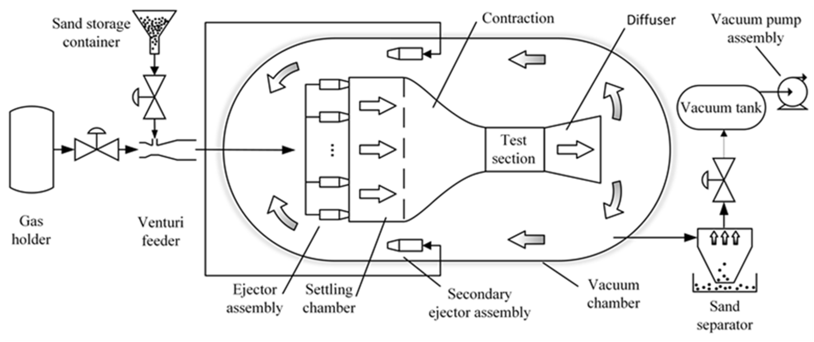
2. System Design
3. Detailed Parameters Discussion
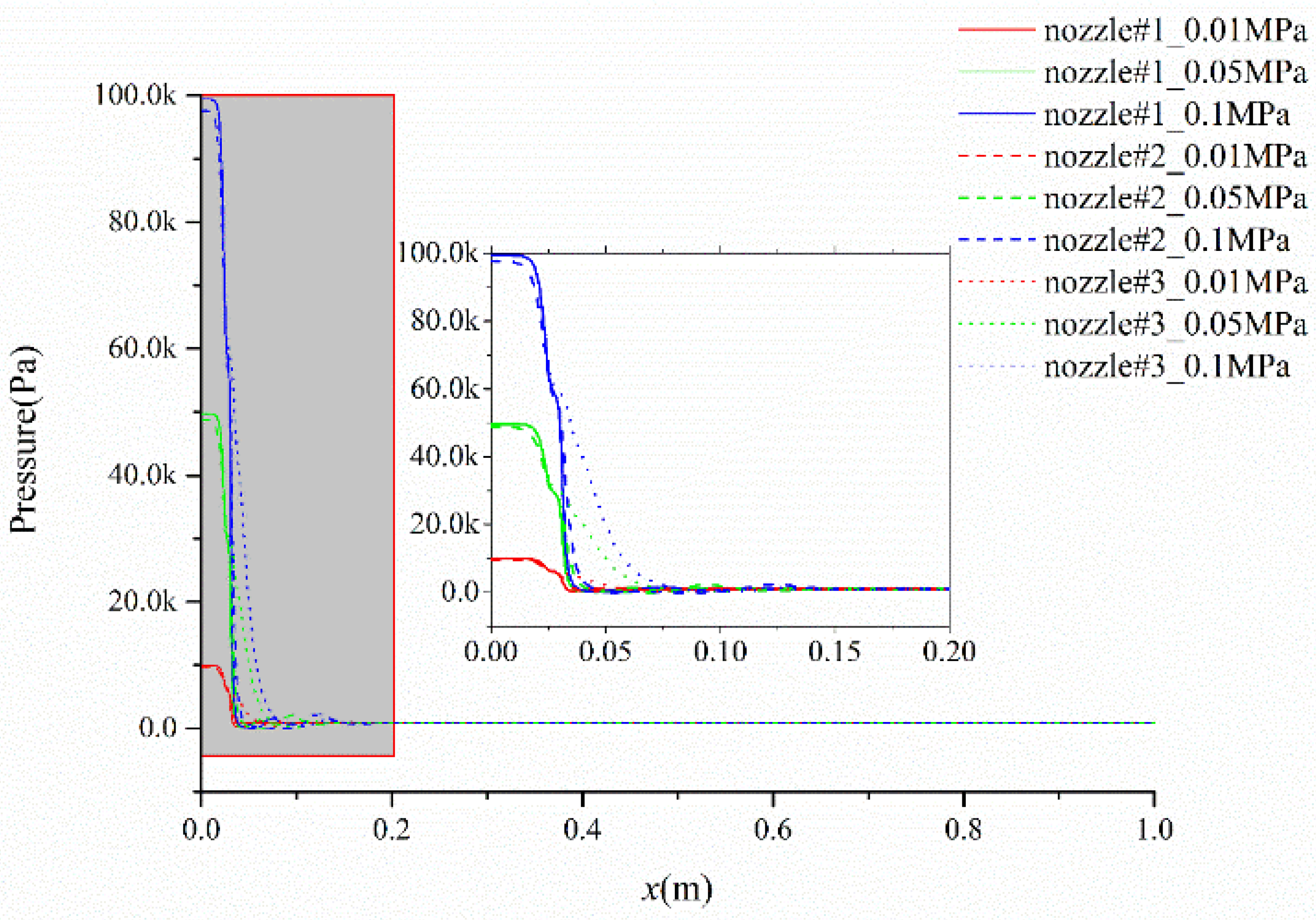
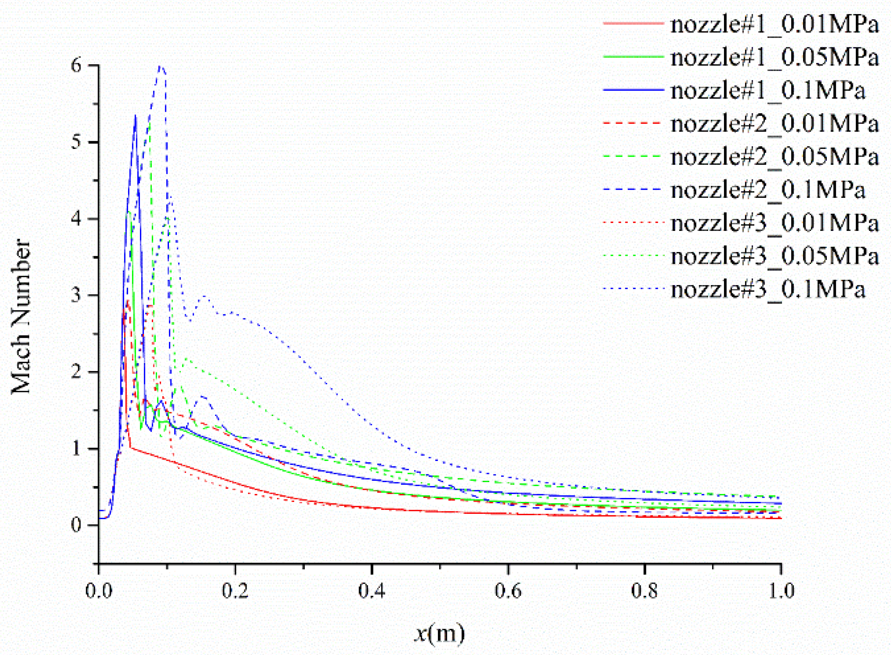
3.1. Nozzle Parameters
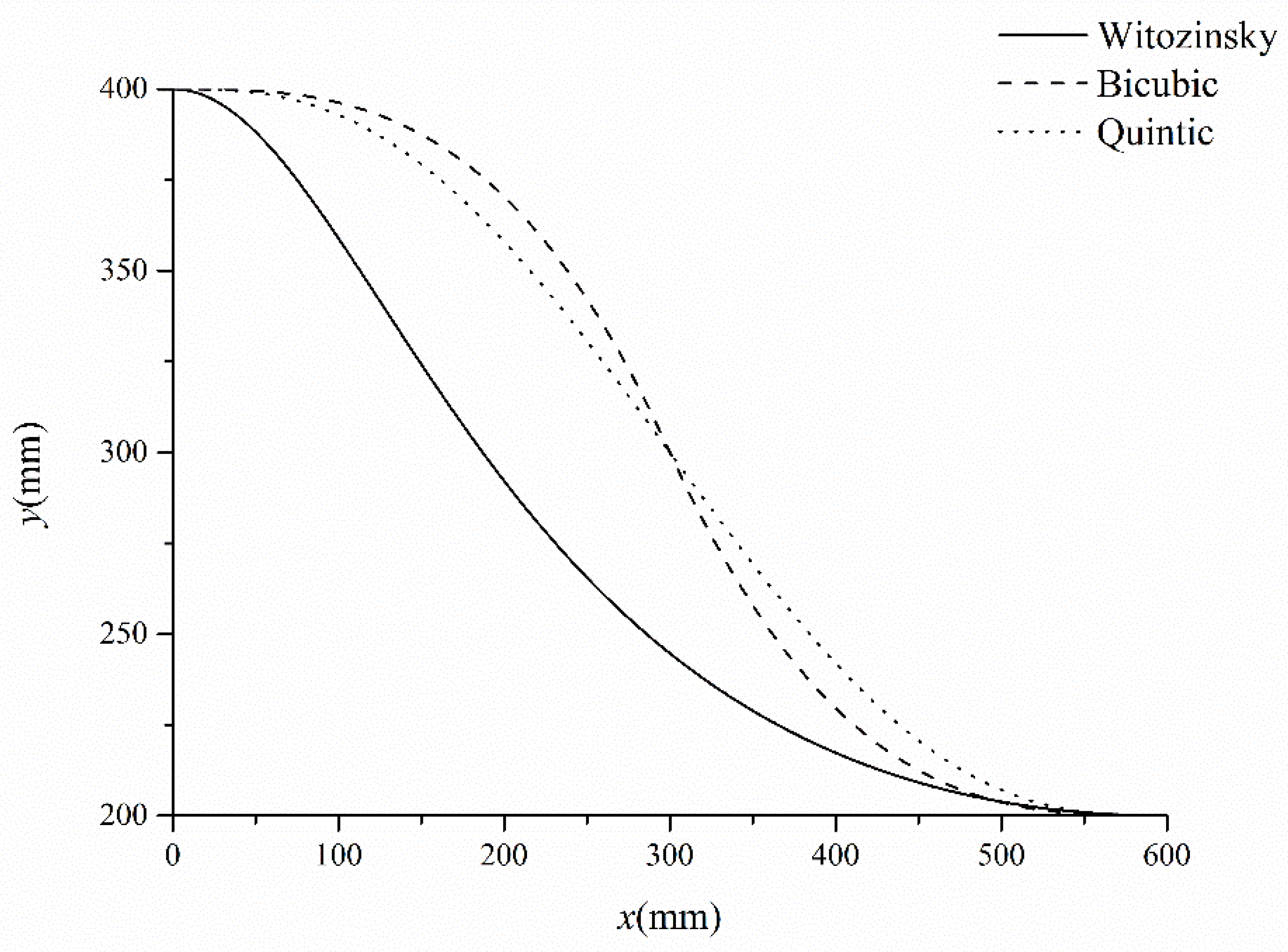
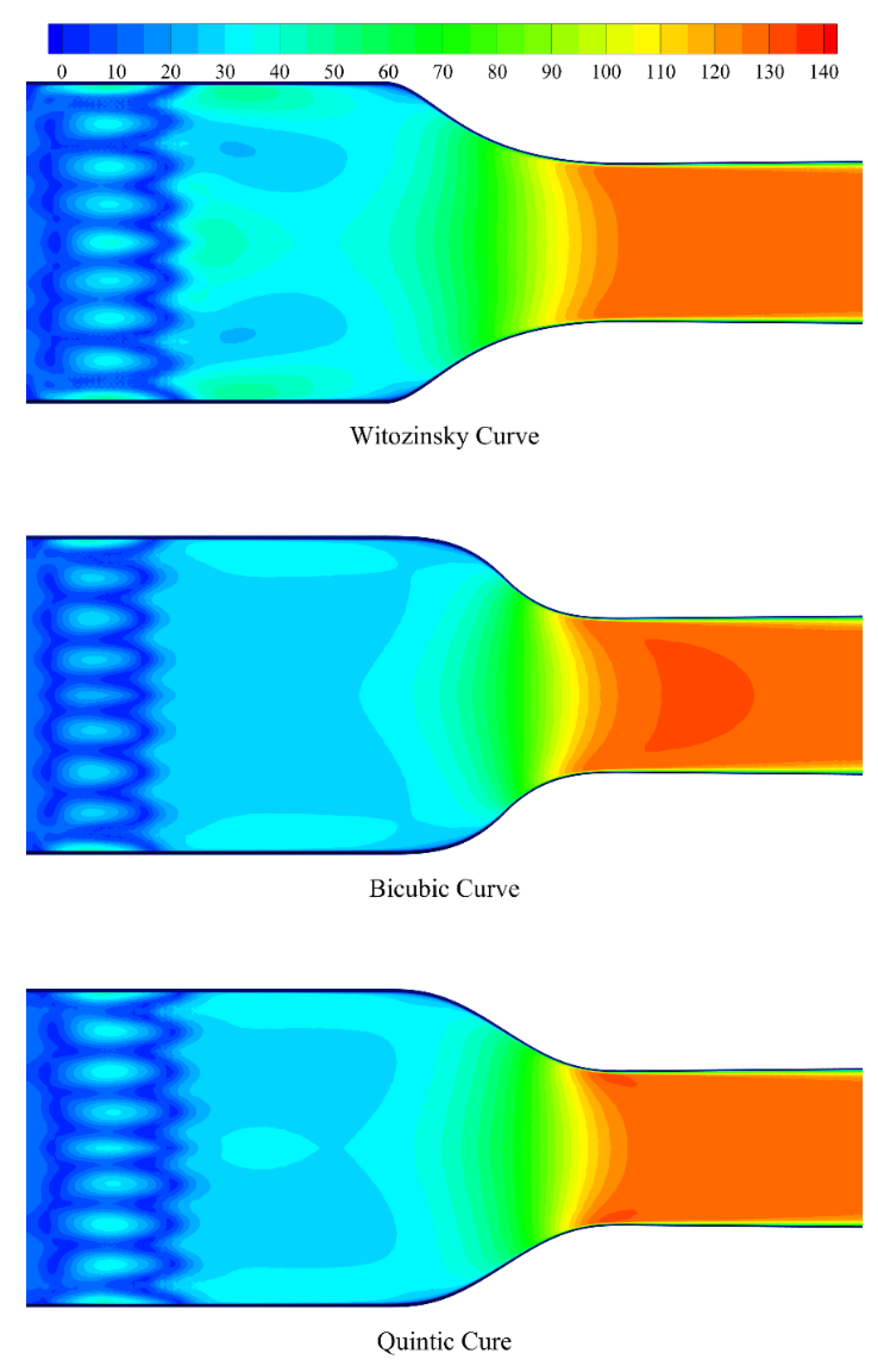
3.2. Contraction Curve
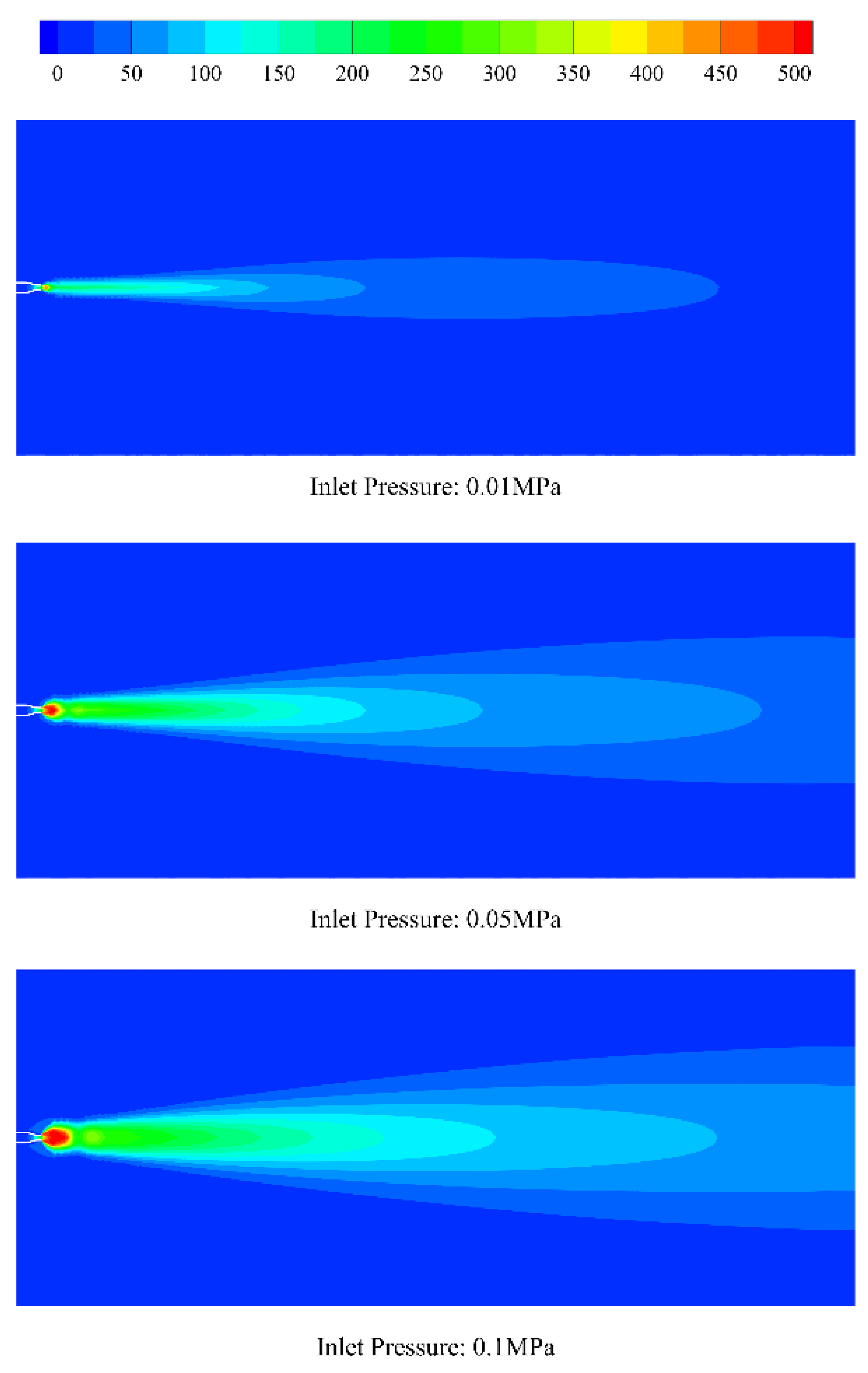
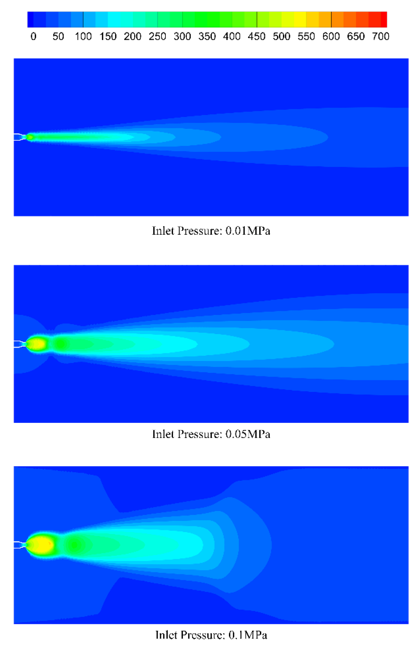
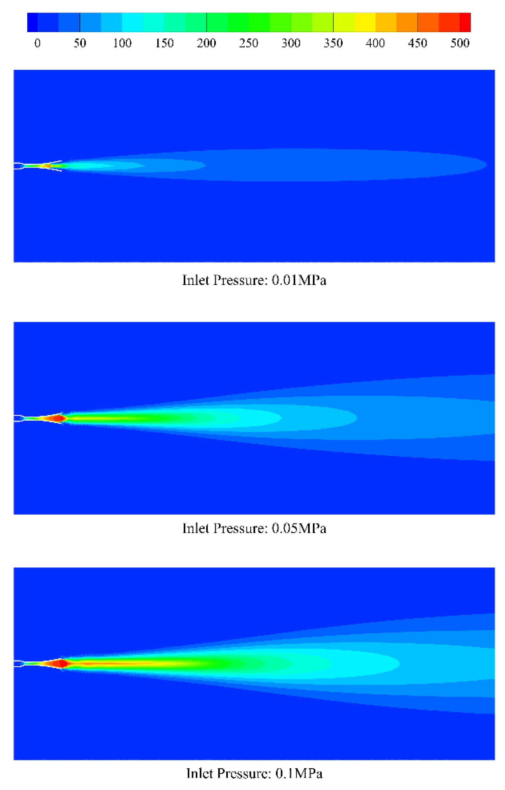
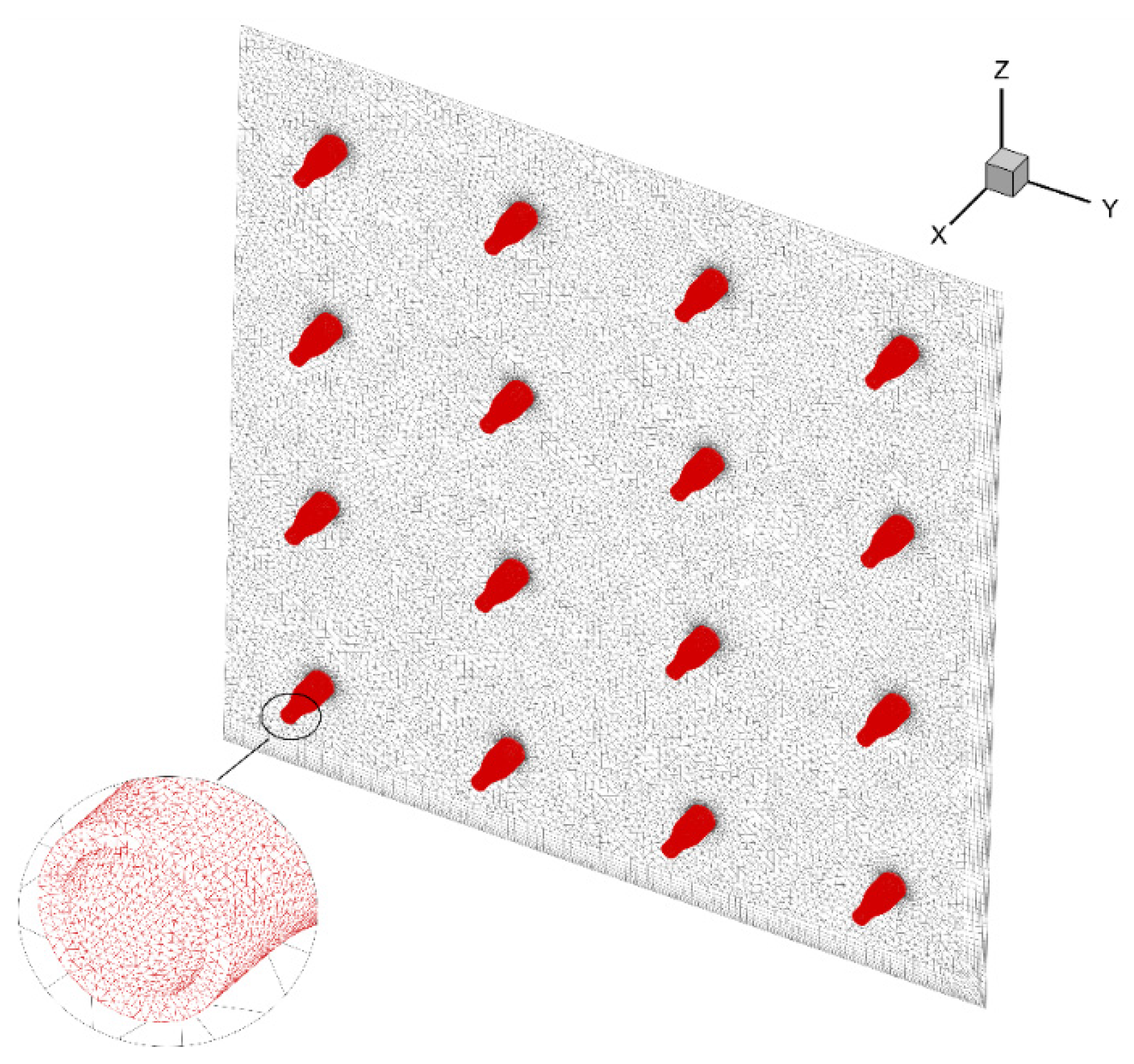
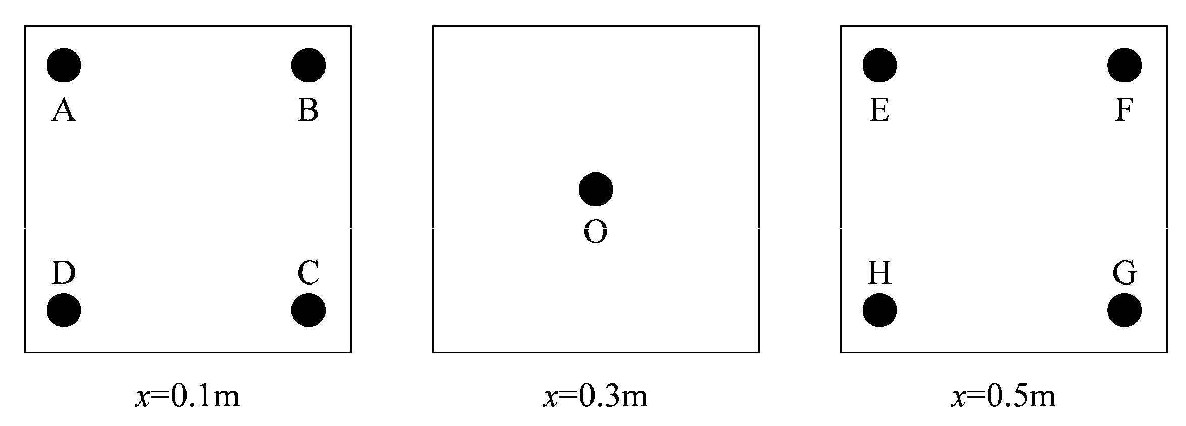
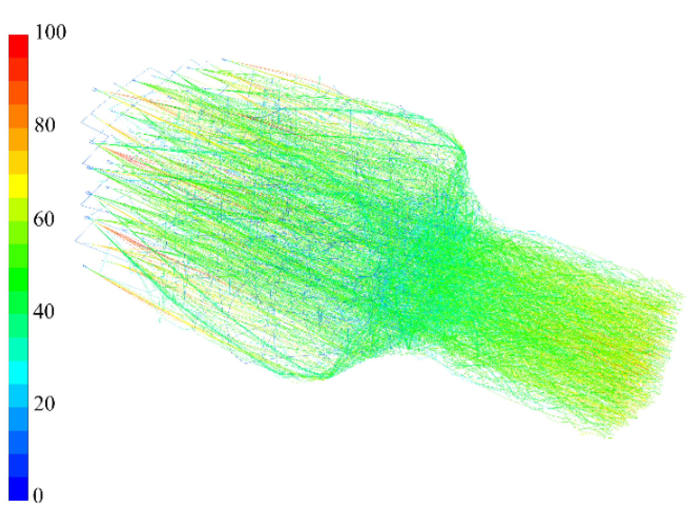
4. Two-Phase Flow Simulation
5. Conclusions
- ◆
- Optimizing the connection point of the bicubic curve to improve the flow field quality;
- ◆
- Designing experiments to validate the CFD simulation results;
- ◆
- Selecting other special particles to offset the influence of the earth’s gravity;
- ◆
- Designing the system control scheme.
Author Contributions
Funding
Data Availability Statement
Conflicts of Interest
References
- Rankin, A.; Maimone, M.; Biesiadecki, J.; Patel, N.; Levine, D.; Toupet, O. Driving curiosity: Mars rover mobility trends during the first seven years. In Proceedings of the 2020 IEEE Aerospace Conference, Big Sky, MT, USA, 7–14 March 2020; IEEE: Piscataway, NJ, USA, 2020. [Google Scholar] [CrossRef]
- Hoffman, T. InSight: Mission to mars. In Proceedings of the 2018 IEEE Aerospace Conference, Big Sky, MT, USA, 3–10 March 2018; IEEE: Piscataway, NJ, USA, 2018. [Google Scholar] [CrossRef]
- Witze, A. NASA’s Perseverance rover begins key search for life on Mars. Nature 2022, 606, 441–442. [Google Scholar] [CrossRef] [PubMed]
- Balaram, J.; Aung, M.; Golombek, M.P. The Ingenuity Helicopter on the Perseverance Rover. Space Sci. Rev. 2021, 217, 56. [Google Scholar] [CrossRef]
- Tian, H.; Zhang, T.; Jia, Y.; Peng, S.; Yan, C. Zhurong: Features and mission of China’s first Mars rover. Innovation 2021, 2, 100121. [Google Scholar] [CrossRef] [PubMed]
- Muirhead, B.K.; Nicholas, A.K.; Umland, J.; Sutherland, O.; Vijendran, S. Mars Sample Return Campaign Concept Status. Acta Astronaut. 2020, 176, 131–138. [Google Scholar] [CrossRef]
- Report of the 90-Day Study on Human Exploration of the Moon and Mars; NASA: Washington, DC, USA, 1989.
- Wang, X.; Wang, X. Research Progress and Preliminary Scheme of Space Transportation System for Human Mars Exploration. Aerosp. China 2021, 22, 3–14. [Google Scholar] [CrossRef]
- Imhof, B. [Interior] Configuration options, habitability and architectural aspects of the transfer habitat module (THM) and the surface habitat on Mars (SHM)/ESA’s AURORA human mission to Mars (HMM) study. Acta Astronaut. 2007, 60, 571–587. [Google Scholar] [CrossRef]
- Polsgrove, T.; Chapman, J.; Sutherlin, S.; Taylor, B.; Robertson, E.; Studak, B.; Vitalpur, S.; Fabisinski, L.; Lee, A.Y.; Collins, T.; et al. Human Mars lander design for NASA’s evolvable mars campaign. In Proceedings of the 2016 IEEE Aerospace Conference, Big Sky, MT, USA, 5–12 March 2016; pp. 1–15. [Google Scholar] [CrossRef]
- Barlow, N. Mars: An Introduction to Its Interior, Surface and Atmosphere, 1st ed.; Cambridge University Press: Cambridge, UK, 2008. [Google Scholar]
- Smith, P.H.; Bell, J.F.R.; Bridges, N.T.; Britt, D.T.; Gaddis, L.; Greeley, R.; Keller, H.U.; Herkenhoff, K.E.; Jaumann, R.; Johnson, J.R.; et al. Results from the Mars Pathfinder camera. Science 1997, 278, 1758–1765. [Google Scholar] [CrossRef]
- Kok, J.F.; Parteli, E.; Michaels, T.I.; Karam, D.B. The physics of wind-blown sand and dust. Rep. Prog. Phys. 2012, 75, 1–72. [Google Scholar] [CrossRef]
- Smith, M.D.; Pearl, J.C.; Conrath, B.J.; Christensen, P.R. Thermal Emission Spectrometer results: Mars atmospheric thermal structure and aerosol distribution. J. Geophys. Res.-Planets 2001, 106, 23929–23945. [Google Scholar] [CrossRef]
- Yan, Y.P.; Zou, M.; Yao, J.Y.; Yuan, B.F.; Lin, Y.C.; Jin, J.F. Endurance study of bionic wheels for Mars rovers. J. Terramechanics 2017, 74, 57–68. [Google Scholar] [CrossRef]
- Graser, E.; McGill, S.; Rankin, A.; Bielawiec, A. Rimmed Wheel Performance on the Mars Science Laboratory Scarecrow Rover. In Proceedings of the 2020 IEEE Aerospace Conference, Big Sky, MT, USA, 7–14 March 2020; pp. 1–12. [Google Scholar] [CrossRef]
- Landis, G.A. Dust obscuration of Mars solar arrays. Acta Astronaut. 1996, 38, 885–891. [Google Scholar] [CrossRef]
- Bridges, N.T.; Ayoub, F.; Avouac, J.P.; Leprince, S.; Lucas, A.; Mattson, S. Earth-like sand fluxes on Mars. Nature 2012, 485, 339–342. [Google Scholar] [CrossRef] [PubMed]
- Balme, M.; Greeley, R. Dust devils on Earth and Mars. Rev. Geophys. 2006, 44, 1–22. [Google Scholar] [CrossRef]
- Newman, C.E.; Hueso, R.; Lemmon, M.T.; Munguira, A.; Vicente-Retortillo, A.L.; Apestigue, V.I.C.; Mart, I.; Nez, G.A.N.M.; Toledo, D.; Sullivan, R.; et al. The dynamic atmospheric and aeolian environment of Jezero crater, Mars. Sci. Adv. 2022, 8, eabn3783. [Google Scholar] [CrossRef] [PubMed]
- Sullivan, R.; Arvidson, R.; Bell, J.F.; Gellert, R.; Golombek, M.; Greeley, R.; Herkenhoff, K.; Johnson, J.; Thompson, S.; Whelley, P.; et al. Wind-driven particle mobility on mars: Insights from Mars Exploration Rover observations at “El Dorado” and surroundings at Gusev Crater. J. Geophys. Res.-Planets 2008, 113. [Google Scholar] [CrossRef]
- Golombek, M.P.; Grant, J.A.; Crumpler, L.S.; Greeley, R.; Arvidson, R.E.; Bell, J.F.; Weitz, C.M.; Sullivan, R.; Christensen, P.R.; Soderblom, L.A.; et al. Erosion rates at the Mars Exploration Rover landing sites and long-term climate change on Mars. J. Geophys. Res.-Planets 2006, 111. [Google Scholar] [CrossRef]
- Calle, C.I.; Buhler, C.R.; Johansen, M.R.; Hogue, M.D.; Snyder, S.J. Active dust control and mitigation technology for lunar and Martian exploration. Acta Astronaut. 2011, 69, 1082–1088. [Google Scholar] [CrossRef]
- Trigwell, S.; Mazumder, M.K.; Biris, A.S.; Anderson, S.; Yurteri, C.U.; Mittal, K.L. Dust removal from solar panels and spacecraft on Mars. In Surface Contamination and Cleaning; CRC Press: Boca Raton, FL, USA, 2003; Volume 1, pp. 293–310. [Google Scholar]
- Kok, J.F.; Renno, N.O. Electrostatics in Wind-Blown Sand. Phys. Rev. Lett. 2008, 100, 014501. [Google Scholar] [CrossRef] [PubMed]
- Marshall, J.; Fenton, L.K.; Harlow, J. Limitations of applying grain weight similitude in aeolian studies with NASA Mars Wind Tunnel. Aeolian Res. 2021, 53, 100732. [Google Scholar] [CrossRef]
- Viúdez-Moreiras, D.; Gómez-Elvira, J.; Newman, C.E.; Navarro, S.; Marin, M.; Torres, J.; De La Torre-Juárez, M. Gale surface wind characterization based on the Mars Science Laboratory REMS dataset. Part II: Wind probability distributions. Icarus 2019, 319, 645–656. [Google Scholar] [CrossRef]
- Banfield, D.; Spiga, A.; Newman, C.; Forget, F.; Lemmon, M.; Lorenz, R.; Murdoch, N.; Viudez-Moreiras, D.; Pla-Garcia, J.; Garcia, R.F.; et al. The atmosphere of Mars as observed by InSight. Nat. Geosci. 2020, 13, 190–198. [Google Scholar] [CrossRef]
- Viúdez-Moreiras, D.; Newman, C.E.; Forget, F.; Lemmon, M.; Banfield, D.; Spiga, A.; Lepinette, A.; Rodriguez-Manfredi, J.A.; Gómez-Elvira, J.; Pla-García, J.; et al. Effects of a Large Dust Storm in the Near-Surface Atmosphere as Measured by InSight in Elysium Planitia, Mars. Comparison With Contemporaneous Measurements by Mars Science Laboratory. J. Geophys. Res. Planets 2020, 125, e2020JE006493. [Google Scholar] [CrossRef]
- J.P. Laboratory. Mars Dust Storms.; 1976. Available online: https://www.jpl.nasa.gov/news/mars-dust-storms (accessed on 3 October 2022).
- Papike, J.J. Planetary Materials; The Mineralogical Society of America: Chantilly, VA, USA, 1998. [Google Scholar]
- Kwiek, A. Conceptual design of an aircraft for Mars mission. Aircr. Eng. Aerosp. Technol. 2019, 91, 886–892. [Google Scholar] [CrossRef]
- Liu, T.; Oyama, A.; Fujii, K. Scaling Analysis of Propeller-Driven Aircraft for Mars Exploration. J. Aircr. 2013, 50, 1593–1604. [Google Scholar] [CrossRef]
- Greeley, R.; White, B.R.; Pollack, J.B.; Iverson, J.D.; Leach, R.N. Dust Storms on Mars: Considerations and Simulations; NASA: Washington, DC, USA, 1977.
- Dino, J. Mars Surface Wind Tunnel. 2008. Available online: https://www.nasa.gov/centers/ames/multimedia/images/2005/dust_devils.html (accessed on 30 August 2022).
- Gaier, J.R.; Perez-Davis, M.E.; Moinuddin, A.M. Effects of windblown dust on photovoltaic surface s on Mars. In Proceedings of the 26th Intersociety Energy Conversion Engineering Conference, Boston, MA, USA, 4–9 August 1991. [Google Scholar]
- Gaier, J.; De Leon, P.; Lee, P.; McCue, T.; Hodgson, E.; Thrasher, J. Preliminary testing of a pressurized space suit and candidate fabrics under simulated Mars dust storm and dust devil conditions. In Proceedings of the 40th International Conference on Environmental Systems, Barcelona, Spain, 11–15 July 2010. [Google Scholar]
- Merrison, J.P.; Gunnlaugsson, H.P.; Holstein-Rathlou, C.; Knak Jensen, S.; Mason, J.; Nørnberg, P.; Patel, M.; Portyankina, G.; Rasmussen, K.R. Latest results from the European mars simulation wind tunnel facility. In Proceedings of the EPSC-DPS Joint Meeting 2011, Nantes, France, 2–7 October 2011. [Google Scholar]
- Holstein-Rathlou, C.; Merrison, J.; Iversen, J.J.; Jakobsen, A.B.; Nicolajsen, R.; Nørnberg, P.; Rasmussen, K.; Merlone, A.; Lopardo, G.; Hudson, T.; et al. An environmental wind tunnel facility for testing meteorological sensor systems. J. Atmos. Ocean. Technol. 2014, 31, 447–457. [Google Scholar] [CrossRef]
- Merrison, J.P.; Bechtold, H.; Gunnlaugsson, H.; Jensen, A.; Kinch, K.; Nornberg, P.; Rasmussen, K. An environmental simulation wind tunnel for studying Aeolian transport on mars. Planet. Space Sci. 2008, 56, 426–437. [Google Scholar] [CrossRef]
- Greeley, R.; Leach, R.; White, B.; Iversen, J.; Pollack, J. Threshold windspeeds for sand on Mars—Wind tunnel simulations. Geophys. Res. Lett. 1980, 7, 121–124. [Google Scholar] [CrossRef]
- Franz, H.B.; Trainer, M.G.; Malespin, C.A.; Mahaffy, P.R.; Atreya, S.K.; Becker, R.H.; Benna, M.; Conrad, P.G.; Eigenbrode, J.L.; Freissinet, C.; et al. Initial SAM calibration gas experiments on Mars: Quadrupole mass spectrometer results and implications. Planet. Space Sci. 2017, 138, 44–54. [Google Scholar] [CrossRef]
- Wu, J.L.; Li, Z.H.; Peng, A.P.; Pi, X.C.; Li, Z.H. Numerical study on rarefied unsteady jet flow expanding into vacuum using the Gas-Kinetic Unified Algorithm. Comput. Fluids 2017, 155, 50–61. [Google Scholar] [CrossRef]
- Li, Y.H.; He, C.J.; Li, J.Q.; Miao, L.; Gao, R.Z.; Liang, J.M. Experimental investigation of flow separation in a planar convergent-divergent nozzle. In Proceedings of the 3rd International Conference on Fluid Mechanics and Industrial Applications (FMIA), Taiyun, China, 1 January 2019; Institute of Physics Publishing: Bristol, UK, 2019; p. 012088. [Google Scholar] [CrossRef]
- Wei, A.B.; Yu, L.Y.; Gao, R.; Zhang, W.; Zhang, X.B. Unsteady cloud cavitation mechanisms of liquid nitrogen in convergent-divergent nozzle. Phys. Fluids 2021, 33, 092116. [Google Scholar] [CrossRef]
- Cao, X.; Bian, J. Supersonic separation technology for natural gas processing: A review. Chem. Eng. Process.-Process Intensif. 2019, 136, 138–151. [Google Scholar] [CrossRef]
- Haider, A.; Levenspiel, O. Drag coefficient and terminal velocity of spherical and nonspherical particles. Powder Technol. 1989, 58, 63–70. [Google Scholar] [CrossRef]


| Items | Parameters |
|---|---|
| Gas medium | CO2 |
| Test section speed | 60~170 m/s |
| Static pressure | 600~1000 Pa |
| Test section temperature | 173~293 K |
| Particle diameter | 35~125 μm |
| Nozzle Type | Inlet Diameter | Outlet Diameter | Length | Throat Diameter | Convergent Angle | Divergent Angle | |
|---|---|---|---|---|---|---|---|
| 1# | Convergent nozzle | 10 mm | 4 mm | 30 mm | - | 11.8° | - |
| 2# | Convergent nozzle | 10 mm | 6 mm | 30 mm | - | 7.9° | - |
| 3# | Laval nozzle | 10 mm | 20 mm | 30 mm | 4 mm | 11.8° | 7.2° |
| Nozzle NO. | Inlet Pressure (MPa) | Nozzle Mass Flow Rate (kg/h) | Ejected Gas Flow Rate (kg/h) | Ejection Coefficient |
|---|---|---|---|---|
| 1# | 0.01 | 0.0004 | 0.0111 | 28.10 |
| 0.05 | 0.0020 | 0.0281 | 14.05 | |
| 0.10 | 0.0040 | 0.0418 | 10.45 | |
| 2# | 0.01 | 0.0016 | 0.0237 | 14.60 |
| 0.05 | 0.0082 | 0.0643 | 7.84 | |
| 0.10 | 0.0164 | 0.0802 | 4.89 | |
| 3# | 0.01 | 0.0004 | 0.0258 | 65.74 |
| 0.05 | 0.0020 | 0.0361 | 18.05 | |
| 0.10 | 0.0040 | 0.0395 | 9.875 |
| Witozinsky Curve | Bicubic Curve | Quintic Curve | |
|---|---|---|---|
| Max VI (%) | 1.43 | 1.16 | 1.14 |
| Max DPI (%) | 0.76 | 0.66 | 0.64 |
| Witozinsky Curve | Bicubic Curve | Quintic Curve | |
|---|---|---|---|
| ASPG (m−1) | 0.1376 | 0.1342 | 0.1845 |
| Inlet Pressure (MPa) | 0.01 | 0.05 | 0.1 |
|---|---|---|---|
| Average velocity (m/s) | 82.9 | 129.4 | 167.6 |
| Max VI | 0.40 | 0.66 | 1.06 |
| Max DPI (%) | 0.74 | 1.16 | 1.62 |
| ASPG (m−1) | 0.1293 | 0.1342 | 0.1347 |
Publisher’s Note: MDPI stays neutral with regard to jurisdictional claims in published maps and institutional affiliations. |
© 2022 by the authors. Licensee MDPI, Basel, Switzerland. This article is an open access article distributed under the terms and conditions of the Creative Commons Attribution (CC BY) license (https://creativecommons.org/licenses/by/4.0/).
Share and Cite
Wu, H.; Liu, M.; Mi, Y.; Wang, J.; Guo, M. Key Parameters of a Design for a Novel Reflux Subsonic Low-Density Dust Wind Tunnel. Aerospace 2022, 9, 662. https://doi.org/10.3390/aerospace9110662
Wu H, Liu M, Mi Y, Wang J, Guo M. Key Parameters of a Design for a Novel Reflux Subsonic Low-Density Dust Wind Tunnel. Aerospace. 2022; 9(11):662. https://doi.org/10.3390/aerospace9110662
Chicago/Turabian StyleWu, Hao, Meng Liu, Youzhi Mi, Jun Wang, and Menglei Guo. 2022. "Key Parameters of a Design for a Novel Reflux Subsonic Low-Density Dust Wind Tunnel" Aerospace 9, no. 11: 662. https://doi.org/10.3390/aerospace9110662
APA StyleWu, H., Liu, M., Mi, Y., Wang, J., & Guo, M. (2022). Key Parameters of a Design for a Novel Reflux Subsonic Low-Density Dust Wind Tunnel. Aerospace, 9(11), 662. https://doi.org/10.3390/aerospace9110662