
Aerodynamic Characteristics of a Ducted Fan Hovering and Transition in Ground Effect

School of Aeronautic Science and Engineering, Beihang University, Beijing 100191, China
*
Author to whom correspondence should be addressed.
Aerospace 2022, 9(10), 572; https://doi.org/10.3390/aerospace9100572
Submission received: 15 September 2022
/
Revised: 28 September 2022
/
Accepted: 28 September 2022
/
Published: 30 September 2022
Abstract
:Ducted fans installed on vertical takeoff and landing vehicles experience significant ground effect during takeoff and landing. The aerodynamic characteristics of a ducted fan hovering and transitioning in the ground effect are studied using numerical simulations in this paper. The flowfields are obtained by solving Reynolds Averaged Navier–Stokes equations with the Multiple Reference Frame approach. When a ducted fan hovers in the ground effect, the blade thrust increases due to the combined effect of the increase in the effective angle of attack of the blade and the increase in ambient pressure; the duct thrust decreases due to the combined effect of the decrease in the effective angle of attack of the duct and the increase in ambient pressure. Stall occurs at a certain advance ratio and angle of attack when transitioning in the ground effect. The ground effect delays the occurrence of stall at some advance ratios. The ground effect is hardly detectable at angles of attack less than 30° even if the height drops to 0.5 times the duct exit diameter. At this height and high angles of attack, the different positions and influence regions of the ground vortex at different advance ratios contribute to the different variation trends in the ducted fan performance.
1. Introduction
Ducted fans can generate more static thrust when compared to open propellers of the same diameter and power loading [1]. In addition, the duct serves as a safety feature, protecting both the rotating blades from damage by other objects as well as personnel from injury by the blades. Moreover, ducted fans have advantages in noise suppression and thrust vectoring. These characteristics make the ducted fan an appropriate propulsion system for vertical/short takeoff and landing (V/STOL) aircraft. In the 1960s, research institutions such as National Aeronautics and Space Administration (NASA) carried out systematic studies on ducted-fan-propelled V/STOL aircraft. Some research aircraft developed during this period, for example, the Doak VZ-4 [2] and the Bell X-22A [3], even completed successful flight tests. Nowadays, within the aviation industry there is a strong and growing interest in the development of electric vertical takeoff and landing (eVTOL) aircraft for various potential applications, especially for Urban Air Mobility (UAM) missions. Many eVTOL aircraft, such as the Bell Nexus [4], Lilium Jet [5], and NASA UAM reference tilt duct vehicle [6], use ducted fans as propulsion systems due to their above-mentioned advantages. According to previous studies, most of the V/STOL aircraft suffer from some degree of an adverse ground effect during takeoff and landing [2]. Therefore, it is necessary to study the aerodynamic characteristics of ducted fans in the ground effect, which can provide support for improving the performance of ducted-fan-propelled V/STOL aircraft in the ground effect.
Ducted fans were first studied in the 1930s [7]. Sacks and Burnell [7] compiled an exhaustive survey of the theoretical and experimental research up to 1962. Mort and Yaggy [8] studied the aerodynamic characteristics of a wingtip-mounted ducted fan. Large nose-up pitching moments and duct stall were observed when the ducted fan operated at nonzero angles of attack. Grunwald and Goodson [9] investigated the division of loads between the fan and the duct of an isolated ducted fan. They verified that the duct could provide more than half of the thrust in hover and could carry even more of the load in forward flight at a certain angle of attack. Mort and Gamse [10] measured the forces, pressure, power, figure of merit, propulsive efficiency, and stall limits of a 7-foot-diameter ducted fan under various conditions, intending to evaluate the quality of the ducted fan design. Abrego and Bulaga [11] completed an experimental investigation to determine the performance of a ducted fan model with different duct geometries. Model variations included the duct’s angle of attack, the exit vane flap length, the flap deflection angle, and the duct’s chord length. Martin and Tung [12] measured the performance and flowfield of a ducted fan, with emphasis on the tip gap and duct lip shape effects. The experimental results were later compared to panel method calculations by Lind et al. [13]. Good correlations within the attached flow region were achieved. Graf et al. [14] studied the effect of duct lip shape on ducted fan performances. They found that flow separation characteristics on the inside of the duct lip caused the performance difference between the duct geometries. Pereira [15] experimentally studied the effects of duct profile shapes on the performance of small-scale ducted fans. Tests performed for a specific ducted fan model at angles of attack from 0° to 90° and various advance ratios were also reported. Colman et al. [16] provided the force and moment data of an axial asymmetric ducted fan with cyclic pitch actuation. The duct with circumferentially varying airfoil sections was used to improve the cruise efficiency. Hrishikeshavan and Chopra [17] studied the response of a ducted fan to edgewise gusts by means of experiments and flight tests. Ohanian et al. [18] modeled the aerodynamic terms of an axisymmetric ducted fan configuration with twelve nondimensional coefficients. This modeling technique attains very high correlation for typical ducted fan flight conditions. Cai et al. [19] evaluated the unsteady aerodynamics of a sinusoidal pitching ducted fan UAV using an unstructured overset grid technique and momentum source method. Ryu et al. [20] analyzed the aerodynamic performance of a ducted fan in crosswinds, covering an angle of attack ranging from −30° to 120°. No lip separation was observed in Ryu’s study due to the relatively large duct lip radius and the small advance ratios. Raeisi and Alighanbari [21,22] carried out experiments and CFD simulations to investigate the advantages of using an asymmetrical tilting ducted fan instead of a symmetrical one. They found that the asymmetrical duct can provide more lift and smaller force fluctuations during the transition from hovering to cruise. Misiorowski et al. [23] analyzed the forces, moments, and their decomposition on a ducted fan in edgewise flight along with a detailed analysis of the flow physics. Deng et al. [24] conducted experiments on a coaxial ducted fan UAV under forward flight conditions and successfully defined an initial operation region of the UAV. Akturk and Camci [25] identified the aerodynamic modifications due to fan inlet flow distortion in edgewise flight and then proposed a method using a secondary duct to control the inlet lip separation during edgewise flight.
Recently, Zhang and Barakos [26] provided another survey of published works on ducted fans since the 1960s. Experiments, theoretical studies, low-order methods and high-fidelity CFD simulations were reviewed. Studies related to ducted fans in the ground effect are not included in Zhang’s paper. There are relatively few studies on the aerodynamics of ducted fans in the ground effect in the literature. Giulianetti et al. [27] measured the performance parameters in the ground effect of a large-scale model of a V/STOL aircraft having four tilting ducted fans arranged in tandem pairs, but the parameters of the ducted fans were not measured separately. Divitiis [28], Hosseini et al. [29], and Ai et al. [30] developed different lower-order aerodynamic models of ducted fans considering the ground effect for online flight control. Gourdain et al. [31] investigated the influence of a duct on the rotor/ground interaction. The main objective of Gourdain’s study was to validate the capability of a lattice-Boltzmann-based large eddy simulation to reproduce the flow generated by the rotor/ground interaction. Deng et al. [26,32] measured and analyzed the aerodynamic performances of coaxial ducted fans hovering in the ground effect. Deng [33] measured the thrust and power of a ducted fan with different pitch angles at different heights in the ground effect. Han et al. [34] conducted experimental measurements and CFD simulations to study the aerodynamic performance of a micro-scale ducted fan hovering in a confined environment, including the ground, ceilings, and walls. Jin et al. [35] estimated the aerodynamic stability of a ducted fan in the ground effect with a modified Moore–Greitzer model. Han et al. [36] compared the performance and flowfield characteristics of a ducted fan and an open propeller hovering in the ground effect by means of experiments and CFD simulations. They found that the aerodynamic performance of the ducted fan was more sensitive to the ground effect than that of the open propeller. Mi [37] numerically investigated the effects of the ground, static water, and dynamic waves on the aerodynamic performance of a ducted fan. The results show that the water effect is weaker than the ground effect, and the dynamic waves have the most complicated effect on the ducted fan.
From the above review, it can be seen that previous studies mainly focus on the impact of geometric parameters and freestream conditions on the aerodynamic performance of ducted fans. Studies related to the ground effect mainly focus on the variation law of aerodynamic performance with height when a ducted fan hovers in the ground effect, but the mechanism of the ground effect lacks in-depth research. In addition, studies on the aerodynamic characteristics of ducted fans transitioning in the ground effect have been very limited. When ducted-fan-propelled V/STOL aircraft take off and land vertically or run on the ground in STOL mode, the ducted fans will experience significant influences of the ground effect. In view of the above-mentioned considerations, the aerodynamic characteristics of a ducted fan hovering and transitioning in the ground effect are studied using numerical simulations in this paper. The variation trends in the aerodynamic performance of the ducted fan are analyzed, and the flow physics leading to these trends are revealed.
2. Numerical Method and Validation
2.1. Ducted Fan Model
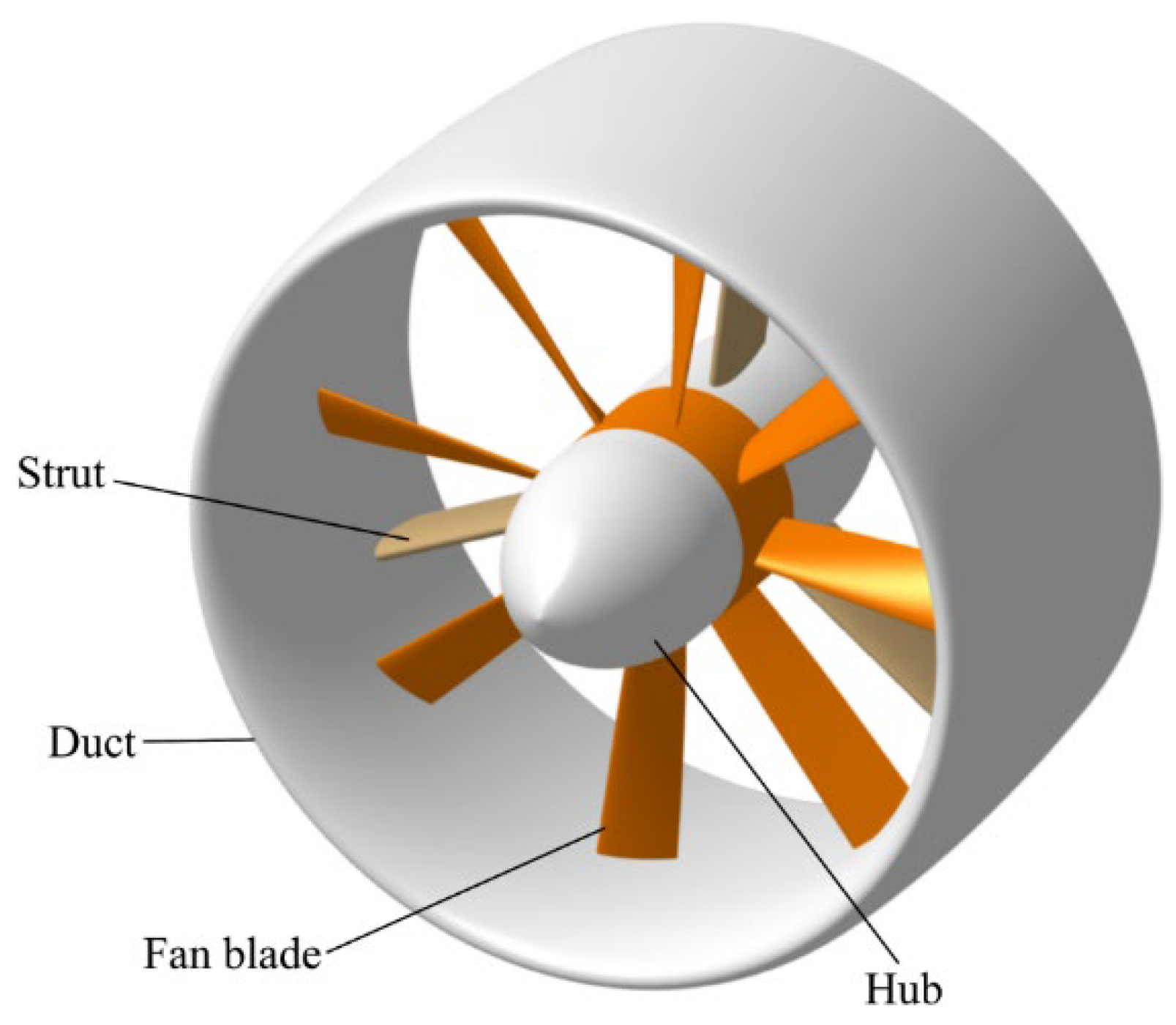
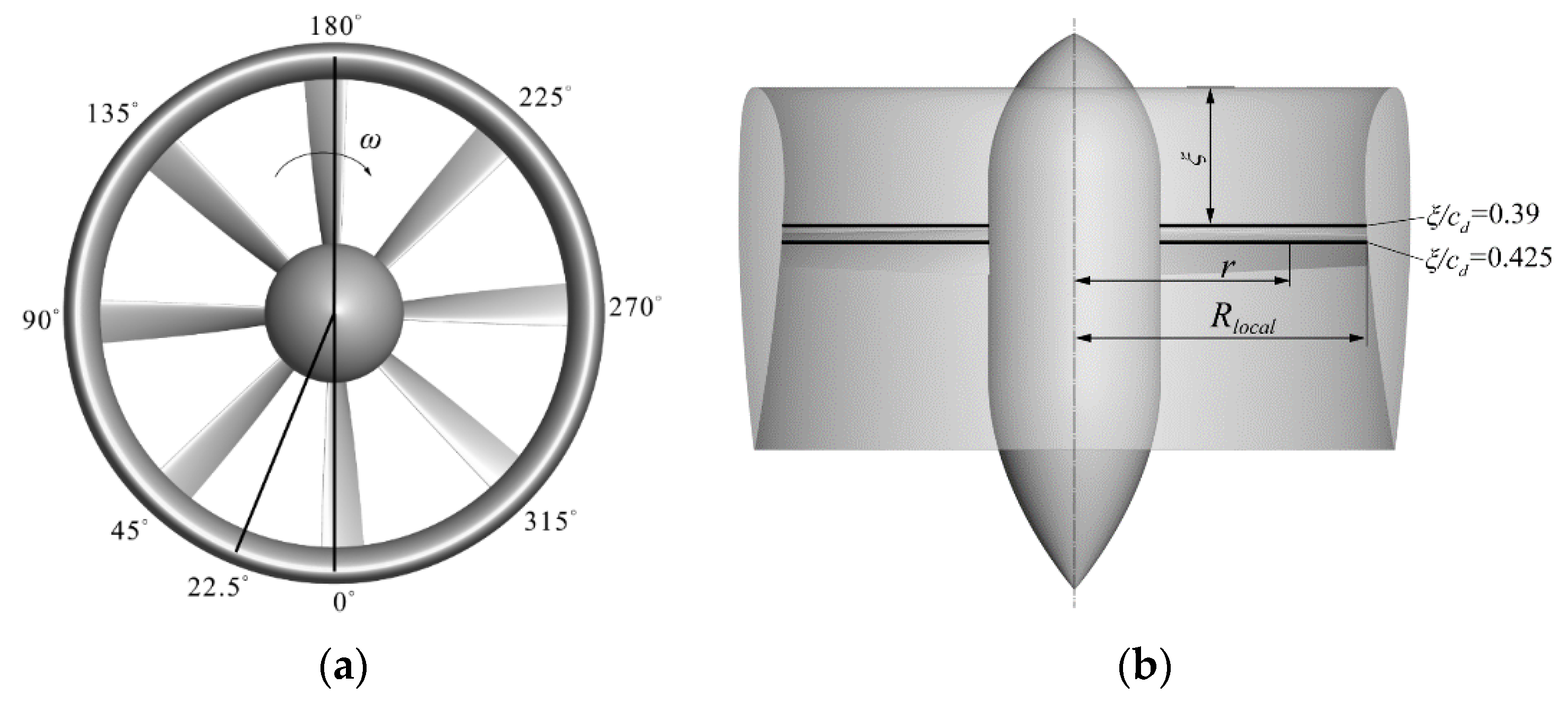
The ducted fan used in this study is shown in Figure 1. It is composed of a duct, fan blades, a hub, and struts. It should be noted that the struts are ignored in the numerical models. Details of the ducted fan are summarized in Table 1. The chord and twist distributions of the blade are plotted in Figure 2. The quarter-chord line of the blade is perpendicular to its rotation axis. When the blade is installed on the hub, its quarter-chord line is located at 42.5% of the duct chord. The ducted fan can generate 84 kgf static thrust with a fan rotational speed of 3500 revolutions per minute (rpm), and it is a 5/8 scale model of a ducted fan used for an eVTOL aircraft with a maximum takeoff weight of 3000 kg.
2.2. Validation of Numerical Method
The coordinate system used in this study has its origin at the intersection of the fan rotation axis with the blade quarter-chord line. All moments were referenced to this origin. The coordinate system followed the right-hand rule. Figure 3 illustrates the coordinate axes and the positive directions of the velocity, angle of attack, forces, and moments.
The nondimensional coefficients defined by Equations (1)–(8) were used in the subsequent analysis:
The Multiple Reference Frame (MRF) method was used to simulate the fan rotation in this study. The MRF method required two separate zones connected by frame interfaces inside the computational domain: the rotating zone containing the block near blades and the stationary zone containing the rest block, as shown in Figure 4. The computational domain was a cuboid with lengths of 100D, 50D, and 100D in the flow, normal, and span directions, respectively. Out of the ground effect simulations, the most downstream farfield boundary was set as the pressure outlet, with a gauge pressure of 0 Pa relative to the reference pressure p∞; the other boundaries were set as velocity inlets, which were specified to have the same velocity as the freestream. All surfaces of the ducted fan were set as no-slip walls. Trial simulations showed that if the pressure inlet was replaced by a velocity inlet of 0.5 m/s at the corresponding farfield boundaries, the discrepancies between the calculated thrust and torque were within 1%, but the order of magnitude of the maximum residual reduced from 10−3 to 10−5, as shown in Figure 5. Thus, a velocity of 0.5 m/s was specified on the velocity inlet boundaries when simulating the ducted fan hovering in still air. The air was assumed to be ideal gas with a constant dynamic viscosity μ = 1.7894 × 10⁻⁵. The CFD software STAR CCM+ was adopted to perform the numerical simulations. The Realizable k-ε turbulence model with two-layer all y+ wall treatment was used in all simulations. The other options remained the default settings of the software [38].
The experiment conducted by Grunwald [9] was chosen for CFD validation, because the ducted fan studied in this paper has no experimental data yet. The ducted fan used in Grunwald’s experiment, hereafter labeled as Grunwald’s model, consists of a three-blade fan with a diameter of 0.381 m, a hub with a diameter of 0.109 m, and a duct with a chord length of 0.261 m. The tip clearance is 0.53%Rb. Since the tip clearance is very small, to resolve it, the number of meshes as well as the difficulty of mesh generation is increased. According to the method proposed by Bunker [39], ignoring the tip clearance will overestimate the ducted fan performance, in terms of propulsion efficiency, by about 0.9%. This discrepancy is acceptable for the present study. Therefore, the tip clearance is ignored in the subsequent simulations. To perform the grid independence study, three sets of polyhedral meshes were generated: the coarse, medium, and fine mesh with 4.44 million, 8.86 million, and 16.6 million cells, respectively. The grid refinement was mainly performed on the ducted fan surfaces and the spherical region with a diameter of 5D surrounding the ducted fan. The flowfield near walls was calculated by a wall function, and thus the first layer height of the grid was taken to make the y+ value between 30 and 200 [38]. The fan rotational speed was set to ω = 8000 rpm in simulations of Grunwald’s model. Firstly, the case of hovering was simulated. The thrust and torque coefficients calculated with different grid densities are plotted in Figure 6. The discrepancy between the torque coefficient calculated by the coarse mesh and that calculated by the medium mesh is 7.1%. However, the discrepancies between the coefficients calculated by the medium mesh and those calculated by the fine mesh are all within 1%. The comparison between the CFD results of the medium mesh and the experimental values is shown in Table 2. It can be seen that all discrepancies are within 8%, indicating that the CFD results agree well with the experimental values. The calculation accuracy in this study is comparable to that of Qing et al. [40]. In the results of Qing, the discrepancy of CT, total is 7.06%, and the discrepancy of CQ is −3.05%.
Then, the case of J = 0.595, α = 30° was simulated with the medium mesh, and the results are shown in Table 3. It should be noted that the coefficients in Table 3 were calculated by the method defined in Grunwald’s report [9], which means that CL, CX, and CM were nondimensionalized based on the dynamic pressure of the freestream. The discrepancies between the calculated and experimental values of all coefficients are within 10%, and this means that the medium mesh can achieve acceptable accuracy. The results of these two cases also show that the numerical model established in this paper can be used to analyze the aerodynamic performance of ducted fans under different freestream conditions.
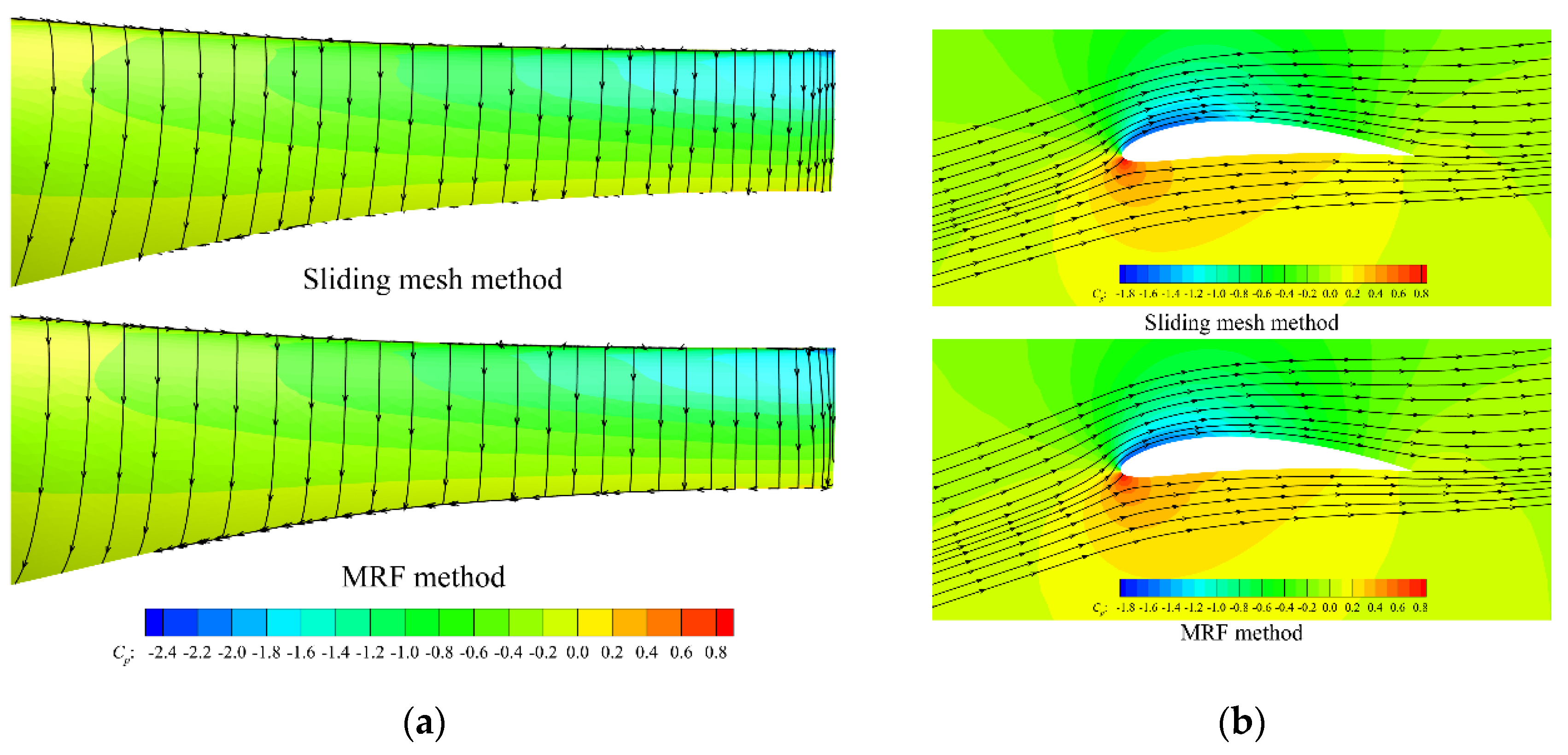
To further verify the appropriateness of the MRF method, the results of hovering out of the ground effect were compared with those obtained via the sliding mesh method (SMM). While performing the sliding mesh simulation, the implicit unsteady solver was selected; the temporal discretization was set to second order; the time step was set to Δt = 2.083 × 10⁻⁵ s, corresponding to a rotation of 1° per time step; and the maximum inner iterations within a time step was set to 20. The comparison between the aerodynamic coefficients obtained via the MRF method, the sliding mesh method, and the experiment is shown in Table 4. As can be seen, the results of the sliding mesh method are closer to the experimental values. However, the sliding mesh method took about 10 times more CPU time than the MRF method in this case. Figure 7 shows the limiting streamlines on the suction side of the blade and streamlines on the cross section very close to the blade tip. As can be seen in Figure 7a, the streamline patterns obtained by these two methods are only slightly different in the area immediately adjacent to the blade tip. This indicates that, for the current simulation, the flow field obtained via the MRF method is similar to that obtained via the sliding mesh method. In general, the accuracy of the MRF method is sufficient to support the flow field analysis in this study.
To the best of our knowledge, there are currently no experiments on the ground effect of ducted fans available for numerical method validation in the public literature, because it is difficult to accurately recreate the geometric models used in the experiments. The MRF-based RANS solver was used to calculate the aerodynamic performances of ducted fans in the ground effect in Han’s study [36]. In Han’s study, the discrepancies between the calculated coefficients and the experimental values are less than 10%, considering the 5% uncertainties in the measurements. This indicates that the MRF-based RANS solver can achieve acceptable accuracy when calculating the aerodynamic performance of ducted fans in the ground effect.
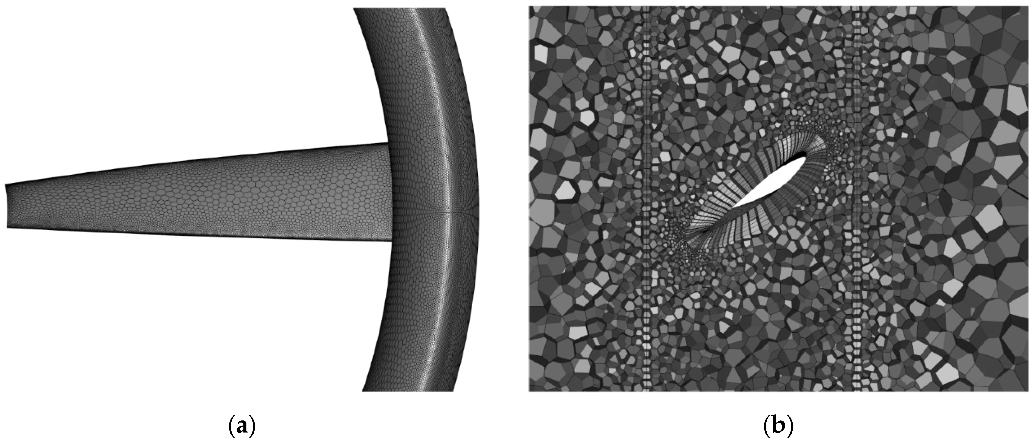
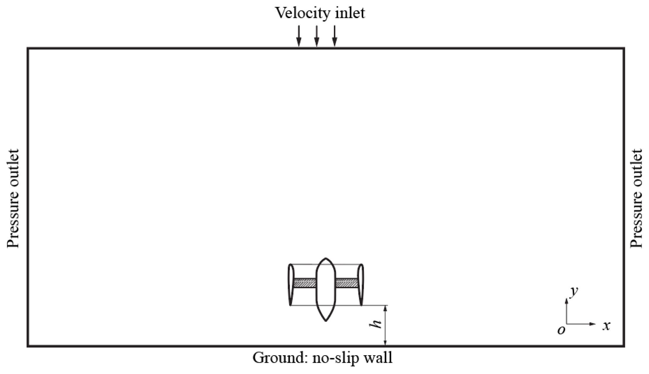
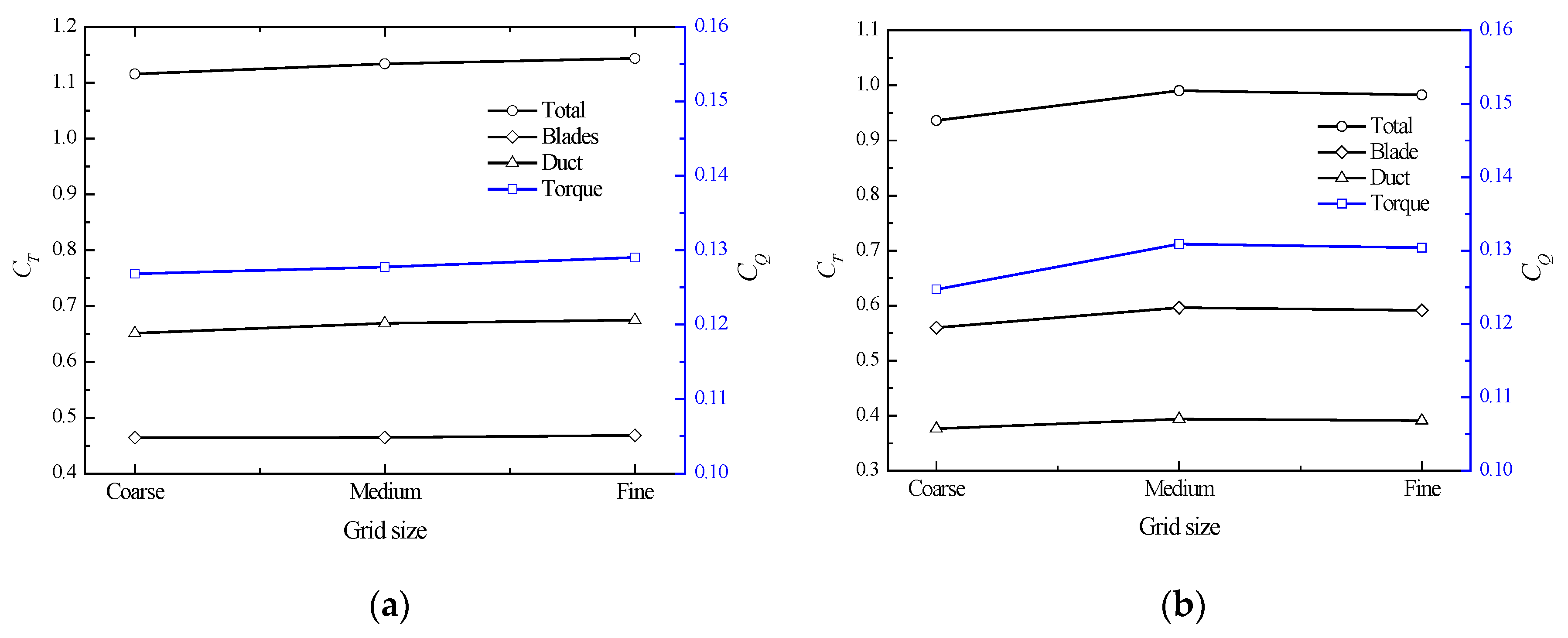
To perform a grid independence study for the ducted fan studied in this paper, three sets of meshes for simulations out of the ground effect were generated using control parameters similar to those used in the meshing of Grunwald’s model. The cell numbers were 4.71 million, 8.79 million, and 16.8 million and were labeled as coarse, medium, and fine mesh, respectively. Figure 8 shows some surface and cross section meshes of the medium mesh. The same surface meshes of the ducted fan were used to generate the volume meshes for the ground effect simulations. Another three sets of meshes with the number of 3.74 million, 6.25 million, and 14.9 million were obtained. The first-layer height of the grid was taken to make the y+ value at the three-quarter radius of the blade the same as that of Grunwald’s model. The fan rotational speed was set to ω = 3500 rpm. At this rotational speed, the blade tip Mach number was 0.35 and the Reynolds number based on the chord length at the three-quarter radius and tip speed was Re = 5.2 × 10⁵. The two cases of hovering in and out of the ground effect were simulated. The boundary conditions used while performing simulations of the ducted fan hovering in the ground effect are shown in Figure 9: the bottom surface was set as the non-slip wall; the four side surfaces were set as pressure outlets with a gauge pressure of 0 Pa relative to the reference pressure p∞; the top surface was set as the velocity inlet, and a velocity of 0.5 m/s was imposed on it to reduce the order of magnitude of the residuals, as mentioned above. The results are shown in Figure 10. The maximum discrepancy between the coefficients calculated using the coarse mesh and those calculated using the fine mesh was 5.3%, while the discrepancies between coefficients calculated using the medium mesh and those calculated using the fine mesh were all within 1%. Therefore, the medium mesh was used for subsequent simulations, and the other meshes used in this study were generated according to the medium one.
3. Hovering in Ground Effect
In this section, the aerodynamic characteristics of the ducted fan hovering in the ground effect are studied, which may happen when a ducted fan UAV hovers near the ground or when a ducted-fan-propelled V/STOL aircraft takes off and lands vertically. The numerical method established in Section 2.2 was used to perform simulations of the ducted fan hovering in the ground effect. According to Han’s [36] study, the aerodynamic coefficients almost keep constant at a given height in a large rotational speed range when a ducted fan hovers near the ground. Therefore, the following simulations were all performed at a constant rotational speed of 3500 rpm.
3.1. Variation in Ducted Fan Performance with Height
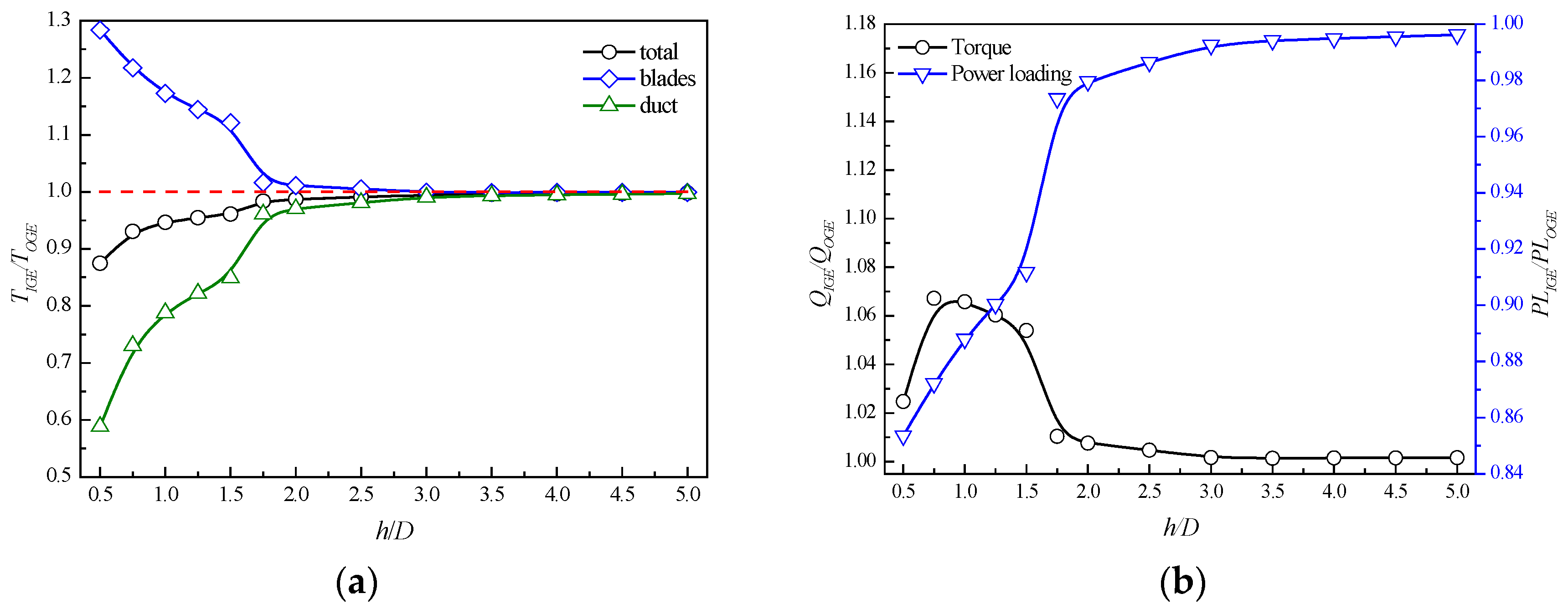
The aerodynamic performance of the ducted fan in the height range of 0.5D−5D was calculated. The calculation interval was 0.25D in the height range of 0.5D−2D and 0.5D in the height range of 2D−5D. All forces and moments converged to constant values after sufficient iterations. The results are plotted in Figure 11. The values of the thrust, torque, and power loading in the ground effect were normalized by the corresponding values out of the ground effect, which are presented in Table 5. It can be seen that the ground effect is negligible when the height off the ground is greater than 3D. The ground effect becomes significant when the height is less than 1.5D, within which the thrust changes in the duct and the blades are both above 10%. As the height decreases, the thrust of the blade increases, while the thrust of the duct decreases. Compared with the values out of the ground effect, at the height of 0.5D, the thrust of the blades increases by 28.4%, and the thrust of the duct decreases by 41.1%, resulting in a total thrust decrease by 12.5%. The conclusion that ground effect increases blade thrust but decreases duct thrust has been unanimously recognized in the literature. However, some studies [29,30,32,34,36] found an increase in total thrust, while other studies [33,37] found a decrease in total thrust. The key is whether the increment in the blade thrust can compensate for the loss of the duct thrust. In the study of Mi [37] and this paper, the ratio of the duct thrust to the total thrust is greater than 50% when the ducted fan hovers out of the ground effect, while this ratio is less than 50% in Han’s studies [34,36]. It is reasonable to infer that whether the total thrust of a ducted fan increases or decreases is related to the proportion of thrust generated by the duct and the blades when out of the ground effect. As shown in Figure 11b, the blade torque increases slightly in the ground effect, with a maximum increase of 7% at the height of 0.75D. The power loading decreases due to the increase in the shaft power and the decrease in the total thrust, and it decreases by 14.6% at the height of 0.5D. This means that the efficiency of the ducted fan will decrease in the ground effect.
3.2. Flow Physics Leading to Increase in Blade Thrust
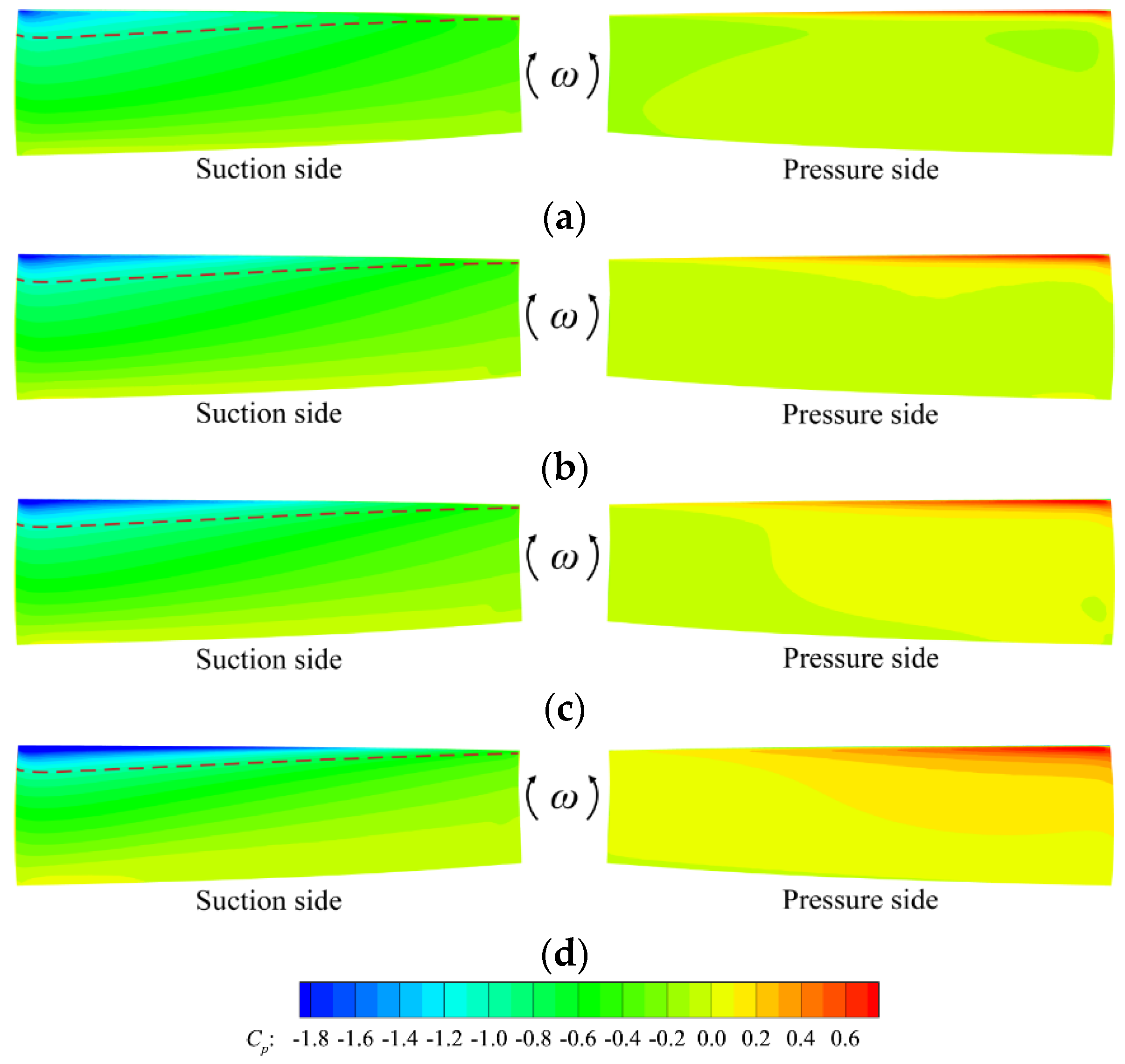
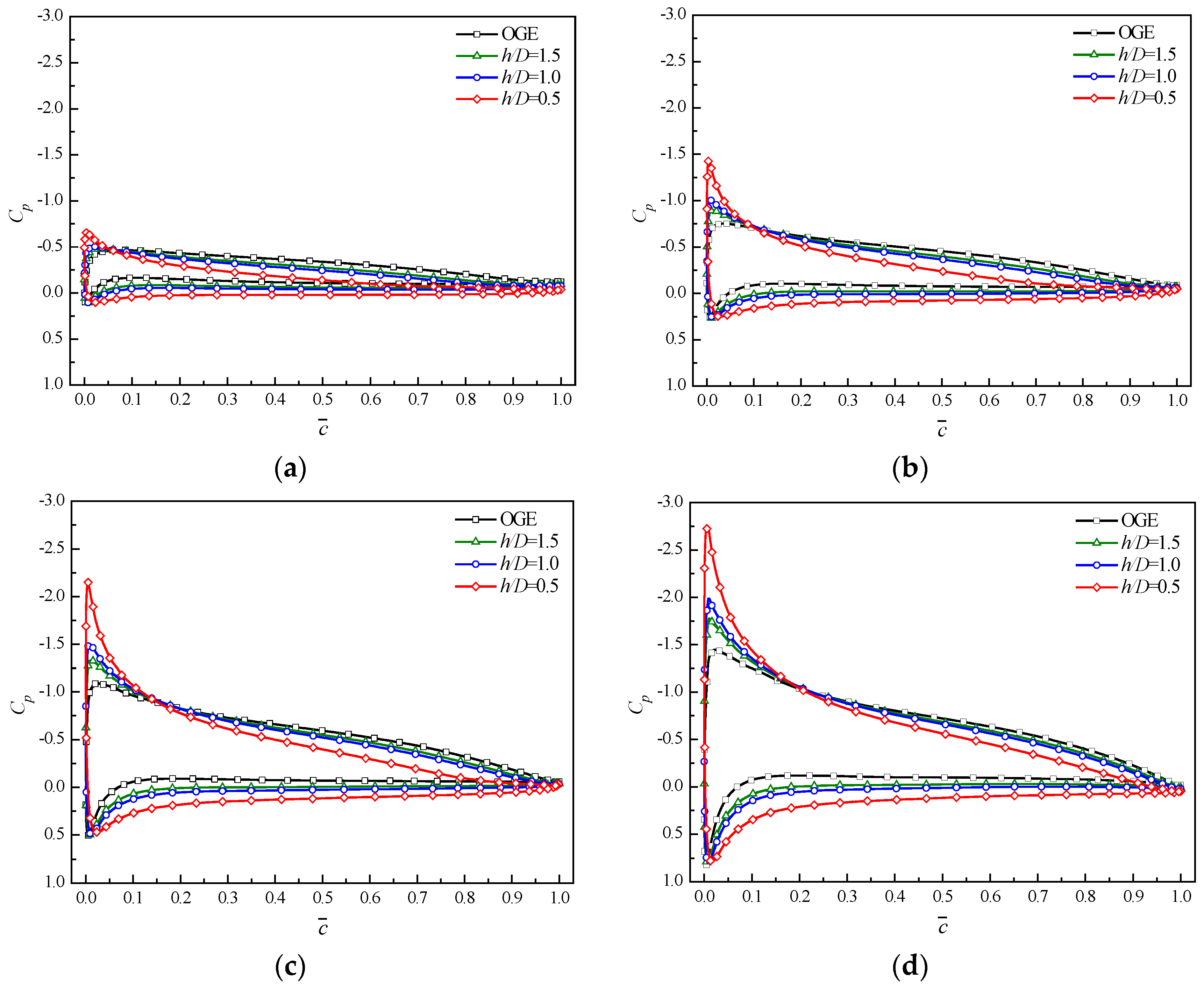
Figure 12 shows the pressure coefficient contours on blade surfaces at different heights, and Figure 13 shows the chordwise pressure coefficient distributions at different radial locations. When the ducted fan approaches the ground, the pressure on the pressure side of the blade increases, while the pressure on the suction side of the blade decreases in the area before the red dotted line and increases in the other area, as shown in Figure 12. This is also reflected in Figure 13. Taking Figure 13b as an example, at r/Rb = 0.55, the pressure on the suction side decreases as the height decreases before , and then, the pressure increases as the height decreases after .
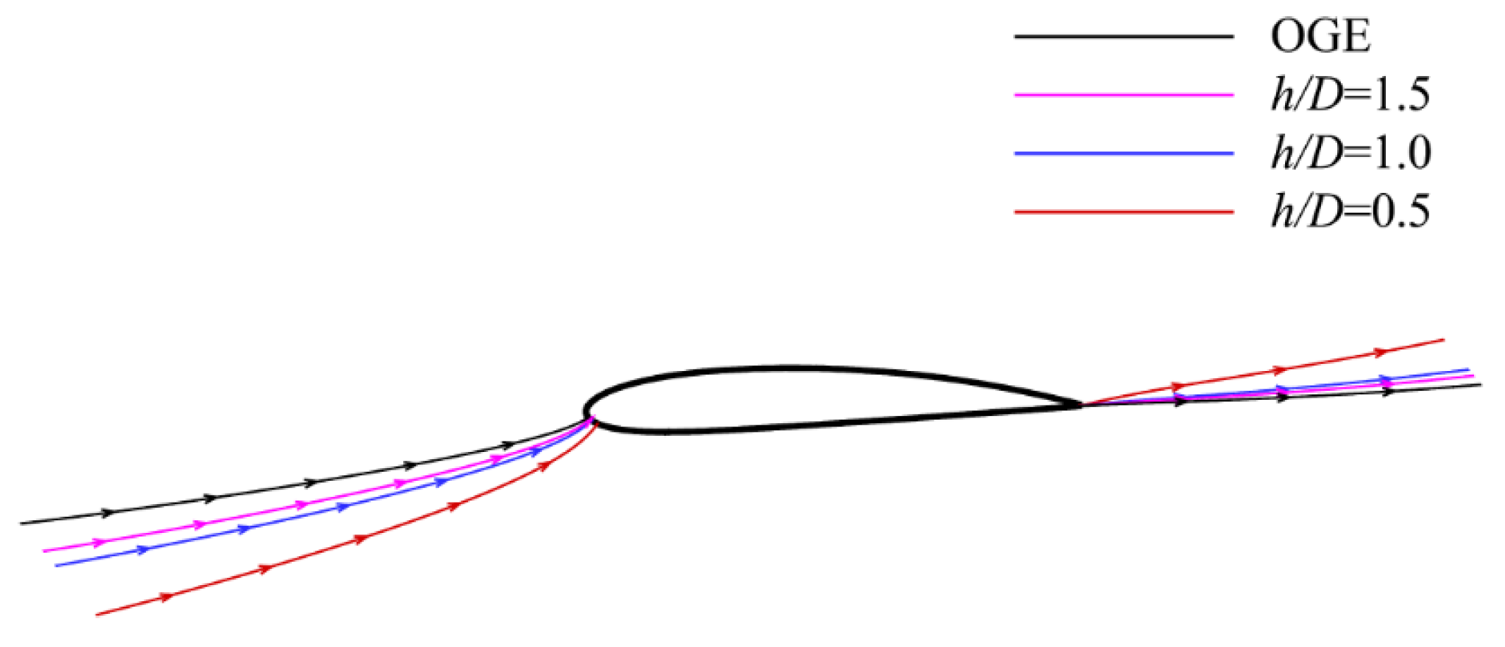
Figure 14 shows the stagnation streamlines of blade section at a three-quarter radius. It can be seen that when the ducted fan approaches the ground, the position of the leading-edge stagnation point moves backward along the pressure side of the airfoil. This indicates that the effective angle of attack of the incoming flow increases as the height decreases. According to the blade element theory [41] shown in Figure 15, the effective angle of attack of a blade element can be calculated by Equation (9). Some cross sections, as illustrated in Figure 16, are used to explore the flowfield. Figure 17 shows the azimuthally averaged axial velocity of the cross section in front of the blade. It should be noted that the velocities inside the boundary layers of the hub and duct inner surface are not plotted in Figure 17. As can be seen, when the ducted fan approaches the ground, Va decreases due to the increased blocking effect of the ground; Vt remains unchanged because the blade rotational speed does not change. Consequently, decreases and the effective angle of attack α increases according to Equation (9). As shown in Figure 17, Va is linearly distributed along the radial direction, with a larger value near the blade tip due to the acceleration effect of the duct lip on the airflow. Jimenez’s study [42] shows that an outboard-biased rotor inflow can improve the performance of a hovering ducted fan.
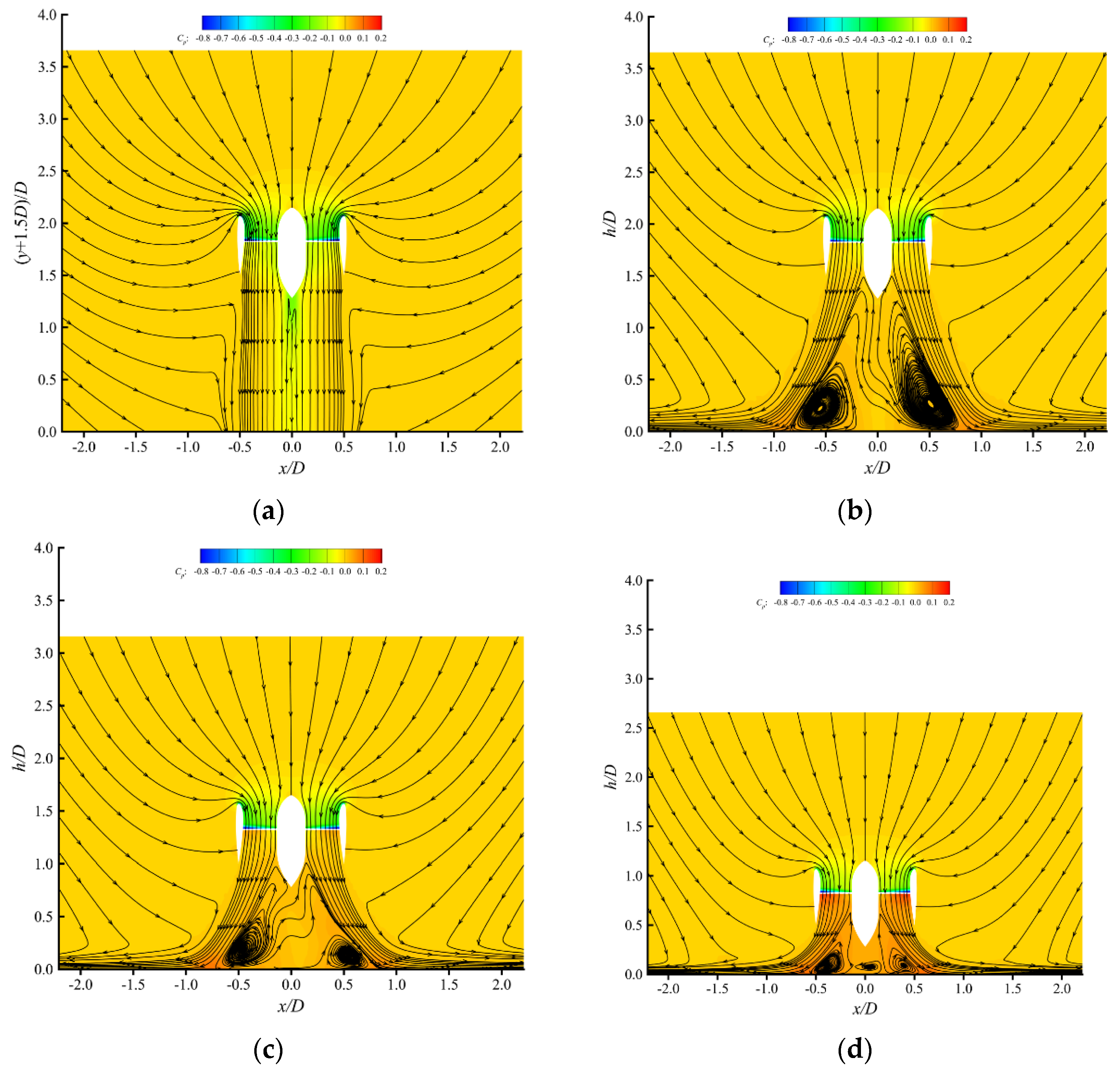
Figure 18 shows the pressure coefficient contours and streamlines on the cross section at Ψ = 0°–180°. It can be seen that the downward jet is blocked and spreads radially outward when the ducted fan gets close to the ground. Vortices are generated under the ducted fan due to the entrainment of the downward jet and the interaction between the downward jet and the airflow rebounding from the ground. When the height decreases to some degree, these vortices can induce secondary vortices, as shown in Figure 18d. The decelerated airflow forms a high-pressure zone between the blades and the ground, which leads to a considerable thrust increment in the blades. As the height decreases, the pressure in this zone increases, and thus the thrust of the blades increases as well.
The above analysis can be summarized as follows: when the ducted fan approaches the ground, the airflow through the duct is decelerated due to the blocking effect of the ground, and thus the static pressure of the airflow, hereafter referred to as ambient pressure, around the blades increases. The pressure on the suction and pressure sides of the blade generally shows an increasing trend. The decrease in the axial flow velocity in front of the blade increases the effective angle of attack of the blade, so that the pressure on the suction side of the blade tends to decrease and the pressure on the pressure side tends to increase. As a result, the pressure in the area near the leading edge of the suction side decreases, while the pressure in the other area increases. Consequently, it can be concluded that the increase in the blade thrust in ground effect is the result of the combined effect of the increase in the effective angle of attack and the increase in the ambient pressure.
3.3. Flow Physics Leading to Decrease in Duct Thrust
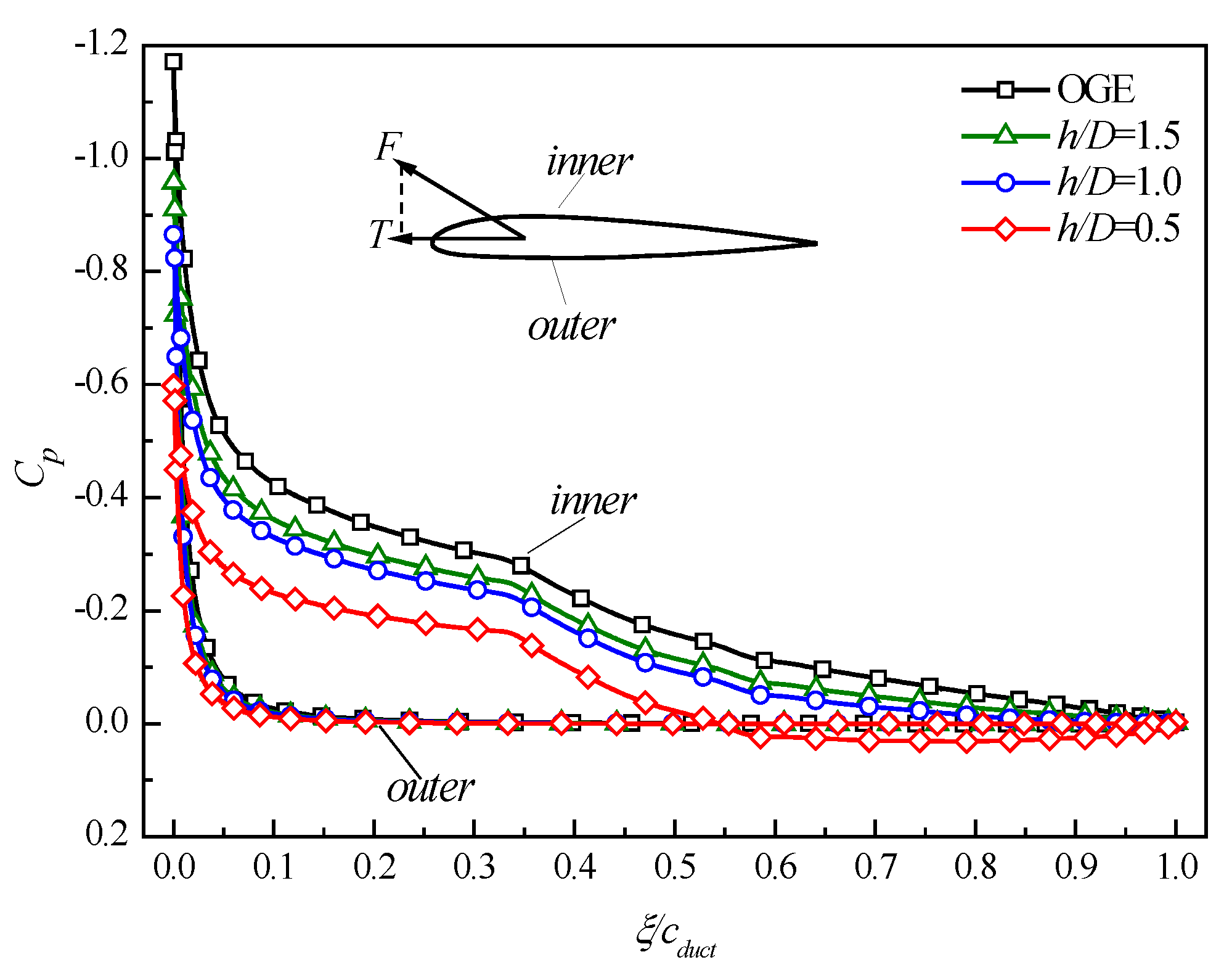
As can be seen in Figure 18, air is drawn into the duct and divided at a stagnation point on the outer surface near the trailing edge. The duct section acts like an airfoil and produces a resultant force vector that cants toward the duct lip. The axial component of this force vector provides additional thrust, as shown in Figure 19. When the ducted fan approaches the ground, the mass flow through the duct decreases, and the ambient pressure around the duct increases. The pressure increases on both the inner and outer surfaces of the duct, as shown in Figure 19. The change in the pressure on the outer surface is small, and the increase in pressure on the inner surface, especially near the lip, is the main reason for the reduction in duct thrust. The airflow ejected by the ducted fan deflects and forms a surface flow after hitting the ground. As the height decreases, the position where the deflection begins gets closer to the trailing edge of the duct, forcing the stagnation point to move upward along the outer surface of the duct, as shown in Figure 20. The outer side of the duct section is the pressure side of the airfoil, and the fact that the stagnation point moves forward along the pressure side of the airfoil indicates a decrease in the effective angle of attack. Based on the above analysis, the decrease in the duct thrust in the ground effect is the result of the combined effect of the following two effects: the increase in the ambient pressure caused by the decelerated airflow, and the decrease in the effective angle of attack caused by the deflection of the airflow.
4. Transitioning in Ground Effect
In this section, the aerodynamic characteristics of the ducted fan transitioning in the ground effect are studied, which may happen when a ducted fan UAV flies near the ground or when a ducted-fan-propelled V/STOL aircraft runs on the ground in STOL mode. A ducted fan is subjected to both crosswinds and the ground effect when transitioning in the ground effect. When conducting aerodynamic studies in the transition phase, the whole process is usually decomposed into several steady states at different angles of attack and advance ratios [8,9,10,21,27]. This approach is also adopted in this paper.
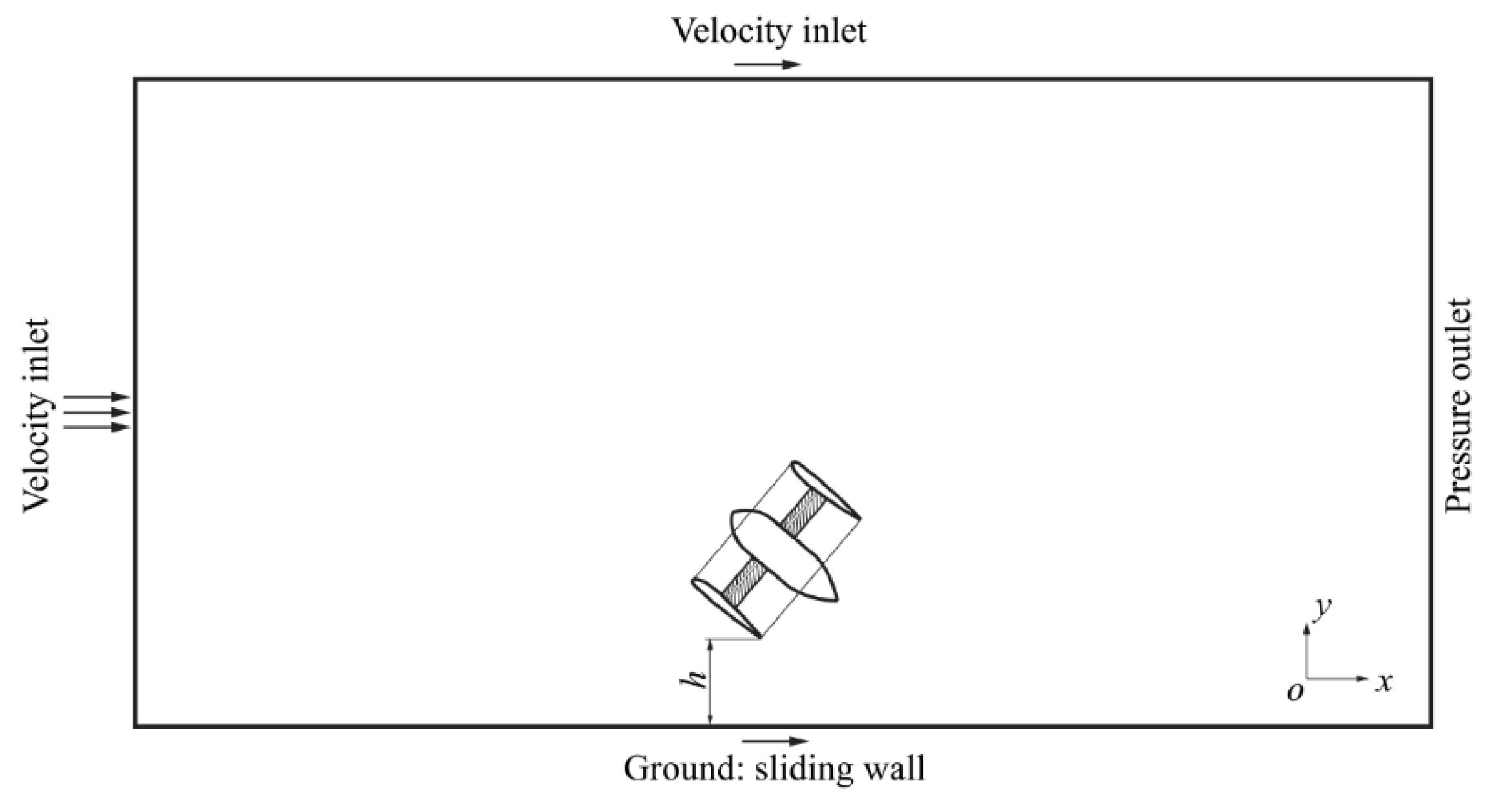
While performing the simulations of the ducted fan transition in the ground effect, the boundary conditions are shown in Figure 21: the bottom surface was set as a sliding wall with the same velocity as the freestream; the most downstream farfield boundary was set as the pressure outlet with a gauge pressure of 0 Pa relative to the reference pressure p∞; the other boundaries were set as velocity inlets. Three advance ratios were considered, that is, J = 0.1, 0.3, and 0.5, which cover a typical speed range during the transitional flight phase of a tilting ducted fan V/STOL aircraft [9]. The fan rotational speed was kept constant at 3500 rpm, and the advance ratios were adjusted by changing the freestream velocity. The Reynolds numbers based on the freestream velocity and duct length were Re = 1.0 × 10⁵, 3.1 × 10⁵, and 5.2 × 10⁵, respectively.
4.1. Ducted Fan Performance at Different Heights
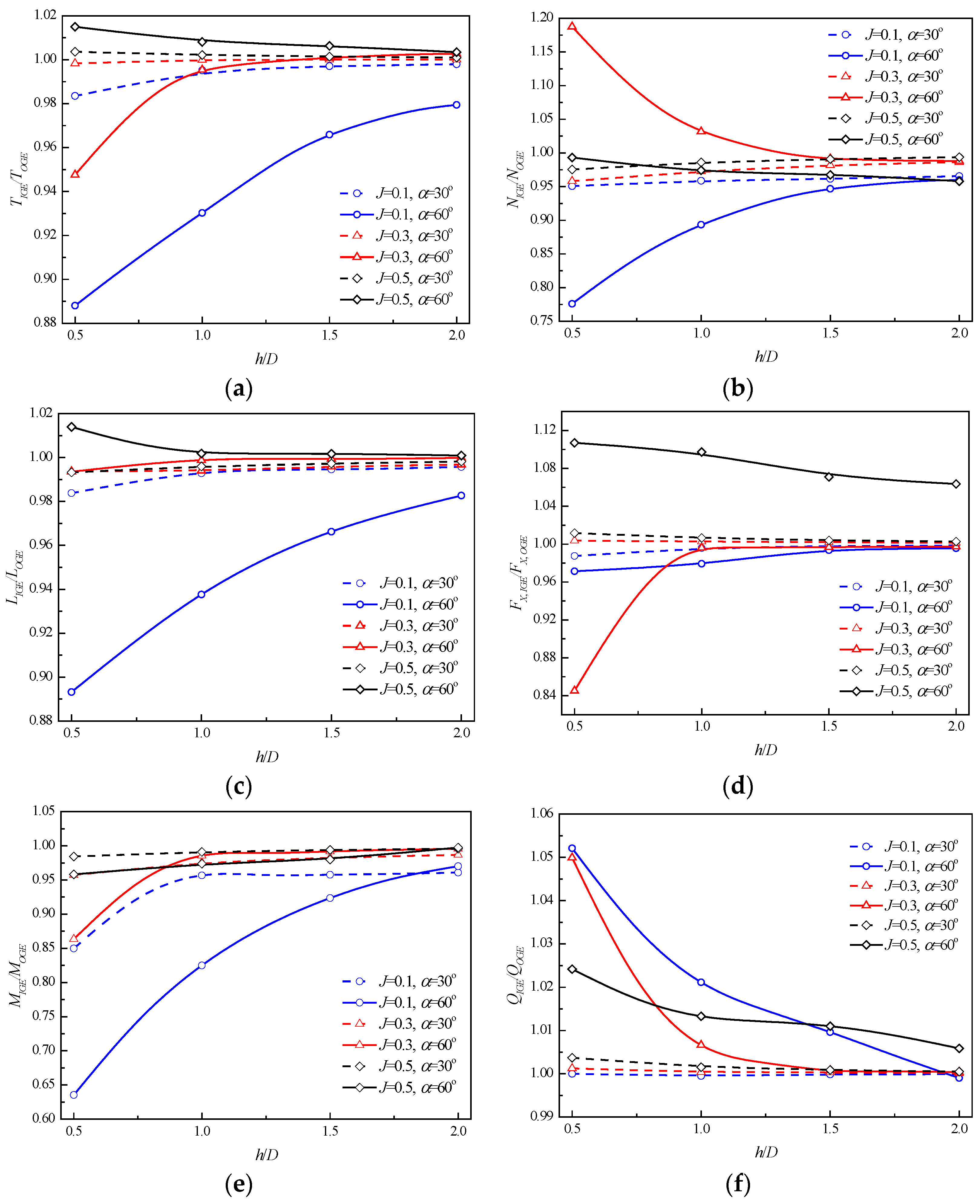
The aerodynamic performance of the ducted fan in the height range of 0.5D−2D was calculated with an interval of 0.5D at α = 30°, 60°. The results are shown in Figure 22. At α = 30°, the changes in thrust, normal force, lift, propulsive force, and torque at different heights are within 5%. Although the pitching moment of the duct has a maximum change of 15% at J = 0.1, the pitching moment as well as its influence is very small at J = 0.1, α = 30°. At α = 60°, the maximum changes in thrust, normal force, lift, propulsive force, and pitching moment are greater than 10%, and the maximum change in torque is 5.2%. The variation trends in the aerodynamic performance are different at different advance ratios at α = 60°. Taking the lift shown in Figure 22c as an example, as the height decreases, the lift decreases at J = 0.1, while the lift increases at J = 0.5. These indicate that the ground effect becomes stronger and more complex as the angle of attack increases. In general, the influence zone of the ground effect is reduced when there is a crosswind, and the ground effect becomes only significant when the height is less than 1D. Therefore, the height of 0.5D was selected in the subsequent analysis to further study the aerodynamic characteristics of the ducted fan transitioning in the ground effect.
4.2. Ducted Fan Performance at h/D = 0.5
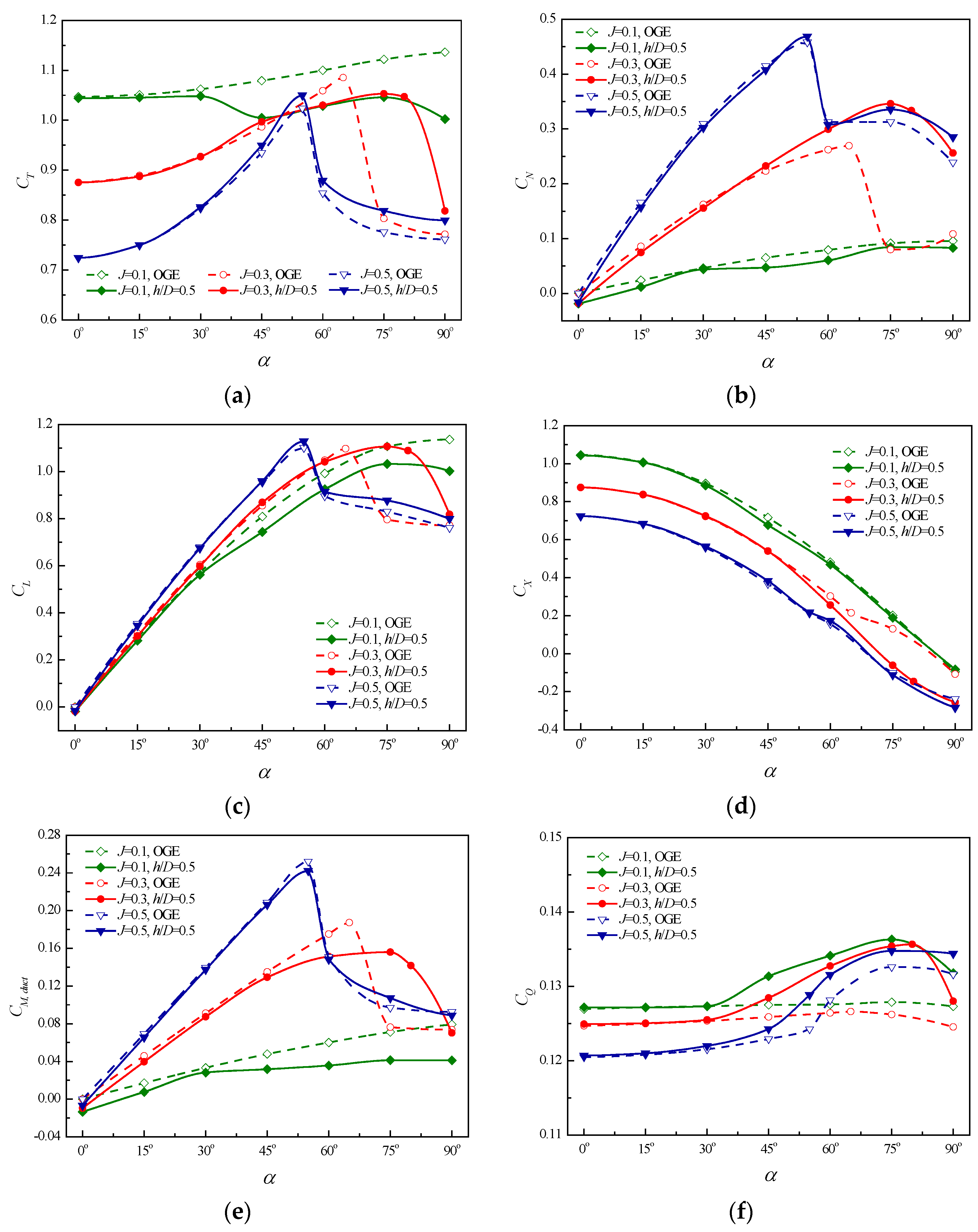
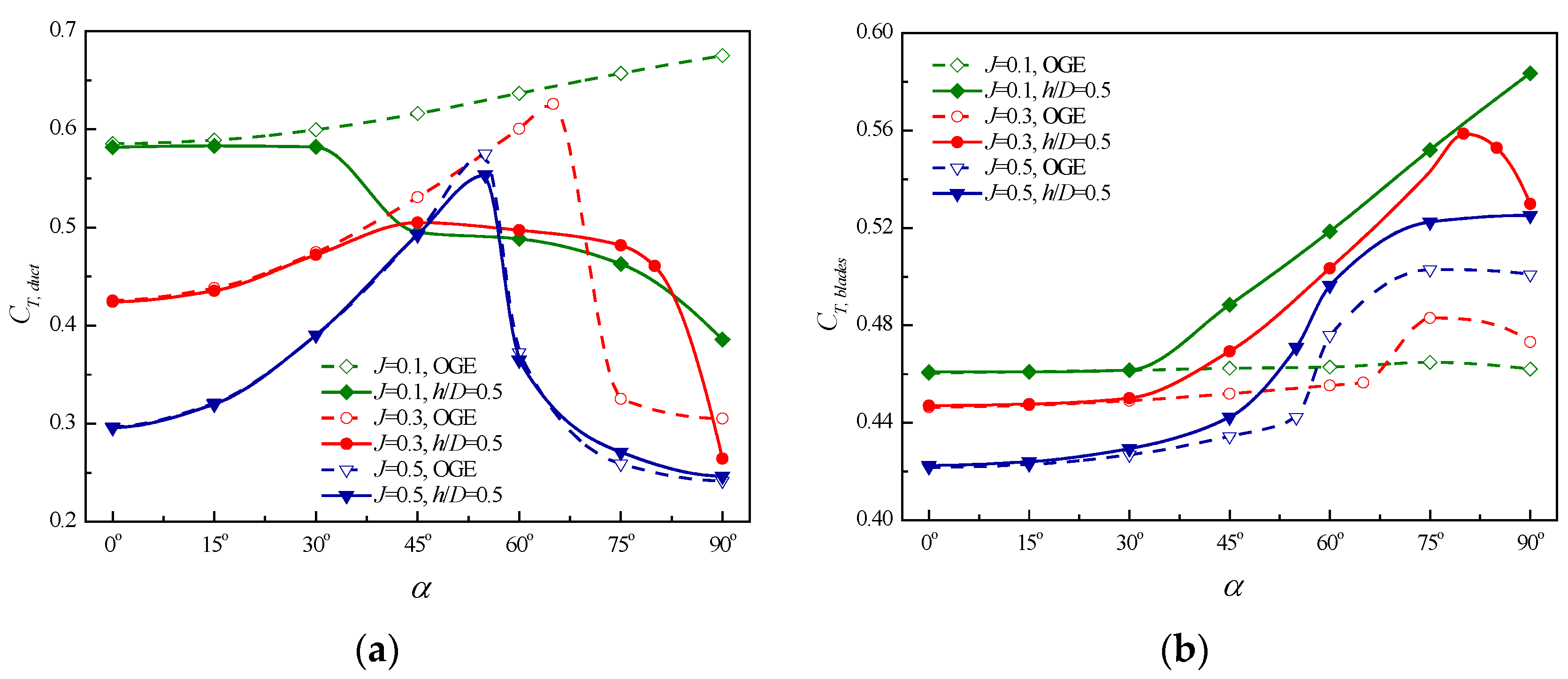
The aerodynamic performance of the ducted fan in the angle of attack range of 0°–90° at the height of 0.5D was calculated. The calculation interval was basically 15°, and the interval was changed to 5° near stall to determine the stall angle of attack accurately. The corresponding cases out of the ground effect were also calculated for comparison. The results are shown in Figure 23. The pitching moment of the blades is at least one order of magnitude smaller than that of the duct, so only the pitching moment coefficient of the duct is plotted. The variation trends of these coefficients are related, and thus the thrust coefficient is mainly analyzed. Figure 24 presents the division of thrust between the blades and the duct.
Stall occurs at a certain advance ratio and angle of attack, which is marked by a distinct reduction in the lift and pitching moment, as shown in Figure 22e and Figure 23c. The stall angle of attack is taken as the angle of attack when the lift coefficient of the ducted fan reaches a maximum, beyond which there is a significant drop in the lift coefficient. It should be noted that the ducted fan does not stall at this angle of attack. Hereafter, both the stall and stall angle of attack refer to those of the ducted fan. At J = 0.1, no stall occurs both in and out of the ground effect. At J = 0.3, the stall angle of attack increases from 65° out of the ground effect to 75° in the ground effect. At J = 0.5, the stall angle of attack is 55° both in and out of the ground effect. The stall is mainly caused by the flow separation on the windward side of the duct lip [8,9]. After the stall occurs, the duct thrust decreases and the blade thrust increases, as shown in Figure 24.
It can be seen from Figure 23 and Figure 24 that the ground effect is hardly detectable at angles of attack less than 30° even if the height off ground drops to 0.5D, especially at large advance ratios. Within this angle of attack range, the blade thrust remains almost constant at a specific advance ratio, and the variation in the ducted fan performance with the angle of attack is mainly caused by the duct.
At angles of attack greater than 30°, the blade thrust increases in the ground effect, and the increment magnitude decreases as the advance ratio increases, as shown in Figure 24b. At angles of attack greater than 30° before stall occurs, the blade thrust out of the ground effect remains almost constant, and the reason for the increase in blade thrust in the ground effect is similar to that in hovering. After stall occurs, the blade thrust out of the ground effect increases. This indicates that the increase in blade thrust after stall occurs in the ground effect is partly due to the stall. At high angles of attack, the duct thrust and total thrust show different variation trends at different advance ratios. In order to compare this with the hovering case, the case of α = 90° is taken for analysis. At J = 0.1, α = 90°, the duct thrust and total thrust decrease in the ground effect, which is the same as in the hovering case. At J = 0.3, α = 90°, although the duct thrust decreases in the ground effect as in the hovering case, the total thrust increases. At J = 0.5, α = 90°, both the duct thrust and the total thrust increase, which is different from the hovering case. In general, the aerodynamic performance of the ducted fan shows different variation trends at different advance ratios, and the aerodynamic problem becomes more complicated due to the crosswind.
4.3. Flow Physics Leading to Increase in Blade Thrust
Figure 25 shows the thrust coefficient of blades at different azimuths, where Ψ = 360° and Ψ = 0° are the same position. In Figure 25, Ψ = 270°–0°–90° is the windward side, and Ψ = 90°–180°–270° is the leeward side. At angles of attack less than 30°, the blade thrust changes little in the ground effect at all azimuthal positions; the difference in blade thrust at different azimuths is attributed to the different tangential velocity between the advancing and retreating blades. At angles of attack greater than 30° before stall occurs, the blades at different positions are affected by different degrees of ground effect, and thus, the magnitude of the thrust change is also different. After the stall occurs, the blades on the windward side are strongly affected by the separated flow, resulting in a different variation trend in blade thrust with azimuth compared with that before the stall.
After the stall occurs, the flow separation extends to the entire duct lip on the windward side. Taking the case of α = 90° as an example, Figure 26 shows the axial velocity contours on the cross sections passing through and intersecting the blade rotating plane. Negative values of the axial velocity indicate that the flow direction is locally reversed, as shown in the areas outside the black lines in Figure 26a and within the red dotted line in Figure 26b. The flow separation on the duct lip leads to a recirculation region across the rotor plane. When the blade rotates through this region, its outboard part will see an upwash resulting from the recirculation. The upwash increases the effective angle of attack of the blade locally, and thus, the blade produces more thrust in this region, as shown in Figure 25b. The intensity and scope of the recirculation increase in the ground effect compared with those out of the ground effect. Under the combined effect of the separated flow and ground effect, the thrust of the advancing blades may decrease compared with the value out of the ground effect, but the total thrust of the blades still increases. It should be noted that given the complexity of the flow and the limitations of the MRF-based method, the upwash may not be the only reason for the increase in blade thrust after the stall occurs.
4.4. Influence of Ground Vortex
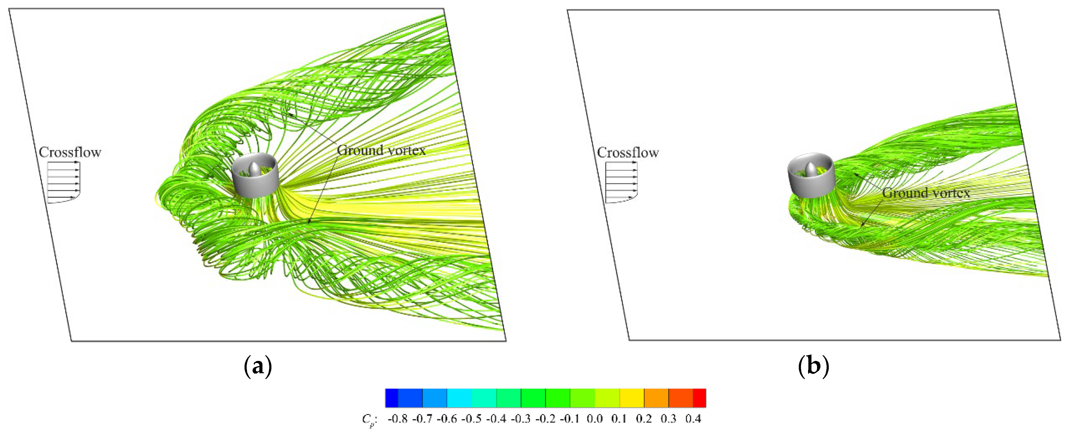
At high angles of attack, the radially spreading flow interacts with the crossflow after the jet impinges on the ground. As a consequence, two counter-rotating vortices trail away from the impinging zone and flow downstream. A ground vortex wrapped around the jet is formed in the shape of a horseshoe, as shown in Figure 27. The position and intensity of the ground vortex are related to the angle of attack and advance ratio. At the same angle of attack, as the advance ratio increases, the position of the ground vortex is further downstream, and the affected zone is much smaller.
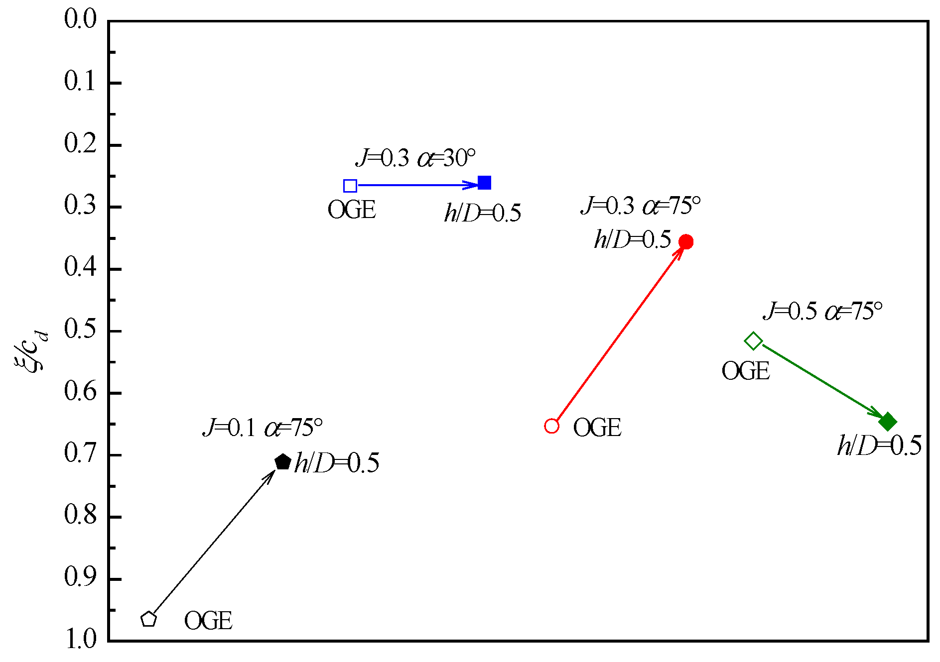
Figure 28 shows the pressure coefficient contours and streamlines on the symmetry plane under different freestream conditions, where the red dots are stagnation points. The chordwise relative positions of the stagnation point on the duct are shown in Figure 29. At small angles of attack, taking α = 30° as an example, the interaction between the oblique jet and the crossflow is weak, thus having little impact on the duct; the stagnation position only moves slightly forward, and the ducted fan performance remains almost unchanged. At high angles of attack, the center of the ground vortex is far away from the duct at J = 0.1, and its influence on the duct is also weak. The ducted fan is mainly affected by the ground effect similar to that in hovering near the ground, as analyzed in Section 3.1. At J = 0.3, the ground vortex is close to the outside of the duct. The upwash caused by the vortex leads to the stagnation point greatly moving forward and the effective angle of attack of the duct decreasing. Therefore, the duct thrust decreases and the stall angle of attack increases compared with those out of the ground effect. At J = 0.5, the ground vortex is close to the inner side of the duct. Its entrainment causes the stagnation point to move backward, increasing the effective angle of attack of the duct. Therefore, the duct thrust increases. It can be seen from the above analysis that the different positions and influence regions of the ground vortex contribute to the different variation trends of the ducted fan performance at different advance ratios. It should be noted that given the complexity of the flow and the limitations of the MRF-based method, the ground vortex may not be the only reason for the different variation trends in the ducted fan performance at different advance ratios.
5. Conclusions
Simulations of a ducted fan hovering and transitioning in the ground effect were performed by solving the RANS equations with the MRF approach and k-ε turbulence model. Through the analysis of the aerodynamic performance and flow physics of the ducted fan, the following conclusions are drawn:
- For the ducted fan studied in this paper, the ground effect is negligible in hovering when the height off the ground is greater than 3D and becomes significant when the height is less than 1.5D. As the height decreases, the thrust of the blades increases, while the thrust of the duct decreases. Compared with the values out of the ground effect, at the height of 0.5D, the blade thrust increases by 28.4%, and the duct thrust decreases by 41.1%, resulting in a total thrust decrease by 12.5%; the power loading decreases by 14.6%. The efficiency of the ducted fan decreases in the ground effect.
- When the ducted fan hovers in the ground effect, the increase in the blade thrust is the result of the combined effect of the increase in the effective angle of attack of the blade and the increase in the ambient pressure; the decrease in the duct thrust is the result of the combined effect of the decrease in the effective angle of attack of the duct and the increase in the ambient pressure.
- Stall occurs at a certain advance ratio and angle of attack when transitioning in the ground effect. The ground effect delays the occurrence of stall at some advance ratios. After stall occurs, the upwash resulting from the separated flow on the duct lip causes an increase in the total thrust of the blades.
- When the advance ratio is greater than 0.1, the influence zone of the ground effect is reduced, and the ground effect is hardly detectable at angles of attack less than 30° even if the height drops to 0.5D. At the height of 0.5D and high angles of attack, after the jet impinges on the ground, the interaction between the radially spreading wall flow and the crossflow generates ground vortices. The different positions and influence regions of the ground vortex at different advance ratios contribute to the different variation trends of the ducted fan performance and make the aerodynamic problem more complicated.
Author Contributions
Conceptualization, Y.T. and Z.W.; formal analysis, Y.Z.; investigation, Y.T. and Z.W.; methodology, Y.Z. and Y.T.; writing—original draft, Y.Z.; writing—review and editing, Y.T. and Z.W. All authors have read and agreed to the published version of the manuscript.
Funding
This research received no external funding.
Institutional Review Board Statement
Not applicable.
Informed Consent Statement
Not applicable.
Data Availability Statement
Not applicable.
Conflicts of Interest
The authors declare no conflict of interest.
Nomenclature
| Symbols | Definition |
| r | Radial distance from fan axis |
| Rb | Blade radius |
| Db | Blade diameter |
| D | Duct exit diameter |
| cd | Duct chord |
| α | Angle of attack |
| V∞ | Freestream velocity |
| T | Thrust |
| N | Normal force |
| L | Lift |
| FX | Propulsive force |
| M | Pitching moment |
| Q | Blade torque |
| n | Fan rotational speed, revolution/s |
| ω | Fan rotational speed, revolution/min |
| Ω | Fan rotational speed, radian/s |
| ρ | Air density, 1.225 kg/m3 |
| p | Static pressure |
| p∞ | Static pressure of freestream, 101325 Pa |
| Vtip | Blade tip velocity, ΩRb |
| y+ | Nondimensional wall distance of the first mesh layer |
| h | Distance from the lowest point of duct trailing edge to the ground |
| P | Shaft power, 2πQn |
| PL | Power loading, T/P, |
| Nondimensional chordwise distance from blade leading edge | |
| θ | Pitch angle of blade section |
| Inflow angle | |
| Va | Induced velocity parallel to fan axis |
| Vt | Tangential velocity of blade element, Ωr |
| ξ | Chordwise distance from duct leading edge |
| Rlocal | Radius of duct inner surface |
| Ψ | Azimuth angle |
References
- Black, D.M.; Wainauski, H.S.; Rohrbach, C. Shrouded Propellers–A Comprehensive Performance Study. In Proceedings of the AIAA 5th Annual Meeting and Technical Display, Philadelphia, PA, USA, 21–24 October 1968. [Google Scholar] [CrossRef]
- Anderson, S.B. Historical Overview of V/STOL Aircraft Technology; Report No.: NASA-TM-812801; National Aeronautics and Space Administration: Washington, DC, USA, 1981.
- Paxhia, V.B.; Sing, E.Y. X-22A Design Development. J. Aircr. 1965, 2, 2–8. [Google Scholar] [CrossRef]
- BELL NEXUS. Available online: https://www.bellflight.com/products/bell-nexus (accessed on 12 July 2022).
- Architectural Performance Assessment of an Electric Vertical Take-off and Landing (e-VTOL) Aircraft Based on a Ducted Vectored Thrust Concept. Available online: https://lilium.com/files/redaktion/refresh_feb2021/investors/Lilium_7-Seater_Paper.pdf (accessed on 12 July 2022).
- Whiteside, S.; Pollard, B. Conceptual Design of a Tiltduct Reference Vehicle for Urban Air Mobility. In Proceedings of the VFS Aeromechanics for Advanced Vertical Flight Technical Meeting, San Jose, CA, USA, 25–27 January 2022. [Google Scholar]
- Sacks, A.H.; Burnell, J.A. Ducted propellers—A critical review of the state of the art. Prog. Aeosp. Sci. 1962, 3, 85–135. [Google Scholar] [CrossRef]
- Mort, K.W.; Yaggy, P.F. Aerodynamic Characteristics of a 4-Foot-Diameter Ducted Fan Mounted on the Tip of a Semispan Wing; Report No.: NASA TN D-1301; National Aeronautics and Space Administration: Washington, DC, USA, 1962.
- Grunwald, K.J.; Goodson, K.W. Aerodynamic Loads on an Isolated Shrouded-Propeller Configuration of Angles of Attack from −10° to 110°; Report No.: NASA TN D-995; National Aeronautics and Space Administration: Washington, DC, USA, 1962.
- Mort, K.W.; Gamse, B. A Wind-Tunnel Investigation of a 7-Foot-Diameter Ducted Propeller; Report No.: NASA TN D-4142; National Aeronautics and Space Administration: Washington, DC, USA, 1967.
- Abrego, A.I.; Bulaga, R.W.; Rutkowski, M.Y. Performance Study of a Ducted Fan System. In Proceedings of the American Helicopter Society Aerodynamics, Acoustics and Test and Evaluation Technical Specialists Meeting, San Francisco, CA, USA, 23–25 January 2002. [Google Scholar]
- Martin, P.; Tung, C. Performance and Flowfield Measurements on a 10-Inch Ducted Rotor VTOL UAV. In Proceedings of the 60th American Helicopter Society Annual Forum, Baltimore, MD, USA, 7–10 June 2004. [Google Scholar]
- Lind, R.; Nathman, J.; Gilchrist, I. Ducted Rotor Performance Calculations and Comparison with Experimental Data. In Proceedings of the 44th AIAA Aerospace Sciences Meeting and Exhibit, Reno, NV, USA, 9–12 January 2006. [Google Scholar] [CrossRef]
- Graf, W.; Fleming, J.; Ng, W. Improving Ducted Fan UAV Aerodynamics in Forward Flight. In Proceedings of the 46th AIAA Aerospace Sciences Meeting and Exhibit, Reno, NV, USA, 7–10 January 2008. [Google Scholar] [CrossRef]
- Pereira, J.L. Hover and Wind-Tunnel Testing of Shrouded Rotors for Improved Micro Air Vehicle Design. Ph.D. Thesis, University of Maryland, College Park, MD, USA, 2008. [Google Scholar]
- Colman, M.; Suzuki, S.; Kubo, D. Wind Tunnel Test Results and Performance Prediction For a Ducted Fan with Collective and Cyclic Pitch Actuation for VTOL with Efficient Cruise. In Proceedings of the AIAA Atmospheric Flight Mechanics Conference, Portland, OR, USA, 8–11 August 2011. [Google Scholar] [CrossRef]
- Hrishikeshavan, V.; Chopra, I. Performance, Flight Testing of a Shrouded Rotor Micro Air Vehicle in Edgewise Gusts. J. Aircr. 2012, 49, 193–205. [Google Scholar] [CrossRef]
- Ohanian, O.J., III; Gelhausen, P.A.; Inman, D.J. Nondimensional Modeling of Ducted-Fan Aerodynamics. J. Aircr. 2012, 49, 126–140. [Google Scholar] [CrossRef]
- Cai, H.; Wu, Z.; Deng, S.; Xiao, T. Numerical Prediction of Unsteady Aerodynamics for A Ducted Fan Micro Air Vehicle. Proc. Inst. Mech. Eng. Part G J. Aerosp. Eng. 2012, 229, 87–95. [Google Scholar] [CrossRef]
- Ryu, M.; Cho, L.; Cho, J. Aerodynamic Analysis of the Ducted Fan for a VTOL UAV in Crosswinds. Trans. Jpn. Soc. Aeronaut. Space Sci. 2016, 59, 47–55. [Google Scholar] [CrossRef] [Green Version]
- Raeisi, B.; Alighanbari, H. Simulation and Analysis of Flow around Tilting Asymmetric Ducted Fans Mounted at the Wing Tips of a Vertical Take-Off and Landing Unmanned Aerial Vehicle. Proc. Inst. Mech. Eng. Part G J. Aerosp. Eng. 2018, 232, 2870–2897. [Google Scholar] [CrossRef]
- Raeisi, B.; Alighanbari, H. Effects of Tilting Rate Variations on the Aerodynamics of The Tilting Ducted Fans Mounted At The Wing Tips Of A Vertical Take-Off And Landing Unmanned Aerial Vehicle. Proc. Inst. Mech. Eng. Part G J. Aerosp. Eng. 2018, 232, 1803–1813. [Google Scholar] [CrossRef]
- Misiorowski, M.P.; Gandhi, F.S.; Oberai, A.A. Computational analysis and flow physics of a ducted rotor in edgewise flight. J. Am. Helicopter Soc. 2019, 64, 1–14. [Google Scholar] [CrossRef]
- Deng, S.; Wang, S.; Zhang, Z. Aerodynamic Performance Assessment of a Ducted Fan UAV for VTOL Applications. Aerosp. Sci. Technol. 2020, 103, 105895. [Google Scholar] [CrossRef]
- Akturk, A.; Camci, C. Double-Ducted Fan as an Effective Lip Separation Control Concept for Vertical-Takeoff-and-Landing Vehicles. J. Aircr. 2022, 59, 233–252. [Google Scholar] [CrossRef]
- Zhang, T.; Barakos, G.N. Review on Ducted Fans for Compound Rotorcraft. Aeronaut. J. 2020, 124, 941–974. [Google Scholar] [CrossRef]
- Giullianetti, D.J.; Biggers, J.C.; Maki, R.L. Longitudinal Aerodynamic Characteristics in Ground Effect of a Large-Scale, V/STOL Model with Four Tilting Ducted Fans Arranged in a Dual Tandem Configuration; Report No.: NASA TN D-4218; National Aeronautics and Space Administration: Washington, DC, USA, 1967.
- De Divitiis, N. Performance and Stability Analysis of a Shrouded-Fan Unmanned Aerial Vehicle. J. Aircr. 2006, 43, 681–691. [Google Scholar] [CrossRef]
- Hosseini, Z.; Ramirez-Serrano, A.; Martinuzzi, R.J. Ground/Wall Effects on a Tilting Ducted Fan. Int. J. Micro Air Veh. 2011, 3, 119–141. [Google Scholar] [CrossRef]
- Ai, T.; Xu, B.; Xiang, C.; Fan, W.; Zhang, Y. Aerodynamic Analysis and Control for a Novel Coaxial Ducted Fan Aerial Robot in Ground Effect. Int. J. Adv. Robot Syst. 2020, 17, 1–15. [Google Scholar] [CrossRef]
- Gourdain, N.; Singh, D.; Jardin, T.; Prothin, S. Analysis of the Turbulent Wake Generated by a Micro Air Vehicle Hovering near the Ground with a Lattice Boltzmann Method. J. Am. Helicopter Soc. 2017, 62, 1–12. [Google Scholar] [CrossRef]
- Deng, S.; Ren, Z. Experimental Study of a Ducted Contra-Rotating Lift Fan for Vertical/Short Takeoff and Landing Unmanned Aerial Vehicle Application. Proc. Inst. Mech. Eng. Part G J. Aerosp. Eng. 2018, 232, 3108–3117. [Google Scholar] [CrossRef]
- Deng, Y. Experimental Investigation on Ground Effect of Ducted Fan System for VTOL UAV. In Proceedings of the 2018 Asia-Pacific International Symposium on Aerospace Technology, Chengdu, China, 16–18 October 2018. [Google Scholar] [CrossRef]
- Han, H.; Xiang, C.; Xu, B.; Yu, Y. Aerodynamic Performance and Analysis of a Hovering Micro-Scale Shrouded Rotor in Confined Environment. Adv. Mech. Eng. 2019, 11, 1–21. [Google Scholar] [CrossRef]
- Jin, Y.; Fu, Y.; Qian, Y.; Zhang, Y. A Moore-Greitzer Model for Ducted Fans in Ground Effect. J. Appl. Fluid Mech. 2020, 13, 693–701. [Google Scholar] [CrossRef]
- Han, H.; Xiang, C.; Xu, B.; Yu, Y. Experimental and Computational Investigation on Comparison of Micro-Scale Open Rotor and Shrouded Rotor Hovering in Ground Effect. Proc. Inst. Mech. Eng. Part G J. Aerosp. Eng. 2021, 235, 553–565. [Google Scholar] [CrossRef]
- Mi, B. Numerical Investigation on Aerodynamic Performance of a Ducted Fan under Interferences from the Ground, Static Water and Dynamic Waves. Aerosp. Sci. Technol. 2020, 100, 105821. [Google Scholar] [CrossRef]
- Siemens Industries Digital Software. Simcenter STAR-CCM+ User Guide, version 2020.1; Siemens Industries Digital Software: Munich, Germany, 2020. [Google Scholar]
- Bunker, R.S. Axial turbine blade tips: Function, design, and durability. J. Propuls. Power 2006, 22, 271–285. [Google Scholar] [CrossRef]
- Qing, J.; Hu, Y.; Wang, Y.; Liu, Z.; Fu, X.; Liu, W. Kriging Assisted Integrated Rotor-Duct Optimization for Ducted Fan in Hover. In Proceedings of the AIAA Scitech 2019 Forum, San Diego, CA, USA, 7–11 January 2019. [Google Scholar] [CrossRef]
- Leishman, G.J. Principles of Helicopter Aerodynamics, 2nd ed.; Cambridge University Press: New York, NY, USA, 2006; pp. 117–124. [Google Scholar]
- Jimenez, B.G.; Singh, R. Effect of Duct-Rotor Aerodynamic Interactions on Blade Design for Hover and Axial Flight. In Proceedings of the 53rd AIAA Aerospace Sciences Meeting, Kissimmee, FL, USA, 5–9 January 2015. [Google Scholar] [CrossRef]
Figure 1.
Ducted fan model.

Figure 2.
Blade chord and twist distributions.
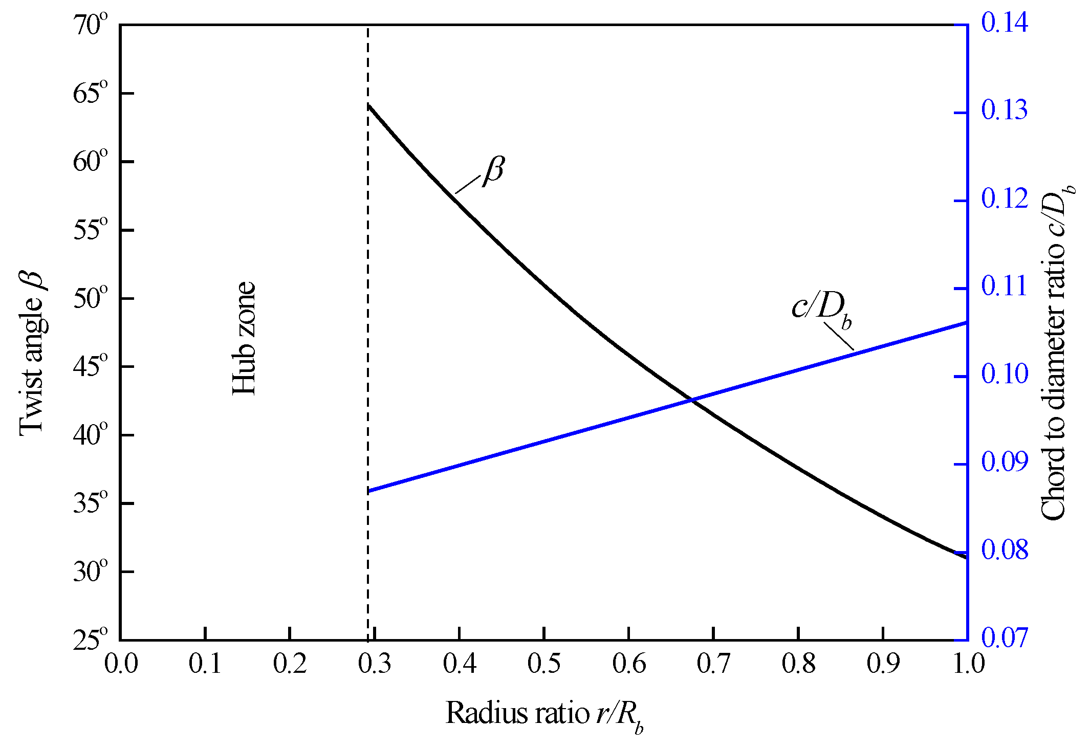
Figure 3.
Coordinate system, showing positive sense of velocity, angle of attack, forces, and moments.
Figure 3.
Coordinate system, showing positive sense of velocity, angle of attack, forces, and moments.
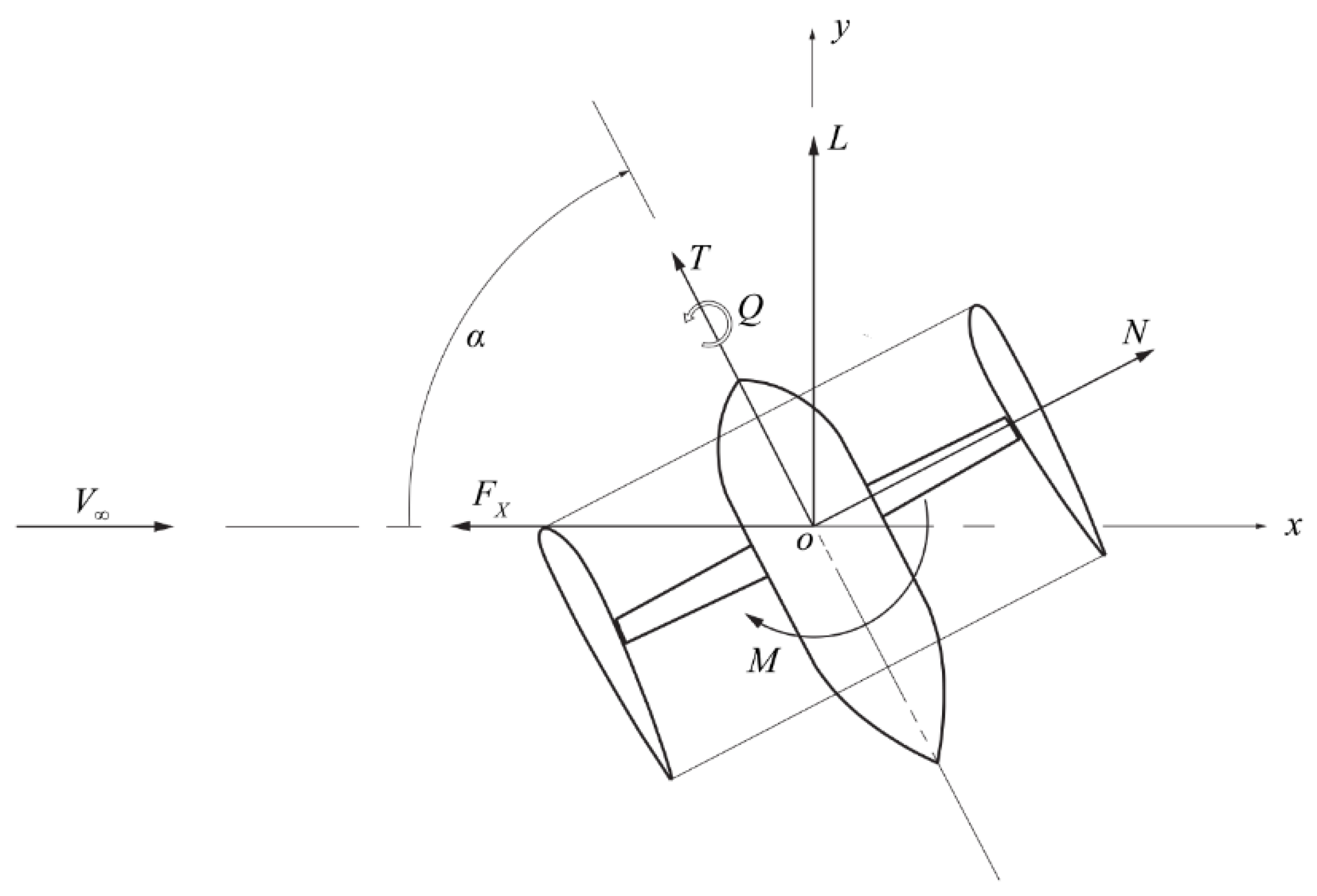
Figure 4.
Computational domain and boundary conditions when out of ground effect: (a) boundary conditions; (b) computational domain divisions.
Figure 4.
Computational domain and boundary conditions when out of ground effect: (a) boundary conditions; (b) computational domain divisions.
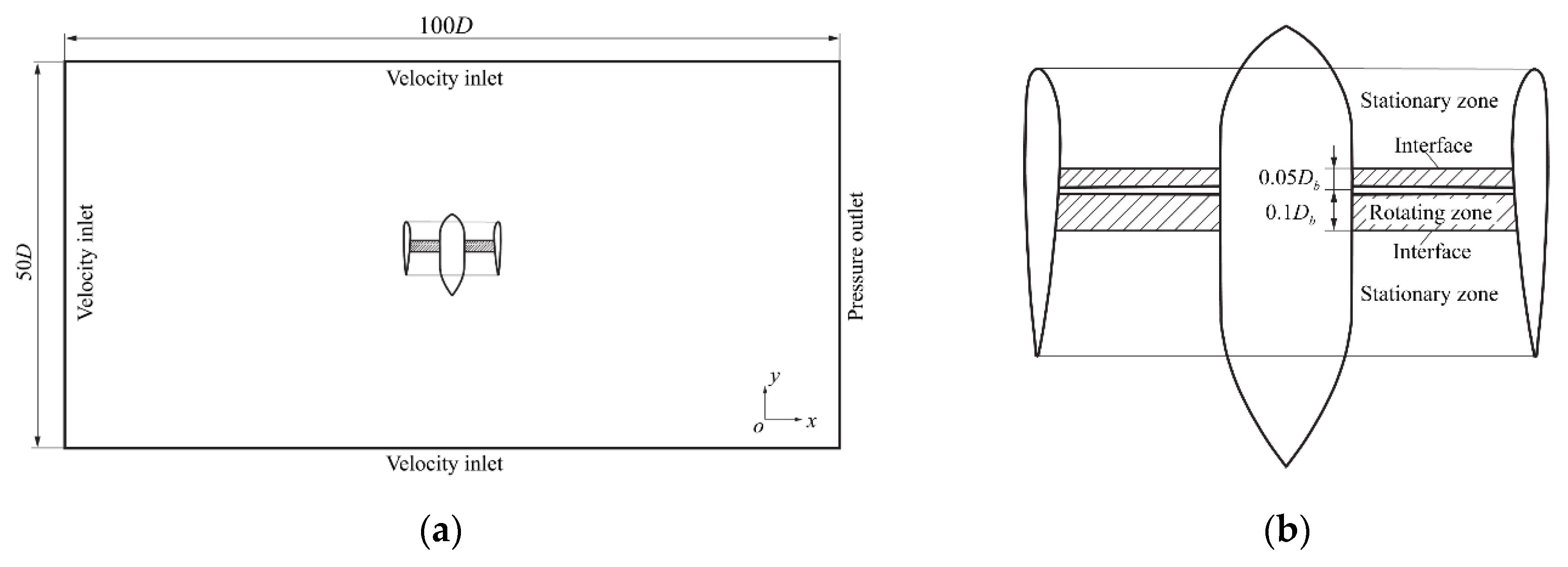
Figure 5.
Comparison of results obtained with pressure inlet and velocity inlet boundary conditions: (a) force coefficients; (b) continuity residuals.
Figure 5.
Comparison of results obtained with pressure inlet and velocity inlet boundary conditions: (a) force coefficients; (b) continuity residuals.
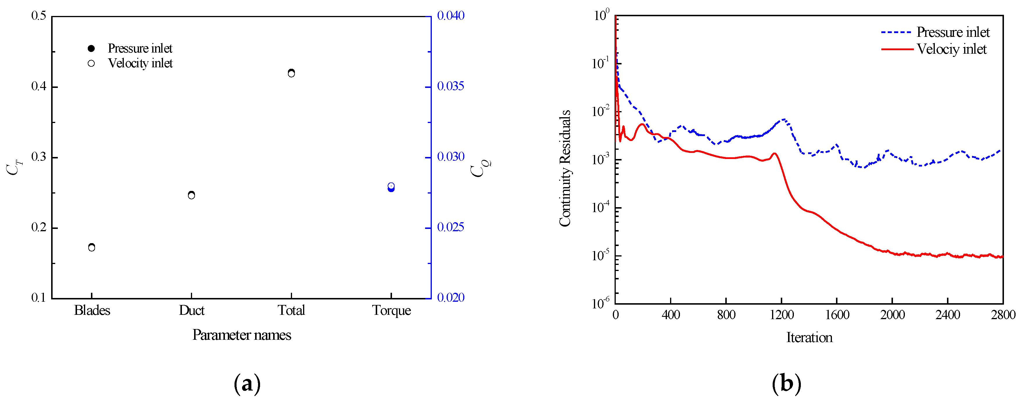
Figure 6.
Coefficients calculated by different grid densities, Grunwald’s model in hovering.
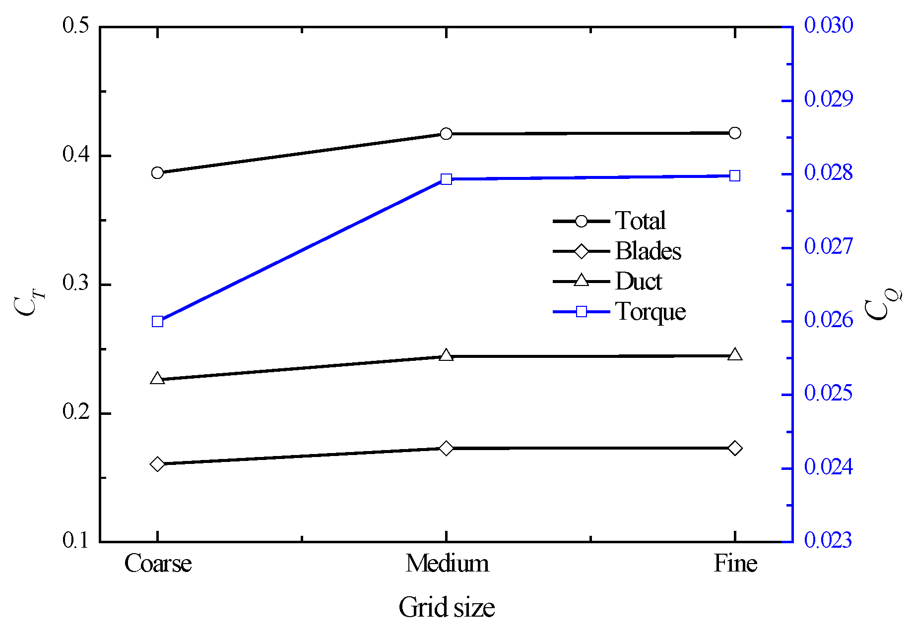
Figure 7.
Comparison of streamlines obtained via sliding mesh method and MRF method, with pressure coefficients contour as background: (a) limiting streamlines on suction side of blade; (b) streamlines on cross section at r/Rb = 0.99.
Figure 7.
Comparison of streamlines obtained via sliding mesh method and MRF method, with pressure coefficients contour as background: (a) limiting streamlines on suction side of blade; (b) streamlines on cross section at r/Rb = 0.99.

Figure 8.
The medium mesh used in simulations: (a) surface mesh on blade and duct; (b) cross section mesh around blade.
Figure 8.
The medium mesh used in simulations: (a) surface mesh on blade and duct; (b) cross section mesh around blade.

Figure 9.
Boundary conditions when hovering in ground effect.

Figure 10.
Coefficients calculated by different grid densities; ducted fan studied in this paper: (a) hovering out of ground effect; (b) hovering in ground effect.
Figure 10.
Coefficients calculated by different grid densities; ducted fan studied in this paper: (a) hovering out of ground effect; (b) hovering in ground effect.

Figure 11.
Variation in ducted fan performance with height: (a) thrust ratios; (b) torque and power loading ratios.
Figure 11.
Variation in ducted fan performance with height: (a) thrust ratios; (b) torque and power loading ratios.

Figure 12.
Pressure coefficient contours on blade surfaces at different heights: (a) OGE; (b) h/D = 1.5; (c) h/D = 1.0; (d) h/D = 0.5.
Figure 12.
Pressure coefficient contours on blade surfaces at different heights: (a) OGE; (b) h/D = 1.5; (c) h/D = 1.0; (d) h/D = 0.5.

Figure 13.
Chordwise pressure coefficient distribution at different radial locations: (a) r/Rb = 0.35; (b) r/Rb = 0.55; (c) r/Rb = 0.75; (d) r/Rb = 0.95.
Figure 13.
Chordwise pressure coefficient distribution at different radial locations: (a) r/Rb = 0.35; (b) r/Rb = 0.55; (c) r/Rb = 0.75; (d) r/Rb = 0.95.

Figure 14.
Stagnation streamlines of blade section at three-quarter radius.

Figure 15.
Flow environment at a typical blade element.
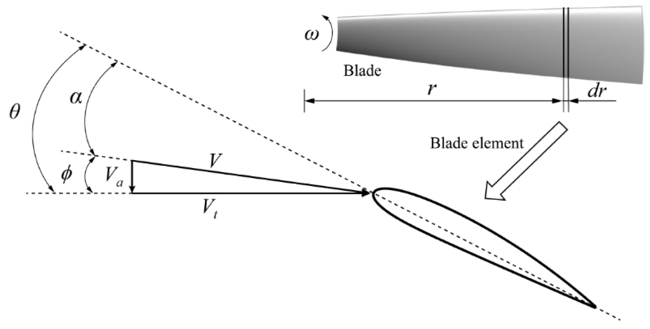
Figure 16.
Locations of cross sections used in analysis: (a) azimuthal cross sections; (b) axial cross sections.
Figure 16.
Locations of cross sections used in analysis: (a) azimuthal cross sections; (b) axial cross sections.

Figure 17.
Radial distribution of azimuthally averaged axial velocity on cross section at ξ/cd=0.39.
Figure 17.
Radial distribution of azimuthally averaged axial velocity on cross section at ξ/cd=0.39.
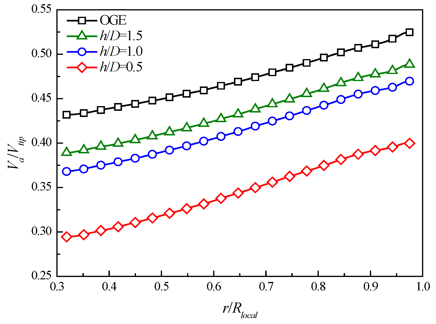
Figure 18.
Pressure coefficient contour and streamlines on cross section at Ψ = 0°−180°: (a) OGE; (b) h/D = 1.5; (c) h/D = 1.0; (d) h/D = 0.5.
Figure 18.
Pressure coefficient contour and streamlines on cross section at Ψ = 0°−180°: (a) OGE; (b) h/D = 1.5; (c) h/D = 1.0; (d) h/D = 0.5.

Figure 19.
Pressure coefficient distributions on duct section at Ψ = 22.5°.

Figure 20.
Stagnation streamlines of duct section at Ψ = 22.5°.
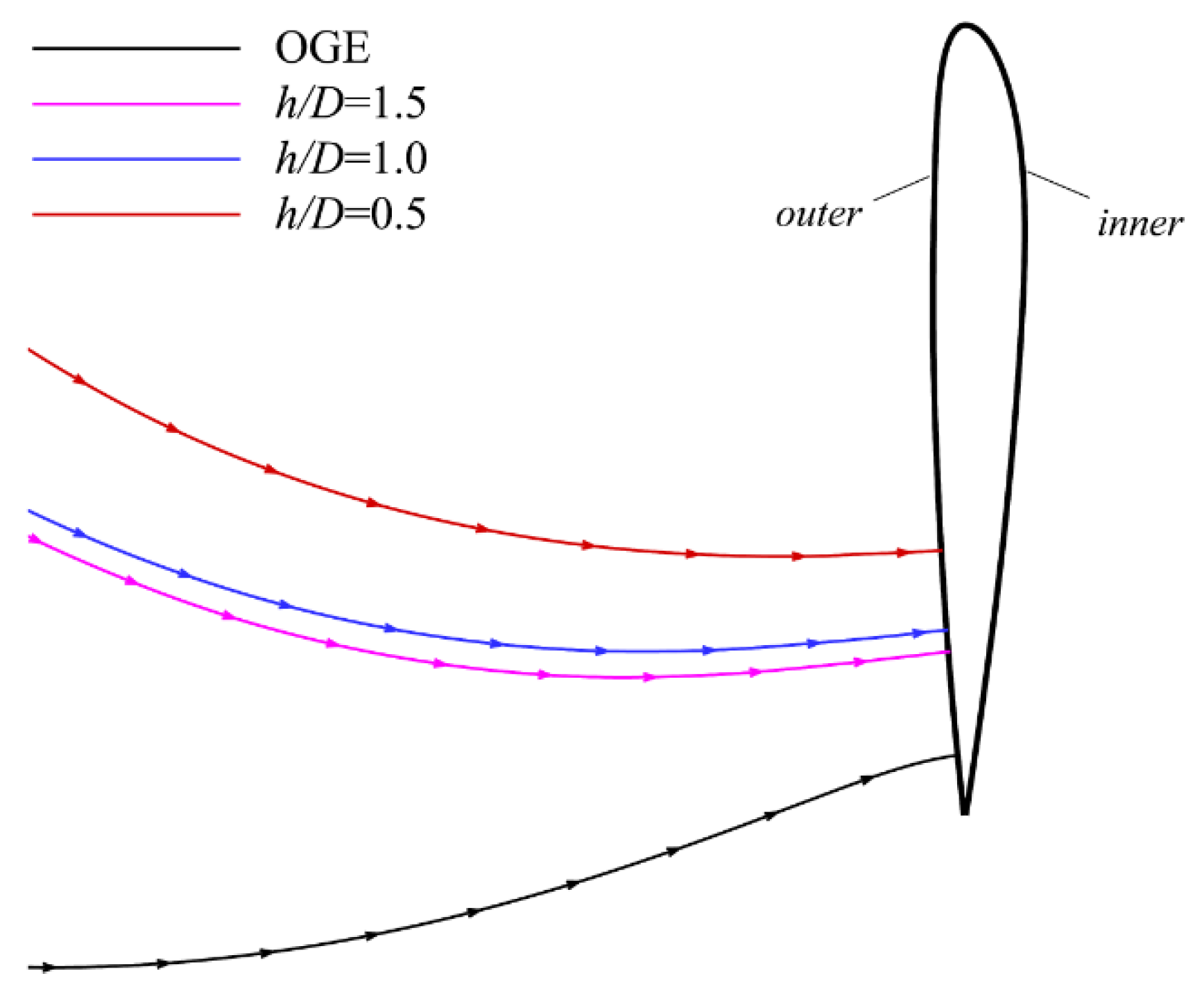
Figure 21.
Boundary conditions when transitioning in ground effect.

Figure 22.
Load ratios at different heights, advance ratios, and angles of attack: (a) thrust ratio; (b) normal force ratio; (c) lift ratio; (d) propulsive force ratio; (e) duct pitching moment ratio; (f) torque ratio.
Figure 22.
Load ratios at different heights, advance ratios, and angles of attack: (a) thrust ratio; (b) normal force ratio; (c) lift ratio; (d) propulsive force ratio; (e) duct pitching moment ratio; (f) torque ratio.

Figure 23.
Aerodynamic coefficients at different advance ratios and angles of attack: (a) thrust coefficient; (b) normal force coefficient; (c) lift coefficient; (d) propulsive force coefficient; (e) pitching moment coefficient of duct; (f) torque coefficient.
Figure 23.
Aerodynamic coefficients at different advance ratios and angles of attack: (a) thrust coefficient; (b) normal force coefficient; (c) lift coefficient; (d) propulsive force coefficient; (e) pitching moment coefficient of duct; (f) torque coefficient.

Figure 24.
Division of thrust between the blades and the duct: (a) thrust coefficient of duct; (b) thrust coefficient of blades.
Figure 24.
Division of thrust between the blades and the duct: (a) thrust coefficient of duct; (b) thrust coefficient of blades.

Figure 25.
Thrust coefficient of blades at different azimuths at J = 0.5: (a) before stall; (b) after stall.
Figure 25.
Thrust coefficient of blades at different azimuths at J = 0.5: (a) before stall; (b) after stall.
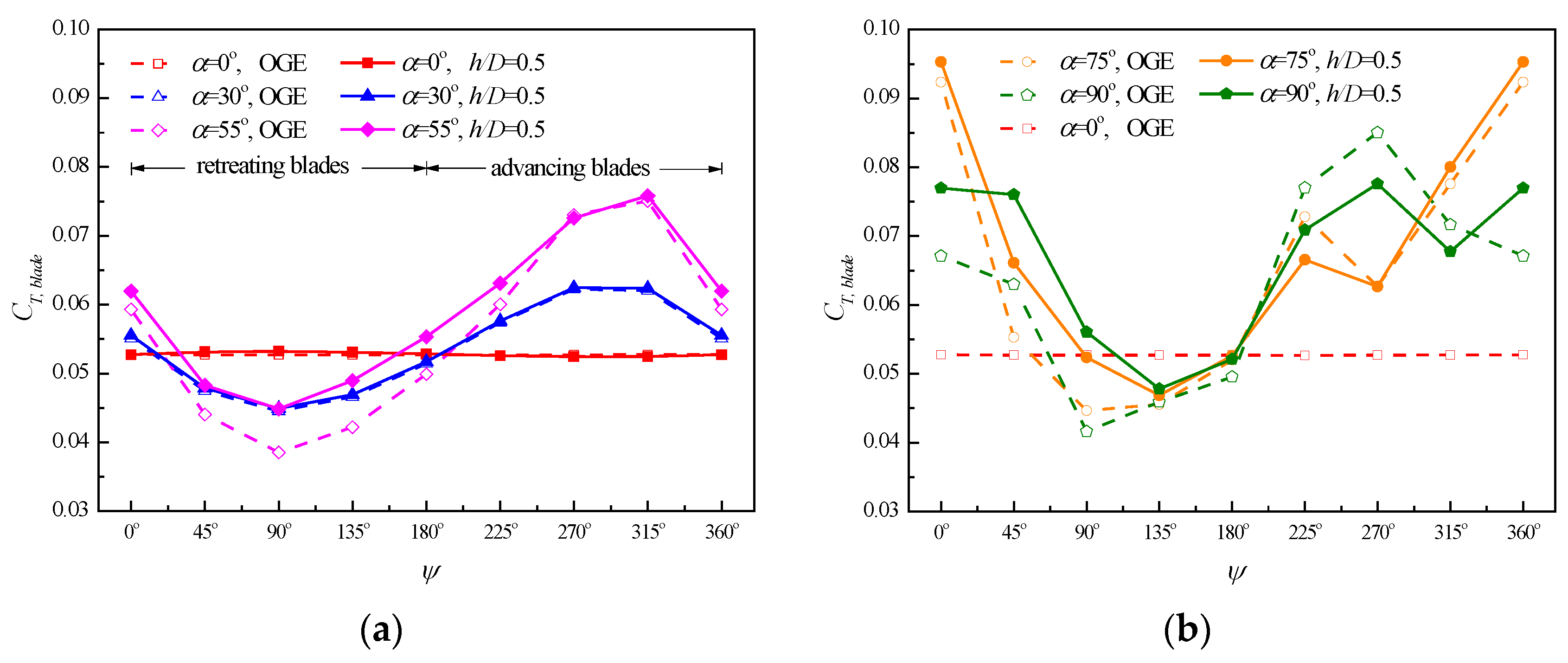
Figure 26.
Axial velocity contour and streamlines on cross sections at J = 0.5, α = 90°: (a) cross section at ξ/cd = 0.425; (b) cross section at Ψ = 6°.
Figure 26.
Axial velocity contour and streamlines on cross sections at J = 0.5, α = 90°: (a) cross section at ξ/cd = 0.425; (b) cross section at Ψ = 6°.
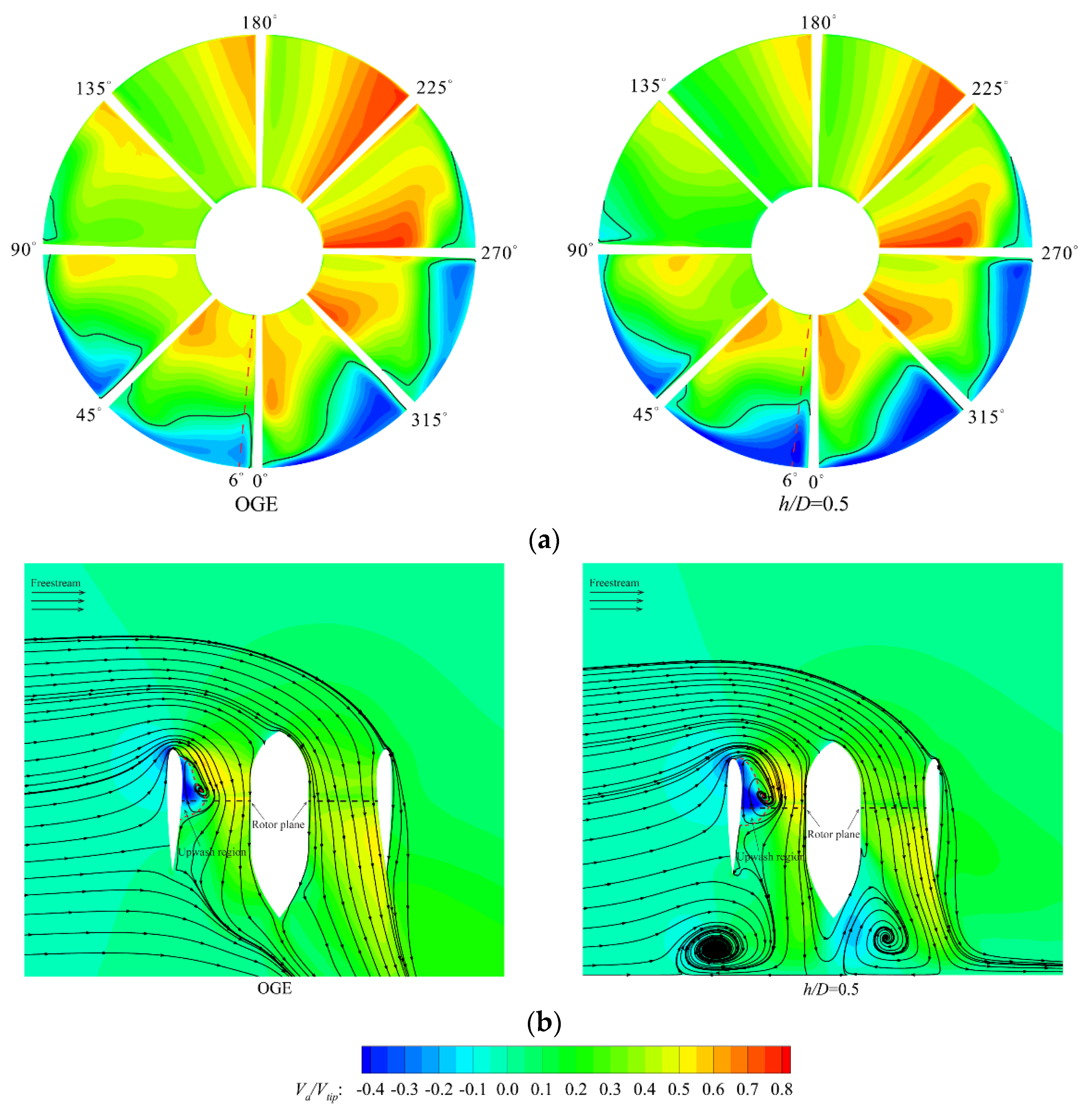
Figure 27.
Ground vortex at different advance ratios at h/D = 0.5, α = 75°: (a) J = 0.3; (b) J = 0.5. Streamlines are colored by pressure coefficients.
Figure 27.
Ground vortex at different advance ratios at h/D = 0.5, α = 75°: (a) J = 0.3; (b) J = 0.5. Streamlines are colored by pressure coefficients.

Figure 28.
Pressure coefficient contour and streamlines on symmetry plane under different conditions: (a) J = 0.3, α = 30°; (b) J = 0.1, α = 75°; (c) J = 0.3, α = 75°; (d) J = 0.5, α = 75°.
Figure 28.
Pressure coefficient contour and streamlines on symmetry plane under different conditions: (a) J = 0.3, α = 30°; (b) J = 0.1, α = 75°; (c) J = 0.3, α = 75°; (d) J = 0.5, α = 75°.
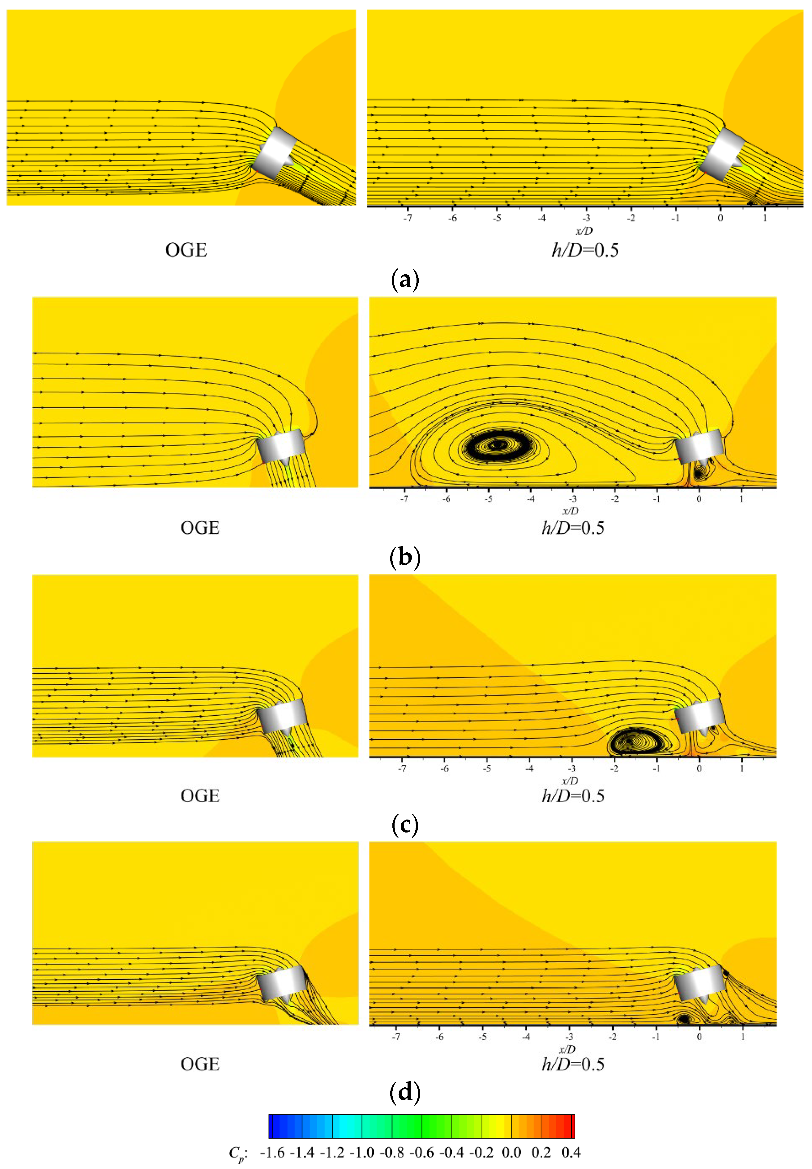
Figure 29.
Comparison of stagnation point positions on the duct between in and out of ground effect.
Figure 29.
Comparison of stagnation point positions on the duct between in and out of ground effect.


Table 1.
Main parameters of the ducted fan.
| Parameters | Value |
|---|---|
| Number of blades | 8 |
| Blade diameter Db | 0.646 m |
| Pitch angle at three-quarter radius | 39° |
| Hub diameter | 0.18 m |
| Duct chord length cd | 0.4 m |
| Duct exit diameter D | 0.704 m |
Table 2.
Comparison between CFD results of medium mesh and experimental values; Grunwald’s model in hovering.
Table 2.
Comparison between CFD results of medium mesh and experimental values; Grunwald’s model in hovering.
| Terms | CT, blades | CT, duct | CT, total | CQ |
|---|---|---|---|---|
| Experimental [9] | 0.1878 | 0.2574 | 0.4452 | 0.0295 |
| CFD | 0.1729 | 0.2442 | 0.4171 | 0.0279 |
| Discrepancy | −7.93% | −5.13% | −6.31% | −5.42% |
Table 3.
Comparison between CFD results of the medium mesh and experimental values; Grunwald’s model at J = 0.595, α = 30°.
Table 3.
Comparison between CFD results of the medium mesh and experimental values; Grunwald’s model at J = 0.595, α = 30°.
| Terms | CT, blades | CL | CX | CM | CQ |
|---|---|---|---|---|---|
| Experimental [9] | 0.1377 | 2.6195 | 0.7020 | 0.8708 | 0.0261 |
| CFD | 0.1413 | 2.3833 | 0.6516 | 0.9001 | 0.0259 |
| Discrepancy | +2.61% | −9.02% | −7.73% | +3.36% | −0.77% |
Table 4.
Comparison between results obtained via MRF method, sliding mesh method, and experiment.
| Terms | CT, blades | CT, duct | CT, total | CQ |
|---|---|---|---|---|
| Experimental [9] | 0.1878 | 0.2574 | 0.4452 | 0.0295 |
| Discrepancy of SMM | −6.34% | +2.41% | −1.28% | −2.37% |
| Discrepancy of MRF | −7.93% | −5.13% | −6.31% | −5.42% |
Table 5.
Aerodynamic performance of ducted fan when hovering out of ground effect.
| CT, blades | CT, duct | CT, total | CQ | PL (kg/kW) |
|---|---|---|---|---|
| 0.4646 | 0.6690 | 1.134 | 0.1277 | 3.828 |
Publisher’s Note: MDPI stays neutral with regard to jurisdictional claims in published maps and institutional affiliations. |
© 2022 by the authors. Licensee MDPI, Basel, Switzerland. This article is an open access article distributed under the terms and conditions of the Creative Commons Attribution (CC BY) license (https://creativecommons.org/licenses/by/4.0/).
Share and Cite
MDPI and ACS Style
Zhao, Y.; Tian, Y.; Wan, Z. Aerodynamic Characteristics of a Ducted Fan Hovering and Transition in Ground Effect. Aerospace 2022, 9, 572. https://doi.org/10.3390/aerospace9100572
AMA Style
Zhao Y, Tian Y, Wan Z. Aerodynamic Characteristics of a Ducted Fan Hovering and Transition in Ground Effect. Aerospace. 2022; 9(10):572. https://doi.org/10.3390/aerospace9100572
Chicago/Turabian StyleZhao, Yanxiong, Yun Tian, and Zhiqiang Wan. 2022. "Aerodynamic Characteristics of a Ducted Fan Hovering and Transition in Ground Effect" Aerospace 9, no. 10: 572. https://doi.org/10.3390/aerospace9100572
Note that from the first issue of 2016, this journal uses article numbers instead of page numbers. See further details here.