GAE and OBE Enhanced Interference Mitigation Techniques in LDACS

Abstract

Interference mitigation in L-band digital aeronautic communication systems from legacy users is vital due to stringent safety requirements and steady-state increase in air traffic. This paper proposes an L-band digital aeronautic communication systems receiver prototype that employs nonlinear operations to reduce the interference from the prime interference contributor distance measuring equipment. The knowledge of genie-aided estimator and optimum Bayesian estimator is utilized to propose improved and low complexity nonlinear devices, such as a genie-aided estimator enhanced pulse peak attenuator, genie-aided estimator enhanced pulse peak limiter, joint genie-aided estimator enhanced pulse peak attenuator, joint genie-aided estimator enhanced pulse peak limiter, optimum Bayesian estimator enhanced pulse peak attenuator, optimum Bayesian estimator enhanced pulse peak limiter, joint optimum Bayesian estimator enhanced pulse peak attenuator and joint optimum Bayesian estimator enhanced pulse peak limiter. The performance of the proposed methods is compared with the classical pulse blanking in terms of the received bit error rate for different signal-to-noise ratios. The proposed genie-aided estimator enhanced methods exhibited SNR saving in the range of 2 to 2.5 dB at a bit error rate of ${10}^{-1}$. At the same BER, the proposed optimum Bayesian estimator enhanced methods achieved SNR saving in the range of 2.5 to 3 dB.

1. Introduction

Aeronautical frequency spectrum loads have always been severe for aviation and are anticipated to be even more crucial with the steady increase in air traffic and the deployment of new technologies. Air-traffic expansion in Europe is expected to be over 16 million in regulation and growth and close to 20 million in global and growth. This is a 53 percent increase in regulation and growth and an 84 percent increase in global and growth in comparison with 2017 [1]. By 2040, there will be 1.5 million extra flights in demand than those which can be housed. That means about 160 million more passengers that will be unable to fly. Even with these extra or lost 1.5 million flights, the network remains highly overcrowded. Besides the annual air traffic growth and heavily saturated very high frequency band (VHF) (118 MHz to 137 MHz), the emerging technologies, such as wireless sensing and wireless avionic intra communication (WAIC) and unmanned aerial vehicle (UAV), demand a vast amount of the spectrum, as they involve the exchange of a large amount of data. However, little growth is predicted in the total size of aeronautical spectrum assignments in the long run, due to the constraints specific to the frequency allocations appropriate to support critical safety-of-life scenarios [2].

Meanwhile, disagreeing with the popular belief, studies about the spectrum occupancy revealed that large portions of the spectrum are used less frequently [3,4]. The utilization of major pieces of the spectrum is even below 10% [3]. Among them, the spectrum utilization of the aeronautic spectrum band for air–ground communications (A/G) is found to be 12.5%. The same band is anticipating severe spectrum scarcity in future. Currently, aircraft are connected to air traffic controllers and air operational controllers via voice and data communication systems. The media in voice communication are still analogue and operated via open broadcast channels without any embedded protective measures. The existing VHF double sideband amplitude modulation (DSB-AM) will be used for many more years, as it works safely and reliably with the use of low-cost communication equipment. Data communication to the cockpit is also provided by ground-based equipment operating within HF or VHF radio bands. The communication systems use narrowband radio channels with a data throughput of some kilobits per second. The existing HF and VHF data links fail to provide broadband services to flight crews now or in the future due to the lack of the available spectrum. This situation becomes a hindrance in the employment of enhanced air traffic management (ATM) operations, such as trajectory-based operations (TBO) and 4D trajectory negotiations [5]. Hence, the International Civil Aviation Organization (ICAO) recommended future communications infrastructure (FCI) to enhance the existing communication links between aircraft and ground controllers with new optimal data link protocols. This led to the development of L-band digital aeronautical communication systems (LDACS) as an inlay system between the legacy users [2] in 960–1164 MHz to face the challenge of the saturated VHF spectrum and spectrum congestion.

For further studies and enlargement, ICAO selected two candidates: LDACS1 derived from IEEE 802.16 wireless system [6] and LDACS2 derived from the global system for mobile communication (GSM) [7]. LDACS1 makes use of modern modulation techniques and advanced network protocols applied in the current commercial standards, and LDACS2 exploits the knowledge from aviation specific standards, using protocols that offer high QoS communications. Both these systems are foreseen to house the air traffic requirements without compromising the standards put forth by the aeronautical community. From the literature of L-band spectrum deployment [8,9,10,11], some of the legacy users are distance measuring equipment (DME), the military tactical air navigation (TACAN) system, and the joint tactical information distribution system (JTIDS) used for navigation aids (Figure 1). Apart from these, universal access transceiver (UAT) at 978 MHz and secondary surveillance radar (SSR), airborne collision avoidance system (ACAS) at 1030 and 1090 MHz are allotted with fixed channels. With this knowledge, the LDACS system is deployed in the L-band either as an inlay system between the legacy users, such as DME, or as an overlay system in the unoccupied spectrum [12]. Though the overlay method is less complex and selected for GSM, such as LDACS2 (960–975 MHz), spectrum scarcity is a noticeable challenge [13,14,15]. LDACS1, as an inlay approach, takes the advantage of the 1 MHz spectral gap between DME signals.

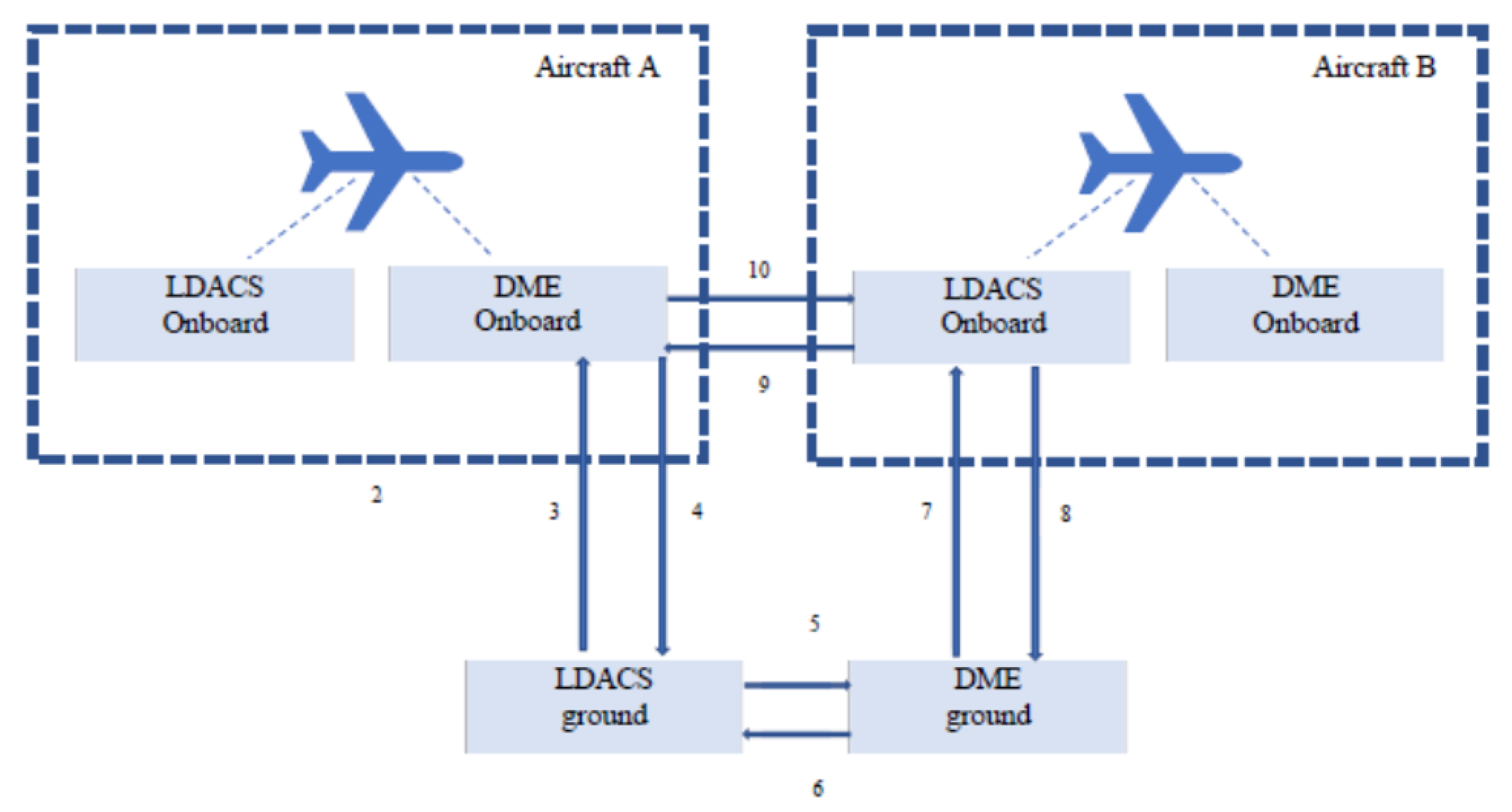
LDACS1 involves two-way communication: a forward link (FL) from the ground station (GS) to the air station (AS) and a reverse link (RL) from AS to GS. It provides frequency division duplexing (FDD) of 63 MHz spacing between FL (962–1213 MHz) and RL (1025–1150 MHz) with the opportunistic access of the paired spectrum. From Figure 2, the possible interference scenario for the LDACS1 inlay system can be recognized as follows: (a) LDACS1 FL is affected by DME GS (FL) not by DME airborne station (AS), as (RL) is not active in this part of spectrum (b) LDACS1 RL is affected by both the DME GS (FL) and DME AS (RL), (c) DME FL is affected by interference from both the LDACS1 GS (FL) and LDACS1 AS (RL), and (d) DME RL is affected with interference from LDACS1 AS (RL) not from LDACS1 GS (FL), as it is not active in this part of the spectrum [16].

Relative studies between LDACS1 and LDACS2 have shown that LDACS1 has significantly better performance than LDACS2, resulting in a conclusion that LDACS1 can be the final choice due to the capability of supporting a diversity of services and the cellular compatibility, and is referred to as LDACS [17,18]. The utilization of the L-band for aeronautical applications is very challenging, due to the occupancy of legacy systems. From the detailed study of potential levels of interference from the various legacy systems [19,20], it is found that DME is the prime legacy user occupying most of the 960 MHz to 1164 MHz spectrum. Thus, the deployment of LDACS as an inlay system with licensed users in the L-Band can cause interference to license users and vice versa. Any malfunctioning of a licensed system is a serious issue, as it is directly related to flight safety. Consequently, interference mitigation is an essential component in an LDACS receiver.

The rest of the paper is organized as follows: Section 2 briefs the literature survey about the merits and demerits of the existing DME interference mitigation techniques in LDACS. Section 3 discusses the system and noise model used for this work. Section 4 includes the mathematical functioning of proposed nonlinear estimators on the received data, and Section 5 characterizes the difference in the performance of these proposed nonlinear estimators in terms of the accuracy of the received data.

2. Related Work

Several interference mitigation techniques for LDACS are available in the literature; among these, most of the proposed schemes focus on mitigating DME interference. In 2011, Ulrich Epple et al. proposed two methods to detect and reduce DME interference. One of the methods takes advantage of the repetitive structure of the DME pulse, while the other utilizes the spectral shape of the DME signal. Simplicity is the advantage of this technique, but at the cost of losing a part of the desired signal due to pulse blanking [21]. In 2012, Hailiang Wang et al. proposed a mixed blanking technique (combination of pulse blanking and notch filter) mainly for the B2 band (1900 MHz). Though the technology has the advantage of operating in both time and frequency domain, it is more effective and safe for the B2 signal [22]. Further, Yun Bai et al. suggested a scheme that uses complementary code keying (CCK) to reduce DME interference. Though the CCK encoding has the advantage of better gain, it demands low phase distortion and a wideband channel. The acquisition time is greater, which increases the latency of the system. Moreover, the modulation used here is not a power-efficient modulation [23].

In 2014, an iterative receiver design was proposed by Q. Li et al. [24]. The design employs iterative decoding between the demodulator and decoder based on the turbo principle. Later, Martin Hirschbeck et al. proposed a block-based selective pulse blanking method, which mitigates DME interference with the employment of a designed fast filter bank [25]. Another DME mitigation method based on deformed pulse pair detection and its negation from the actual signal was proposed by Li Douzheetal et al. in 2016 [26]. Later, Khodr A. Saaifan and Werner Henkel introduced lattice signal sets to combat DME interference from aeronautical signals. The method uses precoding at the transmitter based on the lattice signal set, which modifies the shape of the DME signal spectrum; a simple clipping technique is then applied for DME mitigation [27].

The major drawback with the pulse blanking is the inter-carrier interference. A method that removes the inter-carrier interference was proposed by M. Raja et al. [12]; the method is based on the decision-directed noise estimation. Even though this method removes inter-carrier interference, the cyclic prefix reduces the throughput of transmission and leads to wastage of power. In 2019, Emad Abd-Elaty proposed LDACS-OFDM based on discrete wavelet transform (DWT) and increased sidelobe suppression [28]. The method utilizes the real nature of DME and the selective transmission of signal through the quadrature channel in the presence of DME. With the intelligence of the direct sequence spread spectrum to combine the inphase and quadrature phase, the method claims to perform DME free transmission. The computational complexity and resource requirement are the disadvantages of this method. In 2021, two methods named deep clipping and joint clipping blanking to reduce DME interference were proposed in [29]. Careful study of the existing interference mitigation techniques in LDACS exposes that there is a scope of DME mitigation in LDACS.

In 2015, a linear finite impulse response equalizer was proposed to compensate for the inter-carrier interference caused due to pulse blanking in OFDM systems [30]. Besides this, some of the existing nonlinear estimators which are still not utilized in reducing impulsive noise (or DME) in LDACS are genie-aided estimator (GAE) and optimum Bayesian estimator (OBE), to the best of our knowledge. The GAE uses statistical description of the side information as the design parameters to attain lower bounds on the bit error at the receiver [31]. GAE is expected to show better performance than any other detector working without the side information. However, an explicit detail of the side information is needed to attain this lower bound performance. The correlation of the impulsive noise or the frequency in impulsive noise arrival time are some other side information [32]. When a Gaussian source is affected with uncorrelated impulse noise, optimum system performance in terms of the signal-to-noise power ratio (SNR) can be achieved with the use of a Bayesian signal estimator. In 2013, P. Banelli proposed an optimal Bayesian estimator (OBE) explicitly for real-valued Gaussian mixture noise [33]. The method was further extended to complex signals in 2015 [34]. In our work, we analyzed the effect of GAE and OBE in DME noise reduction when the impulse noise at the received signal is estimated with a two-component Gaussian mixture model.

By utilizing the design parameters of GAE and OBE, we propose pulse peak attenuators and pulse peak limiters, which could effectively reduce DME noise when compared to conventional pulse blanking methods. Though the methods are analyzed in the LDACS background, it can also be well utilized in any other applications of OFDM multi-carrier systems, such as power-line communication (PLC), asymmetric digital subscriber lines (ADSL), 4G cellular systems (UMTS-LTE), digital video broadcasting (DVBT), and wireless local area networks (Wi-Fi) in reducing impulse noise. The new methods we put forward are as follows:

1.

GAE enhanced pulse peak attenuator (GAE PPA);

2.

GAE enhanced pulse peak limiter (GAE PPL);

3.

Joint GAE enhanced pulse peak attenuator (Joint GAE PPA);

4.

Joint GAE enhanced pulse peak limiter (Joint GAE PPL);

5.

OBE enhanced pulse peak attenuator (OBE PPA);

6.

OBE enhanced pulse peak attenuator (OBE PPA);

7.

Joint OBE enhanced pulse peak attenuator (Joint OBE PPA);

8.

Joint OBE enhanced pulse peak limiter (Joint OBE PPL).

All these methods include two basic operations.

1.

Identification of the subcarrier affected with DME noise: threshold-based detection is utilized for this operation.

2.

Processing of the signal from the affected subcarrier to remove DME interference: knowledge from genie aided estimation is utilized in methods 1, 2, 3 and 4 for the mentioned signal processing. The difference between these methods from the actual GAE is that, here, estimation is performed only for the subcarriers identified by the threshold-based detection. Similarly, the methods 5, 6, 7 and 8 well exploit the knowledge of optimum Bayesian estimation.

The advantage of all these methods compared to pulse blanking is that instead of blanking (or leaving the information), data estimation is performed to extract the information. Another advantage of these methods in comparison with the GAE/OBE estimation is the decreased complexity, as these methods work well with parameters obtained from two-component Gaussian modeling the of the received data.

3. System and Noise Model

3.1. LDACS System Model

The system model consists of the LDACS transmitter, channel which adds additive white Gaussian noise (AWGN) and DME noise, and the LDACS receiver. The detailed block diagram of the LDACS ground station transmitter is as shown in Figure 3. The random data of 91 bytes, generated from the data source, are passed through the Reed–Solomon (RS) coder, which adds 10 bytes of redundant data to the original data. The output of the RS coder further undergoes 6 bit zero padding before passing to the convolutional coder. The output of the convolutional coder is further passed through the permutation interleaver to reduce the burst errors. The blocks symbol mapper, quadrature phase shift keying (QPSK) modulation and frame composer arrange the output of the symbol mapper to the standard LDACS data frame format (S). It is to be noted that all the variables displayed in Figure 3 and Figure 4 are generated for the standard LDACS data frame format (S). The same variables with suffix ‘t’ represent the same signal for an instant ‘t’ or the $t^{th}$ OFDM symbol. For example, the output of the frame composer at an instant ‘t’ is $S_t={[S_t\left[0\right],S_t\left[1\right]\dots S_t[N-1]]}^T$ and represents the $t^{th}$ symbol of the LDACS forward link frame (S) with N orthogonal subcarriers. $S_t$ holds the random data $S_t{\left[m\right]}_{m=0,1\dots N-1}$ with zero mean and variance ${\sigma }_s^2$. The OFDM symbol $X_t={[X_t\left(0\right),X_t\left(1\right)\dots X_t(N-1)]}^T$, generated in the time domain by computing the 64-point IFFT of the data $S_t$ is also modeled with a zero mean Gaussian probability density function. Further to avoid inter-carrier interference, $N_{CP}$ number of zeros are added to the total N subcarriers, resulting in $N+N_{CP}$ subcarriers. Thus, the transmitted vector is $x{\prime }_t=[x{\prime }_t\left(0\right),x{\prime }_t\left(1\right)\prime ,x{\prime }_t(N+N_c{}_p-1)]$. The symbols X and x’ are the OFDM signals without and with cyclic prefix bits generated for the LDACS forward link frame (S).

The transmitted signal $x^{\prime }$ passes through the AWGN channel in the presence of DME interference and is received as signal $y\prime$. For each instant t, the transmitted vector $x_t^{\prime }$ is corrupted by a noise of $i_t={[i_t\left(0\right),i_t\left(1\right),\dots ,i_t(N+N_{cp-1})]}^T$, which includes the additive white Gaussian noise $W_t={[W_t\left(0\right),W_t\left(1\right),\dots ,W_t(N+N_{cp-1})]}^T$ and the impulse noise $D_t={[D_t\left(0\right),D_t\left(1\right),\dots ,D_t(N+N_{cp-1})]}^T$. Hence, the received signal for an instant ‘t’, is $y{\prime }_t={[y{\prime }_t\left(0\right),y{\prime }_t\left(1\right),y{\prime }_t(N+N_c{}_p-1)]}^T$ and can be represented as depicted in (1).

$$y{\prime }_t=x{\prime }_t+i_t$$

(1)

where

$$i_t=W_t+D_t$$

(2)

In the deployment of LDACS as an inlay system between adjacent DME channels, the major part of interference toward LDACS is DME signals. A pair of Gaussian-shaped pulses, separated by a duration of $\Delta t$, are DME signals. The duration $\Delta t$ (12 $\mathsf{\mu }$s or 36 $\mathsf{\mu }$s) and the transmission rate (30 pulse pair per second or 50 ppps) of DME signals changes with a different mode of operation of the distance measuring equipment. A pair of DME pulses in the baseband can be depicted as in (3) [35].

$$D_p\left(t\right)=e^{\frac{-\alpha t^2}{2}}-e^{\frac{-\alpha {(t-\Delta t)}^2}{2}}$$

(3)

where $\alpha =4.5\times {10}^{11}{\mathrm{s}}^{-2}$.

It has a width of 3.5 $\mathsf{\mu }$s at half of the maximum amplitude. As DME pulses are Gaussian shaped, it has same shape in the frequency domain. The spectrum is modulated with a cosine, as the pulses are always occurring pairwise. The resulting signal can be denoted as in (4) [12].

$$I_{Dp}\left(f\right)=\sqrt{\frac{8\pi }{\alpha }}{e}^{\frac{2{\pi }^2{t}^2}{\alpha }}·e^{-j\pi f\Delta t}cos(\pi f\Delta t)$$

(4)

The baseband DME pulse pairs are modulated to the relative carrier frequency of the channel to 0.5 MHz left and to the 0.5 MHz right of the LDACS system bandwidth. The total interference signal $I_{Dp}\left(t\right)$ at LDACS system for a time interval ‘t’ is from N DME stations that are operating on the 0: 5MHz offset to the center frequency of the LDACS system. Then, the DME interfering signal that affects the LDACS system can be denoted as in (5) [12].

$$I_{Dp}\left(t\right)={\mathrm{\Sigma }}_{i=0}^{N_{Dp-1}}{\mathrm{\Sigma }}_{l=0}^{N_i-1}\sqrt{P_{i,l}P(t-t_{i,l})e^{j2\pi f_{c,i}t+j{\psi }_{i,l}}}$$

(5)

where $N_{Dp}$ is the total number of interfering DME stations, $N_i$ is the total number of pulse pairs in the particular time interval for the $i^{th}$ interfering DME station, and $P_{(i,l)}$ and ${\psi }_{(i,l)}$ are the power and phase of the pulse pair respectively. $f_{(c,i)}$ is the relative carrier frequency of the $i^{th}$ interfering DME station, and $t_{(i,l)}$ is the starting time of the $l^{th}$ pulse pair of the $i^{th}$ DME station. DME noise can be reduced with the same techniques, which are used to reduce the impulse noise.

The detailed block diagram of the LDACS FL AS receiver with the proposed interference mitigation method is as shown in Figure 4. The first block in the receiver removes the cyclic prefix bits associated with the received vector $y_t\prime ={[y_t\left(0\right),y_t\left(1\right),\dots ,y_t(N+N_{C_P-1})]}^T$ resulting in vector $y_t={[y_t\left(0\right),y_t\left(1\right),\dots y_t(N-1)]}^T$. The nonlinear device present at the receiver block accomplishes suppression of DME pulses by processing the signal $y{\prime }_t$ in the time domain. In general, the resulting estimated vector can be defined as ${\widehat{x}}_t=f(y_t;{\pi }_t)$, where $f(.)$ is the nonlinear estimator for the time domain processing of input $y_t$ with ${\pi }_t$. The vector ${\pi }_t$ holds the values of parameters of $t^{th}$ OFDM block, such as the signal power ${\sigma }^2{x}_t$, noise power ${\sigma }^2{i}_t$. The nonlinear estimators discussed in this paper process the signal $y_t$ in dissimilar ways. Hence, the definition of function $f(.)$ varies with each proposed model.

The nonlinear device is operated on signal $y_t$ before the FFT processing to block the dispersion of sparse time domain impulses $D_t\left[n\right]$ over all the OFDM carriers in the frequency domain. Considering the low complexity requirement, we disregard any conceivable correlation between different time domain impulses and focus on instantaneous devices as stated by ${\widehat{x}}_t\left[n\right]=f(y_t\left[n\right];{\pi }_t$).

3.2. Impulsive Noise Models

The K-component Gaussian mixture model (K-GMM) splits any random variable to a group of K mutually exclusive Gaussian variables [36,37]. Hence, this model can be effectively applied to any ImpN distribution (Class A, $S-\alpha -S$ noises…, etc.) either estimated [38,39,40] and approximated by a K-GMM [41], or modeled with the actual equation [42,43]. The K-GMM model can be expressed mathematically with pdf,

$$f_W\left(i\right)={\mathrm{\Sigma }}_{k=0}^{K-1}{P}_k.G(i,{\sigma }_k^2)$$

(6)

where ${\left\{P_k\right\}}_{k=0,1,\dots \dots K-1}$ with ${\mathrm{\Sigma }}_{k=0}^{K-1}{p}_k=0$ are the probability of occurrence of each Gaussian component k. With the cleverness and complexity of mathematical manipulation, K-GMM with enough high K can estimate any realistic distribution as closely as needed. The component which corresponds to $k=0,i_0\approx G(i_0,{\sigma }_0^2)$ represents the thermal noise with probability of occurrence $p_0$ and thermal power ${\sigma }_0^2$. The statistical combinations of components from $k=1$ to $k=K-1$ characterize the impulse noise with the probability $p_I=1-p_0$ and noise power ${\sigma }_I^2$. When $K=2$, this model will reduce to 2-GMM with a thermal noise component $i_0\approx G(i_0,{\sigma }_0^2)$ and an impulse noise component $i_1\approx G(i_1,{\sigma }_1^2)$ (or in general $i_m\approx G(i_m,{\sigma }_m^2)$, where ${\sigma }_i>>{\sigma }_0$). The ratio of thermal noise to impulse noise can be expressed as $\Gamma =\frac{{\sigma }_0^2}{{\sigma }_I^2}$. This model is simple, widely used and assumes the presence of a strong impulsive noise as the recognition of two mutually exclusive events, with probability $p_I$ and $1-p_I$, respectively.

The received OFDM signal y can be expressed as the sum of transmitted signal $x^{\prime }$ and noise $i_k$, where $x^{\prime }$ and $i_k$ are two zero-mean independent Gaussian random variables with variances ${\sigma }_x^2$ and noise power ${\sigma }_i^2$. As discoursed in the system model, the total noise added to the Gaussian source is the sum of the additive white Gaussian noise and DME noise. This paper put forward new methods to reduce DME noise in LDACS, which utilizes the combined knowledge obtained from K-GMM and the pulse blanking method. The received signal of interest after undergoing CP removal (y) is modeled using K-GMM distribution. The parameters obtained from K-GMM modeling are effectively utilized to derive instant nonlinearity. The proposed new techniques eliminates the disadvantage of pulse blanking by using this instant nonlinearity to attenuate the noise only to the affected subcarriers in the time domain rather than blanking the whole data.

4. Nonlinear Estimators

As discussed in the system model, the nonlinear estimator has a key role in eliminating DME interference in the LDACS GS receiver. This paper deals with simple and improved designs of some nonlinear estimators $f(.)$ and comparison of its performance with the pulse blanking method. These nonlinear estimators perform instantaneous operation on the received sample (after CP removal) $y_t\left[n\right]$ by utilizing the statistical information from the signals $x_t\left[n\right](n=0,1,\dots N-1)$ and the noise component $i_t\left[n\right]$. For a sufficient number of subcarriers, the time domain OFDM symbol $x_t$ can be modeled by Gaussian pdf [44]. As the channel selected is AWGN, the useful component $y_t^{\prime }\left[n\right]$ is also Gaussian distributed.

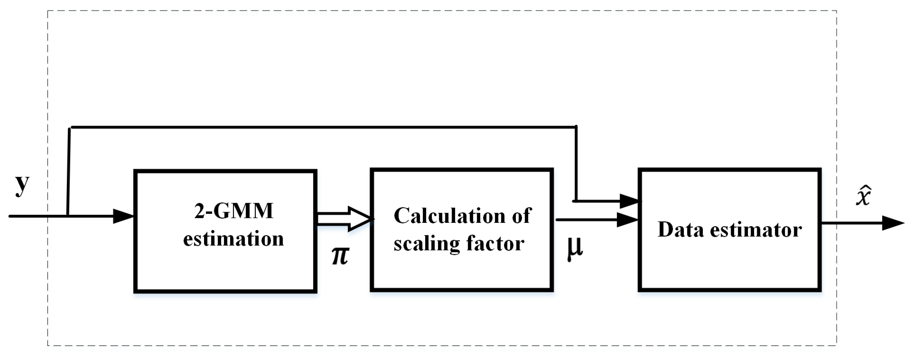
Figure 5 and Figure 6 explain how 2-GMM estimation is utilized in actual GAE/OBE and GAE/OBE enhanced pulse peak processors. In GAE/OBE, the parameters obtained after 2-GMM estimation are used to calculate the scaling factor ($\mu$). The scaling factor is ${\rho }_k$ for GAE and ${\beta }_o\left(y\right)$ for OBE. The GAE/OBE enhanced pulse peak processors perform selective nonlinear scaling with the help of a noise detector. It is possible to propose different types of nonlinear devices with various combinations of noise detectors, data estimators, and scaling factors.

In this paper, we selected single and double threshold noise detection methods. The amplitude of the received signal is compared with predefined threshold values. The different types of data estimators employed are GAE and OBE. Pulse peak attenuators use the same scaling factors used in GAE and OBE. Pulse peak limiters use different algorithm to find out different scaling factors in an iterative way. The various combinations of the above mentioned blocks result in proposing different pulse peak attenuators and limiters. The following section discusses the mathematical functioning and formulation of GAE, GAE enhanced PPA, GAE enhanced PPL, joint GAE enhanced PPA, joint GAE enhanced PPL, OBE, OBE enhanced PPA, OBE enhanced PPL, joint OBE enhanced PPA and joint OBE enhanced PPL in detail.

4.1. Genie-Aided Estimators

When the received signal is modeled with K-GMM, the genie-aided estimator (GAE) assumes the knowledge of the state of the underlying noise generation process. For any impulse noise, when modeled as properly weighted mutually exclusive Gaussian events, the GAE claims to know which is the $k^{th}$ Gaussian component of the (pdf) combination affecting at each time of epoch and causes the actual noise. The received signal y can be expressed as the sum of transmitted signal x and noise ${i|}_k$ where x and ${i|}_k$ are two zero-mean independent Gaussian random variables with variances ${\sigma }_x^2$ and ${\sigma }_i^2$. For each time epoch, the powers of the transmitted OFDM signal and receiver noise power are ${\sigma }^2{x}_t=E\left[\right|x_t\left[n\right]{|}^2]$ and ${\sigma }^2{i}_t=E\left[\right|i_t\left[n\right]{|}^2]$. Under these conditions, GAE removes the noise as per the expression in (7) [32,45].

$${\widehat{x}}_{|kG}\left(y\right)={\rho }_k.y$$

(7)

where ${\rho }_k=\frac{{\sigma }_x^2}{{\sigma }_x^2+{\sigma }_k^2}$ and,

$${\sigma }_k^2=(1+\frac{k}{A\Gamma }){\sigma }_0^2=\frac{k/A+\Gamma }{1+\Gamma }{\sigma }_i^2=\frac{k}{A\Gamma }{\sigma }_I^2+{\sigma }_0^2$$

(8)

‘A’ is the average of Gaussian mixture components. From (7), it can be understood that the linear GAE works with a variable slope at the time epoch with the knowledge (perfect and non-realistic) of the present noise state. It is to be noted that (7) is applicable for the real and imaginary parts of the complex-valued signals we are dealing with in the LDACS system. Hence, it is possible to use (9) to express the operation of GAE to complex valued data and a K-component complex Gaussian noise mixture in LDACS.

$${\widehat{x}}_{|kG}^{*}\left(y\right)={\rho }_k.\left|y\right|e^{jarg\left(y\right)}$$

(9)

The GAE is not expedient in practical systems, as the receiver is unable to predict the noise component which causes actual noise. It is possible to improve the performance of GAE by utilizing other side information, such as impulsive noise arrival time or relationship of the impulsive noise [46,47,48]. The following two estimators described in Section 4.2 and Section 4.3 exploit threshold-based noise detection along with GAE to attain a lower bound performance, especially at low SNR values, which is very important in the DME mitigation scenario.

4.2. GAE Enhanced Pulse Peak Attenuator

The proposed instantaneous nonlinear device GAEPPA identifies the knowledge of the state of the underlying noise generation process, the same as in GAE. The proposed GAE enhanced PPA uses this knowledge to attenuate the input y only when the amplitude of the received signal exceeds the threshold value. In other words, it utilizes the knowledge obtained from GAE and threshold-based noise detection method. Hence, the operation of GAE enhanced PPA can be expressed as follows:

$${\widehat{x}}_{\left|kGA\right|}\left(y\right)=\left\{\begin{array}{cc}y\hfill & \mathrm{if}\left|y\right|\le {\alpha }_{th}\hfill \\ {\rho }_k.y\hfill & \mathrm{otherwise}.\hfill \end{array}\right.$$

(10)

Thus, GAE enhanced PPA improves the performance of the pulse blanking method, as it attenuates the signal values, which exceeds the threshold value rather than blanking the received signal, not causing the useful data loss present at carriers. Additionally, this method is less complex, as it works well even with 2-GMM modeling of the DME pulse. The device is well suited to process complex data signals as in LDACS with the modified equation as follows:

$${\widehat{x}}_{\left|kGA\right|}^{*}\left(y\right)=\left\{\begin{array}{cc}\left|y\right|e^{jarg\left(y\right)}\hfill & \mathrm{if}\left|y\right|\le {\alpha }_{th}\hfill \\ {\rho }_k.\left|y\right|e^{jarg\left(y\right)}\hfill & \mathrm{otherwise}.\hfill \end{array}\right.$$

(11)

4.3. GAE Enhanced Pulse Peak Limiter

GAE enhanced PPL is a modified or improved form of GAE enhanced PPA, where a selective attenuation of the received signal is performed continuously until there exist no amplitude values greater than threshold value ${\alpha }_{th}$. The repeated attenuation will not affect the subcarriers which are not affected with the impulse noise, as the attenuation is applied only to the subcarriers whose amplitude is greater than ${\alpha }_{th}$. The selective attenuation process is possible in two ways. To detail both the ways, we formulated two different algorithms, included in Appendix B.1 and Appendix B.2. The execution of these two algorithms resulted in two types of pulse peak limiters, named Type 1 GAEPPL and Type 2 GAEPPL.

Execution of Algorithm A1 in Appendix B.1 resulted in Type 1 GAE Enhanced PPL, which process the input signal y and delivers output ${\widehat{x}}_k\left(y\right)$ as stated in (12).

$${\widehat{x}}_{\left|kGL\right|}\left(y\right)=\left\{\begin{array}{cc}y\hfill & \mathrm{if}\left|y\right|\le {\alpha }_{th}\hfill \\ {\rho }_{mod}.y\hfill & \mathrm{otherwise}.\hfill \end{array}\right.$$

(12)

where ${\rho }_{mod}=\frac{{\sigma }_x^2}{{\sigma }_x^2+N.{\sigma }_k^2}$.

Here, the value of N varies directly with the difference in power of the received signal and threshold peak detection value at each instant. From Algorithm A1, it is clear that the maximum value of N is obtained when the maximum output amplitude is limited to ${\alpha }_{th}$. With this knowledge, the value of $N_{max}$ is derived as in (13). The steps are included in Appendix A.1,

$$\begin{array}{c}\hfill N_{max}=\frac{{\sigma }_x^2{\left(\right|y|}_{max}-{\alpha }_{th})}{{\alpha }_{th}{\sigma }_k^2}\end{array}$$

(13)

Similarly, the second method to perform pulse peak limiting is detailed in Algorithm A2 (Appendix B.2). The execution of this algorithm resulted in Type 2 GAEPPL. The mathematical functioning of Type 2 GAEPPL is as in (14)

$$\begin{array}{c}\hfill \begin{array}{c}\hfill {\widehat{x}}_{\left|kGLs\right|}\left(y\right)=\left\{\begin{array}{cc}y\hfill & \mathrm{if}\left|y\right|\le {\alpha }_{th}\hfill \\ M.{\rho }_k.y\hfill & \mathrm{otherwise}.\hfill \end{array}\right.\end{array}\end{array}$$

(14)

From the steps discussed in Algorithm A2, the maximum value of M is simply derived as in (15). The derivation part is mentioned in Appendix A.2.

$$\begin{array}{c}\hfill M_{max}=\frac{{\alpha }_{th}}{{\rho }_k.{\left|y\right|}_{max}}\end{array}$$

(15)

Similar to GAE enhanced PPA, GAE enhanced pulse peak limiters also reduce the drawback of the pulse blanking method with less complexity. Both of these methods are applicable to perform scaling of complex valued data with a slight change in Equation (12) and Equation (14), resulting in (16) and (17), respectively.

$${\widehat{x}}_{\left|kGL\right|}^{*}\left(y\right)=\left\{\begin{array}{cc}\left|y\right|e^{jarg\left(y\right)}\hfill & \mathrm{if}\left|y\right|\le {\alpha }_{th}\hfill \\ {\rho }_{mod}.\left|y\right|e^{jarg\left(y\right)}\hfill & \mathrm{otherwise}.\hfill \end{array}\right.$$

(16)

where ${\rho }_{mod}=\frac{{\sigma }_x^2}{{\sigma }_x^2+N.{\sigma }_k^2}$.

$${\widehat{x}}_{\left|kGLs\right|}^{*}\left(y\right)=\left\{\begin{array}{cc}\left|y\right|e^{jarg\left(y\right)}\hfill & \mathrm{if}\left|y\right|\le {\alpha }_{th}\hfill \\ M.{\rho }_k.\left|y\right|e^{jarg\left(y\right)}\hfill & \mathrm{otherwise}.\hfill \end{array}\right.$$

(17)

In (16) and (17), the definition for ${\rho }_{mod}$ and M remains same as that used in (12) and (14).

4.4. Joint GAE Enhanced Pulse Peak Attenuator and Limiter

The joint GAE enhanced pulse peak attenuator/limiter performs the operation of GAE enhanced attenuator/limiter only when the absolute amplitude of the received signal occurs in between two threshold values. The lower threshold value $\left({\alpha }_{thl}\right)$ is the same threshold value $\left({\alpha }_{th}\right)$ used for the GAE enhanced pulse peak attenuator/limiter. As the high amplitude of DME noise causes high amplitude of the received signal, the signal contained in subcarriers whose amplitude exceeds the upper threshold $\left({\alpha }_{thu}\right)$ value is made to zero or blanked. The operation of the joint GAE enhanced pulse peak attenuator is mathematically depicted as in (18).

$${\widehat{x}}_{\left|kJGA\right|}^{*}\left(y\right)=\left\{\begin{array}{cc}\left|y\right|e^{jarg\left(y\right)}\hfill & \mathrm{if}\left|y\right|\le {\alpha }_{thl}\hfill \\ {\rho }_k\left|y\right|e^{jarg\left(y\right)}\hfill & \mathrm{if}{\alpha }_{thl}<\left|y\right|\le {\alpha }_{thu}\hfill \\ 0\hfill & \mathrm{for}\left|y\right|>{\alpha }_{thu}\hfill \end{array}\right.$$

(18)

Joint GAEPPL can be seen as a cascaded combination of a pulse blanker with a threshold cut-off frequency of ${\alpha }_{thu}$ followed by GAEPPL with a threshold cut-off frequency of ${\alpha }_{thl}$. Hence, with the use of Algorithms A1 and A2, it is possible to design Type 1 and Type 2 Joint GAE PPL. The functioning of Type 1 and 2 Joint GAE enhanced pulse peak limiter is expressed as in (19) or in (20),

$${\widehat{x}}_{\left|kJGL\right|}^{*}\left(y\right)=\left\{\begin{array}{cc}\left|y\right|e^{jarg\left(y\right)}\hfill & \mathrm{if}\left|y\right|\le {\alpha }_{thl}\hfill \\ {\rho }_{mod}\left|y\right|e^{jarg\left(y\right)}\hfill & \mathrm{if}{\alpha }_{thl}<\left|y\right|\le {\alpha }_{thu}\hfill \\ 0\hfill & \mathrm{for}\left|y\right|>{\alpha }_{thu}\hfill \end{array}\right.$$

(19)

$${\widehat{x}}_{\left|kJGLs\right|}^{*}\left(y\right)=\left\{\begin{array}{cc}\left|y\right|e^{jarg\left(y\right)}\hfill & \mathrm{if}\left|y\right|\le {\alpha }_{thl}\hfill \\ M.{\rho }_k\left|y\right|e^{jarg\left(y\right)}\hfill & \mathrm{if}{\alpha }_{thl}<\left|y\right|\le {\alpha }_{thu}\hfill \\ 0\hfill & \mathrm{for}\left|y\right|>{\alpha }_{thu}\hfill \end{array}\right.$$

(20)

where ${\rho }_{mod}$ and M are same as defined section GAE PPL.

4.5. OBE

Bayesian estimators are useful in any Gaussian source affected by any Gaussian-mixture noise [33]. The time domain OFDM signal x can be approximated by Gaussian pdf, $f_X\left(x\right)=G(x;{\sigma }_x^2)=\frac{x^2/2{\sigma }_X^2}{\sqrt{2\pi }\sigma X}$. The complex valued received signal $y_t\left[n\right]$ at the receiver side has real and imaginary part $y_{t,R}\left[n\right]$ and $y_{t,I}\left[n\right]$, respectively. Consider that y represents distinctly either the real or the imaginary part of $y_t\left[n\right]$. When the received signal of interest is modeled or approximated as a Gaussian pdf or K-component pdf, the minimum mean square error Bayesian estimators can be effectively utilized along with the knowledge of the signal $x_t$. By exploiting the statistical dependency between X and i, it is possible to write $f_{\left(Y\right|X)}\left(y\right)=f_i(y-x)$ and $G(y;{\sigma }_{yk}^2)=G(y;{\sigma }_x^2)*G(y;{\sigma }_k^2)$. Here, * stands for convolution operation. Thus the received noise power ${\sigma }_{yk}^2$ is the sum of the signal power ${\sigma }_x^2$ and $k^{th}$ Gaussian component noise power ${\sigma }_k^2$

$$\begin{array}{c}\hfill {\sigma }_{yk}^2={\sigma }_x^2+{\sigma }_k^2\end{array}$$

(21)

Considering all this information, the Bayesian estimated value can be expressed as in (22), which also expresses the dependency of OBE with signal power ${\sigma }_x^2$ and each noise component ${\sigma }_k^2$ along with probability of occurrence of each component ($p_k$).

$$\begin{array}{c}\hfill \begin{array}{cc}\hfill {\widehat{x}}_{k}o\left(y\right)& =E_{X|Y}\left\{x\right\}=\frac{E_{X,Y\left|X\right\{x\}}}{f_Y\left(y\right)}=\frac{\mathrm{\Sigma }{P}_k{E}_x{Y}_k|X\left\{x\right\}}{f_Y\left(y\right)}\hfill \\ & =\frac{{\mathrm{\Sigma }}_{k=0}^{K-1}{\rho }_k{p}_{k}G(y;{\sigma }_{yk}^2)}{{\mathrm{\Sigma }}_{k=0}^{K-1}{p}_{k}G(y;{\sigma }_{yk}^2)}\hfill \\ \hfill & ={\beta }_o\left(y\right).y\hfill \end{array}\end{array}$$

(22)

where

$$\begin{array}{c}\hfill \begin{array}{c}\hfill {\beta }_o\left(y\right)=\frac{{\mathrm{\Sigma }}_{k=0}^{K-1}{\rho }_k{p}_{k}G(y;{\sigma }_{yk}^2)}{{\mathrm{\Sigma }}_{k=0}^{K-1}{p}_{k}G(y;{\sigma }_{yk}^2)}\end{array}\end{array}$$

(23)

and $f_Y\left(y\right)=f_X\left(y\right)*f_i\left(y\right)$. From (22), it is clear that the attenuation factor of the Bayesian estimator can be viewed as the weighted sum of K number of GAE linear attenuators, where the nonlinear weights are $\frac{p_{k}G(y;{\sigma }_{yk}^2)}{{\mathrm{\Sigma }}_{k=0}^{K-1}{p}_{k}G(y;{\sigma }_{yk}^2)}$. The output expression of the Bayesian estimator (22) can be easily generalized as shown in (24) for complex valued signal operations.

$$\begin{array}{c}\hfill {\widehat{x}}_k^{*}o\left(y\right)=\frac{{\mathrm{\Sigma }}_{k=0}^{K-1}{\rho }_k{p}_{k}G\left(\right|y|;{\sigma }_{yk}^2)}{{\mathrm{\Sigma }}_{k=0}^{K-1}{p}_{k}G\left(\right|y|;{\sigma }_{yk}^2)}\left|y\right|e^{jarg\left(y\right)}\end{array}$$

(24)

where y is the complex valued signal expressed by $y=y_r+j{y}_i$ and $\left|y\right|$ is the signal envelope.

4.6. OBE Enhanced Pulse Peak Attenuator

The proposed OBE aided PPA works exactly like OBE, which uses the noise information from 2-GMM distribution when the envelope of nonlinear input is greater than the peak threshold detection value (${\alpha }_{th}$). This device does not operate on the complex data at the input and passes to the output as it is when the above-mentioned condition is not accomplished. This new estimator improves the pulse blanking method by attenuating the complex data rather than discarding the information present at that subcarrier. In another way, it reduces the complex computations in the employment of OBE by utilizing the knowledge of parameters obtained from 2-GMM modeling along with the details from pulse blanking. The operation of the proposed estimator can be expressed mathematically as follows:

$${\widehat{x}}_{\left|kOA\right|}\left(y\right)=\left\{\begin{array}{cc}y\hfill & \mathrm{if}\left|y\right|\le {\alpha }_{th}\hfill \\ {\beta }_o\left(y\right).y\hfill & \mathrm{otherwise}.\hfill \end{array}\right.$$

(25)

It is possible to use this proposed OBE enhanced PPA for processing complex valued signal as well. The mathematical statement for this operation is as given in (26) without altering the definition of ${\beta }_O$.

$${\widehat{x}}_{kOA}^{*}\left(y\right)=\left\{\begin{array}{cc}\left|y\right|\hfill & \mathrm{if}\left|y\right|e^{jarg\left(y\right)}\le {\alpha }_{th}\hfill \\ {\beta }_o\left(y\right).\left|y\right|.e^{jarg\left(y\right)}\hfill & \mathrm{otherwise}.\hfill \end{array}\right.$$

(26)

4.7. OBE Enhanced Pulse Peak Limiter

OBE enhanced PPL is an altered or upgraded form of OBE enhanced PPA. The pulse peak limiting is performed by the repeated selective attenuation of the received signal until the resulting signal holds no amplitude values greater than the threshold value ${\alpha }_{th}$. As the repeated attenuation is performed only for the subcarriers which exceed the threshold amplitude value, it will not disturb the subcarriers where the information is not affected by DME interference. The OBE enhanced PPL process the input signal y and delivers output $x{}_k(y$) as stated in (27).

$${\widehat{x}}_{\left|kOL\right|}\left(y\right)=\left\{\begin{array}{cc}y\hfill & \mathrm{if}\left|y\right|\le {\alpha }_{th}\hfill \\ {\beta }_{mod}\left(y\right).y\hfill & \mathrm{otherwise}.\hfill \end{array}\right.$$

(27)

where

$$\begin{array}{c}\hfill \begin{array}{c}\hfill {\beta }_{mod}\left(y\right)=\frac{{\alpha }_{th}}{\left(\right|y\left|\right)}\end{array}\end{array}$$

(28)

Here, the value of ${\beta }_{mod}\left(y\right)$ can be varied in two ways so that ${\beta }_{mod}\left(y\right)$. $\left|y\right|$ becomes equal to ${\alpha }_{th}$. The two methods are detailed in Algorithms A3 and A4 included in Appendix B.3 and Appendix B.4. Using the steps in Algorithms A3 and A4 results in two types of OBE enhanced pulse peak limiters.

From Algorithm A3, it is clear that the value of noise power components ${\sigma }_k^2$ is boosted Q times so that the term the output at the nonlinear becomes equal to the threshold peak detection value. In this case, the modified scaling factor ${\beta }_{mod}\left(y\right)$ can be expressed as in (29).

$$\begin{array}{c}\hfill {\beta }_{mod}\left(y\right)=\frac{{\mathrm{\Sigma }}_{k=0}^{K-1}{\rho }_{mod}{p}_{k}G(y;{\sigma }_{ykmod}^2)}{{\mathrm{\Sigma }}_{k=0}^{K-1}{p}_{k}G(y;{\sigma }_{ykmod}^2)}\end{array}$$

(29)

where ${\rho }_{mod}=\frac{{\sigma }_x^2}{{\sigma }_x^2+Q.{\sigma }_k^2}$ and ${\sigma }_{ykmod}^2={\sigma }_x^2+Q.{\sigma }_k^2.$

Algorithm A4 details the second method to perform pulse peak limiting of the selected samples. With the use of this algorithm, realization of Type 2 OBEPPL has occurred. From Algorithm A4, it is understood that P multiples of ${\beta }_O$ are considered ${\beta }_{mod}$ for limiting the pulse peak. The maximum value of P for limiting the output is derived as in (31). The steps to obtain (31) are included in Appendix A.3.

Both of these methods are adaptable for performing operations on complex valued OFDM data signals as in LDACS. This can be stated mathematically as in (30),

$${\widehat{x}}_{\left|kOL\right|}^{*}\left(y\right)=\left\{\begin{array}{cc}\left|y\right|e^{jarg\left(y\right)}\hfill & \mathrm{if}\left|y\right|\le {\alpha }_{th}\hfill \\ {\beta }_{mod}\left(y\right).\left|y\right|e^{jarg\left(y\right)}\hfill & \mathrm{otherwise}.\hfill \end{array}\right.$$

(30)

$$\begin{array}{c}\hfill P_{max}=\frac{{\alpha }_{th}}{{\beta }_o\left(y\right)\left|y_{max}\right|}\end{array}$$

(31)

It is to be noted that the function ${\beta }_{mod}$ remains unaltered when the proposed nonlinear device process complex OFDM data. The variables P and Q can accept values 1, 2, 3, etc.

4.8. Joint OBE Enhanced Pulse Peak Attenuator and Limiter

Joint OBE enhanced pulse peak attenuator and limiter is similar to the OBE enhanced attenuator and limiter when the absolute amplitude of the received signal rests in between the lower threshold value $\left({\alpha }_{thl}\right)$ and threshold value $\left({\alpha }_{thu}\right)$. Hence the non linear functioning of the joint OBE enhanced pulse peak attenuator is mathematically depicted as in (32),

$${\widehat{x}}_{\left|kJOA\right|}^{*}\left(y\right)=\left\{\begin{array}{cc}\left|y\right|e^{jarg\left(y\right)}\hfill & \mathrm{if}\left|y\right|\le {\alpha }_{thl}\hfill \\ {\beta }_o\left(y\right)\left|y\right|e^{jarg\left(y\right)}\hfill & \mathrm{if}{\alpha }_{thl}<\left|y\right|\le {\alpha }_{thu}\hfill \\ 0\hfill & \mathrm{for}\left|y\right|>{\alpha }_{thu}\hfill \end{array}\right.$$

(32)

Similarly the functioning of the joint OBE enhanced pulse peak limiter is expressed as in (33),

$${\widehat{x}}_{\left|kJOL\right|}^{*}\left(y\right)=\left\{\begin{array}{cc}\left|y\right|e^{jarg\left(y\right)}\hfill & \mathrm{if}\left|y\right|\le {\alpha }_{thl}\hfill \\ {\beta }_{mod}\left(y\right)\left|y\right|e^{jarg\left(y\right)}\hfill & \mathrm{if}{\alpha }_{thl}<\left|y\right|\le {\alpha }_{thu}\hfill \\ 0\hfill & \mathrm{for}\left|y\right|>{\alpha }_{thu}\hfill \end{array}\right.$$

(33)

where ${\beta }_{mod}\left(y\right)$ is the same as the defined section OBE PPL. Hence, it is possible to realize this estimator in two ways with different definitions of ${\beta }_{mod}\left(y\right)$.

5. Results and Discussions

This section discusses the variation in performance of proposed nonlinear estimators GAEPPA, GAEPPL, JGAEPPA, JGAEPPL, OBEPPA, OBEPPL, JOBEPPA and JOBEPPL in reducing DME interference when employed in OFDM-based LDACS communication. The discussion is based on the results obtained from the Matlab simulation of the LDACS forward link communication prototype. The performance of proposed methods is compared with the existing pulse blanking method in terms of variation in BER at the LDACS receiver for different SNRs. The mathematical model of LDACS FL GS transmitter (Figure 3) and LDACS FL AS receiver (Figure 4) are developed in accordance with standards of the LDACS system for all the inner building blocks.

At the transmitter side, random data of 91 bytes are generated by the data source and given as the input of RS coder (91,101) for external coding. Once external encoding is performed by the RS encoder, 6-bit zero padding is performed before passing through internal encoding by the convolutional encoder (171,133). The encoded bits from the output of the convolutional coder with a native coding rate of half are further interleaved (using the permutation interleaver), mapped to symbols (using symbol mapper). The mapped symbols form complex values when it passes through the QPSK modulation block. The frame composer block forms the LDACS FL Data/CC frame with proper insertion of pilot values (158), null values (728) and complex data values (2442) over a total of 3328 subcarriers. Further, the time domain composite waveform of this OFDM frame is generated by passing the frame through the IFFT block of length 64. The effect of the introduction of IFFT (windowing) is canceled by adding 16 cyclic prefix bits.

Table 1. OFDM Parameters for LDACS1 [12].

OFDM Parameters	Values
Effective RF BW (FL or RL)	498.05 KHz
FFT Size $N_{FFT}$	64
Sampling time $T_{sa}$	1.6 $\mathsf{\mu }$s
Subcarrier spacing f	9.765625 KHz
Used subcarriers $N_u$	50
Useful symbol time $N_u$	102.4 $\mathsf{\mu }$s
Cyclic prefix time $T_{cp}$	17.6 $\mathsf{\mu }$s
Total OFDM symbol time $T_s$	120 $\mathsf{\mu }$s
Guard time $T_g$	4.8 $\mathsf{\mu }$s
Windowing time $T_w$	12.2 $\mathsf{\mu }$s
Number of lower frequency guard subcarriers $N_{g,left}$	7
Number of higher frequency guard subcarriers
Lower frequency guard subcarriers $N_{g,right}$	6
Total FFT BW $B_g$	625 KHz

holds the OFDM system parameters used in this simulation study.

The block diagram of the proposed LDACS receiver is shown in Figure 4. Each block of the receiver is designed in such a way that, it is capable of retrieving the data transmitted from the transmitter if there is no noise in the channel. From the received data, the cyclic prefix bits are removed initially. The resulting data are further converted into the frequency domain so that pilot removal and complex data segregation from corresponding subcarriers can be done at the frame decomposer block. The complex data values further undergo QPSK demodulation and symbol de-mapping to obtain the bitstreams. The bitstreams are de-interleaved and decoded using the de-interleaver and vitterbi decoder, respectively. From the output of the vitterbi decoder, redundant bits are removed and decoded, using the RS decoder to get the original data.

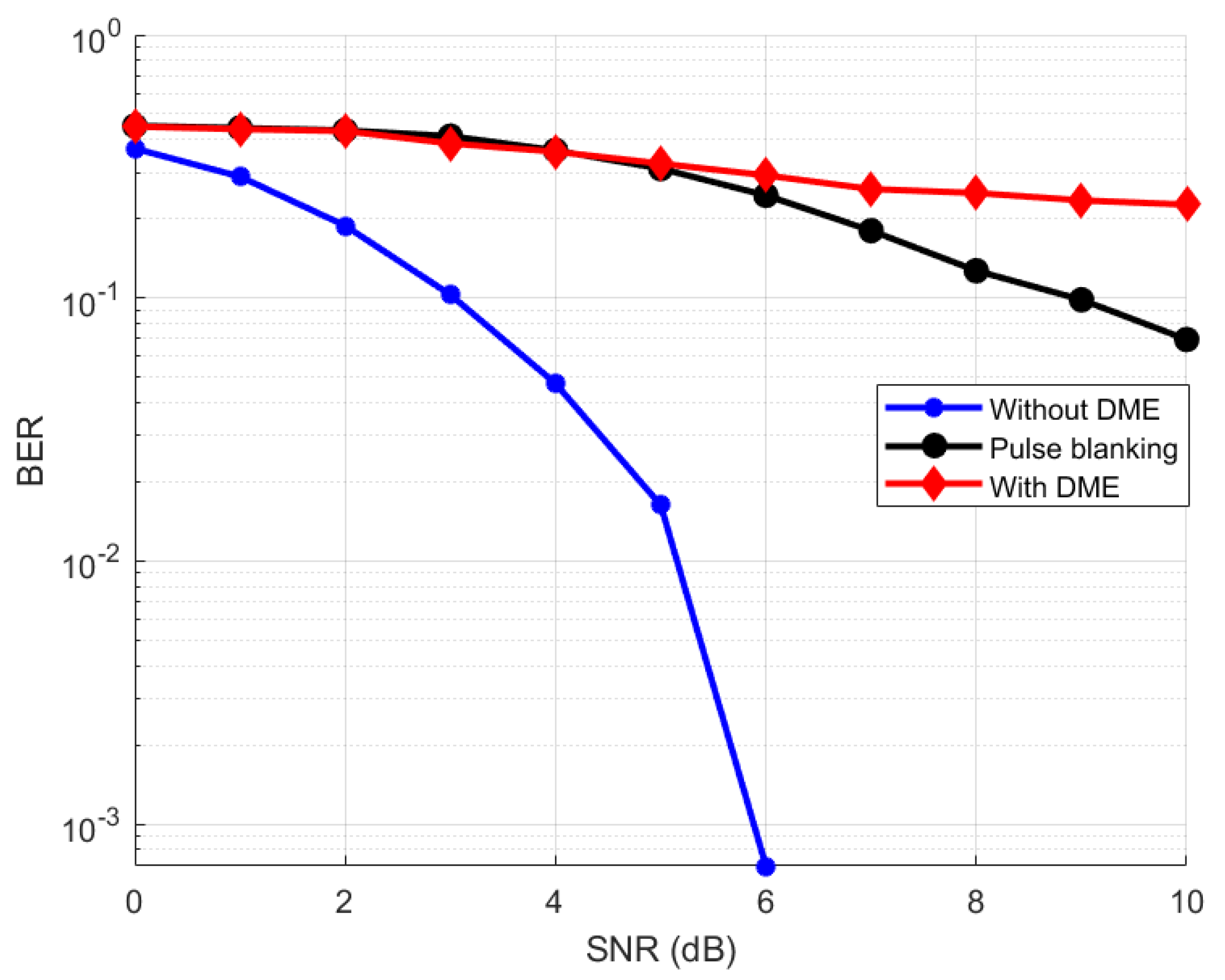
In order to analyze the performance degradation of the LDACS FL AS receiver due to DME interference, the AWGN channel is considered. The BER variation of the received signal when passed through the AWGN channel without the influence of the DME interference is obtained as shown in Figure 7. For the study of interference on LDACS, DME signals are generated in accordance with (3) for a duration $\Delta t$ of 12 $\mathsf{\mu }$s. The baseband DME pulse pairs are modulated to the relative carrier frequency of the channel to 0.5 MHz left and to the 0.5 MHz right of the LDACS1 system bandwidth. A reduction in performance of the LDACS FL AS receiver can be observed when DME noise is allowed to affect the transmitted data. Figure 7 also shows how the existing simple noise reduction method (pulse blanking) improved the performance of the receiver. The threshold value used for the pulse blanking method is 0.3 [12]. Careful analysis of Figure 7 reveals the fact that the pulse blanking technique showed a significant improvement in the performance of the receiver at the high SNR powers and a slight decrease at low SNR values.

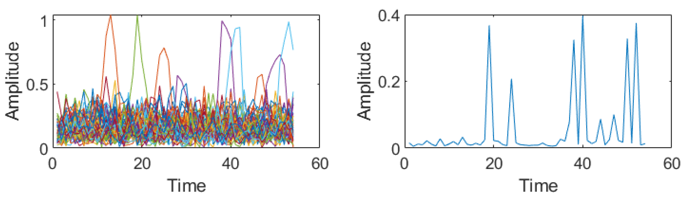
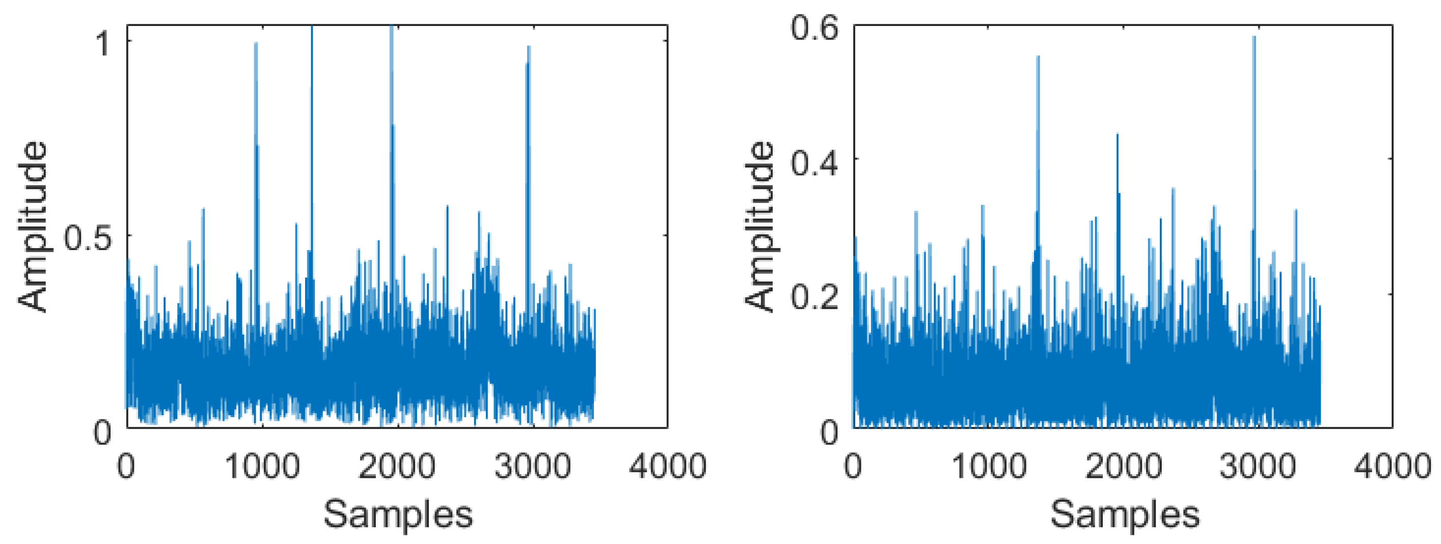
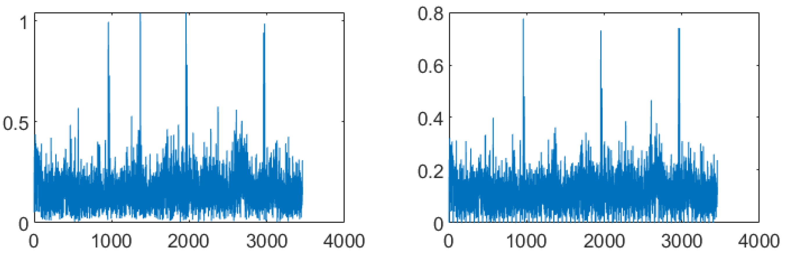
K-GMM modeling of the received signal is inevitable for the proper functioning of any of the proposed GAE enhanced pulse processing techniques. In our proposed methods, we considered the simplest K-GMM method, which splits the total noise associated with each OFDM symbol into a statistical combination of two components. Thus, with the help of 2-GMM modeling of the received OFDM data (after CP removal), the total noise power in the channel for each OFDM symbol is separated into two mutually exclusive Gaussian variables. From (6), it can be easily recognized that with 2-GMM, the resulting components are thermal noise corresponding to $k=0,i_0\approx G(i_0,{\sigma }_0^2)$ and impulse noise (DME noise) $k=1,i_1\approx G(i_1,{\sigma }_1^2)$. The resulting variances ${\sigma }_0^2$ and ${\sigma }_1^2$, along with their probability of occurrences $p_0$ and $p_1$ are used to calculate ${\sigma }_k^2$ using (8) and is displayed in Figure 8 (right). Comparing these values of ${\sigma }_k^2$ with Figure 8 (left), which shows the absolute values of CP removed OFDM symbols of the LDACS FL Data/CC frame, it is clearly understood that ${\sigma }_k^2$ could predict the OFDM symbols affected with impulse noise, though not perfectly.

The value of ${\sigma }_k^2$ obtained from the 2-GMM modeling of the signal y and the variance of transmitted signal ${\sigma }_x^2$ for each OFDM symbol is utilized in calculating the nonlinear scaling factor ${\rho }_k$ in (9). From Figure 9, it can be observed that though GAE could reduce the amplitude of the impulsive noise, it is not sufficient to remove the DME noise. Hence, no reduction in BER is observed from the DME noise affected system.

Though the GAE block works, it fails to eliminate DME noise appropriately when the complex received signal is modeled using the 2-GMM distribution. One of the possible reasons behind this could be the minimum value of K = 2, which is used to model the received complex data, which leads to inaccurate scaling of subcarriers. Another reason could be the scaling of data in subcarriers that are not affected by impulse noise, as each value of ${\sigma }_k^2$ is the same for all the subcarriers in a single OFDM symbol. Hence, though the GAE claims to predict the active component at each time epoch, it is not always practical. It may be possible to overcome these two reasons either by increasing the K value in K-GMM or by applying nonlinear scaling only to the noise-affected subcarriers. The second possibility gives way to the development of GAE enhanced PPA discussed in the following section.

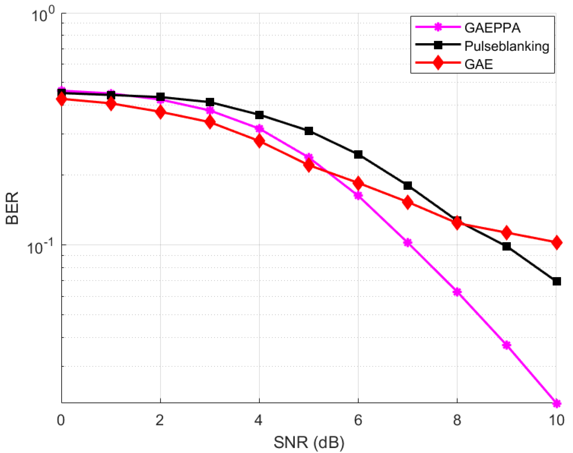
The performance of the GAE can be improved with the knowledge of other side information [32]. To avoid the unwanted scaling happening with data present over subcarriers that are not actually affected with noise, we applied the nonlinear scaling of GAE (11) only to subcarriers that are affected with impulse noise. The schematic of the absolute value of complex data input to GAE enhanced PPA and the obtained output is shown in Figure 10 (left) and Figure 10 (right) respectively. We utilized the basic logic applied in the pulse blanking technique to identify the subcarriers affected by DME noise. Thus when the nonlinear scaling is applied only to selected subcarriers as in (11), a reduction in BER is achieved in comparison to pulse blanking. The results are shown in Figure 11. Thus, GAE enhanced PPA could achieve a better result in terms of reduction in BER with variation in SNR, compared to both GAE and pulse blanking.

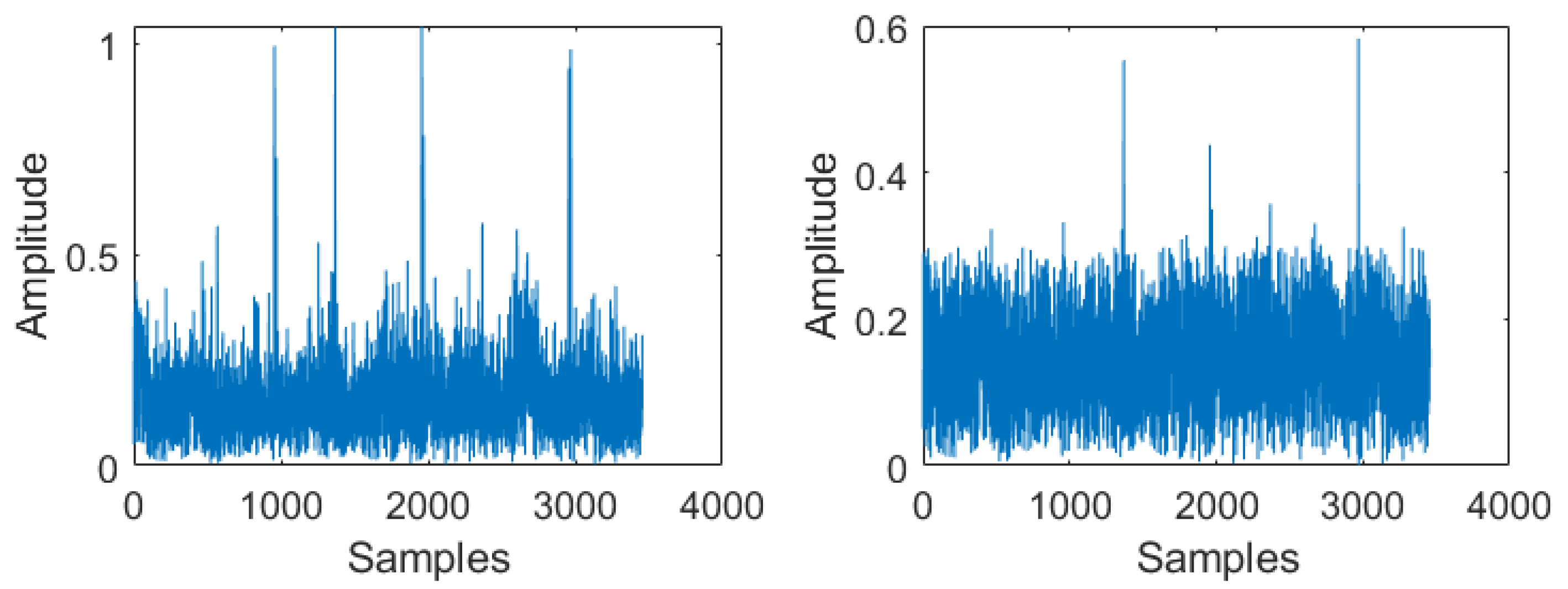
GAE enhanced PPL performed nonlinear scaling only to the subcarriers, which are affected with impulse noise in such a way that the amplitude of the resulting signal after nonlinear scaling is at least equal to the threshold value used for detecting the pulse peak (12). Comparing Figure 10 (right) and Figure 12 (right), we could clearly observe that the nonlinear output displays in Figure 12 (right) is similar to Figure 10 (right) with the maximum output value limited to the threshold value used for identifying the affected subcarriers. As discussed in the system model number, this limiting operation is possible in two ways as in (12) or (14). Performance comparison of these proposed methods with GAEPPA and conventional pulse blanking are shown in Figure 13.

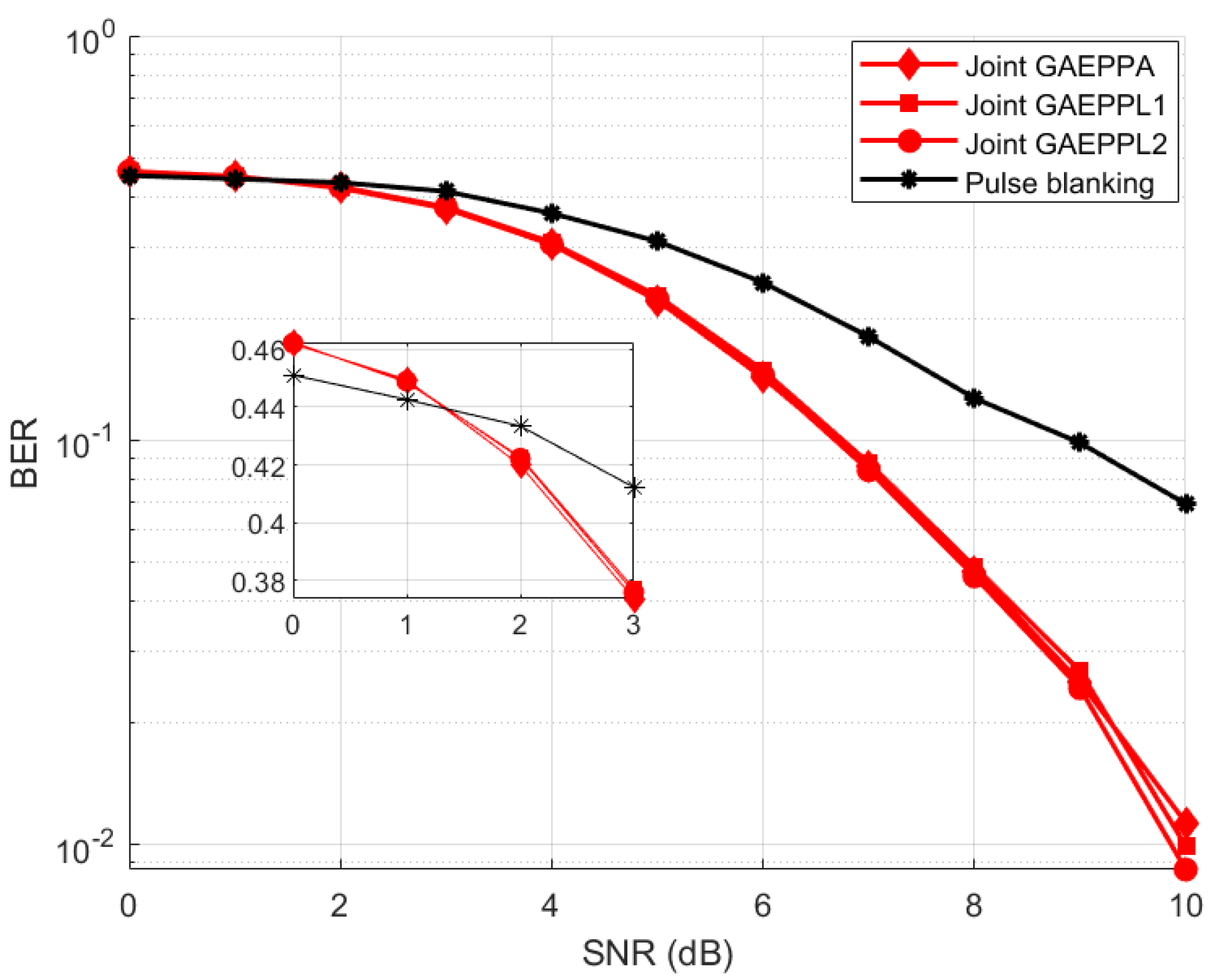
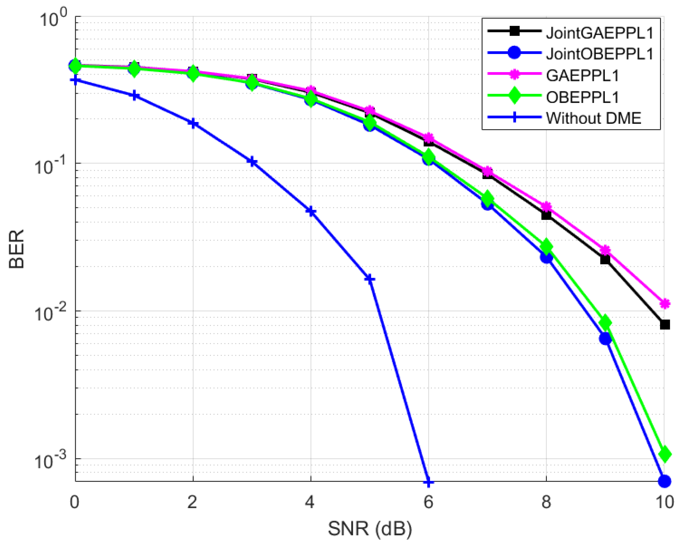
The DME mitigation of joint GAE enhanced PPA over a received data packet is better than GAE enhanced PPL or GAE enhanced PPA, which can be observed by comparing Figure 14 (right) with Figure 10 (right) and Figure 12 (right). The performance of joint GAE enhanced PPL is slightly better than joint GAE enhanced PPA, which can be verified from Figure 15.

The K-GMM modeling of the received signal is unavoidable for the accurate functioning of OBE. The proposed nonlinear estimators discussed in this paper utilize the statistical variables obtained from the 2-GMM modeling of complex valued received signal $y_t\left[n\right]$ resulting in two components with variances ${\sigma }_0^2$ and ${\sigma }_1^2$ and probability of occurrences $p_0$ and $p_1$. Figure 16a shows the absolute value of the OFDM data frame for all the ‘t’ values. Figure 16b,c shows the variance ${\sigma }_0^2$ and the corresponding probability $p_0$. Similarly, variance ${\sigma }_1^2$ and probability $p_1$ are displayed in Figure 16d and Figure 16e respectively. The numerical calculation of the scaling factor of OBE (${\beta }_o\left(y\right)$), which itself is a function of the received signal y is calculated from the statistical information (${\sigma }_0^2,{\sigma }_1^2$$p_0$ and $p_1$) obtained from 2-GMM modeling. Each term of this scaling factor is well explained in the system model.

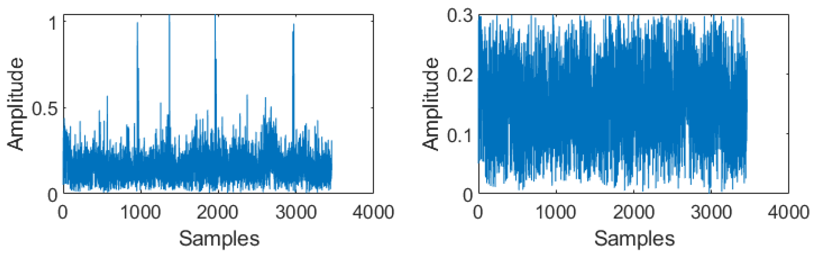
The value of ${\beta }_o\left(y\right)$ mathematically calculated from the statistical parameters obtained from the 2-GMM modeling is utilized in OBE in finding the Bayesian estimated value as in (23). Figure 17 (left) characterizes the CP removed OFDM data symbols in the time domain at the input of OBE, and Figure 17 (right) shows the corresponding optimum Bayesian estimated output. Careful observation of these two figures reveals the fact that though OBE could reduce the impulsive noise slightly, it is not sufficient to remove the DME noise. One of the possible reasons behind this could be the minimum value of K = 2, which is used to model the received complex data. Another reason could be the scaling of data in subcarriers that are not affected by impulse noise due to the minimum value of K used for Gaussian modeling. It may be possible to overcome these two reasons either by increasing the K value in K-GMM or by applying nonlinear scaling only to the noise-affected subcarriers. Considering the computational complexity that can be associated with higher values of K, we tried to obtain better performance from 2-GMM modeling. The second possibility gives way to the development of OBE enhanced PPA.

When the nonlinear scaling is applied only to selected subcarriers using (26), a reduction in BER could be achieved in comparison to pulse blanking as well as OBE. These results obtained are as displayed in Figure 18. Though the performance of OBE could be upgraded with the employment of OBE enhanced PPA, it is observed that attenuations applied to the affected subcarriers are not sufficient to eliminate the DME noise. It is evident from Figure 19. It may be possible to reduce BER even more, which leads to the development of OBE enhanced PPL.

OBE enhanced PPL performed nonlinear scaling only to the subcarriers which are affected with impulse noise in such a way that the amplitude of the resulting signal after nonlinear scaling is at least equal to the threshold value used for detecting the pulse peak (30). Comparing Figure 19 (right) and Figure 20 (right), we can clearly observe that the nonlinear output displays at Figure 20 (right) are the same as those in Figure 19 with the maximum output value limited to the threshold value used for identifying the affected subcarriers. As discussed in Section 4, this operation is possible in two ways, as in (28) and (29). It is observed that the results of both of these proposed methods are the same in reducing the BER rate at the output, as the same time difference in operation can be seen in Figure 21.

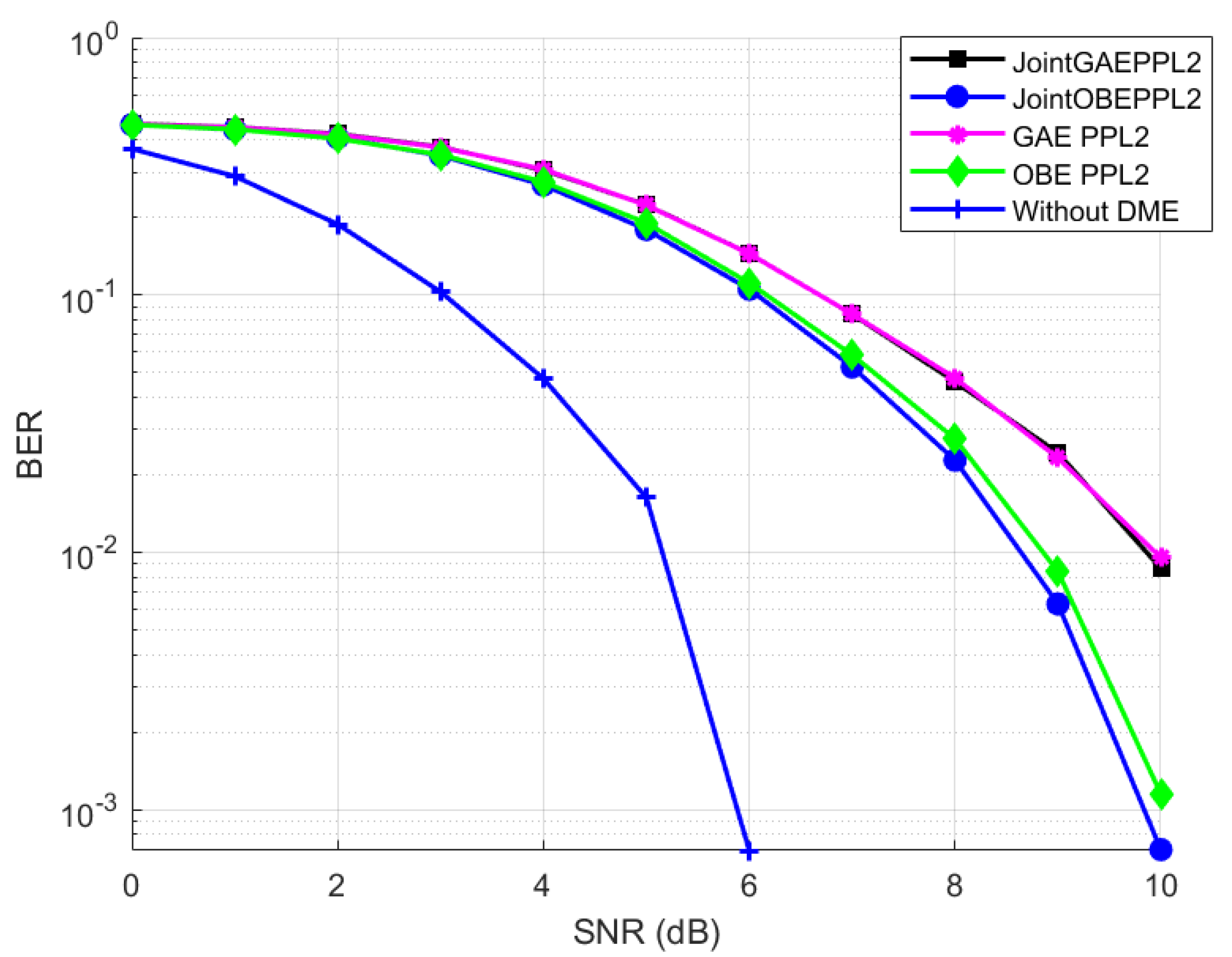
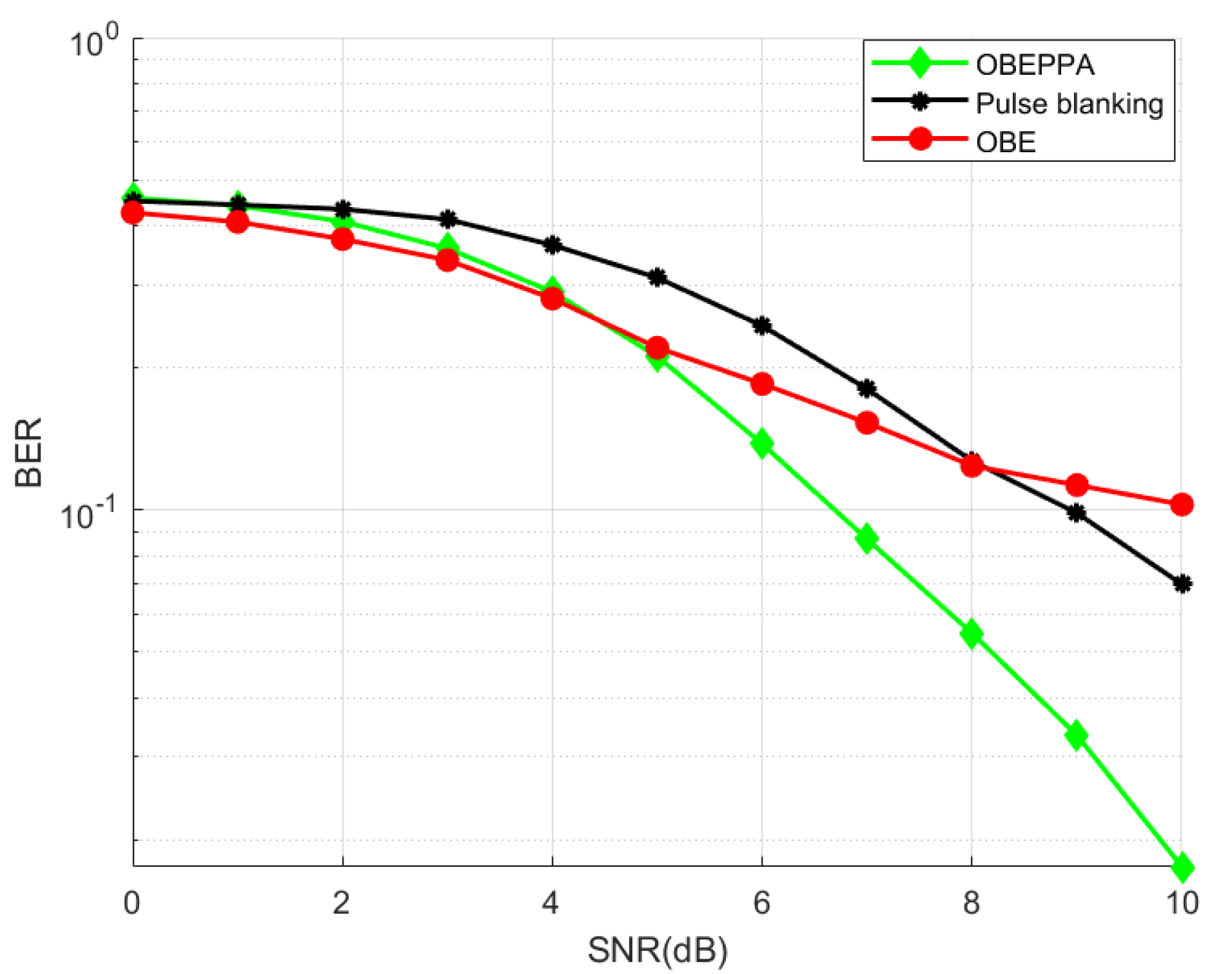
Further joint OBE enhanced PPA and joint OBE enhanced PPL showed almost similar performance, though the actual BER value differed slightly. Both of these methods showed a significant variation in reduction of BER at the receiver compared to the pulse blanking method, which is depicted in Figure 22. The operation of joint OBE enhanced PPA on OFDM signal is displayed in Figure 23. Finally, a performance comparison between all the proposed PPAs is shown in Figure 24. From this result, it is identified that JOBEPPA is the best method that could mitigate DME interference among all the proposed PPAs. 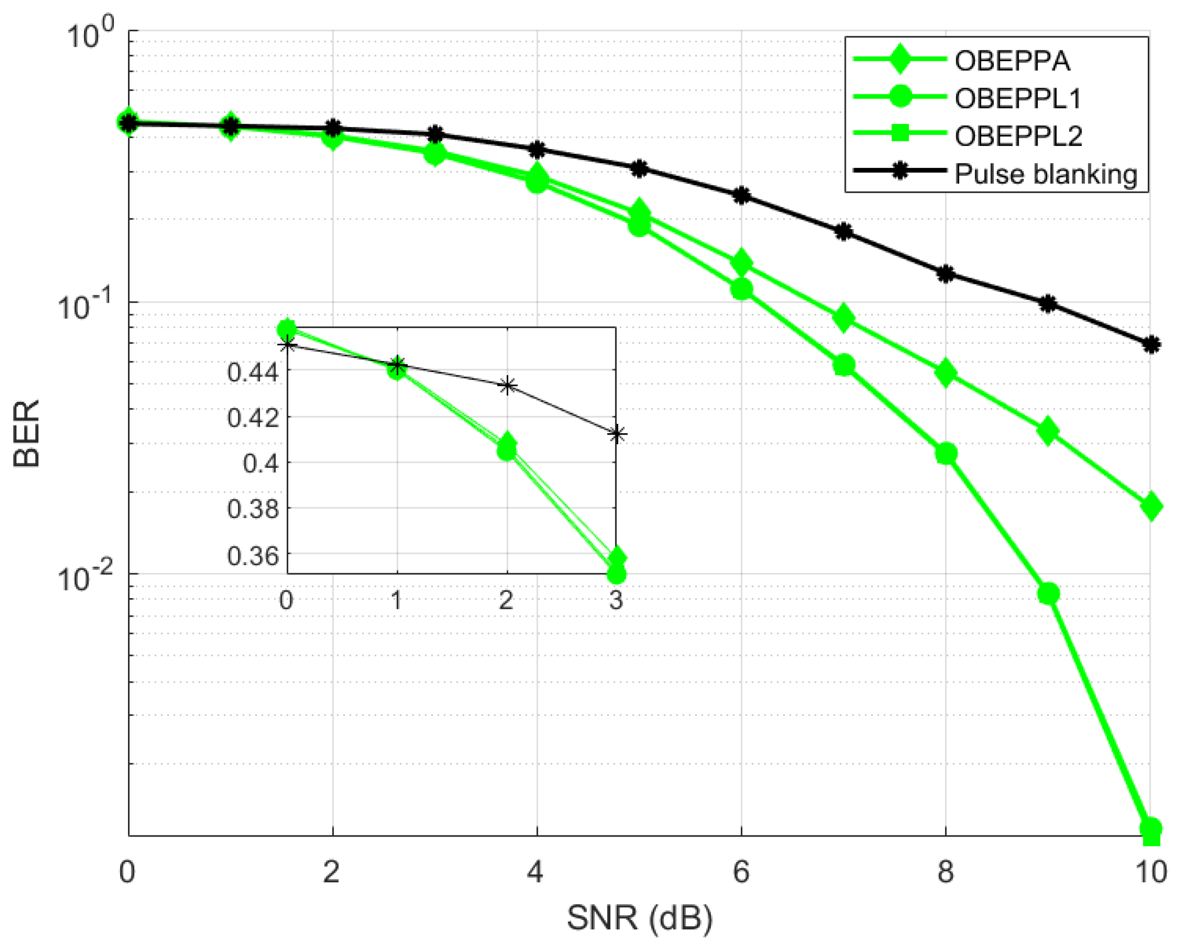Similarly, Figure 25 and Figure 26 show the comparison in different types of proposed PPLs. We can also observe that OBE enhanced methods outperformed the GAE enhanced methods, and this is expected from the literature survey.

6. Conclusions

In this article, different non-linear operations employing LDACS receiver architecture to mitigate the DME interference is proposed. With the knowledge of GAE and OBE, we propose simple yet improved pulse peak attenuators GAEPPA, OBEPPA, JGAEPPA and pulse peak limiters OBEPPA, OBEPPL, JOBEPPL. From the results obtained with the comparative study of these proposed methods along with the existing pulse blanking method, we observed the following:

1.

All these proposed methods exhibited improved performance compared to the pulse blanking method.

2.

OBE enhanced methods always outperformed GAE enhanced methods.

3.

Pulse peak limiters showed better performance than pulse peak attenuators in most of the cases. JOBEPPL and JOBEPPA showed almost similar performance as an exception, which in turn indicates the accuracy in estimation of JOBEPPA.

4.

Among all the proposed pulse peak attenuators, JOBE PPA had better received BER than JGAEPPA, OBEPPA and GAEPPA.

5.

Similarly, among all proposed PPLs, joint OBEPPL exhibited better performance than joint GAEPPL, OBEPPL and GAEPPL.

6.

JOBEPPL and JOBEPPA are the best nonlinear estimators within the proposed methods.

The SNR saving of joint OBEPPA and joint OBEPPL at ${10}^{-1}$ is around 3 dB. In the future, this work can be extended for en-route channel to address the issues discussed in [49] with suitable equalization techniques [50]. The performance of these methods in LDACS RL can be analyzed. Though these methods are investigated on the LDACS background, the methods are suitable in reducing impulse noise in any OFDM-based communication system.

References

1. EUROCONTROL. EUROCONTROL’s Challenges of Growth 2018 Study Report. Available online: https://www.eurocontrol.int/sites/default/files/2019-07/challenges-of-growth-2018-annex1-0.pdf (accessed on 29 September 2019).
2. Jacob, P.; Sirigina, R.P.; Madhukumar, A.S.; Prasad, V.A. Cognitive radio for aeronautical communications: A survey. IEEE Access 2016, 4, 3417–3443. [Google Scholar] [CrossRef]
3. Chiang, R.I.C.; Rowe, G.B.; Sower, K.W. A Quantitative Analysis of Spectral Occupancy Measurements for Cognitive Radio. In Proceedings of the 2007 IEEE 65th Vehicular Technology Conference—VTC2007, Dublin, Ireland, 22–25 April 2007; pp. 3016–3020. [Google Scholar] [CrossRef]
4. Wellens, M.; Wu, J.; Mahonen, P. Evaluation of Spectrum Occupancy in Indoor and Outdoor Scenario in the Context of Cognitive Radio. In Proceedings of the 2007 2nd International Conference on Cognitive Radio Oriented Wireless Networks and Communications, Orlando, FL, USA, 1–3 August 2007; pp. 420–427. [Google Scholar] [CrossRef]
5. Available online: https://www.ldacs.com/wp-content/uploads/2013/12/ACP-DCIWG-IP01-LDACS-White-Paper.pdf (accessed on 11 November 2021).
6. L-DACS1 System Defenition Proposal: Deliverable D2; Eurocontrol Study Rep.; Eur. Org. Safety Air Navigat.: Brussels, Belgium, 2009; Available online: https://www.ldacs.com/wp-content/uploads/2014/02/LDACS1-Specification-Proposal-D2-Deliverable.pdf (accessed on 11 November 2021).
7. L-DACS2 System Defenition Proposal: Delivrable D2; Tech. Rep. 1.0, Version 1; EUROCONTROL: Brussels, Belgium, 2009; Available online: https://www.eurocontrol.int/sites/default/files/2019-05/11052009-ldcas2-d2-deliverable-v1.0.pdf (accessed on 11 November 2021).
8. Epple, U.; Schnell, M. Mitigation of impulsive interference for LDACS1―Potentials of blanking nonlinearity. In Proceedings of the IEEE 2015 Integrated Communication, Navigation and Surveillance Conference (ICNS), Herndon, VA, USA, 21–23 April 2015; pp. 1–16. [Google Scholar]
9. Mostafa, M.; Schnell, M. DME-compliant LDACS1 cell planning: Initial steps. In Proceedings of the IEEE 2015 Integrated Communication, Navigation and Surveillance Conference (ICNS), Herndon, VA, USA, 21–23 April 2015; pp. 1–42. [Google Scholar]
10. Schnell, M.; Epple, U.; Shutin, D.; Schneckenburger, N.T. LDACS: Future aeronautical communications for air-traffic management. IEEE Commun. Mag. 2014, 52, 104–110. [Google Scholar] [CrossRef]
11. Thiasiriphet, T.; Schneckenburger, N.; Schnell, M. Impact of the DME interference on the LDACS1 ranging performance. In Proceedings of the 28th International Technical Meeting of the Satellite Division of the Institute of Navigation (ION GNSS+ 2015), Tampa, FL, USA, 14–18 September 2015; pp. 1446–1467. [Google Scholar]
12. Muthalagu, R.T. Mitigation of DME interference in LDACS1-based future air-to-ground (A/G) communications. Cogent Eng. 2018, 5, 1472199. [Google Scholar] [CrossRef]
13. Agrawal, N.; Darak, S.J. Performance analysis of reconfigurable filtered OFDM for LDACS. In Proceedings of the IEEE 2019 11th International Conference on Communication Systems & Networks (COMSNETS), Bengaluru, India, 7–11 January 2019; pp. 500–503. [Google Scholar]
14. Agrawal, N.; Darak, S.J.; Bader, F. Spectral Coexistence of LDACS and DME: Analysis via Hardware software co-design in presence of real channels and RF impairments. IEEE Trans. Veh. Technol. 2020, 69, 9837–9848. [Google Scholar] [CrossRef]
15. Agrawal, N.; Darak, S.J.; Bader, F.T. New Spectrum Efficient Reconfigurable Filtered-OFDM Based L-Band Digital Aeronautical Communication System. IEEE Trans. Aerosp. Electron. Syst. (TAES) 2019, 55, 1108–1122. [Google Scholar] [CrossRef] [Green Version]
16. Raja, M.T. Application of cognitive radio and interference cancellation in the L-Band based on future air-to-ground communication systems. Digit. Commun. Netw. 2019, 5, 111–120. [Google Scholar] [CrossRef]
17. Mathew, L.K.; Vinod, A.P. An energy-difference detection based spectrum sensing technique for improving the spectral efficiency of LDACS1 in aeronautical communications. In Proceedings of the 2016 IEEE/AIAA 35th Digital Avionics Systems Conference (DASC), Sacramento, CA, USA, 25–29 September 2016; pp. 1–5. [Google Scholar]
18. Mathew, L.K.; Vinod, A.P.; Madhukumar, A.S. A cyclic prefix assisted spectrum sensing method for aeronautical communication systems. In Proceedings of the 2019 IEEE International Symposium on Circuits and Systems (ISCAS), Sapporo, Japan, 26–29 May 2019; pp. 1–5. [Google Scholar]
19. Schneckenburger, N.; Franzen, N.; Gligorevic, S.; Schnell, M. L-band compatibility of LDACS1. In Proceedings of the 2011 IEEE/AIAA 30th Digital Avionics Systems Conference, Seattle, WA, USA, 16–20 October 2011. [Google Scholar]
20. Jain, R.; Templin, F.; Yin, K.S. Analysis of L-band digital aeronautical communication systems: L-DACS1 and L-DACS2. In Proceedings of the IEEE 2011 Aerospace Conference, Big Sky, MT, USA, 5–12 March 2011; pp. 1–10. [Google Scholar]
21. Epple, U.; Schnell, M. Overview of interference situation and mitigation techniques for LDACS1. In Proceedings of the 2011 IEEE/AIAA 30th Digital Avionics Systems Conference, Seattle, WA, USA, 16–20 October 2011. [Google Scholar]
22. Wang, H.; Liu, R. DME/TACAN interference mitigated by mixed blanking in B2 band. In Proceedings of the 2011 IEEE 13th International Conference on Communication Technology, Jinan, China, 25–28 September 2011; pp. 897–900. [Google Scholar]
23. Bai, Y.; Zhang, X.; Zhao, L. Co-channel CCK transmission overlapped with DME in aeronautical communication. In Proceedings of the 2014 IEEE China Summit & International Conference on Signal and Information Processing (ChinaSIP), Xi’an, China, 9–13 July 2014; pp. 403–406. [Google Scholar]
24. Li, Q.; Zhang, J.; Xie, J.; Mostafa, M.; Schnell, M. Iterative interference mitigation and channel estimation for LDACS1. In Proceedings of the 2014 IEEE/AIAA 33rd Digital Avionics Systems Conference (DASC), Colorado Springs, CO, USA, 5–9 October 2014. [Google Scholar]
25. Hirschbeck, M.; Huber, J.B. Block based frequency selective mitigation of pulsed interference in the L-band. In Proceedings of the 2015 10th International ITG Conference on Systems, Communications and Coding, Hamburg, Germany, 2–5 February 2015; pp. 1–6. [Google Scholar]
26. Li, D.; Wu, Z. DME Interference mitigation for L-DACS1 based on system identification and sparse representation. Chin. J. Aeronaut. 2016, 6, 1762–1773. [Google Scholar] [CrossRef] [Green Version]
27. Saaifan, K.A.; Henkel, W. Lattice signal sets to combat pulsed interference from aeronautical signals. In Proceedings of the 2011 IEEE International Conference on Communications (ICC), Kyoto, Japan, 5–9 June 2011; pp. 1–5. [Google Scholar]
28. Abd-Elaty, E.; El-Agooz, S.; Zekry, A.E. Compact Spread Spectrum LDACS Wavelet Based for DME Interference Mitigation. In Proceedings of the IEEE 2019 36th National Radio Science Conference (NRSC), Port Said, Egypt, 16–18 April 2019; pp. 259–265. [Google Scholar]
29. Miziya, K.; Muthalagu, R.; Mathew, L.K.; Rajak, A. Deep Clipping Based Interference Mitigation Technique for LDACS. In Proceedings of the 2021 IEEE/AIAA 40th Digital Avionics Systems Conference (DASC), San Antonio, TX, USA, 3–7 October 2021; pp. 1–6. [Google Scholar] [CrossRef]
30. Darsena, D.; Gelli, G.; Melito, F.; Verde, F. ICI-Free Equalization in OFDM Systems with Blanking Preprocessing at the Receiver for Impulsive Noise Mitigation. IEEE Signal Process. Lett. 2015, 22, 1321–1325. [Google Scholar] [CrossRef] [Green Version]
31. Eriksson, H.B.; Ödling, P.; Koski, T.; Börjesson, P.O. A genie-aided detector with a probabilistic description of the side information. Proceedings of 1995 IEEE International Symposium on Information Theory, Whistler, BC, Canada, 17–22 September 1995; p. 332. [Google Scholar] [CrossRef] [Green Version]
32. Rožić, N.; Banelli, P.; Begušić, D.; Radić, J. Multiple-Threshold Estimators for Impulsive Noise Suppression in Multicarrier Communications. IEEE Trans. Signal Process. 2018, 10, 1619–1633. [Google Scholar] [CrossRef]
33. Banelli, P. Bayesian estimation of a Gaussian source in Middleton’s class—A impulsive noise. IEEE Signal Process. Lett. 2013, 20, 956–959. [Google Scholar] [CrossRef] [Green Version]
34. Banelli, P.; Rugini, L. Impulsive noise mitigation for wireless OFDM. In Proceedings of the 2015 IEEE 16th International Workshop on Signal Processing Advances in Wireless Communications (SPAWC), Stockholm, Sweden, 28 June–1 July 2015; pp. 346–350. [Google Scholar]
35. Gao, G.X. DME/TACAN Interference and its Mitigation in L5/E5 Bands. In Proceedings of the 20th International Technical Meeting of the Satellite Division of the Institute of Navigation (ION GNSS 2007), Fort Worth, TX, USA, 25–28 September 2007; pp. 1191–1200. [Google Scholar]
36. Kassam, S.A. Signal Detection in Non-Gaussian Noise; Springer Science & Business Media: New York, NY, USA, 1988. [Google Scholar]
37. Barazideh, R.; Natarajan, B.; Nikitin, A.V.; Niknam, S.T. Performance Analysis of Analog Intermittently Nonlinear Filter in the Presence of Impulsive Noise. IEEE Trans. Veh. Technol. 2019, 68, 3565–3573. [Google Scholar] [CrossRef]
38. Sanchez, M.G.; De Haro, L.; Ramón, M.C.; Mansilla, A.; Ortega, C.M.; Oliver, D.T. Impulsive noise measurements and characterization in a UHF digital TV channel. IEEE Trans. Electromagn. Compat. 1999, 41, 124–136. [Google Scholar] [CrossRef]
39. Blackard, K.L.; Rappaport, T.S.; Bostian, C.W. Measurements and models of radio frequency impulsive noise for indoor wireless communications. IEEE J. Sel. Areas Commun. 1993, 10, 991–1001. [Google Scholar] [CrossRef] [Green Version]
40. Nakai, T.; Kawasaki, Z.T. On impulsive noise from Shinkansen. IEEE Trans. Electromagn. Compat. 1983, 4, 396–404. [Google Scholar] [CrossRef]
41. Dempster, A.P.; Laird, N.M.; Rubin, D.B. Maximum likelihood from incomplete data via the EM algorithm. J. R. Stat. Soc. Ser. B (Methodol.) 1977, 39, 1–22. [Google Scholar]
42. Al-Naffouri, T.Y.; Quadeer, A.A.; Caire, G. Impulse noise estimation and removal for OFDM systems. IEEE Trans. Commun. 2014, 62, 976–989. [Google Scholar] [CrossRef]
43. Hur, S.; Baek, S.; Kim, B.; Chang, Y.; Molisch, A.F.; Rappaport, T.S.; Haneda, K.; Park, J. The title of the cited article. J. Abbr. 2008, 10, 142–149. [Google Scholar]
44. Zhidkov, S.V. Performance analysis and optimization of OFDM receiver with blanking nonlinearity in impulsive noise environment. IEEE Trans. Veh. Technol. 2006, 55, 234–242. [Google Scholar] [CrossRef]
45. Alam, M.S.; Kaddoum, G.; Agba, B.J.; Bayesian, L. MMSE Estimation of a Gaussian Source in the Presence of Bursty Impulsive Noise. IEEE Commun. Lett. 2018, 22, 1846–1849. [Google Scholar] [CrossRef]
46. ALin, J.; Nassar, M.; Evans, B.L. Impulsive noise mitigation in powerline communications using sparse Bayesian learning. IEEE J. Sel. Areas Commun. 2013, 31, 1172–1183. [Google Scholar]
47. Middleton, D. Threshold detection in correlated non-Gaussian noise fields. IEEE Trans. Inf. Theory 1995, 41, 976–1000. [Google Scholar] [CrossRef]
48. Sadler, B.M. Detection in correlated impulsive noise using fourth-order cumulants. IEEE Trans. Signal Process 1996, 44, 2793–2800. [Google Scholar] [CrossRef]
49. Haas, E.T. Aeronautical channel modeling. IEEE Trans. Veh. Technol. 2002, 51, 254–264. [Google Scholar] [CrossRef]
50. Darsena, D.; Gelli, G.; Iudice, I.; Verde, F. Equalization Techniques of Control and Non-Payload Communication Links for Unmanned Aerial Vehicles. IEEE Access 2018, 4485–4496. [Google Scholar] [CrossRef]
Figure 1. L-Band spectrum occupancy [12].
Aerospace 09 00045 g001
Figure 2. Interference between DME and LDACS [16].
Aerospace 09 00045 g002
Figure 3. LDACS transmitter block diagram.
Aerospace 09 00045 g003
Figure 4. Proposed LDACS receiver block diagram.
Aerospace 09 00045 g004
Figure 5. General block diagram for GAE and OBE.
Aerospace 09 00045 g005
Figure 6. General block diagram for pulsepeak processors.
Aerospace 09 00045 g006
Figure 7. Performance of conventional pulse blanking technique vs. without DME interference and with DME interference.
Aerospace 09 00045 g007
Figure 8. (left) Absolute values of received OFDM data frame. (right) Variance k obtained from the 2-GMM of data.
Aerospace 09 00045 g008
Figure 9. (left) OFDM data at the receiver along with DME interference and AWGN noise. (right) Output of genie-aided estimator in the time domain.
Aerospace 09 00045 g009
Figure 10. (left) OFDM data at the receiver along with DME interference and AWGN noise. (right) Output of GAEPPA in the time domain.
Aerospace 09 00045 g010
Figure 11. Performance comparison of the proposed GAE enhanced PPA vs. the conventional pulse blanking and GAE.
Aerospace 09 00045 g011
Figure 12. (left) OFDM data at the receiver along with DME interference and AWGN noise. (right) Output of GAEPPL in the time domain.
Aerospace 09 00045 g012
Figure 13. Performance comparison of the proposed GAEPPA, GAEPPL1 and GAEPPL2 vs. the conventional pulse blanking.
Aerospace 09 00045 g013
Figure 14. (left) OFDM data at the receiver along with DME interference and AWGN noise. (right) Output of joint GAEPPA in the time domain.
Aerospace 09 00045 g014
Figure 15. Performance comparison of the proposed joint GAEPPA, joint GAEPPL1 and joint GAEPPL2 vs. the conventional pulse blanking.
Aerospace 09 00045 g015
Figure 16. (a) Absolute value of received OFDM data after CP removal. (b) Variance zero. (c) Probability of occurrence variance zero. (d) Variance 1. (e) Probability of occurrence variance one.
Aerospace 09 00045 g016
Figure 17. (left) Received data packet along with DME and AWGN noise. (right) Output of OBE in the time domain.
Aerospace 09 00045 g017
Figure 18. Performance comparison of proposed method OBE enhanced PPA with conventional pulse blanking technique and OBE.
Aerospace 09 00045 g018
Figure 19. (left) Received data packet along with DME and AWGN noise. (right) Output of OBEPPA in the time domain.
Aerospace 09 00045 g019
Figure 20. (left) Received data packet along with DME and AWGN noise. (right) Output of OBE PPL in the time domain.
Aerospace 09 00045 g020
Figure 21. Performance comparison of proposed methods OBE enhanced PPL and OBE enhanced PPL1 and PPL2 with conventional pulse blanking technique.
Aerospace 09 00045 g021
Figure 22. Performance comparison of the proposed joint OBEPPA, joint OBEPPL1 and joint OBEPPL2 vs. the conventional pulse blanking.
Aerospace 09 00045 g022
Figure 23. (left) Received data packet along with DME and AWGN noise. (right) Output of joint OBEPPA in the time domain.
Aerospace 09 00045 g023
Figure 24. Performance comparison of proposed four types of pulse peak attenuators.
Aerospace 09 00045 g024
Figure 25. Performance comparison of proposed four types of pulse peak Type 1 limiters.
Aerospace 09 00045 g025
Figure 26. Performance comparison of proposed four types of pulse peak Type 2 limiters.
Aerospace 09 00045 g026