Incomplete Information Pursuit-Evasion Game Control for a Space Non-Cooperative Target

Abstract

Aiming to solve the optimal control problem for the pursuit-evasion game with a space non-cooperative target under the condition of incomplete information, a new method degenerating the game into a strong tracking problem is proposed, where the unknown target maneuver is processed as colored noise. First, the relative motion is modeled in the rotating local vertical local horizontal (LVLH) frame originated at a virtual Chief based on the Hill-Clohessy-Wiltshire relative dynamics, while the measurement models for three different sensor schemes (i.e., single LOS (line-of-sight) sensor, LOS range sensor and double LOS sensor) are established and an extended Kalman Filter (EKF) is used to obtain the relative state of target. Next, under the assumption that the unknown maneuver of the target is colored noise, the game control law of chaser is derived based on the linear quadratic differential game theory. Furthermore, the optimal control law considering the thrust limitation is obtained. After that, the observability of the relative orbit state is analyzed, where the relative orbit is weakly observable in a short period of time in the case of only LOS angle measurements, fully observable in the cases of LOS range and double LOS measurement schemes. Finally, numerical simulations are conducted to verify the proposed method. The results show that by using the single LOS scheme, the chaser would firstly approach the target but then would lose the game because of the existence of the target’s unknown maneuver. Conversely, the chaser can successfully win the game in the cases of LOS range and double LOS sensor schemes.

1. Introduction

With the progress of human space exploration, the number of space debris and inactive satellites has been increasing sharply, which has become a significant threat to active spacecraft and satellites; thus, cleaning up these space debris has become an important issue. Furthermore, along with the development of space rendezvous and docking technology [1,2], non-cooperative target observation [3] and approaching technics [4], the safety of space assets is threatened more than ever by military vehicles. Therefore, protecting the safety of space assets in face of these threats is critical for cleaning space. Many studies have been done to find a way out, e.g., space situational awareness, on-orbit servicing and so on [5,6,7,8,9,10,11,12]. Developing on-orbit servicing vehicles with corresponding GNC (guidance, navigation and control) systems used to handle the space debris, inactive satellites and military vehicles threating to the space asset is the most effective method for safety. In this manuscript, the topic of pursuit-evasion game control, as a further problem of space rendezvous for space non-cooperative target, will be studied.

ISAACS [13] has the earliest study for differential games, and gave the optimal necessary conditions for pursuit-evasion games. In 1971, Friedman [14] established the theory of differential game value and saddle point existence using the discrete approximate sequence, which laid a solid mathematical foundation in the differential game. Starr and Ho [15] studied the nonzero-sum N-person differential game of three different types. Roxin and Tsokos [16] gave the mathematical definition of stochastic differential game, Nichols [17] pointed out the relationship between the stochastic differential game and cybernetics and Ciletti [18,19,20,21] studied the differential game containing information delay, and established the open loop and closed loop control of the information delay differential game. In the 1980s, Stackelberg’s [22] master-slave differential game become the new hotspot among many scholars in the 1990s. Since 2000, differential game research has mainly concentrated on the zero-sum with state constraints and the differential game, many differential game and incomplete information differential pairs.

Aumann and Maschler [23] and Harsanyi [24] studied static incomplete information differential countermeasures, where Harsanyi converted the game with incomplete information into a complete but imperfect game, and used the methods for processing full information. Kreps and Wilson [25] studied the dynamic incomplete information differential countermeasures, introducing the perfect Bayesian balance, sequential balance, etc. to introduce discrete dynamic games. The basis and conditions for making decisions for non-cooperative targets are unable to understand that the relevant relative state information of the other party may not be obtained in the incomplete information game. For the first problem mentioned above, Woodbury and Hurtado proposed adaptive control policies [26] that obtain the weight of the target function of the other party by order, which is not applicable to the unknown target function form; for the latter problem mentioned above, they proposed a method of adding an additional spacecraft for observation to obtain location information of the target [27]. Cavalieri further studied the incomplete information game in uncertain relative kinetics situation by joining the problem of the incomplete information game [28] with further studies of the incomplete information game in uncertain relative kinetics [29], that is, joining an estimate on the basis of the behavioral learning algorithm. Woodbury used similar methods [30]. Since the learning algorithm requires strong on-board calculation capabilities, Liu et al. built a fuzzy reasoning model to characterize continuous space, and proposed a branch depth strengthening learning architecture with multiple sets of parallel neural networks and shared decision modules [31]. Linville used the linear regression model [32] for incomplete information game to improve the practicality of the depth learning algorithm. DONG et al. proposed a multi-mode adaptive solution to the incomplete information game [33]. Similarly, Li studied the incomplete information game by estimating and modifying the guess of target’s control strategy constantly [34].

As an important case of incomplete information, bearings-only measurements have been widely studied. Oshman and Davidson proposed a method which is based on maximizing the determinant of the Fisher information matrix (FIM) to design the optimal observation trajectory for observer [35]. Battistini and Shima proposed a new guidance strategy that exploits the information from the error covariance matrix of the homing loop integrated Kalman filter in the framework of a pursuit-evasion game for missile [36]. Fonod and Shima studied cooperative estimation/guidance for a team of missiles by using bearings-only measurements [37]. Battistini presented a method for characterizing the capture region of a pursuit-evasion game in terms of the confidence on the estimation of the ZEM [38].

In summary, the pursuit-evasion game problem in the complicated space environment is quite challenging, especially in the case of incomplete feedback information. The main contribution of this research is to develop the space pursuit-evasion game control algorithm in the context of incomplete feedback information, i.e., angles-only measurements and known target maneuvers. Unlike previous researches estimating the unknown maneuvers by over-burden calculated artificial intelligent approach, the proposed algorithm in this paper treats it as colored noise, while a double line-of-sight scheme is developed to overcome the problems of the colored noise and observability resulting from angles-only measurements. It can potentially provide a feasible solution to the space game problem.

The rest of the paper is organized as follows. The relative motion dynamics for the game participants are presented in Section 2. The measurements models for three observation schemes are established in Section 3, followed by the observability analysis for the states in Section 4. The basic theory of the differential game control of pursuit-evasion is reviewed in Section 5. The space pursuit-evasion game control algorithm based on incomplete information is designed in Section 6. Numerical simulations with performance index and simulation parameters are set in Section 7. Conclusions are presented in Section 8.

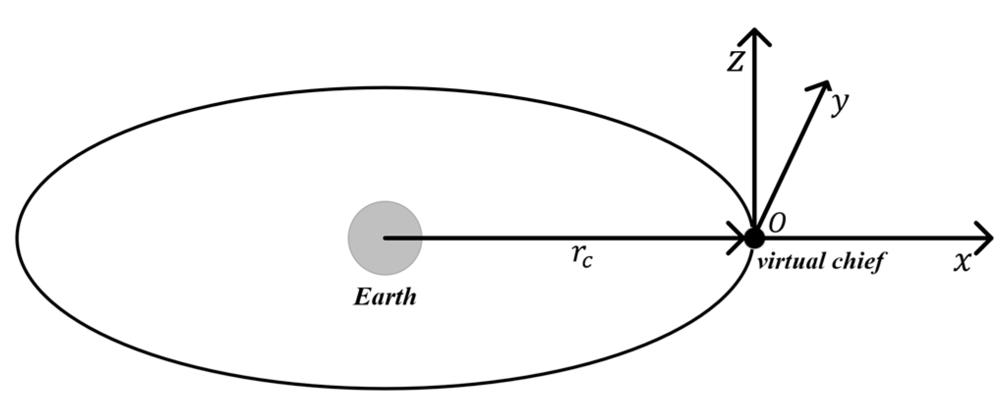
2. Relative Dynamics Model

Two participants in a two-player spacecraft pursuit-evasion (PE) game are called Pursuer and Evader, respectively. Typically, the objective of the Pursuer is to intercept/rendezvous with the Evader and the objective of the Evader is to avoid or delay the interception/rendezvous. To descript the pursuit-evasion game between Pursuer and Evader, a rotating local vertical local horizontal (LVLH) reference frame is adopted. The origin of the LVLH frame is collocated with a virtual Chief, as shown in Figure 1, where the axes are aligned with the inertial position vector (x axis or radial), the normal to orbit plane (z axis or cross track) and the along-track direction (y axis completes the orthogonal set). Let the relative orbit state be $x={[r^T,v^T]}^T$, where the superscript T stands for the operator of transposition. Vectors without a superscript are assumed to be coordinated in LVLH frames.

Then, under the assumptions of near-circular orbit, the two-body problem and that the range between the virtual Chief and the participants in the game is relatively small compared to the radial distance to the center of the Earth, the relative motion of the participants with respect to the virtual Chief can be governed by the well-known Hill-Clohessy-Wiltshire (HCW) equation [39]:

$$\{\begin{array}{c}{\dot{\mathit{x}}}_p=\mathit{A}{\mathit{x}}_p+\mathit{B}{\mathit{u}}_p\\ {\dot{\mathit{x}}}_e=\mathit{A}{\mathit{x}}_e+\mathit{B}{\mathit{u}}_e\end{array}$$

(1)

$$\mathit{A}=\left[\begin{array}{cccccc}0& 0& 0& 1& 0& 0\\ 0& 0& 0& 0& 1& 0\\ 0& 0& 0& 0& 0& 1\\ 3n^2& 0& 0& 0& 2n& 0\\ 0& 0& 0& -2n& 0& 0\\ 0& 0& -n^2& 0& 0& 0\end{array}\right]$$

(2)

$$\mathit{B}=\left[\begin{array}{c}{\mathit{0}}_{3\times 3}\\ {\mathit{I}}_{3\times 3}\end{array}\right]$$

(3)

where the subscripts of $p$ and $e$ stand for Pursuer and Evader, respectively, $n$ is the orbital rate of the virtual chief and $\mathit{u}$ is the control acceleration, which is loaded on the participants along the three axes of LVLH frame.

Then, let the relative state of Evader relative to Pursuer be $\mathit{x}={\mathit{x}}_e-{\mathit{x}}_p$ in the defined LVLH frame, which can be obtained from Equation (1) as follows:

$$\dot{\mathit{x}}=\mathit{A}\mathit{x}+{\mathit{B}}_p{\mathit{u}}_p+{\mathit{B}}_e{\mathit{u}}_e$$

(4)

where ${\mathit{B}}_p=-\mathit{B}$, ${\mathit{B}}_e=\mathit{B}$.

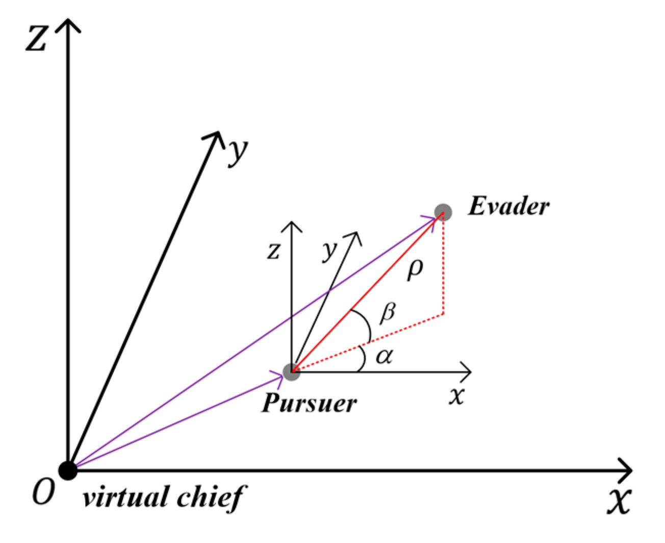
3. Measurement Models

The relative motion geometry between the Evader and Pursuer in the LVLH frame is shown in Figure 2, where the measurements observed by the Pursuer are generally assumed to be the line-of-sight (LOS) angles and relative range. Three observation schemes, i.e., single LOS sensor, LOS range sensor and double LOS sensors, are discussed in the following sections.

3.1. Single LOS Sensor Measurement

When the LOS angles are measured from only one passive camera available for the Pursuer, the observation can be modeled as follows:

$$\mathit{Z}=\left[\begin{array}{c}\alpha \\ \beta \end{array}\right]=\left[\begin{array}{c}\arctan (\frac{y}{x})\\ \arctan (\frac{z}{\sqrt{x^2+y^2}})\end{array}\right]$$

(5)

where $\alpha$ and $\beta$ are the azimuth and pitch angle, respectively.

3.2. LOS Range Sensor Measurement

With the active sensor such as radar/lidar on board, both of the LOS angles and range can be measured. Then, the observation model can be governed as follows:

$$\mathit{Z}=\left[\begin{array}{c}\alpha \\ \beta \\ \rho \end{array}\right]=\left[\begin{array}{c}\arctan (\frac{y}{x})\\ \arctan (\frac{z}{\sqrt{x^2+y^2}})\\ \sqrt{x^2+y^2+z^2}\end{array}\right]$$

(6)

where $\rho$ refers to the distance between the Pursuer and Evader.

3.3. Double LOS Sensor Measurement

When two or more passive optical sensors (e.g., two cameras) can be used to measure the LOS, as shown in Figure 3, the observation model can be given as follows:

$$\mathit{Z}=\left[\begin{array}{c}{\alpha }_1\\ {\beta }_1\\ \begin{array}{c}{\alpha }_2\\ {\beta }_2\end{array}\\ \mathit{R}\end{array}\right]=\left[\begin{array}{c}\arctan (\frac{y_1}{x_1})\\ \arctan (\frac{z_1}{\sqrt{x_1^2+y_1^2}})\\ \arctan (\frac{y_2}{x_2})\\ \arctan (\frac{z_2}{\sqrt{x_2^2+y_2^2}})\\ x_1-x_2\\ y_1-y_2\\ z_1-z_2\end{array}\right]$$

(7)

where the subscripts 1 and 2 are the label of sensors, ${\left[\begin{array}{ccc}{x}_1& y_1& z_1\end{array}\right]}^T$ and ${\left[\begin{array}{ccc}{x}_2& y_2& z_2\end{array}\right]}^T$ stand for the relative position from the Evader to the cameras, respectively, and the vector $\mathit{R}$ represents the baseline between two cameras, which is supposed to be known and can be calculated from the locations of the cameras.

Accordingly, when the observation model shown in Equation (7) is used, the system state $\mathit{X}$ for the estimation can be switched to a 12-dimension vector as follows:

$$\mathit{X}={\left[\begin{array}{cc}{\mathit{x}}_{e1}& {\mathit{x}}_{e2}\end{array}\right]}^T$$

(8)

where ${\mathit{x}}_{e1}$ and ${\mathit{x}}_{e2}$ refer to the state of the Evader as related to the cameras of the Pursuer.

4. Observability Analysis

Conceptually, the system is observable if the relative state can be uniquely determined from the measurements in time history. By contrast, the system is unobservable if more than one set of states share the same measurements in time history. The goal of this section is to mathematically analyze the observability of the system for the three utilized measurement modes based on the method presented in Ref. [2].

4.1. Observability Analysis in the Case of Single LOS Sensor Measurement

The observation equations can be conducted through a transformation in the form of “Analogous Linearization” [40]. Taking the tangent of the LOS angles $\alpha$ and $\beta$ in Equation (5) and simplifying yields:

$$\left[\begin{array}{c}x\sin (\alpha )-y\cos (\alpha )\\ y\sin (\beta )-z\sin (\alpha )\cos (\beta )\end{array}\right]=\mathbf{0}$$

(9)

By reorganizing Equation (9), a homogeneous linear equation is obtained:

$${\mathit{h}}_A(Z)x=\mathbf{0}$$

(10)

where:

$${\mathit{h}}_A(Z)=\left[\begin{array}{ccc}\sin (\alpha )& -\cos (\alpha )& 0\\ 0& \sin (\beta )& -\sin (\alpha )\cos (\beta )\end{array}|{\mathbf{0}}_{2\times 3}\right]$$

(11)

Obviously, the rank of ${\mathit{h}}_A(Z)$ is 2. Then, the 6-dimension state $x$ cannot be uniquely solved. Theoretically, at least three sets of measurements are required for solving $x$ uniquely. Then, if there are three sets of measurements, the following linear equations can be obtained:

$$\{\begin{array}{c}{\mathit{h}}_A(Z_0)x_0=\mathbf{0}\\ {\mathit{h}}_A(Z_1)x_1=\mathbf{0}\\ {\mathit{h}}_A(Z_2)x_2=\mathbf{0}\end{array}$$

(12)

where $x_0$ is the initial relative state. The state $x_k$ on epoch $t_k$ can be obtained from state transition equation, which is derived from the solution of the HCW equation, as follows:

$$x_k=\mathit{\varphi }{x}_{k-1}+G{u}_{k-1}+{\mathit{\omega }}_{k-1}$$

(13)

where $\mathit{\varphi }$ is the state transition matrix, $G$ is the control driven matrix, and ${\mathit{\omega }}_{k-1}$ is noise which originates from the maneuver of Evader and error of the HCW equation.

Substituting Equation (13) into Equation (12) and reforming the equation produces gives the following:

$$\left[\begin{array}{c}{\mathit{h}}_A(Z_0)\\ {\mathit{h}}_A(Z_1)\mathit{\varphi }\\ {\mathit{h}}_A(Z_2){\mathit{\varphi }}^2\end{array}\right]x_0=-\left[\begin{array}{c}\mathbf{0}\\ {\mathit{h}}_A(Z_1)(G{u}_0+{\mathit{\omega }}_0)\\ {\mathit{h}}_A(Z_2)(\mathit{\varphi }(G{u}_0+{\mathit{\omega }}_0)+G{u}_1+{\mathit{\omega }}_1)\end{array}\right]$$

(14)

Equation (14) is a non-homogeneous linear equation if the maneuver of Pursuer is non-zero, where the control vector of Pursuer $u$ is non-linear function of state vector $\mathit{x}$. Then, the initial relative state vector can be solved when ${\mathit{\omega }}_{k-1}$ is known, so the system is observable if the maneuver of the Evader is known. However, the colored noise ${\mathit{\omega }}_{k-1}$ (the Evader’s maneuver) is unknown, so even if the system is observable, the solution would be polluted, which decreases the accuracy of the solution.

4.2. Observability Analysis with the LOS Range Measurement

When the distance measurement is added to the observation, the relative position of the Evader can be calculated by the following equation:

$$r=\rho \left[\begin{array}{c}\cos (\alpha )\cos (\beta )\\ \cos (\alpha )\sin (\beta )\\ \sin (\alpha )\end{array}\right]$$

(15)

Thus, the converted observation is:

$${\mathit{h}}_r({\mathit{Z}}_k)={\mathit{r}}_k=\mathit{C}{\mathit{x}}_k$$

(16)

where:

$$\mathit{C}={\left[\begin{array}{cc}\mathit{I}& \mathit{0}\end{array}\right]}_{3\times 6}$$

(17)

$${\mathit{h}}_r(\mathit{Z})=\rho \left[\begin{array}{c}\cos (\alpha )\cos (\beta )\\ \cos (\alpha )\sin (\beta )\\ \sin (\alpha )\end{array}\right]$$

(18)

Similarly, the rank of ${\mathit{h}}_r(\mathit{Z})$ is 3 and the dimension of state $x$ is 6, so at least two sets of measurements are required for solution of state $x$. Then, based on Equation (13) and Equation (16), the following equation can be obtained:

$$\left[\begin{array}{c}\mathit{C}\\ \mathit{C}\mathit{\varphi }\end{array}\right]{\mathit{x}}_0=\left[\begin{array}{c}{\mathit{h}}_r({\mathit{Z}}_0)\\ {\mathit{h}}_r({\mathit{Z}}_1)-\mathit{C}(\mathit{G}{\mathit{u}}_0+{\mathit{\omega }}_0)\end{array}\right]$$

(19)

Equation (19) is a non-homogeneous linear equation, and the system is observable if the maneuver of the Evader is known. Different from the single LOS sensor measurement case, Equation (19) has the component ${\left[\begin{array}{cc}{\mathit{h}}_r{}^T({\mathit{Z}}_0)& {\mathit{h}}_r{}^T({\mathit{Z}}_1)\end{array}\right]}^T$, which means that the filter is more stable in the case of joint measurement with LOS and range sensors.

4.3. Observability Analysis with Double LOS Measurements

When the binocular camera is used, the observation model of Equation (7) can be used. Similar to the observability analysis of a single camera measurement, the following equation can be obtained:

$$\left[\begin{array}{cc}{\mathit{h}}_A({\alpha }_1,{\beta }_1)& {\mathit{0}}_{2\times 6}\\ {\mathit{0}}_{2\times 6}& {\mathit{h}}_A({\alpha }_2,{\beta }_2)\\ \begin{array}{cc}{\mathit{I}}_{3\times 3}& {\mathit{0}}_{3\times 3}\end{array}& \begin{array}{cc}-{\mathit{I}}_{3\times 3}& {\mathit{0}}_{3\times 3}\end{array}\end{array}\right]\mathit{X}=\left[\begin{array}{c}{\mathit{0}}_{4\times 1}\\ \mathit{R}\end{array}\right]$$

(20)

Equation (20) can be written in the following form:

$${\mathit{H}}_{DA}(\mathit{Z})\mathit{X}=\left[\begin{array}{c}{\mathit{0}}_{4\times 1}\\ \mathit{R}\end{array}\right]$$

(21)

where the rank of ${\mathit{H}}_{DA}(\mathit{Z})$ is 6; thus, $\mathit{X}$ cannot be determined uniquely from Equation (21). The state transfer equation of $\mathit{X}$ can be obtained by Equation (13) in the following form:

$${\mathit{X}}_k=\mathit{\Phi }{\mathit{X}}_{k-1}+{\mathit{Y}}_{k-1}$$

(22)

where:

$$\mathit{\Phi }=\left[\begin{array}{cc}\mathit{\varphi }& \mathit{0}\\ \mathit{0}& \mathit{\varphi }\end{array}\right]$$

(23)

$${\mathit{Y}}_{k-1}=\left[\begin{array}{c}\mathit{G}{\mathit{u}}_{k-1}\\ \mathit{G}{\mathit{u}}_{k-1}\end{array}\right]+(\mathit{\Phi }-\mathit{I})\left[\begin{array}{c}{\mathit{R}}_1\\ {\mathit{0}}_{3\times 1}\\ {\mathit{R}}_2\\ {\mathit{0}}_{3\times 1}\end{array}\right]$$

(24)

Based on Equations (21) and (22), the following equation can be obtained when two sets of measurements are available:

$$\left[\begin{array}{c}{\mathit{H}}_{DA}({\mathit{Z}}_0)\\ {\mathit{H}}_{DA}({\mathit{Z}}_1)\mathit{\Phi }\end{array}\right]{\mathit{X}}_0=\left[\begin{array}{c}{\mathit{0}}_{4\times 1}\\ \mathit{R}\\ {\mathit{0}}_{4\times 1}\\ \mathit{R}\end{array}\right]-\left[\begin{array}{c}{\mathit{0}}_{7\times 1}\\ {\mathit{H}}_{DA}({\mathit{Z}}_1){\mathit{Y}}_0\end{array}\right]$$

(25)

Under the measurement of double LOS sensors, the filter has strong convergent performance with the measurement component made up of $\mathit{R}$, ${\mathit{R}}_1$, and ${\mathit{R}}_2$, and the system still has observability with limited colored noise. Compared to the above two measurement methods,

Table 1. Comparison of the above three measurement methods.

Observability	Single LOS	LOS Range	Double LOS
white noise	✓	✓	✓
colored noise		✓	✓

is obtained.

5. Review of Differential Game Control Theory

In Pursuit-Evasion games, as the basis for the decision-making of the Pursuer and Evader, the cost function often takes the following form:

$$J_i={\varphi }_i(\mathit{x}(t_f),t_f)+{\displaystyle {\int }_{t_0}^{t_f}{L}_i(\mathit{x},{\mathit{u}}_p,{\mathit{u}}_e,t)dt}$$

(26)

where the subscript $i$ stands for the participant $p$ or Evader e. Both parties involved in the game would like to make self-interested control decisions, so the following well-known inequality [41] holds:

$$J_e(u_p^{*},u_e)\ge J_e(u_p^{*},u_e^{*})$$

(27)

$$J_p(u_p^{*},u_e^{*})\le J_p(u_p,u_e^{*})$$

(28)

where $u_p^{*}$ and $u_e^{*}$ denote the optimal control of the Pursuer and Evader, respectively.

When $J_p+J_e=0$, the equation shown above is a so-called zero-sum differential game problem. The linear quadratic differential game is widely studied; its cost function is composed of terminal error $\frac{1}{2}{x}^T(t_f)Sx(t_f)$, integration of process error $\frac{1}{2}{\displaystyle {\int }_{t_0}^{t_f}{x}^T(t)Qx(t)dt}$ and fuel consumption $\frac{1}{2}{\displaystyle {\int }_{t_0}^{t_f}u(t)Ru(t)}dt$, and it is studied in this paper in the form of the following equations:

$$J_p=\frac{1}{2}{x}^T(t_f)Sx(t_f)+\frac{1}{2}{\displaystyle {\int }_{t_0}^{t_f}(x^T(t)Qx(t)+u_p^T(t)R_p{u}_p(t)-}{u}_e^T(t)R_e{u}_e(t))dt$$

(29)

$$J_e=-J_p$$

(30)

where $S$ and $Q$ are symmetric positive semi-definite matrices and $R_p$ and $R_e$ are symmetric positive definite matrices.

Based on Equations (27)–(30), the optimal control strategies for both game parties can be obtained in the form of inequality as follows:

$$J_p(u_p^{*},u_e)\le J_p(u_p^{*},u_e^{*})\le J_p(u_p,u_e^{*})$$

(31)

The Hamiltonian function can be defined as follows;

$$H=\frac{1}{2}(x^T(t)Qx(t)+u_p^T(t)R_p{u}_p(t)-u_e^T(t)R_e{u}_e(t))+{\lambda }^T(Ax+B_p{u}_p+B_e{u}_e)$$

(32)

Then, the following equation can be obtained from Equation (31):

$$H(u_p^{*},u_e^{*})=\underset{u_p}{\min } \underset{u_e}{\max } H(u_p,u_e)$$

(33)

Thus, the optimal control law of both parties in the game can be obtained by the following equation:

$$\frac{\partial H}{\partial u_p}=R_p{u}_p+B_p^T\lambda =\mathbf{0}$$

(34)

$$\frac{\partial H}{\partial u_e}=-R_e{u}_e+B_e^T\lambda =\mathbf{0}$$

(35)

Therefore, the optimal control law of both parties involved in the game can be obtained as:

$$u_p^{*}=-R_p^{-1}{B}_p^T\lambda$$

(36)

$$u_e^{*}=R_e^{-1}{B}_e^T\lambda$$

(37)

where $\lambda =Px$, $P$ can be obtained from the following Riccati equation:

$$\dot{P}+PA+A^{T}P-P{B}_p{R}_p^{-1}{B}_p^{T}P+P{B}_e{R}_e^{-1}{B}_e^{T}P+Q=\mathbf{0}, P(t_f)=S$$

(38)

When $t_f=\infty$, the cost function, that is, Equation (26), will only have integral terms, as shown below:

$$J_p=\frac{1}{2}{\displaystyle {\int }_{t_0}^{\infty }(x^T(t)Qx(t)+u_p^T(t)R_p{u}_p(t)-}{u}_e^T(t)R_e{u}_e(t))dt$$

(39)

The optimal control laws $u_p^{*}$ and $u_e^{*}$ are given, respectively, as follows:

$$u_p^{*}=-R_p^{-1}{B}_p^{T}Px$$

(40)

$$u_e^{*}=-R_e^{-1}{B}_e^{T}Px$$

(41)

where matrix $P$ can be solved from the following Riccati algebraic equation:

$$PA+A^{T}P-P{B}_p{R}_p^{-1}{B}_p^{T}P+P{B}_e{R}_e^{-1}{B}_e^{T}P+Q=0$$

(42)

6. Control of Incomplete Information Pursuit-Evasion Games

In the previous section, the optimal control law based on linear quadratic differential game with complete information is established, which is, in essence, used to solve the saddle-point control problem based on the Nash equilibrium hypothesis [42]. The optimal control law discussed above has good applicability to non-cooperative targets without maneuverability and cooperative targets. However, the pursuit-evasion game strategy of space non-cooperative targets is unknown and uncertain in reality. Thus, the optimal control law discussed above will be invalid if the game is in the incomplete information condition. Therefore, based on the complete information game control law, solving the problem of redesigning the game control law in the incomplete information condition is discussed in the following section.

6.1. Degradation of Pursuit-Evasion Games

The control strategy of space non-cooperative targets is unknown because of:

(1)

The cost function of the non-cooperative target is not known, and its cost function is not necessarily the same as the form discussed above.

(2)

The weight matrix of the cost function is not known, that is, even if the non-cooperative target adopts the cost function as the form discussed above, its weight matrix is not necessarily known.

Therefore, the maneuver of the target is not discussed in this paper, and it is treated as colored noise to derive the game control law. After the above method is processed, the incomplete information pursuit-evasion game will degenerate into an optimal control problem. Thus, the dynamic model Equation (4) will degenerate into:

$$\dot{x}=Ax+B_p{u}_p+{\mathit{\omega }}_e$$

(43)

where ${\mathit{\omega }}_e$ denotes the colored noise resulting from the maneuver of the Evader. The cost function in Equation (29) can be obtained as follows:

$$J_p=\{\begin{array}{cc}\frac{1}{2}{x}^T(t_f)Sx(t_f)+\frac{1}{2}{\displaystyle {\int }_{t_0}^{t_f}(x^T(t)Qx(t)+u_p^T(t)R_p{u}_p(t)})dt& t_f\ne \infty \\ \frac{1}{2}{\displaystyle {\int }_{t_0}^{\infty }(x^T(t)Qx(t)+u_p^T(t)R_p{u}_p(t))dt}& t_f=\infty \end{array}$$

(44)

The Hamiltonian function is given as:

$$H=\frac{1}{2}(x^T(t)Qx(t)+u_p^T(t)R_p{u}_p(t))+{\lambda }^T(Ax+B_p{u}_p)$$

(45)

The optimal control of the Pursuer is as follows:

$$u_p^{*}=-R_p^{-1}{B}_p^{T}Px$$

(46)

$P$ can be obtained from the following equations:

$$\dot{P}+PA+A^{T}P-P{B}_p{R}_p^{-1}{B}_p^{T}P+Q=\mathbf{0}, P(t_f)=S,t_f\ne \infty$$

(47)

$$PA+A^{T}P-P{B}_p{R}_p^{-1}{B}_p^{T}P+Q=\mathbf{0},t_f=\infty$$

(48)

Obtaining the optimal control law of the Pursuer requires acknowledging the relative state vector of the Evader with respect to the Pursuer, as Equation (46) shows. When treating the Evader’s maneuver as colored noise, it is impossible to obtain accurate relative state vector from the relative dynamic model, and the state of the Evader needs to be extracted from the observation information. Thus, an extended Kalman filter is used to obtain the estimated value of the relative state $x$.

6.2. Control Restrictions

In the actual situation, the maneuverability of the satellite is limited, which means the thruster output is limited. Therefore, the aforementioned derivation and design of the control law cannot be directly used in engineering, where Pontryagin’s principle [43] can be used in the following form to solve the problem:

$$u_p^{*}=\underset{u_p}{\arg \min }H$$

(49)

Normally, the weight matrix $R_p$ in the cost function taken as $K_{R}I$, $K_R$ is a number and $I$ is an identity matrix. Therefore, the Hamiltonian function can be obtained from Equation (45) in the limit control case:

$$H=\frac{1}{2}(x^T(t)Qx(t)+K_R{U}_p^2)+{\lambda }^T(Ax+B_p{U}_p{e}_p)$$

(50)

where $U_p$ and $e_p$ are the amplitude and unit direction vector of $u_p$, respectively, thus:

$$u_p=U_p{e}_p$$

(51)

From Equation (49), the following equation can be obtained:

$$H(x(t),U_p,\lambda ,e_p)\ge H(x(t),U_p,\lambda ,e_{p0})$$

(52)

where $e_{p0}=-\frac{B_p^T\lambda }{\Vert {\lambda }^T{B}_p\Vert }$, thus:

$$H(x(t),U_p,\lambda ,e_{p0})=\frac{1}{2}{K}_R{U}_p^2-\Vert {\lambda }^T{B}_p\Vert U_p+\frac{1}{2}{x}^T(t)Qx(t)+)+{\lambda }^{T}Ax$$

(53)

From Equation (34), we can get:

$$\frac{\partial H}{\partial U_p}=K_R{U}_p-\Vert {\lambda }^T{B}_p\Vert =0$$

(54)

When $\frac{\Vert {\lambda }^T{B}_p\Vert }{K_R}\le U_{pmax}$, $U_{pmax}$ denotes the limitation of control. From Equation (54), we can get:

$$U_p^{*}=\frac{\Vert {\lambda }^T{B}_p\Vert }{K_R}$$

(55)

$$u_p^{*}=U_p^{*}{e}_{p0}=-\frac{B_p^T\lambda }{K_R}=-R_p^{-1}{B}_p^T\lambda$$

(56)

When $\frac{\Vert {\lambda }^T{B}_p\Vert }{K_R}>U_{pmax}$, Equation (54) cannot be used directly, but the following equation can be obtained from Pontryagin’s principle:

$$U_p^{*}=U_{pmax}$$

(57)

$$u_p^{*}=U_p^{*}{e}_{p0}=-\frac{B_p^T\lambda }{\Vert {\lambda }^T{B}_p\Vert }{U}_{pmax}=-\frac{R_p^{-1}{B}_p^T\lambda }{\Vert R_p^{-1}{B}_p^T\lambda \Vert }{U}_{pmax}$$

(58)

7. Numerical Simulations

The simulation frame of the space pursuit-evasion game for a near-circular orbit target was established in a MATLAB (version 2020b) environment. The entire architecture of the method proposed in this paper is shown in Figure 4.

The key parameters for the simulation are shown in

Table 2. Virtual Chief orbit parameters settings.

Parameters	Value
Semi-Major Axis	16,000 km
Eccentricity	0.02
Right Ascension of the Ascending Node	0 rad
Inclination	0.1 rad
Argument of periapsis	0 rad
True anomaly	0.06 rad

and

Table 3. Other parameters settings.

Parameters	Value
Pursuer’s initial relative state $x_{p0}$	${[0_{}\mathrm{km}{0}_{}\mathrm{km}{0}_{}\mathrm{km}{0}_{}\mathrm{m}/\mathrm{s}{0}_{}\mathrm{m}/\mathrm{s}{0}_{}\mathrm{m}/\mathrm{s}]}^T$
Evader’s initial relative state $x_{e0}$	$\begin{array}{c}[{0.6}_{}\mathrm{km}{0.4}_{}\mathrm{km}{0.7}_{}\mathrm{km}{0.1}_{}\mathrm{m}/\mathrm{s}\\ {0.1}_{}\mathrm{m}/\mathrm{s}{0.1}_{}\mathrm{m}/\mathrm{s}{]}^T\end{array}$
Initial relative position $x_0$	$x_{e0}-x_{p0}$
Initial relative position estimate ${\widehat{x}}_0$	$1.2x_0$
Initial status error covariance matrix	$({\stackrel{⌢}{x}}_0-x_0){({\stackrel{⌢}{x}}_0-x_0)}^T$
Camera measurement error ${\sigma }_a$	${10}^{-4}\mathrm{rad}$
Angle measurement error covariance matrix	$I_{2\times 2}\times {\sigma }_a^2$
Distance measurement error ${\sigma }_{\rho }$	1 m
Equivalent position measurement error with angle and distance measurement ${\sigma }_{a\rho }$	1.2 m
Angle and distance measurement error covariance matrix	$I_{3\times 3}\times {\sigma }_{a\rho }^2$
Model error covariance matrix without maneuver limit	$I_{6\times 6}\times {10}^{-4}$
Model error covariance matrix with maneuver limit	$I_{6\times 6}$

.

Because HCW is adopted in this paper, the orbit of the virtual Chief must be a nearly circular orbit. In other words, the eccentricity of the virtual Chief should be very small.

The Evader adopts the game control law using complete information, which theoretically represent the optimal control in the game. In other words, in extreme conditions where the Evader fully knows the Pursuer’s maneuver strategy, and performs the optimal escape control, while the Pursuer can still track and approach the Evader using incomplete information in the game, then, we can say that the pursuit mission can be completed in other, easier conditions.

7.1. Single LOS Measurement Case

First, the optimal control law obtained by the Evader using complete information is analyzed, where the Pursuer’s maneuvering weight matrix is $R_p=I_{3\times 3}\times {10}^9$, and the Evader’s maneuvering weight matrices are $R_e=1.6R_p, 2R_p, 5R_p, 10R_p\mathrm{or}\infty R_p$ respectively to verify the effectiveness of the algorithm with different forms of maneuverability of the Evader, shown in Figure 5.

When $R_e=\infty R_p$ (the Evader does not maneuver), as the observability analysis indicated, the Pursuer can approach the Evader. However, when the Pursuer is sufficiently close to the Evader, the Pursuer’s maneuver is not obvious, which leads to non-observability of the system, so the Pursuer moves away from the Evader, as shown in Figure 5.

When the Evader maneuvers, which represent color noise in the filter, the Pursuer can get close to the Evader, but the error cannot be eliminated, as shown in Figure 5. Thus, the Pursuer moves away from the Evader. Therefore, making the Evader’s maneuver as colored noise is not suitable for an incomplete information game with a single LOS measurement.

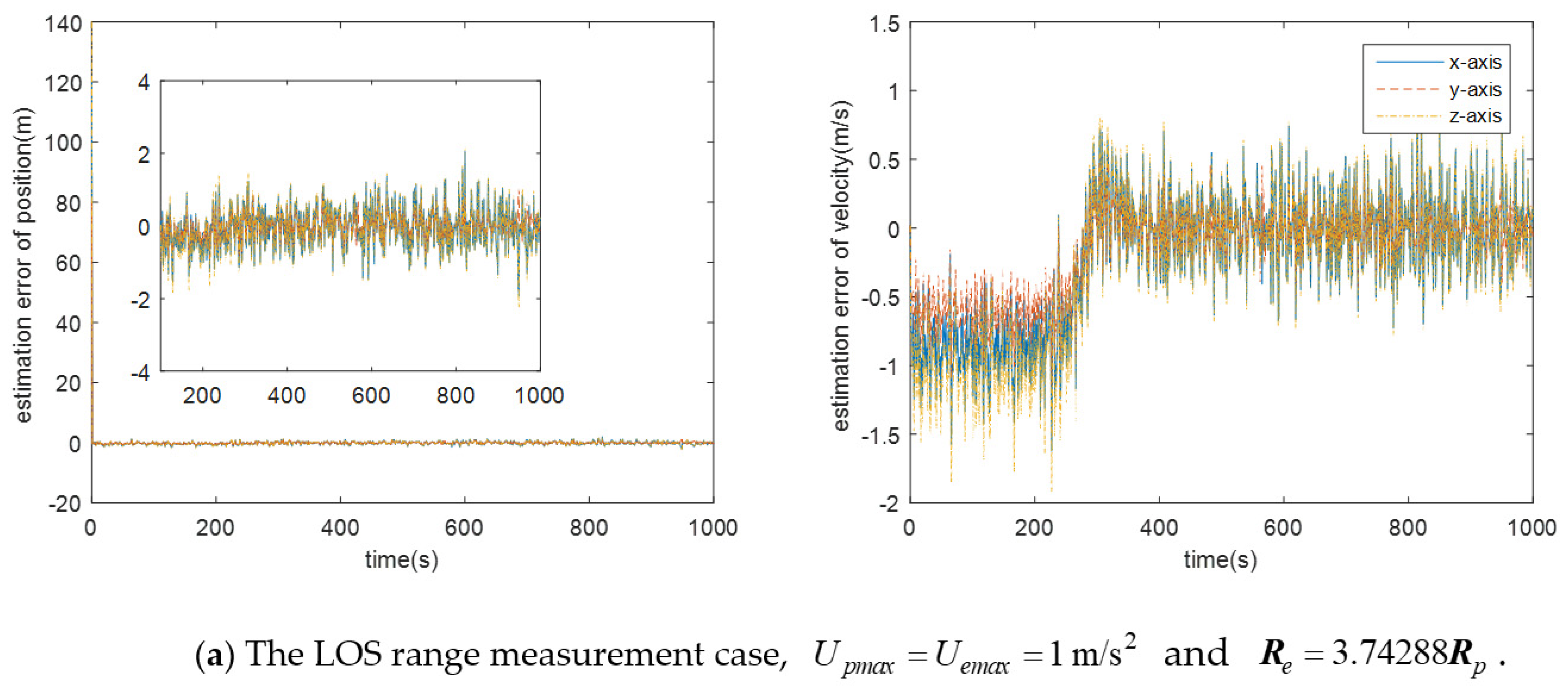
7.2. LOS Range Measurement Case

When angle and distance measurements are used for observation, the equivalent position measurement can be obtained through numerical calculation. The mean value and standard deviation of the measurement error are shown in Figure 6. Figure 6 also shows the Pursuer’s measurement precision for a 1 km range using the accuracy from Table 3. The equivalent position measurement error is 1.2 m (maximum).

In this paper, we only discuss the case with a limited maneuvering capabilities of the Pursuer and Evader because of the maximum thrust limit. First, the Pursuer and Evader use the same maneuver limit, as $U_{pmax}=U_{emax}=1{\mathrm{m}/\mathrm{s}}^2$. The Pursuer maneuvering weight matrix is $R_p=I_{3\times 3}\times {10}^5$ , while the Evader uses different maneuvering weight matrices, i.e., $R_e=2R_p, 2.5R_p, 3.74287R_p, 3.74288R_p,5R_p\mathrm{or}\infty R_p$, as shown in Figure 7.

$R_e=3.74288R_p$ is the boundary beyond which the Pursuer can approach the Evader when the LOS range measurement is used. Figure 8 shows the case where $U_{emax}=0.8{ \mathrm{m}/\mathrm{s}}^2$, and the Evader takes different maneuvering weight matrices $R_e=1.6R_p,2R_p\mathrm{or}2.5R_p$, respectively.

When the maneuver limit between the Pursuer and Evader is different, the Pursuer can gradually get close to the Evader if the limit of the Evader is smaller than the Pursuer, e.g., $R_e=1.6R_p$. The control strategy of the Evader is not considered when designing the control of the Pursuer, so the Pursuer cannot catch the Evader when $R_e=1.6R_p$. Therefore, the Pursuer can no longer get close to the Evader when the maneuvering amplitude of the Pursuer is lower than the limit, so a relatively stable distance between the Pursuer and the Evader exists in the game process.

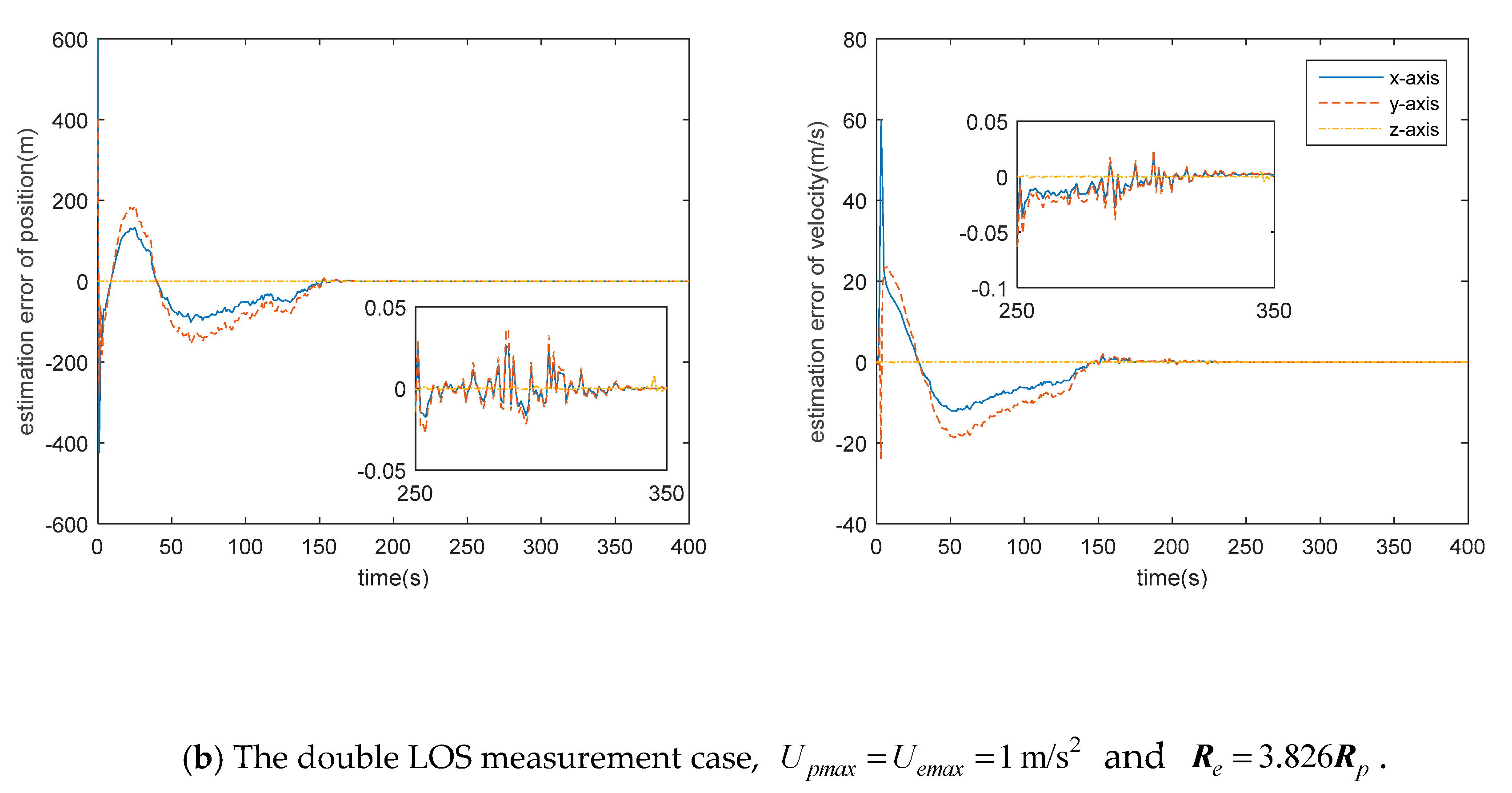
7.3. Double LOS Measurement Case

Similar to the discussion in the previous section. First, the Pursuer and Evader use the same maneuver limit, i.e., $U_{pmax}=U_{emax}=1{\mathrm{m}/\mathrm{s}}^2$. The Pursuer maneuvering weight matrix is $R_p=I_{3\times 3}\times {10}^5$ , while the Evader uses different maneuvering weight matrices, i.e., $R_e=2R_p,2.5R_p,3.825R_p,3.826R_p,5R_p\mathrm{or}\infty R_p$, as shown in Figure 9.

$R_e=3.826R_p$ is the boundary beyond which the Pursuer can approach the Evader when the double LOS measurement is used. Figure 10 shows the case where the Pursuer and Evader use different maneuver weights, i.e., $U_{pmax}=1{\mathrm{m}/\mathrm{s}}^2$, $U_{emax}=0.8{\mathrm{m}/\mathrm{s}}^2$.

Similar to the previous section, the Pursuer cannot catch the Evader when $R_e$ is small, because the control strategy of the Evader is not considered when designing the control of the Pursuer, such as $R_e=1.6R_p\mathrm{and}2R_p$. However, when $R_e$ is big enough, i.e., $R_e=2.5R_p$, the Pursuer can catch the Evader.

8. Conclusions

To solve the incomplete information game problem with a space non-cooperative target, this paper studied the optimal control algorithm based on the differential game theory where the unknown maneuver of the Evader is processed as colored noise. EKF was used to obtain the Evader’s relative state, and thus, observability analysis with different measurement methods is performed and its influence on the proposed algorithm is also shown in the fourth section. Numerical simulations were conducted to verify the proposed algorithm using different measurement models. The following conclusions are obtained:

(1)

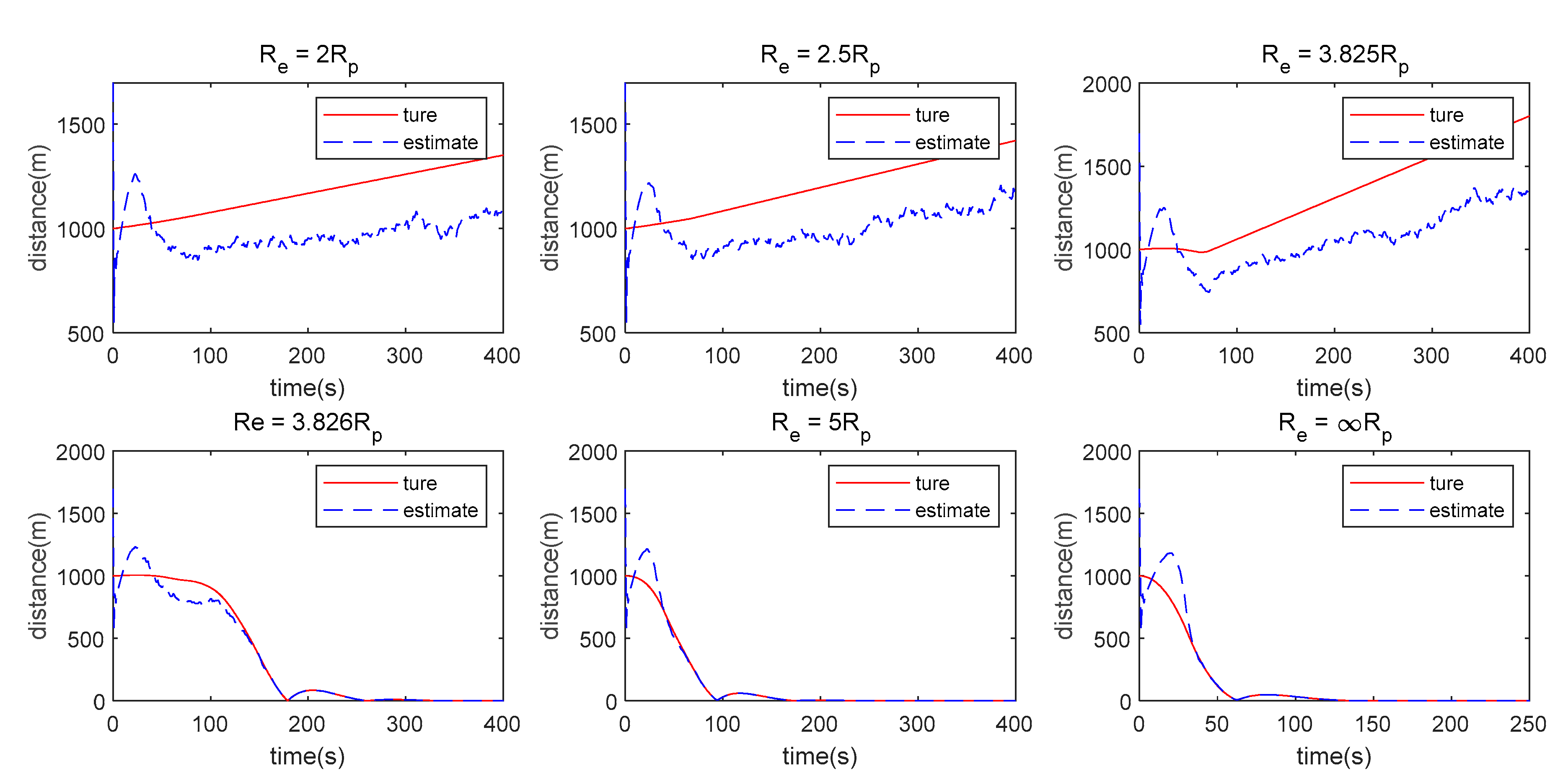
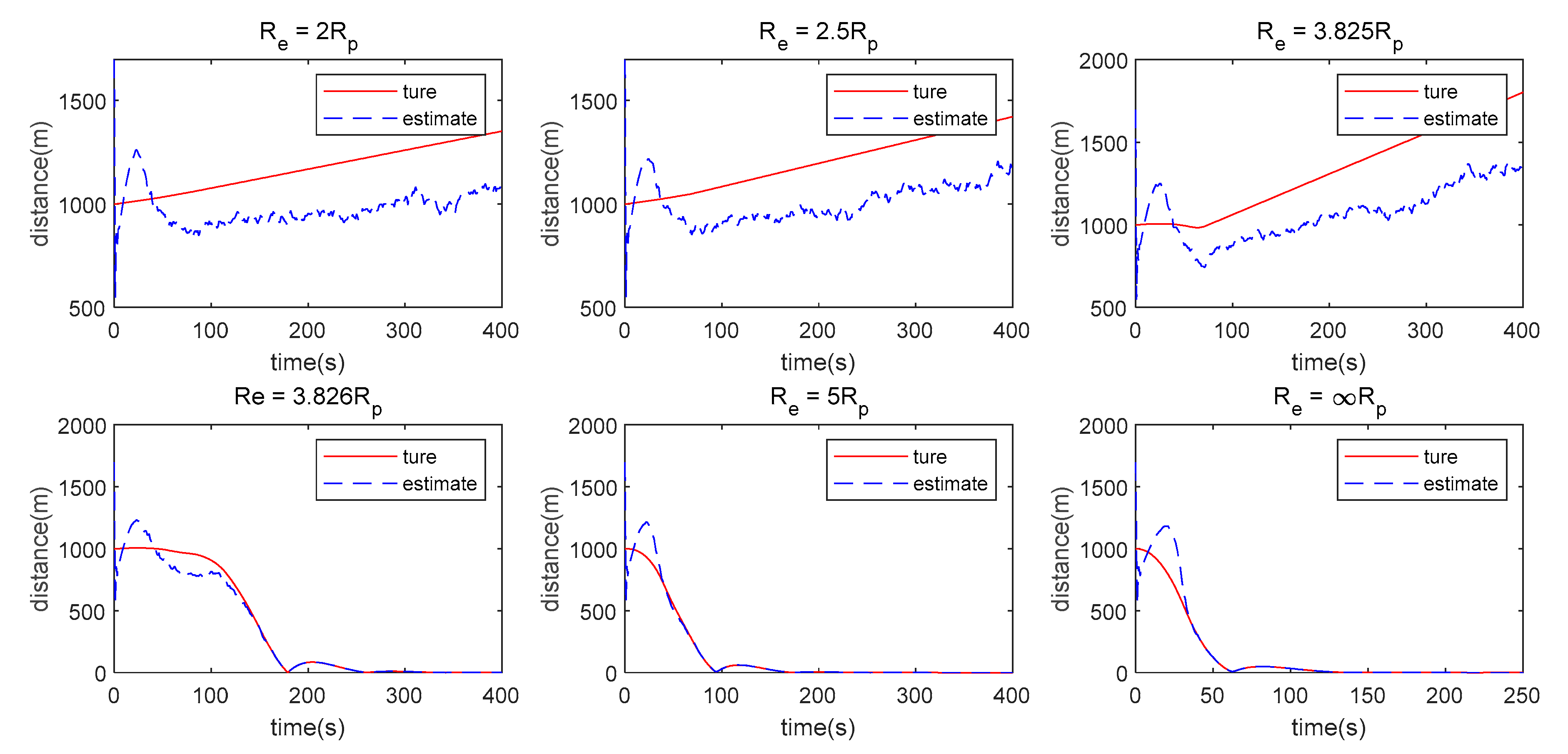
The measurement method has a great influence on the algorithm proposed in this paper. When single angle measurement is used, the Pursuer can approach the Evader using observation information at the beginning, but the chasing process cannot be maintained because of weak observability. However, the Pursuer can approach the Evader when LOS range or double LOS sensor measurements are used by the Pursuer.

(2)

There is still some position/displacement/distance estimation error, although observability is improved by adding the distance measurement or when the double LOS sensor measurement is used, as shown in Figure 11. Thus, the Pursuer cannot catch the Evader when $R_p \text{<}{R}_e<3.74288R_p$ in the LOS range measurement case, or $R_p \text{<}{R}_e<3.826R_p$ in the double LOS measurement case. The critical value of $R_e$ with which the Pursuer can catch the Evader will be smaller if $U_{emax}<U_{pmax}$.

(3)

The essence of the method proposed in this paper is that the Pursuer seeks the optimal control approaching the Evader under the assumption that the Evader’s maneuverability is lower than that of the Pursuer.

References

1. Geng, Y.Z.; Li, C.J.; Guo, Y.N.; James Douglas BIGGS. Rendezvous and docking of spacecraft with single thruster: Path planning and tracking control. Acta Aeronaut. Et Astronaut. Sin. 2020, 41, 323880. (In Chinese) [Google Scholar] [CrossRef]
2. Xu, Z.Y.; Chen, Y.K.; Qi, N.M.; Yang, Y. Active disturbance rejection control for spacecraft rendezvous and docking simulation system during proximity operations. Acta Aeronaut. Et Astronaut. Sin. 2016, 37, 1552–1562. (In Chinese) [Google Scholar] [CrossRef]
3. Sun, B.W.; Wang, D.Y.; Wang, J.Q.; Zhou, H.Y.; Ge, D.M.; Dong, T.S. Filter method for dimension reduction in spacecraft autonomous navigation based on sequence image. Acta Aeronaut. Et Astronaut. Sin. 2021, 42, 524971. (In Chinese) [Google Scholar] [CrossRef]
4. Gong, B.; Li, S.; Zheng, L.; Zhou, W. Angles-only relative navigation algorithm for close-in proximity of space non-cooperative target. J. Chin. Inert. Technol. 2018, 26, 173–179. [Google Scholar] [CrossRef]
5. Cohen, G.; Afshar, S.; Morreale, B.; Bessell, T.; Wabnitz, A.; Rutten, M.; van Schaik, A. Event-based Sensing for Space Situational Awareness. J. Astronaut. Sci. 2019, 66, 125–141. [Google Scholar] [CrossRef]
6. Delande, E.; Frueh, C.; Franco, J.; Houssineau, J.; Clark, D. Novel Multi-Object Filtering Approach for Space Situational Awareness. J. Guid. Control Dyn. 2018, 41, 59–73. [Google Scholar] [CrossRef] [Green Version]
7. Adurthi, N.; Singla, P.; Majji, M. Mutual Information Based Sensor Tasking with Applications to Space Situational Awareness. J. Guid. Control Dyn. 2020, 43, 767–789. [Google Scholar] [CrossRef]
8. Chen, Y.; Tian, G.; Guo, J.; Huang, J. Task Planning for Multiple-Satellite Space-Situational Awareness Systems. Aerospace 2021, 8, 73. [Google Scholar] [CrossRef]
9. Li, W.-J.; Cheng, D.-Y.; Liu, X.-G.; Wang, Y.-B.; Shi, W.-H.; Tang, Z.-X.; Gao, F.; Zeng, F.M.; Chai, H.; Luo, W.-B.; et al. On-orbit service (OOS) of spacecraft: A review of engineering developments. Prog. Aerosp. Sci. 2019, 108, 32–120. [Google Scholar] [CrossRef]
10. Sabatini, M.; Volpe, R.; Palmerini, G.B. Centralized visual based navigation and control of a swarm of satellites for on-orbit servicing. Acta Astronaut. 2020, 171, 323–334. [Google Scholar] [CrossRef]
11. Daneshjou, K.; Mohammadi-Dehabadi, A.A.; Bakhtiari, M. Mission planning for on-orbit servicing through multiple servicing satellites: A new approach. Adv. Space Res. 2017, 60, 1148–1162. [Google Scholar] [CrossRef]
12. Rousso, P.; Samsam, S.; Chhabra, R. A Mission Architecture for On-Orbit Servicing Industrialization. In Proceedings of the 2021 IEEE Aerospace Conference (50100), Big Sky, MT, USA, 6–13 March 2021; pp. 1–14. [Google Scholar] [CrossRef]
13. Isaacs, R. Differential Games; John Wiley & Sons: New York, NY, USA, 1965. [Google Scholar]
14. Friedman, A. Differential Games; American Mathematical Society: Providence, RI, USA, 1974. [Google Scholar]
15. Starr, A.W.; Ho, Y.C. Nonzero-sum differential games. J. Optim. Theor. Appl. 1969, 3, 184–206. [Google Scholar] [CrossRef]
16. Roxin, E.; Tsokos, C.P. On the definition of a stochastic differential game. Math. Syst. Theor. 1970, 4, 60–64. [Google Scholar] [CrossRef]
17. Nichols, W.G. Stochastic Differential Games and Control Theory. Dissertation for Doctoral Degree; Virginia Polytechnic Institute and State University: Blacksburg, VA, USA, 1971. [Google Scholar]
18. Ciletti, M.D. Results in the theory of linear differential games with an information time lag. J. Optim. Theor. Appl. 1970, 5, 347–362. [Google Scholar] [CrossRef]
19. Ciletti, M.D. New results in the theory of differential games with information time lag. J. Optim. Theor. Appl. 1971, 8, 287–315. [Google Scholar] [CrossRef]
20. Ciletti, M.D. Differential games with information time lag: Norm-invariant systems. J. Optim. Theor. Appl. 1972, 9, 293–301. [Google Scholar] [CrossRef]
21. Mori, K.; Shimemura, E. Linear differential games with delayed and noisy information. J. Optim. Theor. Appl. 1974, 13, 275–289. [Google Scholar] [CrossRef]
22. Wang, J. A Stackelberg differential game for defence and economy. Optim. Lett. 2018, 12, 375–386. [Google Scholar] [CrossRef]
23. Aumann, R.J.; Maschler, M.B. Repeated Games with Incomplete Information; MIT Press: Cambridge, UK, 1995. [Google Scholar] [CrossRef] [Green Version]
24. Harsanyi, J.C. Games with Incomplete Information Played by “Bayesian” Players, I–III Part I. The Basic Model. Manag. Sci. 1967, 14, 159–182. [Google Scholar] [CrossRef]
25. Kreps, D.; Wilson, R. Reputation and imperfect information. J. Econ. Theory 1982, 27, 253–279. [Google Scholar] [CrossRef] [Green Version]
26. Woodbury, T.D.; Hurtado, J.E. Adaptive play via estimation in uncertain nonzero-sum orbital pursuit evasion games. In Proceedings of the AIAA SPACE and Astronautics Forum and Exposition, Orlando, FL, USA, 12–14 September 2017; p. 5247. [Google Scholar] [CrossRef]
27. Woodbury, T.D.; Hurtado, J.E. Cooperative estimation in pursuit evasion games with bearing-only measurements. In Proceedings of the2018 AIAA Information Systems-AIAA Infotech@ Aerospace, Kissimmee, FL, USA, 8–12 January 2018; p. 0713. [Google Scholar] [CrossRef]
28. Aures-Cavalieri, K.D. Incomplete Information Pursuit-Evasion Games with Applications to Spacecraft Rendezvous and Missile Defense. Ph.D. Thesis, Texas A&M University, College Station, TX, USA, 2014. [Google Scholar]
29. Cavalieri, K.A.; Satak, N.; Hurtado, J.E. Incomplete information pursuit-evasion games with uncertain relative dynamics. In Proceedings of the AIAA Guidance, Navigation, and Control Conference, National Harbor, MD, USA, 13–17 January 2014; p. 0971. [Google Scholar] [CrossRef]
30. Woodbury, T.D. Estimation-Based Solutions to Incomplete Information Pursuit-Evasion Games. Ph.D. Thesis, Texas A&M University, College Station, TX, USA, 2019. [Google Scholar]
31. Liu, B.Y.; Ye, X.B.; Gao, Y.; Wang, X.; Ni, L. Strategy solition of non-cooperative target pursuit-evasion game based on branching deep rein-forcement learning. Acta Aeronaut. Et Astronaut. Sin. 2020, 41, 324040. (In Chinese) [Google Scholar] [CrossRef]
32. Linville, D.; Hess, J. Linear Regression Models Applied to Spacecraft Imperfect Information Pursuit-Evasion Differential Games. In Proceedings of the AIAA Scitech 2020 Forum, Orlando, FL, USA, 6–10 January 2020; p. 0952. [Google Scholar] [CrossRef]
33. Ye, D.; Tang, X.; Sun, Z.; Wang, C. Multiple model adaptive intercept strategy of spacecraft for an incomplete-information game. Acta Astronaut. 2021, 180, 340–349. [Google Scholar] [CrossRef]
34. Li, Z.Y.; Zhu, H.; Luo, Y.Z. An escape strategy in orbital pursuit-evasion games with incomplete information. Sci. China Technol. Sci. 2021, 64, 559–570. [Google Scholar] [CrossRef]
35. Oshman, Y.; Davidson, P. Optimization of observer trajectories for bearings-only target localization. IEEE Trans. Aerosp. Electron. Syst. 1999, 35, 892–902. [Google Scholar] [CrossRef]
36. Battistini, S.; Shima, T. Differential games missile guidance with bearings-only measurements. IEEE Trans. Aerosp. Electron. Syst. 2014, 50, 2906–2915. [Google Scholar] [CrossRef]
37. Fonod, R.; Shima, T. Estimation enhancement by cooperatively imposing relative intercept angles. J. Guid. Control Dyn. 2017, 40, 1711–1725. [Google Scholar] [CrossRef]
38. Battistini, S. A Stochastic Characterization of the Capture Zone in Pursuit-Evasion Games. Games 2020, 11, 54. [Google Scholar] [CrossRef]
39. Curtis, H. Orbital Mechanics for Engineering Students; Elsevier Ltd.: Amsterdam, The Netherlands, 2013. [Google Scholar]
40. Grzymisch, J.; Fichter, W. Observability criteria and unobservable maneuvers for in-orbit bearings-only navigation. J. Guid. Control Dyn. 2014, 37, 1250–1259. [Google Scholar] [CrossRef]
41. Jagat, A. Spacecraft Relative Motion Applications to Pursuit-Evasion Games and Control Using Angles-Only Navigation. Ph.D. Thesis, Auburn University, Auburn, AL, USA, 2015. [Google Scholar]
42. Nash, J.F. Equilibrium points in n-person games. Proc. Natl. Acad. Sci. USA 1950, 36, 48–49. [Google Scholar] [CrossRef] [Green Version]
43. Pontryagin, L.S.; Botyanskii, V.G.; Gamkrelidze, R.V.; Mishkenko, E.E. The theory of optimal processes I. The maximum principle. Izvest. Akad. Nauk SSSR Ser. Mat. 1960, 24, 3–42. [Google Scholar]
Figure 1. Illustration of the virtual Chief orbital coordinate system.
Aerospace 08 00211 g001
Figure 2. Pursuit-Evasion Games in the virtual Chief orbital coordinate system.
Aerospace 08 00211 g002
Figure 3. Illustration of the observation model when a double LOS sensor measurement is used by the Pursuer.
Aerospace 08 00211 g003
Figure 4. The entire architecture of the method proposed in this paper.
Aerospace 08 00211 g004
Figure 5. Distance between the Evader and Pursuer when the Pursuer uses a single LOS measurement and the Evader uses different maneuver weights.
Aerospace 08 00211 g005
Figure 6. The mean value and standard deviation of the Evader’s position measurement error with LOS range measurement when the distance between the Pursuer and the Evader is 1 km.
Aerospace 08 00211 g006
Figure 7. Distance between the Evader and Pursuer when the Evader and Pursuer use the same maneuver limit while the Evader uses different maneuver weights.
Aerospace 08 00211 g007
Figure 8. Distance between the Evader and Pursuer and maneuver of the Evader and Pursuer when the Evader and Pursuer use different maneuver limits while the Evader uses different maneuver weights.
Aerospace 08 00211 g008
Figure 9. Distance between the Evader and Pursuer when the Evader and Pursuer use the same maneuver limit while the Evader uses different maneuver weights.
Aerospace 08 00211 g009
Figure 10. Distance between the Evader and Pursuer and the acceleration in the double LOS measurement case where u e 0 .
Aerospace 08 00211 g010
Figure 11. Estimation error of the Evader’s relative state in different cases.
Aerospace 08 00211 g011aAerospace 08 00211 g011b