1. Introduction
Aircraft manufacturers and operators face an ever-increasing economic pressure while dealing in a highly complex and competitive environment. Typically characterized by low profits and high investment cost [
1], strategic decisions for or against a product or strategy can impact the company for decades to come [
2], especially if the long operational phase of aircraft are considered. Thus, a priori analyses of the expected economic impact of any major decision are of eminent importance in profit driven businesses [
3]. These Overall Economic Assessments (OEAs) are often integrative in nature, i.e., information from various stakeholders and disciplines such as operations, maintenance, aircraft performance, as well as relevant boundary conditions and off-design cases have to be collected and combined. Their output is expressed in a set of differential metrics (e.g.,
cost) which represent the expected superiority of one alternative over another. In aeronautical practice, these OEAs are mostly based on Cost Estimation Relationships (CERs), which correlate selected aircraft characteristics or operational parameters with the certain cost elements provided in confidential economics databases from the manufacturer or operator [
4,
5].
Although CERs are quick to implement and fast to evaluate, their applicability is limited in terms of what can be assessed. Strictly speaking, the results are valid only for the operation of former and current aircraft generations, and deviations from them often do not extrapolate well [
4,
6,
7]. Furthermore, the fixed nature of static equations requires that the Object of Interest (OoI) directly affects the input parameters, or else the impact remains unnoticed. Another notable shortcoming, especially when operational aspects are of interest, is the limited consideration of the complex interrelations of the air transportation system. These cover the temporal, spatial, and partially the physical domain. For instance, the effect of specific maintenance actions (of both scheduled and unscheduled nature) on the aircraft’s performance and airline’s economics cannot be accounted for with the existing conventional methods. Although there are specific studies and methods that deal with such detailed problems on their own, their consideration in a comprehensive OEA is rarely seen. Finally, the lack of a standard assessment framework impedes the comparability of technologies in terms of their overall economic and operational impact.
Therefore, a framework is needed which tackles these shortcomings. For one, this tool should enable the analysis of various products, regardless of whether it is an aircraft design, a physical technology, an operational decision or a maintenance strategy. For study cases where information is rare, the tool should provide default assumptions, which should be easily replaceable when more detailed information and/or models become available. Considering the long operational times of aircraft, another central objective is the ability to capture not only primary (i.e., “intuitive” or “obvious”) effects of an OoI induced change in the aircraft’s life but also secondary ones occurring much later (i.e., “down the river”).
To this end, an object oriented, modular and hierarchical detail oriented framework for OEA is developed which incorporates a discrete event simulation of an aircraft’s life cycle. These events include, but are not limited to, the order and delivery of aircraft, various flights, scheduled and unscheduled maintenance, periodically recurring payments, and the resale of the aircraft. This tool is customizable by design, where nearly all parts of the code can be replaced and tailored for the problem at hand, while the source code itself remains untouched. The present paper introduces this framework (which is intended to be publicly available in the future), the methodology behind it, and demonstrates its capabilities with a case study. For the latter, the on-wing maintenance action of engine cleaning is modeled and assessed in terms of fuel burn and overall economic efficacy on an Airbus A321 aircraft. This study includes a (simplified) model of the engine degradation (i.e., a gradual increase of Exhaust Gas Temperature (EGT)) and the repercussions on the specific fuel consumption and Engine Shop Visits (ESVs). By considering the interrelations between the predicted deterioration, the resulting fuel efficiency and the current fuel price, the cost for an engine wash event and the time until the next shop visit, a decision making algorithm of the technology aiming for the lowest operating cost is studied.
The remainder of this paper is structured as follows.
Section 2 provides some fundamentals on economic assessments in general and aeronautical engineering. Additionally, relevant literature and tools that are comparable to the present work are discussed.
Section 3 presents the newly developed framework starting with central goals and requirements. Subsequently, the modular program architecture is presented, which is followed by a description of the default modules and methods. In
Section 4, the aforementioned exemplary technology assessment is performed. This includes a description of the inputs, the customized module for optimized engine wash event scheduling, and its impact on the airline’s economic value. The paper concludes with a summary in
Section 5.
2. Fundamentals
Although the topic of cost estimation has been intensively studied in engineering sciences in the past [
8,
9], there is no consistent standard or even taxonomy apparent [
10]. Ambiguities can be found in (a) the nature of the methods used, which influences the effort for and accuracy of the study; (b) the temporal space that is covered by the analysis, i.e., one, multiple, or all life cycle phases; and (c) the extent of the considered monetary elements. This section attempts to provide an overview in these domains with the goal of situating the scope of the presented framework adequately.
2.1. General Cost Estimation Methods
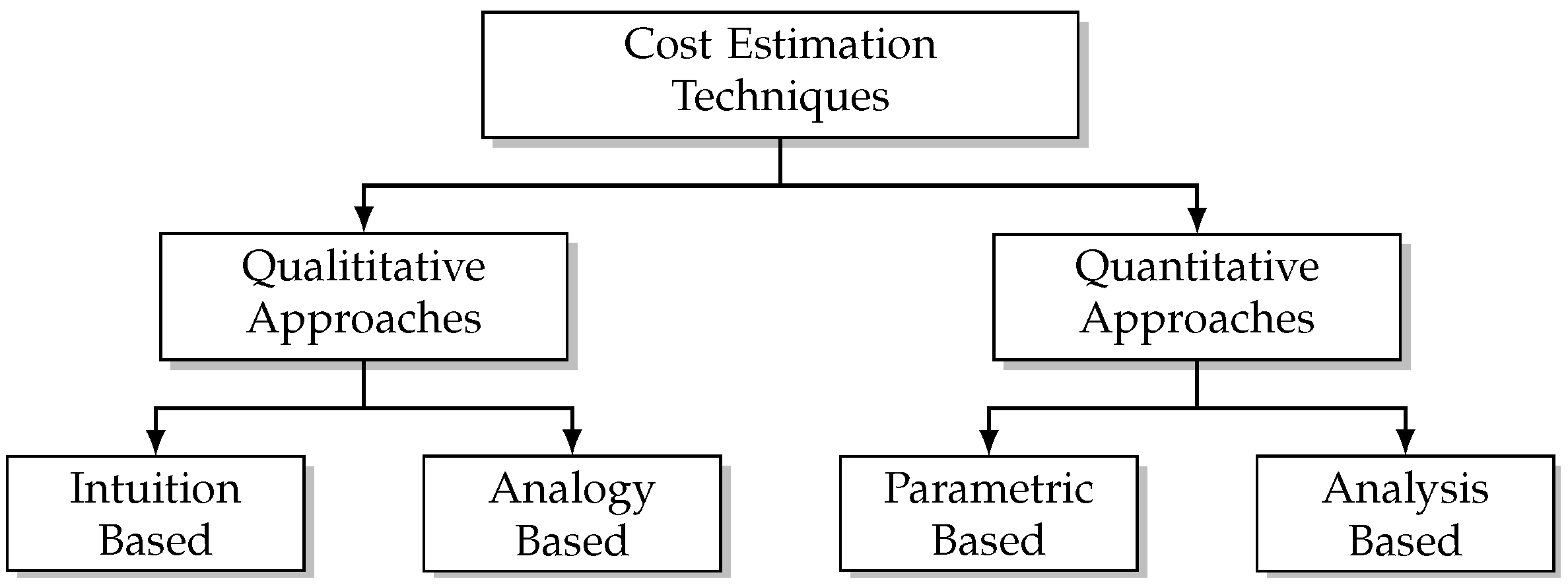
Various classifications for cost estimation methods exist, including top-down and bottom-up, genetic and causal, as well as qualitative and quantitative approaches. As Altavilla et al. [
2] showed, the latter breakdown is most prominent in the general engineering design domain, see
Figure 1. Each approach has its own benefits, drawbacks and ideal phases of applicability. The methods in the qualitative category require only little information but are less accurate and hence more useful in earlier design phases. As they heavily depend on historic data and expert knowledge, particular care has to be taken with respect to their applicability. Quantitative techniques also make use of historic data but incorporate an elevated level of modeling. This ranges from a combination of product specific and regression based CERs up to detailed event and/or agent based modeling. As such, the level of information required to perform such an estimation is comparatively high, making them more appropriate in later design phases.
Due to the complexity of setting up a cost evaluation process, companies and research institutions often confine themselves to one or few particular techniques, which are usually integrated in (partially) automated product design frameworks. However, when it comes to assessments in multidisciplinary and complex environments such as the air transportation system, a modular, flexible, extensible, and method overarching system is necessary, as correctly described in Leung [
12] and Curran et al. [
4]. As it will be explained in
Section 3, the work presented here aims to fill this gap by combining multiple techniques, which allows to cover development stages ranging from early to detailed design without the necessity to change the basic procedure or underlying assumptions.
2.2. Valuation Practice in Aeronautics
While the previously mentioned techniques are more universal in nature, the classification in this subsection is more specific to the aeronautical engineering domain. In here, available methods mainly differ in considered temporal phases and modeled cost elements. They can be clustered into Direct Operating Cost (DOC) methods and life cycle based approaches. Both are described below.
2.2.1. Direct Operating Cost Methods
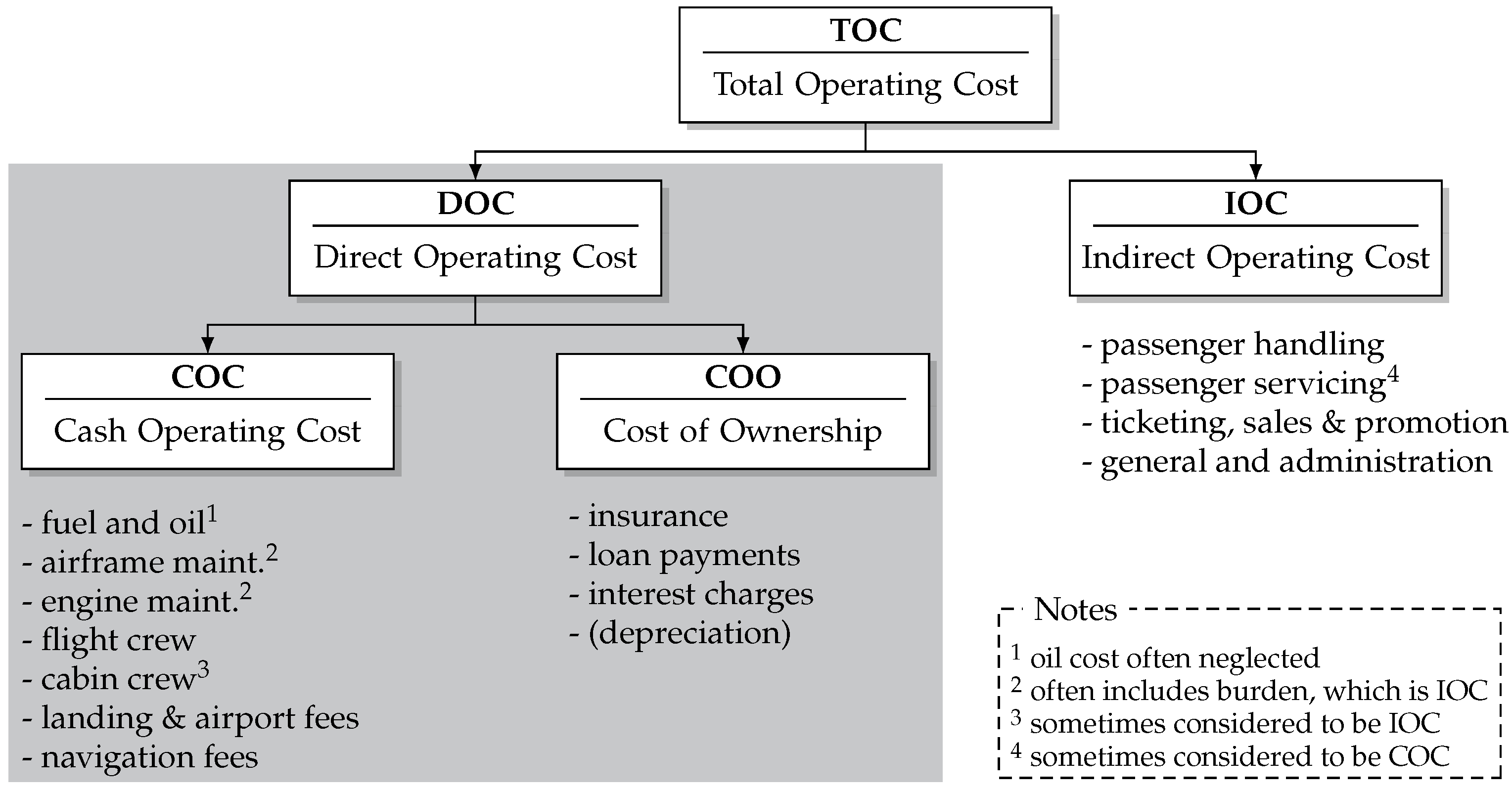
DOC represent cost elements that are directly affected by the aircraft such as fuel, maintenance, various fees, and aircraft financing expenses and, together with the Indirect Operating Cost (IOC), make up the Total Operating Cost (TOC) of an airline, as shown in
Figure 2. As it is common to compare different aircraft using their associated DOC per year, per flight hour, or per flight cycle [
13], parametric techniques were developed to predict these cost based on easily available aircraft information [
14,
15]. These techniques are known as DOC methods and are a prevalent approach for the evaluation of aircraft designs, technologies, and occasionally operational procedures [
4].
A variety of DOC methods is available throughout research and industry. The most frequently used ones are the NASA method [
16], the Association of European Airlines (AEA) methods [
17,
18], and one presumably originating from Lufthansa [
19], which was last updated in 2010 [
20]. Applications include technology unspecific studies such as in Lee et al. [
21] or Ali and Al-Shamma [
22], where various conventional aircraft are assessed economically and compared to one another, as well as more specific investigations such as in Xu et al. [
23], Elham and van Tooren [
24], and Pohya et al. [
25] where formation flights, winglet shapes, and hybrid laminar flow control are evaluated, respectively. An example of a debatable application can be found in Cuerno-Rejado et al. [
26], where a highly unconventional joined-wing aircraft design was compared to a conventional reference using the DOC approach. The result showed no changes in maintenance or ownership expenses (the latter was omitted in the study, while its impact was mentioned qualitatively), but only in fuel cost, which is questionable considering the substantially different airframes. A more recent stream recognizes the limitations of available methods to accurately predict maintenance cost and hence create their own CERs using more specific input parameters for the (static) equations, e.g., Fioriti et al. [
27].
As a parametric technique, DOC methods suffer from typical CER limitations. For instance, the operational and financial data of airlines, on which the methods are based on, are typically not available to the public. This makes it difficult to decide whether an OoI is inside or outside of the area of applicability. Additionally, it is not possible to quantify the accuracy or associated uncertainty when using these CERs. Due to their top-down regression approach, relevant repercussions of one event (e.g., an unscheduled maintenance that is required) on another (e.g., the next flight(s)) cannot be captured.
Table 1 summarizes the characteristics of DOC methods.
2.2.2. Life Cycle Based Methods
With the increased computational power and integrative approach to product design, a shift towards a more holistic and life cycle driven approach has been observable [
28,
29]. In the aviation sector, these typically take one of two forms:
- (a)
Those that focus on the long operational phase of aircraft, where temporal effects such as learning curves and aging are investigated and the complexity of the air transportation system is modeled with more detail (e.g., Justin and Mavris [
30]).
- (b)
Those following the “cradle to grave” approach incorporating all life cycle phases. This is usually comprised of the manufacturing, operational, and end of life phase and follows the integrated product development paradigm (e.g., Curran et al. [
31]).
To differentiate these two streams, the former is called
life cycle costing (LCC), while the latter is termed
whole life cycle costing, (WLCC) which is adapted from the nomenclature in civil engineering (e.g., in Abdelhalim Boussabaine [
29] and Viavinette and Faulkner [
32]) as well as general cost engineering (e.g., Altavilla et al. [
2]).
Compared to the DOC methods, the added value of the LCC approach is created by the consideration of learning curves, aging and degradation effects, or other case specific aspects (e.g., modifications or retrofits during a major maintenance check and the assessment on fleet level, as investigated in Pohya et al. [
33]). LCC methods can give valuable insights on how the (economic) efficiency of a product changes over time (e.g., through deterioration) and what countermeasures (e.g., through maintenance) are efficient. However, due to their detailed nature, they are often specifically tailored to the case study at hand. This typically requires a tedious collection of detailed information which is hardly reusable. Moreover, such specific approaches do not ensure comparability of different studies to one another. Generic LCC models are rare and seldom publicly available.
The WLCC approach typically expands the classical manufacturers’ perspective on product design by the operators’ point of view, i.e., by direct operating cost. The aim is to develop a product that is not only cost efficient in production but is also competitive in operation. Similar to DOC methods, WLCC methods make use of CERs and calculate Research, Development, Testing, and Evaluation (RDTE) cost as well as recurring and non-recurring cost using aircraft attributes (e.g., aircraft weight) and manufacturing parameters (e.g., cadences). As such, they suffer from similar drawbacks as DOC methods, e.g., they neglect long-term effects and process induced repercussions and do not allow flexibility and extensibility outside of the static input parameter space. Examples of well established WLCC methods can be found in Raymer [
34] and Roskam [
35]. The following summarizes the prevalent valuation practice in aeronautics:
As a top-down tool, DOC methods are fast and easy to use but show a lack in their scope of applicability, both in temporal space and OoI [
4].
LCC methods tackle this limitation by considering age related effects and often a case specific modeling of the environment but require laborious preparation as a bottom-up approach. Due to the more tailored nature, their versatility and subsequently comparability is often limited.
WLCC methods are primarily used for integrated product development and expand the manufacturers’ point of view by operating cost. As they are often based on CERs, they suffer from the same detriments as DOC methods.
With the dominating CER approach taken by most studies, the impact of specific decisions (e.g., maintenance actions) on the complex air transportation system cannot be captured in detail.
Additionally, the nature of costing methods neglects revenues and hence reduces the economic value of a technology to its impact on the expenditures. Depending on the OoI, the loss of revenues due to a missed flight may have an even greater impact on the overall airline economics than the cost of correcting the cause.
2.3. Comparable Work
To situate the assessment environment presented in this study, comparable work is briefly reviewed here. This selection does not claim to be exhaustive but rather informative and intends to give an overview of current economic evaluation research in aerospace engineering.
Frank et al. [
36] present a modular and design oriented environment for assessing the flying, economic, and safety performance of suborbital vehicles. While modules such as the aerodynamics, structures, and propulsion leverage advanced physics and surrogate based approaches, the life cycle cost were estimated with CERs. A similar environment for spacecraft assessment is presented by Yao et al. [
37]. Here, the focus lies less on exploring the design space and more on the comparison of different systems during their operational phase and their impact on the Net Present Value (NPV). Furthermore, the authors made an effort to provide Uncertainty Quantification (UQ) features by integrating Monte Carlo Simulation (MCS) capabilities into the framework.
Thokala et al. [
38] focus on integrated aircraft design and estimate the acquisition cost using a hierarchical product definition tool called DecisionPro [
39], while using a discrete event simulation named Extent [
40] for estimating the operating and maintenance cost. Combined in a MATLAB environment, their framework is also capable of performing Design of Experiments (DOE) and MCS. This framework was used to design unmanned air vehicles in Thokala et al. [
41] and to calculate overall maintenance cost of aero-engines in Wong et al. [
42]. Both Extent and DecisionPro are well developed and commercially available. However, as such, their flexibility and capability to be custom-tailored to more complex OoIs is limited.
Zhao et al. [
43] recognize the need for an aircraft assessment method that is applicable both in early and detailed design. They suggest a two-leveled approach, where first, costs are estimated with preliminary weight based estimation relationships. Once detailed information in the form of a bill of material is available, WLCC can be calculated using more detail driven CERs, although again with weight as the single cost driving parameter. Thus, the available level of detail when modeling relevant interactions remains restricted. Xu et al. [
44] also take the aircraft designers perspective into account and briefly present an object-oriented WLCC tool which tracks the cost of manufacturing, operating, maintaining, and disposal of components. Although this framework seems to model the components in detail, it is not clear how the objects interact, costs are calculated, and whether the framework offers interfaces for customization.
Justin and Mavris [
30] developed a modular framework named ICARE, which takes the airline’s perspective and calculates all aircraft and engine related operating cost and revenues. These include ownership cost; base; heavy component (including the engines); and unscheduled maintenance cost, fly-away cost, and ticket and ancillary revenues. Similar to the framework presented in this paper, ICARE combines various literature and databases to calculate these elements and is able to quantify the value of different aircraft and engines. However, it seems as ICARE incorporates neither a Discrete Event Simulation (DES) nor agent-based modeling approach for capturing secondary impacts nor to have the inherited capability to be extended and customized to a particular OoI at hand.
To summarize, the majority of the discussed aeronautical assessment frameworks focus on aircraft design and the manufacturers’ perspective, strongly simplifying the interaction-intensive operational phase. Furthermore, the environments show a lack of ability to be customized to different case studies. Few acknowledge the fact that the level of information varies significantly throughout the product development and hence provide hybrid models with low and high level methods. The space sector pursues a more advanced and modular approach, while uncertainties in assumptions and scenarios are addressed with the provision of MCSs capabilities.
3. Evaluation Framework
The Python based framework named Life Cycle Cash Flow Environment (LYFE) aims to provide a generic (i.e., not project or case specific) environment. This section presents key goals and requirements (
Section 3.1), explains the program characteristics (
Section 3.2), and describes the default modules and methods (
Section 3.3). It should be noted that, due to the required flexibility of the framework, not all available methods and features can be discussed in one paper. Thus, the following is rather a representative excerpt of the functionalities.
3.1. Goals, Requirements, and Scope
The vision of LYFE can be described as:
LYFE is the standardized and universally accepted cost-benefit tool for aeronautical applications for researchers and industry alike.
To make this possible, a variety of different aspects have to be considered.
Table 2 summarizes LYFE’s top-level goals, requirements, and the scope delineation. In addition to these features, the two essential and unique characteristics of LYFE as a generic OEA framework are (a) the incorporation of a discrete event simulation and (b) its customizability through the modular program structure.
3.2. Program Characteristics
The goals, requirements and intended scope of LYFE lead to its specific program structure and characteristic features, which are described next.
3.2.1. Program Structure
LYFE itself acts as a top-level caller, which reads settings defining how the simulation will be run (e.g., single simulation, sensitivity analysis, MCS). Once these are processed, the core module AirLYFE takes over and performs an aircraft-centered and operator oriented simulation. This includes, but is not limited to, the purchase of the aircraft; performed flights; scheduled and unscheduled line and base maintenance with corresponding downtimes; monthly recurring costs of any kind, such as insurance, interest, or leasing rates; and the resale, recycling, or disposal of the aircraft. The level of detail varies with the users’ level of available information. If, for example, certain fees or maintenance cost are unknown, regression equations provide estimated values (similar to the approach of DOC methods). Alternatively, custom functions or lookup tables for the event attributes can be specified.
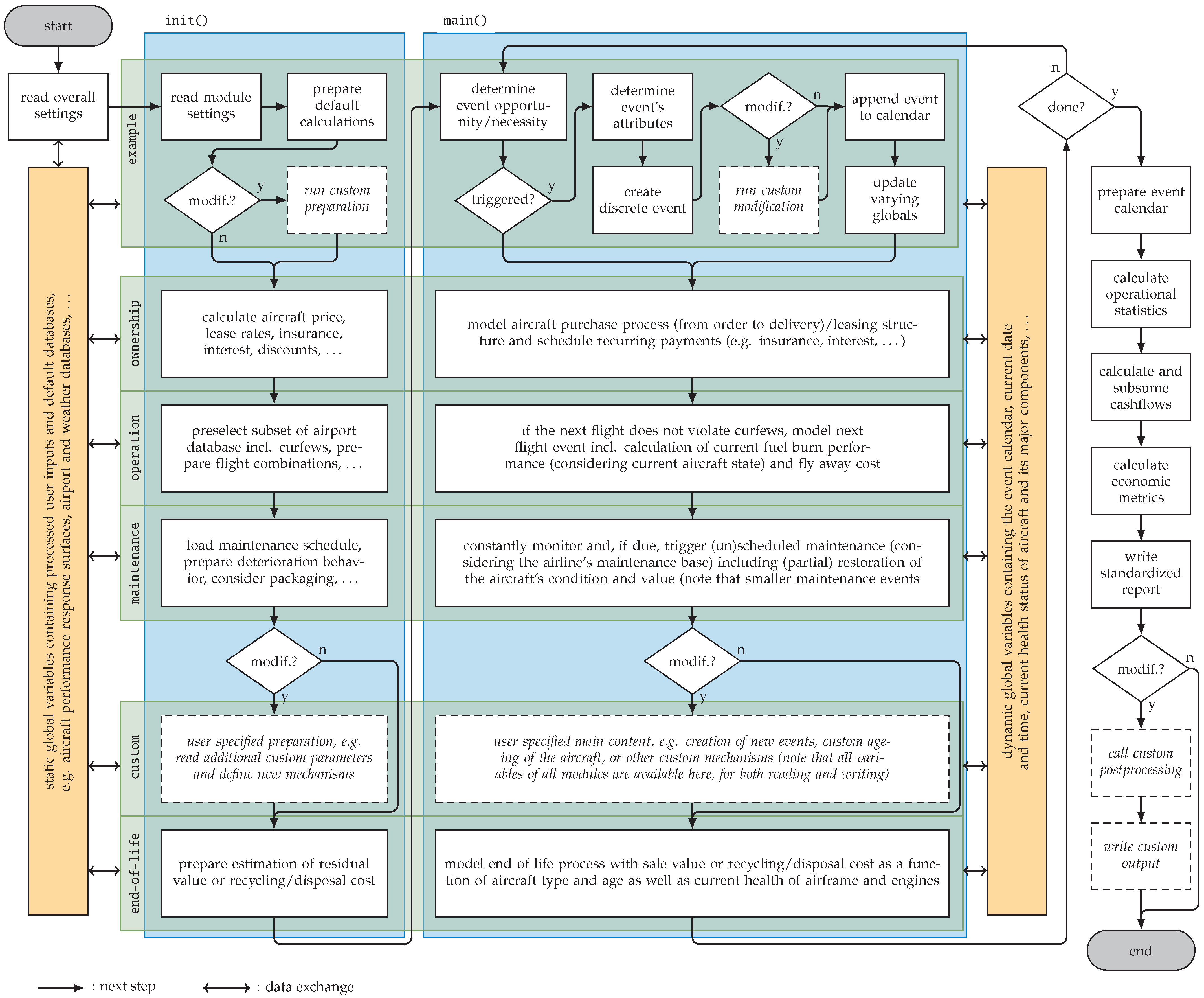
Figure 3 shows a schematic overview of the modular and customizable designed program structure.
The simulation starts with reading and processing the user inputs and making it available for each and every submodule. This also contains various databases, which will be explained later. Afterwards, the submodules are called. Each consists of an initialization and a main function, with a pseudo code given in Code Excerpt A1 in the
Appendix B. In the initialization part, preparatory work is performed, which aims to speed up the overall runtime. This includes precalculating rates, selecting relevant airports out of the database, and various other submodule specific tasks. After all submodules have been initialized, the simulation enters a while loop, calling the submodules’ main functions, which all have the same basic structure. At first, a set of
n constraints is used to determine whether one of the events that the submodule can create is due, i.e.,
Here, and describe the boolean and simulation parameter space, and , , , and represent the fixed and user specified, the fixed and module specific, the customization, and the dynamically changing domain, respectively. These constraints may, for instance, consider the aircraft’s health status for maintenance events, the operational schedule for flight events, or specific user written algorithms. If no event is due, the submodule is skipped and the simulation enters the next one. If an event is due, the respective event instance is created and filled with relevant attributes such as the duration, associated cost and revenues or, more specifically, the route which is flown or the interval trigger which caused the maintenance action. This event is then appended to an event calendar, which triggers an update of several simulation parameters. These include, for instance, the current simulation date and time or the condition of the aircraft and its components. Each submodule has access to two types of databases (in the sense of globally accessible sets of data and variables). The first is static in nature and holds parameters that do not change throughout the simulation, including aircraft performance maps, generic airport information, or user specified configuration files. The second is more dynamic and holds current snapshots of changing parameters, such as the event calendar itself, the current simulation time and date, and the asset’s (i.e., aircraft’s and/or engine’s) current condition. The simulation continues in the while loop until the OoI specified lifetime is over. This triggers the automatic report generation, which calculates not only operational efficiencies and statistics but also generic economic parameters. If desired, more specific metrics can be defined in the custom report generation. It should be noted that this process always runs at least twice: once for the reference case and once for the case under study. The overall results are then usually expressed as an absolute or relative change, e.g., NPV.
3.2.2. Discrete Event Simulation
The goal to capture both primary and secondary effects throughout the life cycle prescribes a DES combined with an object oriented approach. Primary effects are those that affect the OoI (or a stakeholder) immediately. Secondary effects are those that occur either much later or as a result of a more complex interaction network. For instance, a certain technology may affect the fuel burn and subsequently fuel cost (primary), whereas a maintenance action for said technology may lead to a prolongation of the downtime, affecting the subsequent flight schedule (secondary). Combined with the later explained customizability, the DES approach ensures that various decision making strategies can be implemented and evaluated with respect to their primary and secondary effects on the life cycle.
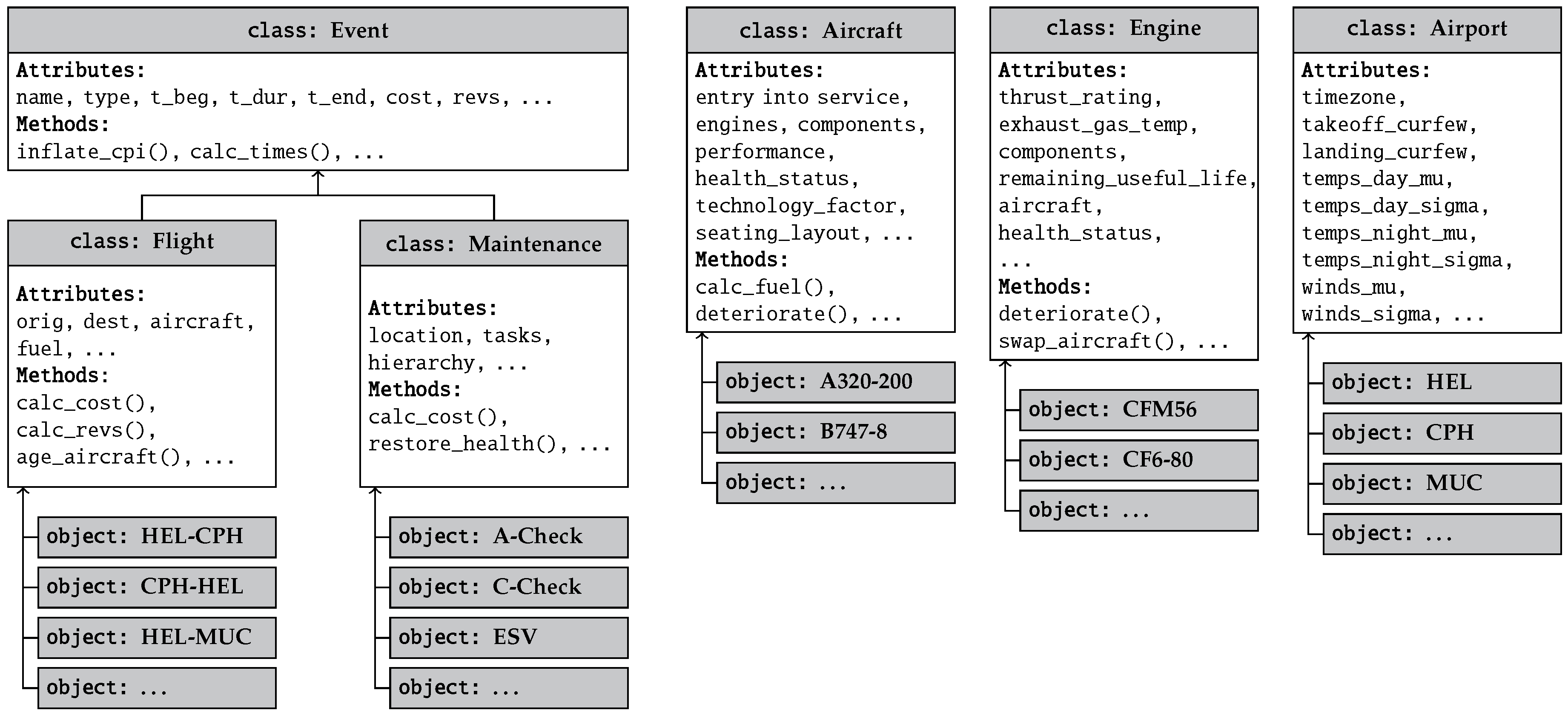
In LYFE, each event is an object with certain attributes, depending on the respective class definition. The event’s parent class definition includes the discrete beginning, duration, and finish time, as well as cost and revenue dictionaries. Child class definitions are specific to the type of event. Flight events for example include the information of the origin and destination airport, the aircraft that flies this route, associated fees, and many other elements. Apart from the event, the assets (i.e., aircraft and engines) and databases (e.g., airports) have their own classes, attributes and methods, see
Figure 4.
The event calendar grows dynamically with each appended event and, when the simulation is finished, contains anywhere between 50 and 300 k individual events per aircraft, depending on the use case and considered lifetime. The required runtime for a full simulation varies between 30 s and two minutes (on a regular single-core CPU laptop). An excerpt of a simulated event calendar is shown in
Figure 5, including flights from and to the aircraft base, a few maintenance checks, and some monthly recurring payments.
Each time an event is appended into the event calendar, the global clock is updated to the event’s end time, and two routines are triggered. The first includes a deterioration of the aircraft’s and engine’s health, e.g., through general aging or specified engine degradation. The second inflates the event’s associated cost and revenues to (a) the current simulation time, (b) a predefined fiscal year for the later calculation of economic metrics, and (c) the source’s fiscal year. The latter primarily serves verification and debugging purposes. It should be noted that, given the decades of an aircraft’s operational time, the correct consideration of the time value of money is crucial. Therefore, the fiscal inflation procedure itself uses the Consumper Price Index (CPI) published in [
45] for historic simulation times and a default of 2% annual inflation for future cash flows.
3.2.3. Modularity and Customizability
Apart from software engineering reasons and collaboration advantages, the key reason behind the modularity is that it enables customization on different levels. As it is highly difficult to code a framework that, by default, is able to model all relevant aspects of all potential case studies while not being prohibitive in runtime and complexity, the essential paradigm was to provide a high-quality standard set of methods and functions with the ability to be modified and extended through defined interfaces. There are several built-in ways of customization:
Choosing alternative default methods: The individual modules typically offer different methods for triggering events and calculating attributes. As it will be described in more detail in
Section 3.3, this includes whether the aircraft is purchased or leased, a flight schedule is flown sequentially or randomly, maintenance is performed on an interval and/or condition base, and whether the aircraft is sold or disposed of at its end of life. These features are well documented and require no coding effort, as all inputs are provided either through an Excel sheet or configuration text file.
Modify events that are about to be appended: When researchers wish to alter a default method to recalculate or calibrate an event’s attribute (e.g., cost, revenues, or fuel burn), they can
modify the event right before it will be appended to the calendar. If this option is set, AirLYFE calls the user written modifying function from within the simulation and expects a modified event in return, which is shown in the upper part of
Figure 3 (dashed boxes). An example would be an adjustment of fuel burn that considers airport (e.g., runway altitude) and weather specific parameters (e.g., wind speed and temperature). This customization represents the lowest level code intrusion, as the calling mechanisms remain untouched and no
new events are created, while the effort and required coding experience are low.
Add a custom module: If additional events are required, users may write their own
custom module and make it available through the predefined interfaces shown in the lower part of
Figure 3. In this case, AirLYFE runs the initialization as well as the main function of the custom module in the same way as with the other submodules. Since the static and dynamic global variables are also accessible, users have a higher degree of flexibility and can, for instance, trigger a particular maintenance action by setting the corresponding Remaining Useful Life (RUL) to zero. Examples for custom events include randomly occurring damages due to foreign objects, a specific flight event that is not foreseen in the standard schedule, or a specific maintenance event in which the aircraft undergoes a certain modification leading to a change in the upcoming maintenance schedule. This includes the execution of airworthiness directives, service bulletins, or engineering orders. Furthermore, this customization approach can be used to analyze the impact of predictive maintenance measures by defining component specific (and possibly non-deterministic) deterioration curves and the respective maintenance planning actions in the custom module. This type of adjustment requires a slightly higher coding expertise but offers increased access and customization to the study at hand.
Replace default modules and procedures: If the general module and function calling mechanism of LYFE is to be modified, users may replace complete modules or the entirety of LYFE’s core (i.e., AirLYFE) without having to change the actual source code. This is possible due to an interface that either calls the default or a user specified set of modules. In practice, this is usually preceded by a copy and paste of the existing code, which is then altered to fit the study. An example would involve alternative ways of scheduling and triggering flights, e.g., with a temporal and spatial driven demand model or modeling maintenance checks with more detail, e.g., with a process and/or spare parts based approach. This customization requires the highest amount of coding expertise and is thus more suitable for experienced LYFE users.
At the end of an assessment study, the modifications are reviewed by the development team and, if applicable and useful, incorporated into the next LYFE release. Furthermore, these files are archived and made accessible through the documentation to other users, aiming towards a library of best-practices.
3.2.4. Uncertainty Quantification
Additionally to the modular and discrete event approach, LYFE addresses the concerns of practitioners and OEA recipients regarding model and input uncertainties [
4] with an inherent set of features for UQ. This includes sensitivity analyses, built-in Monte Carlo sampling, and the capability of being run on multiple cores (i.e., parallel computing) for faster computation times. In an effort to address user friendliness, LYFE creates the required input files (e.g., for each sample in an MCS) dynamically and incorporates an automatic random seed management system for repeatability and comparability between reference and study cases. To do so, users can select any of the predefined or user-specified parameters to be varied in a top-level
.ini file, as shown in Code Excerpt A2 in the
Appendix B. Each parameter can then be assigned a Probability Density Function (PDF), a lower and upper bound, and a number of samples to create. Available default distributions include uniform, triangular, and normal, as well as the option to provide discrete histograms out of which LYFE then creates the random samples. Furthermore, users can specify whether they wish to perform a local (i.e., one-at-a-time) or global (i.e., combined) sensitivity analysis. The latter includes the calculation of variance based sensitivity indices based on Sobol [
46], which requires a specific sampling sequence based on Saltelli [
47]. Alternatively, the Fourier Amplitude Sensitivity Test (FAST) method from Cukier et al. [
48] is available. For regular MCSs, LYFE can use either Full Factorial Sampling (FFS) or Latin Hypercube Sampling (LHS).
3.3. Available Modules and Methods
In this section, AirLYFE’s four standard modules (1) Ownership, (2) Operations, (3) Maintenance, and (4) End of Life are explained, and their default methods are discussed. Additionally, (5) the aircraft database including the performance maps as well as the (6) airport database are presented. Finally, the output generation in terms of (7) a standardized report is discussed.
3.3.1. Ownership
This submodule covers not only the actual events regarding buying the aircraft but also handles recurring events or payments which reflect ownership cost, such as insurance, interest, or lease payments. The ownership costs are therefore
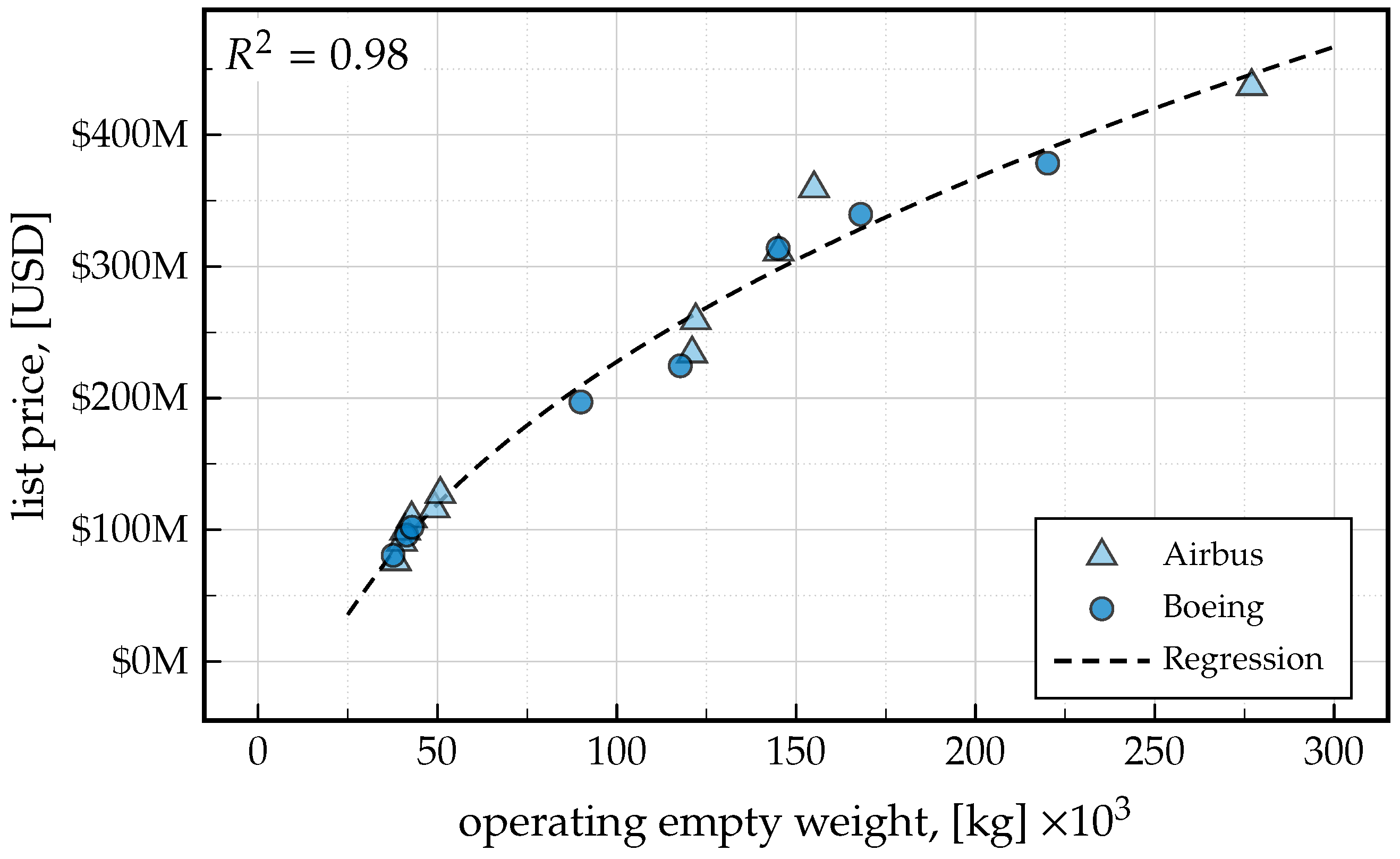
Aircraft Price Estimation: The aircraft price evidently plays a major role for the overall cost-benefit assessment. Its value can be either set manually or estimated automatically. In the latter case, a weight based regression on Airbus and Boeing list prices of 2018 [
49,
50] with
is used.
Figure 6 shows the regression, which has an
of 0.98. As airlines rarely pay the list price [
51], a discount is included, which defaults to 30%.
Financing: If the aircraft is chosen to be bought, either from the operator’s own money or loaned from a bank, the ownership module follows the ordering procedure outlined in Marx et al. [
52]. It involves a downpayment of 3%, a delivery payment of 77%, and the rest distributed equally in annual payments. Insurance is modeled as monthly payments and is calculated using a constant share of the aircraft price (the default is
% per year). Interest is modeled using a loan structure with constant principal payments and declining capital interest payments, as described in Clark [
13]. To avoid a doubled weighting of the aircraft price (i.e., though the purchase and again through the principal payments), only the capital interest payments are taken into account. If the user chooses leasing, only the monthly recurring payments are modeled.
3.3.2. Operations
As its name suggests, the operations module deals with the aircraft’s operation, i.e., it creates and appends all flight events. Based on a flight schedule which is provided by the user, the operations module aims to fly the aircraft as often as possible (current work focuses on the integration of fleet wide operations, which follows a more demand oriented flight scheduling, see Pohya et al. [
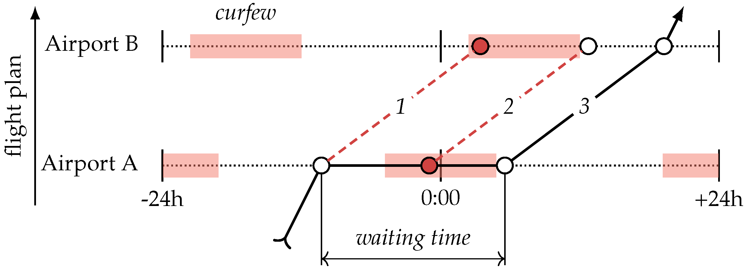
33]). Local airport curfews are taken into consideration, as shown in
Figure 7. In this example, the aircraft lands at Airport A and cannot proceed to Airport B due to an expected landing curfew, shown by path 1. In the second path, a takeoff curfew at Airport A prohibits the aircraft from flying. In the third and final path, both takeoff and landing are allowed. After each path trial, the operations module is exited and the subsequent maintenance module tries to perform due maintenance actions, making use of the waiting time. Recall Code Excerpt A1 for a pseudo code of this process.
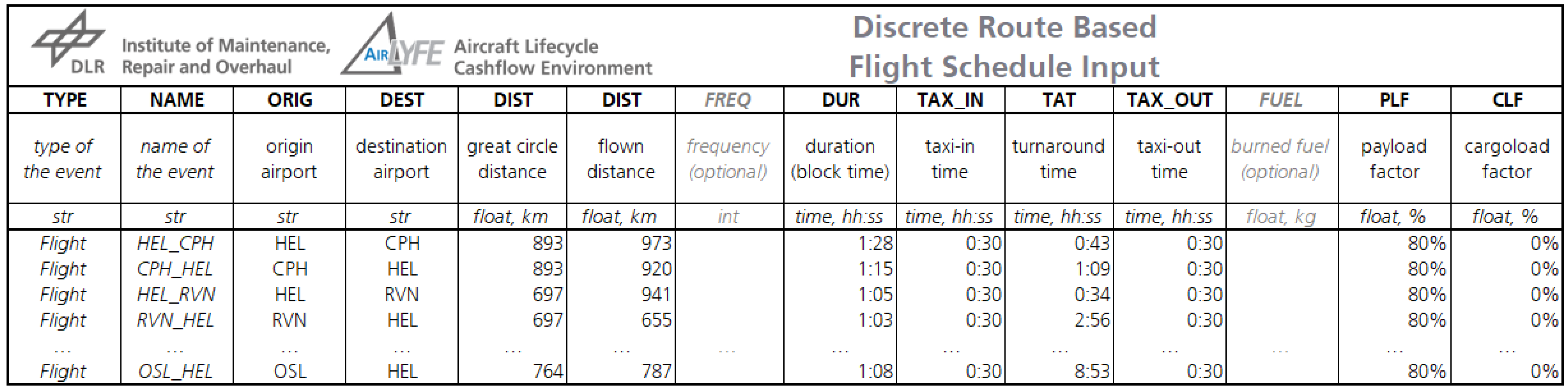
There are two options for users to define the flight plan. Either a particular route schedule is specified (which is to be flown sequentially or in a random manner), or a histogram with average routes and frequencies is provided. The former includes information regarding the origin and destination airports, distances, burned fuel, frequencies, flight durations, taxi and turnaround times, and the passenger and cargo load factor for each route, see
Figure A1 in the
Appendix A. Disruptions in the flight schedule, e.g., through unscheduled maintenance, and their repercussions on the airline’s cost, e.g., through delays and cancellations, are incorporated automatically in LYFE using cost models from Eurocontrol [
53,
54]. As each flight comes with its specific expenditures and revenues, their calculation is explained next.
(a) Flight Revenues
The revenues are comprised of ticket, ancillary, and cargo revenues:
Modeling the revenues directly not only enables the calculation of industry standard investment metrics such as the NPV or Internal Rate of Return (IRR) but also ensures that the economic penalty of missing flights (e.g., due to unforeseen maintenance events) are considered correctly.
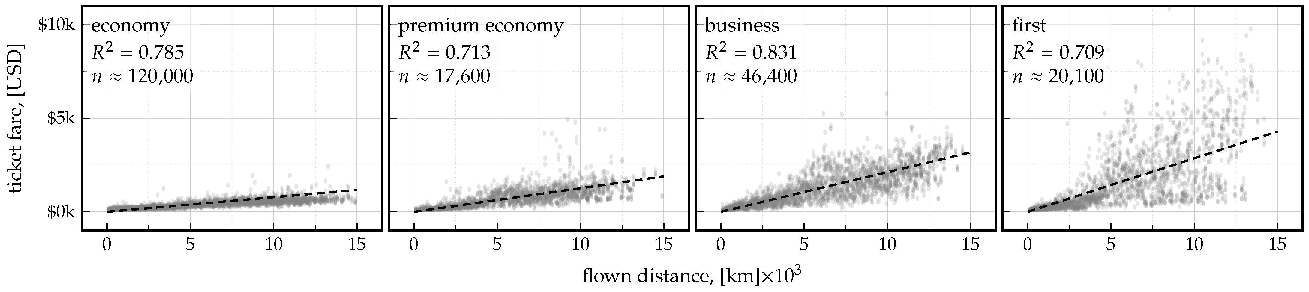
Ticket Revenues: By default, the ticket sales are calculated in AirLYFE through a distance based and seat class differentiated model, based on a regression analysis with
values between 0.7 and 0.83:
The input data were taken from an extract of a commercially available database (See Sabre Data & Analytics [
55]) reflecting the years 2018 to 2019.
Figure 8 depicts the regression for each of the four classes.
Ancillary Revenues: Aside from the ticket prices, ancillary revenues are another income. These include fees associated with excess or heavy bags, extra leg room seating, and onboard services (e.g., food or duty-free sales). Based on a study from IdeaWorks [
56], ancillary revenues are modeled using a specified share of ticket revenues, ranging from 7 to 34% and default to 20%.
Cargo Revenues: As a third income element, the operator may transport some cargo and obtain revenues per carried weight and distance. The internally used value is taken from the DOC method provided in Risse et al. [
20] with
(b) Flight Costs
The costs of each flight can be broken down to:
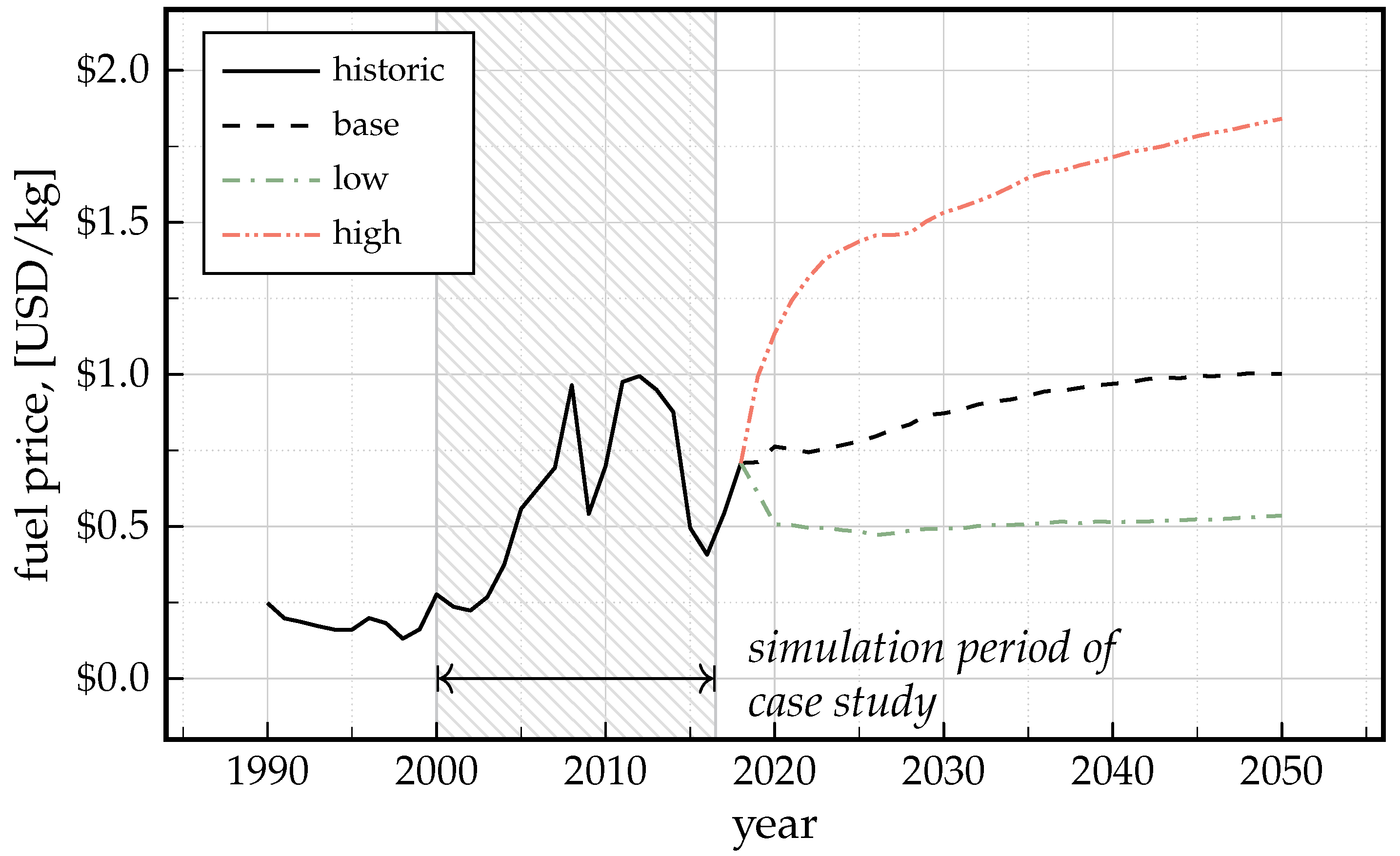
Fuel Cost: Fuel cost plays a major role for many assessment cases and depends on the aircraft’s required fuel burn multiplied by the current fuel price, i.e.,
. AirLYFE provides historical fuel price data dating back to 1990 as well as three scenarios for the future development from 2019 to 2050, which are based on predictions of the US Department of Transportation [
57] considering various macroeconomic assumptions. These are depicted in
Figure 9 where the simulation period of the later performed case study is highlighted.
Navigation and Airport Fees: The cost for Air Navigation Service Providers (ANSP) and airports are calculated using the model from Liebeck et al. [
16], which takes the Maximum TakeoffWeight (MTOW) in tons as input:
Crew Cost: The costs for the cabin and flight crew are calculated using a recreation from an Eurocontrol model [
54]. This involves (a) a determination of how many crew members per aircraft are required, (b) the number of required crew complements, and (c) an estimation of their salary. This model considers not only the number of seats but also the seating class distribution, the type of aircraft (narrowbody or widebody as well as the number of decks), and typical salaries for junior and senior crew members as well as captains and first officers. The user can choose from three available scenarios which represent low-cost, intermediate, and flagship carrier practices. Thus, the crew costs can be expressed as:
3.3.3. Maintenance
The maintenance module deals with scheduled and unscheduled maintenance, both of which are explained below.
(a) Scheduled Maintenance
In the scheduled portion of the maintenance module, the aircraft’s and engine’s health are constantly monitored. Required and recommended maintenance actions are automatically triggered, depending on the location, time, and cost. To do so, either a dedicated maintenance schedule can be provided, or if such information is not available, a regression based method is used. Additionally, users can define systems and components for condition based maintenance. In either case, maintenance costs consist of the cost of material, labor, and fixcost:
The monitoring and triggering process is detailed next, followed by a description of potential input sources.
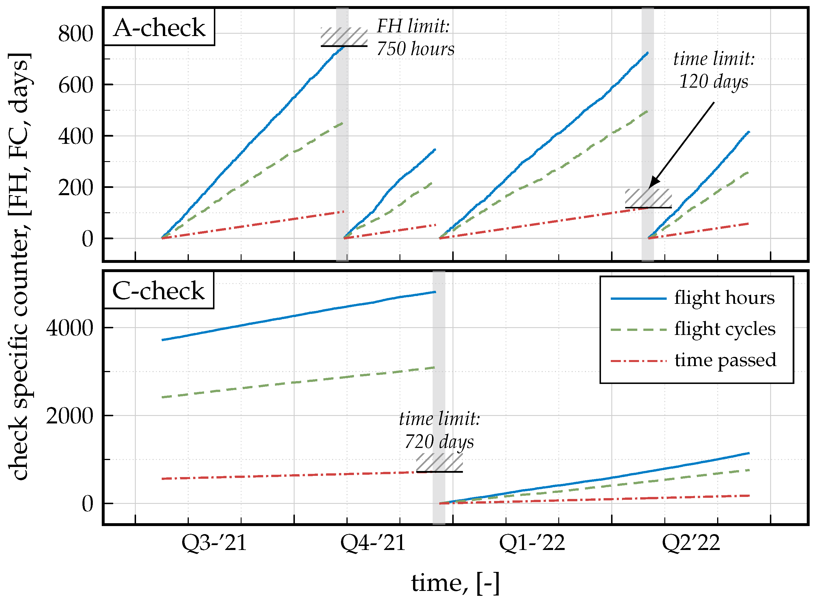
Monitoring and Triggering Process: Per default, the performed flight cycles, flight hours, and age are compared to internally set intervals for each check. If one of these is reached, the corresponding maintenance event is triggered, created, and appended to the calendar. This is illustrated in
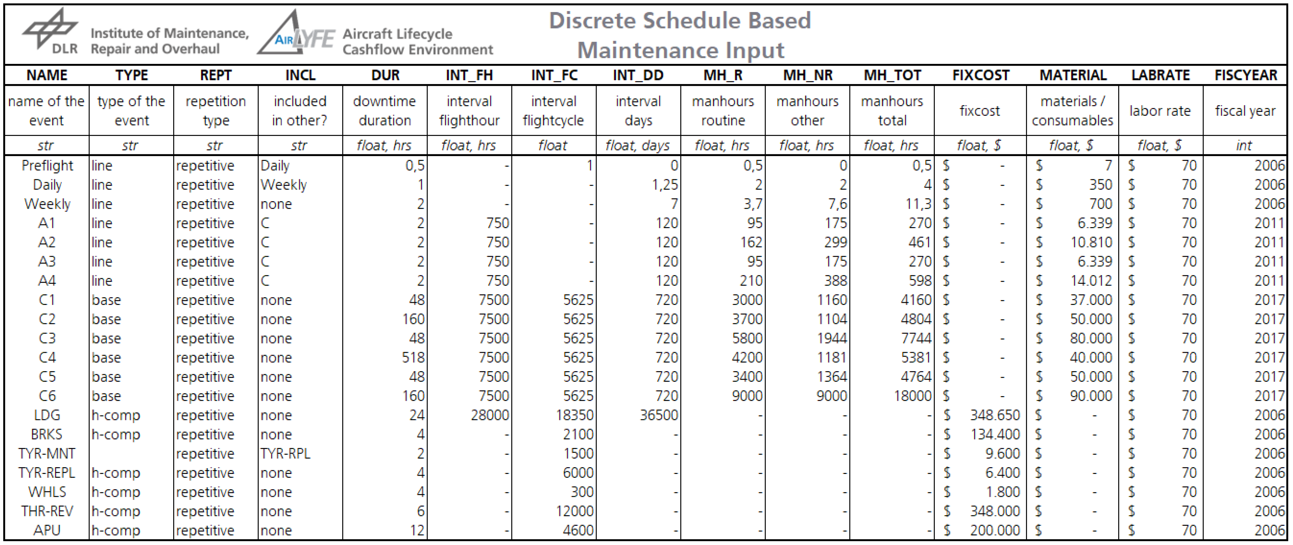
Figure 10 for the A-check (top) and C-check (bottom). Here, the A-check specific counters continuously increase until the flight hours reach their limit of 750 h in Q4 of 2021, triggering the first A-check and resetting the counters. The next A-check is then due in Q2 of 2022, caused by the time interval of 120 days. In between, the counters get reset as well due to a scheduled C-check, which includes the tasks of an A-check in this example. The hierarchy (i.e., which maintenance events include which) is specified freely by the user. Additionally, it is possible to define specific condition degradation behaviors and triggering thresholds for user selected systems and components. The conditions may represent a generic health index or a specific parameter such as the EGT. The condition’s degradation can be defined to increase or decrease in a linear, regressive, or progressive manner with each flight hour, flight cycle, and/or time. This condition based approach complements the regular interval based maintenance schedule.
Sources for the Input Masks: For aircraft that exist and have gone through their first major check cycles, the magazine
Aircraft Commerce regularly publishes articles covering interviews with maintenance organizations and aircraft operators. These include not only a breakdown of the maintenance schedule (e.g., when and which maintenance check is due and what it consists of) but also the associated cost. If such an article is available for the aircraft under investigation, an input mask asks for this schedule and reads the values right from it.
Figure A2 in the
Appendix A shows an excerpt of a check based maintenance file. For new aircraft designs and those that have not been operated long enough to gather sufficient data, AirLYFE provides a fallback mechanism which is based on the DOC method from Refs. [
19,
20]. Since the underlying CER does not differentiate between different discrete maintenance visits but instead provides annual average maintenance cost, they are internally translated to letter checks using typical breakdowns published Aircraft Commerce articles of other aircraft.
(b) Unscheduled Maintenance
Unscheduled maintenance is incorporated with a low level and intermediate level method. Users can choose between these two, depending on the focus of the OoI. The low level method does not model explicit events but instead corrects the scheduled maintenance cost using a factor
f which represents the unscheduled cost portion of labour and material. For this, the age dependent model from IATA is used, which is documented in Suwondo [
58] and takes values from 0.5 at the beginning up to 2.3 at the end of an aircraft’s life. Consequently, the total maintenance cost are
The intermediate alternative of modeling unscheduled maintenance is currently in development and requires a simplified and user specified Master Minimum Equipment List (MMEL), where components under investigation are specified along with their number and dispatch status (i.e., GO, GO IF, or NO GO), and a cross-reference on the maintenance schedule where the respective corrective maintenance action is defined. Randomized failures of these components can then be triggered at any time throughout the simulation according to a user specified failure function.
A third alternative for users to model unscheduled maintenance is to utilize the custom module and code their own failure triggering mechanisms and corrective maintenance actions, which is then integrated into the simulation as described in
Section 3.2.3.
3.3.4. End of Life
By default, the trigger that ends the simulation is the lifetime in years but can be set to any changing parameter within the simulation, e.g., number of flight cycles performed. The standard option is to sell the aircraft for a residual value. The factor for its calculation is determined using a regression model based on data from Clark [
13], which takes the aircraft’s body type and its age
a (in quarters) as input:
The residual value is then calculated using the list price from Equation (
3), i.e.,
. Future work focuses on a more detailed alternative that includes the current condition of the aircraft, following the full-time and half-time valuation in aircraft finance.
3.3.5. Aircraft Performance Database
AirLYFE provides default performance data for 35 different Airbus and Boeing aircraft, based on a commercially available mission calculation tool [
59]. For this, a full factorial simulation of each aircraft was performed, and the outputs (i.e., fuel, time, and emissions) were saved as response surfaces. The inputs cover variations in distance
d and payload
as well as three technology factors, i.e., drag, mass (as a change in Operating Empty Weight (OEW)), and Specific Fuel Consumption (SFC). The input space for the payload and range was mapped with 144 samples (12 each, from min to max), whereas the technology factor space was covered with 1331 samples (11 each, from
to
). This is shown in
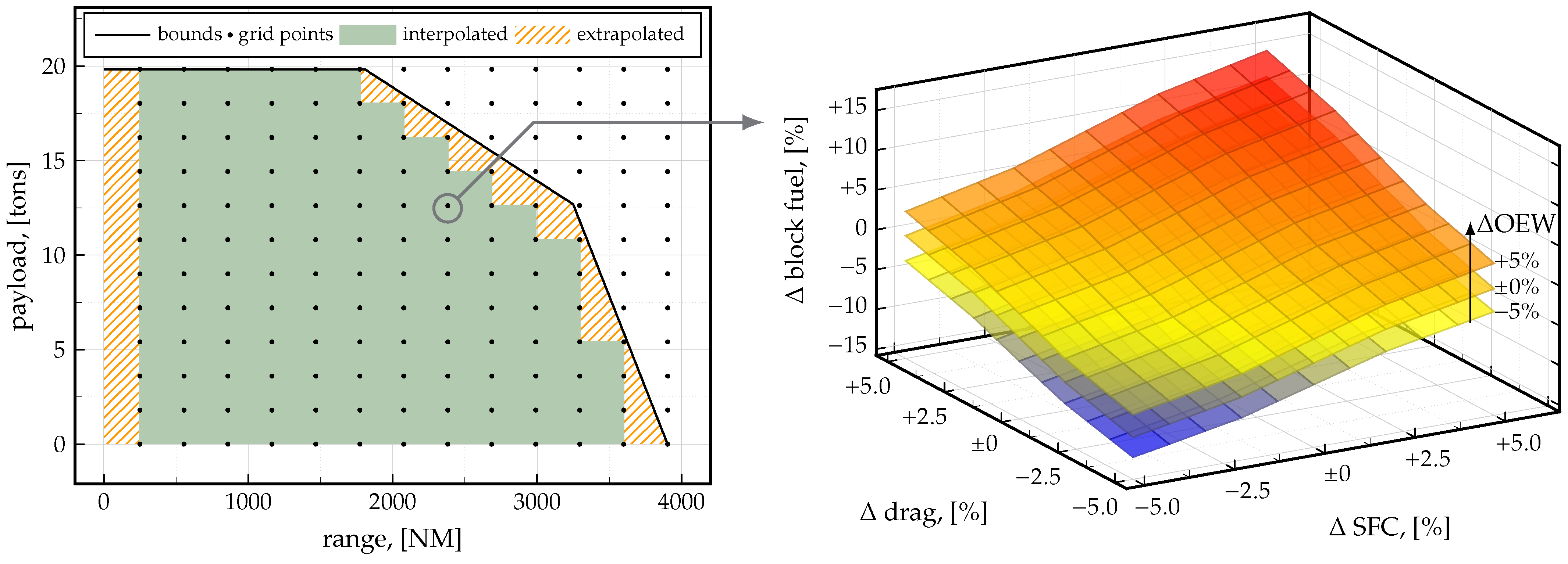
Figure 11, where the left plot depicts the payload-range boundary, grid points, and the areas of inter- and extrapolation. The right plot represents the technology factor mapping which is behind each of the grid points. With these response surfaces, AirLYFE calculates the fuel burn, flight time, and emissions with a multi-linear interpolation in the five input dimensions [
60], i.e.,
This performance model, which is attached to each aircraft object, allows users to quickly and easily simulate the impact of a variety of technologies. Furthermore, the impact of aircraft and engine deterioration can be modeled by gradually increasing the drag or SFC, e.g., by a certain percentage per flight. Alternatively to this approach, it is possible to precalculate the required fuel burn per mission and feed this information to the operational schedule shown in
Figure A1.
3.3.6. Airport and Weather Database
The airport database that was compiled for LYFE comprises about 6000 different airports worldwide and includes information (all gathered from publicly available sources) such as:
The latitude and longitude (e.g., for calculating great circle distances);
The timezone and local curfews (required for the flight schedule);
The runway altitude as well as representative weather information including wind speed, local day and night temperatures, surface pressure, and rainfall.
The weather information includes mean values and standard deviations for each month, enabling the generation of random but representative weather information. For this database, publicly available climate data (i.e., European Centre for Medium Range Weather Forecasts (ECMWF) [
61]) from 2017 to 2019 were analyzed on every airport coordinate and processed.
Figure 12 shows a map of the available airports and their average daytime temperature in July for illustration purposes. These weather parameters are not actively used per default but are available for users if they wish to model, for instance, a temperature dependent degradation behavior, as for example in Wehrspohn et al. [
62].
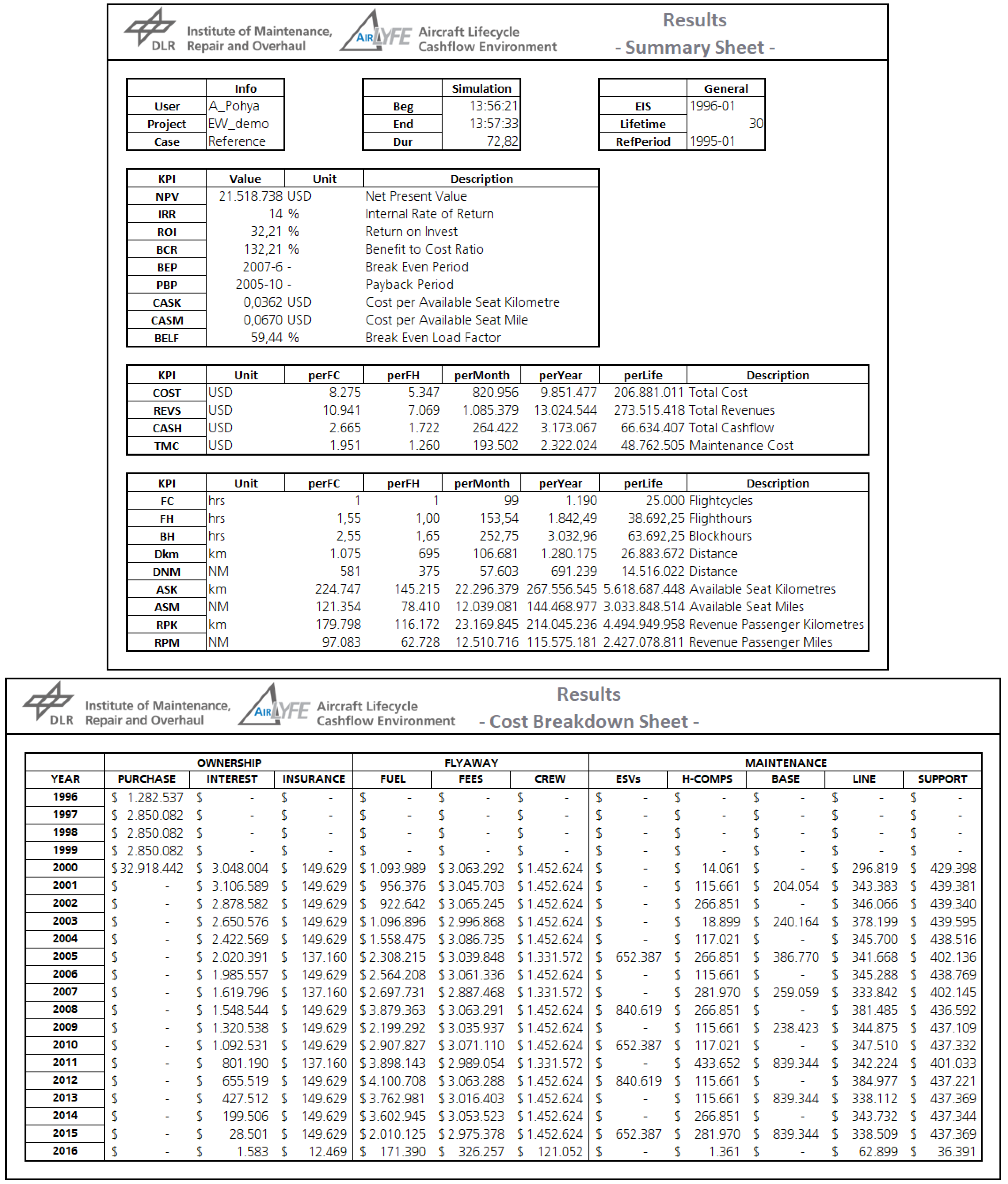
3.3.7. Economics and Report
At the end of a simulation, an Excel based report is generated. In here, different economic metrics as well as statistical Key Performance Indicators (KPIs) are calculated. These include, but are not limited to, the NPV, IRR, LCC, the return on invest, the benefit-cost-ratio, cost per available seat mile, break even load factor, and KPI breakdowns per flight hour and flight cycle. Out of these, the NPV and IRR are the most frequent used in investment decision making [
13,
63]. The former takes the annual cash flow (
) as well as the time value of money (using a discount rate
r) into account and is defined as
These economic metrics and operational statistics are summarized in the first sheet. Additional sheets include periodic breakdowns (both annually and monthly), as well as diagrams for visualization and sanity check purposes.
Figure A3 in the
Appendix A depicts the summary sheet with generic information in the upper table, followed by the annual monetary breakdowns in the lower table.
4. Case Study
Due to the variety of available features, a single use case will not be able to show LYFE’s capabilities in their entirety. However, a demonstrative case study can facilitate the understanding about the default modules and methods as well as show a typical situation where the framework is customized. For this, the on-wing maintenance action of engine wash is assessed on an Airbus A321 type of aircraft with respect to its impact on the operational and economic value. This section begins with providing some background information on this topic. Next, the methodology for the assessment is presented, including a description of the custom module which contains decision making algorithm. Finally, the results in terms of improved fuel efficiency and decrease of operating cost are shown.
4.1. Background and Study Assumptions
Readers that are unfamiliar with aircraft engine maintenance and engine wash find a brief overview here. Furthermore, the underlying assumptions regarding the aircraft and engine under study are explained in this section. It is highlighted that this case study serves demonstrative and representative purposes and was performed using only publicly available information.
4.1.1. Basics and Incentive
Aircraft engines are a highly complex and expensive asset which represent about a fifth of an aircraft’s price. Their maintenance, which constitutes for about 35 to 40% of the airline’s Direct Maintenance Cost (DMC), can be divided into on-wing and off-wing measures. Off-wing maintenance are usually ESVs, where the engines receive, depending on the workscope, a partial or full overhaul [
64,
65]. These ESVs are typically scheduled when either the monitored health of the engine approaches a critical value or the RUL of Life Limited Parts (LLPs) is depleted [
66]. The former is typically represented by the EGT, which increases with the engine’s level of deterioration. Manufacturers specify an engine-specific upper limit (EGT
) which must not be exceeded due to thermal stress reasons. ESVs can cost several million dollars and last 4–6 weeks. Considering the high airworthiness requirements, operators thus strive to keep their engines in good condition at all times. One additional measure to do is the on-wing engine wash, where water and cleansing additives are pumped into the engine’s intake. Several Maintenance, Repair, and Overhaul (MRO) providers and engine manufacturers offer this procedure, such as Lufthansa Technik [
67], General Electric (GE) [
68], or Pratt & Whitney [
69]. Engine Wash (EW) removes accumulated dirt, improves fuel efficiency, and decreases EGT up to 15 °C [
64]. It is typically performed for one engine at a time for safety reasons and lasts one to four hours, depending on the provider. The overall effectiveness of EW depends on multiple factors. Apart from their cost, they include:
The timing, as dirt has to be accumulated first, before it can be washed away.
The sensitivity of the engine’s SFC on the EGT increase, as this determines the resulting fuel burn savings. This is cited to be within the range of 0.07 [
70,
71] to 0.1% [
30] of SFC increase per °C of EGT.
The fuel price, which determines the potential cost savings an EW can bring.
The value of additional time on wing, since the partial restoration of EGT can lead to a delay of ESV.
Interested readers are refered to Ackert [
64,
65] and Hutter [
70] for further literature on engine deterioration and maintenance.
4.1.2. Assumptions and Simplifications
For this study, we have chosen the CFM56-5B3 engine with a simulation lifetime of
EFC. For an operational input, the annual flight schedule of an A321-211 from Finnair based in Helsinki was used. This schedule consists of 1746 flights (53 unique routes), has an average Engine Flight Hour (EFH)/Engine Flight Cycle (EFC) ratio of
, and is depicted in
Figure 13.
The maintenance schedule for the airframe was built based on an Aircraft Commerce article [
72] and consists of regular transit, pre-flight, daily and weekly checks for line maintenance, and equalized A-checks and C-checks that are repeated in an six-cycle manner for base maintenance. Heavy component maintenance and recurring fees for rotables were also considered. This input schedule is the one shown in
Figure A2 in the
Appendix A. The engine maintenance was modeled with automatically triggered ESVs. If either the Exhaust Gas Temperature Margin (EGTM) approaches zero or the RUL of one of the LLPs falls below 1% of the LLP margin, the next ESV at the maintenance base is scheduled. According to Aircraft commerce [
66,
72], CFM56-5B operators often follow an alternating ESV workscope strategy, where the core receives a restoration during the first ESV, and a full overhaul is performed at the second. This was incorporated into the maintenance input, along with the four groups of LLPs lives (High Pressure Turbine (HPT), High Pressure Compressor (HPC), fan, and Low Pressure Turbine (LPT)) and their associated replacement cost.
For the Exhaust Gas Temperature Increase (EGTI), a simplified EFC dependent model was created, based on interviews of MRO providers [
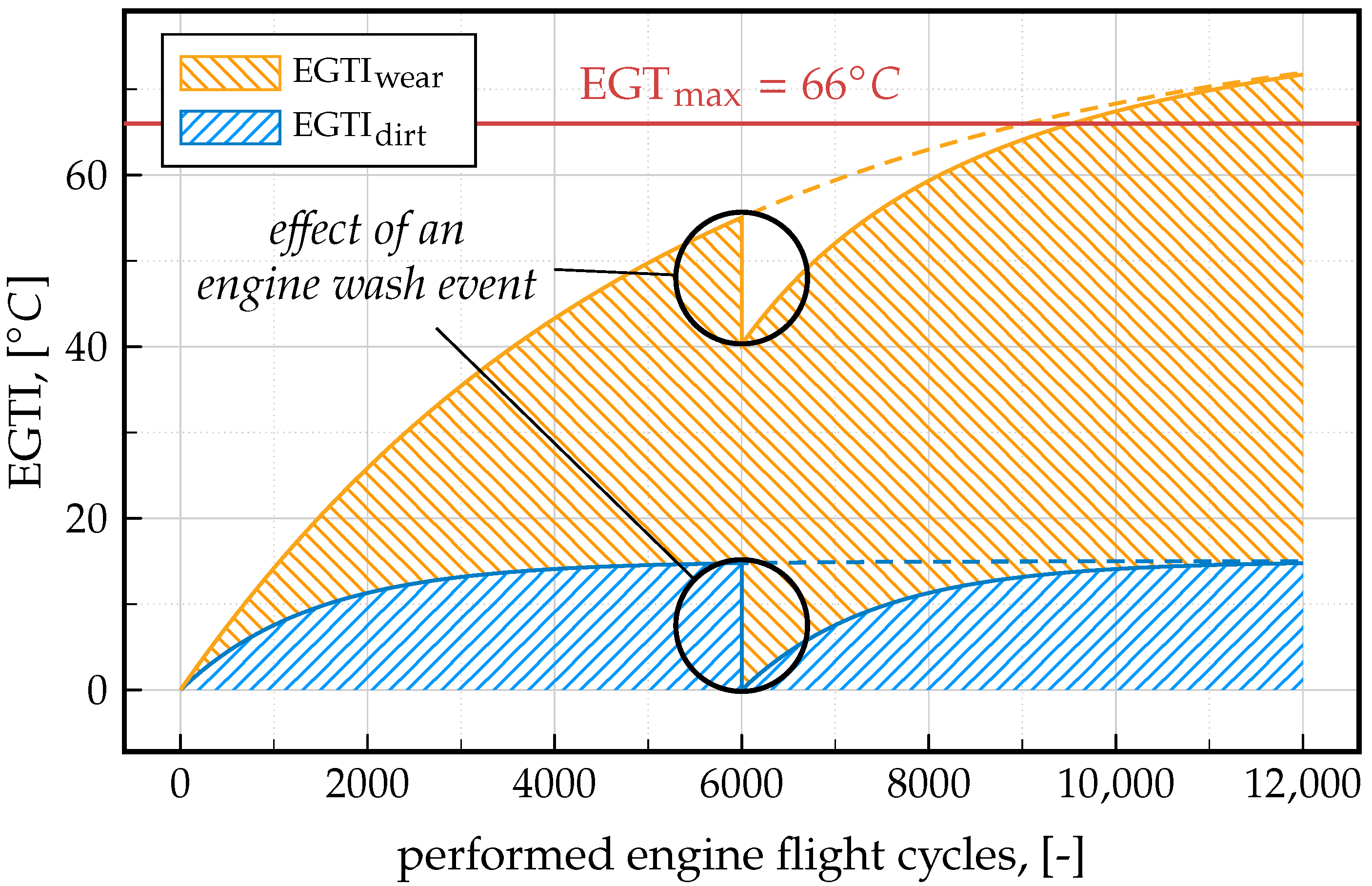
66]. This increase was divided into two parts, one due to an increase of wear and tear and one due to the accumulation of dirt. The shape of the latter was modeled without any available data, solely based on an educated guess, and is visualized in
Figure 14 (blue hatched area), along with the wear induced EGTI (orange hatched area) and the impact of an engine wash. Note that only the dirt induced EGTI is removed, and the wear induced EGTI stays unaffected. The mathematical representation is given in Equations (15) and (16).
For the translation of EGTI to fuel burn, a value of 0.01% SFC increase per °C of EGTI was used. Furthermore, the EGTM restoration after an ESV was implemented assuming that a core restoration reaches 60% and a full overhaul 80% of the original margin of 66 °C. Other assumptions regarding this study are:
The engines do not switch the aircraft type (e.g., from an A321 to an A320 or A319 after downrating the engine) during their life.
One engine wash event costs $3000 (including material and labor) and has a duration of two hours.
Only one aircraft with one set of engines is simulated. Engine fleet effects (e.g., spare parts management) are neglected.
Unless otherwise specified, the default methods for calculating cost and revenues are used.
The entry into service of the aircraft is January 2000.
4.2. Methodology and Module Modification
The study comprises two simulations. The first serves as a reference and does not take any EWs into account. In the second simulation, EWs are triggered by an optimization algorithm, which is implemented into the custom module of AirLYFE. The overall effectiveness is then compared to the reference case using the total EW cost and saved fuel cost as economic KPIs and the fuel efficiency improvements as an operational metric.
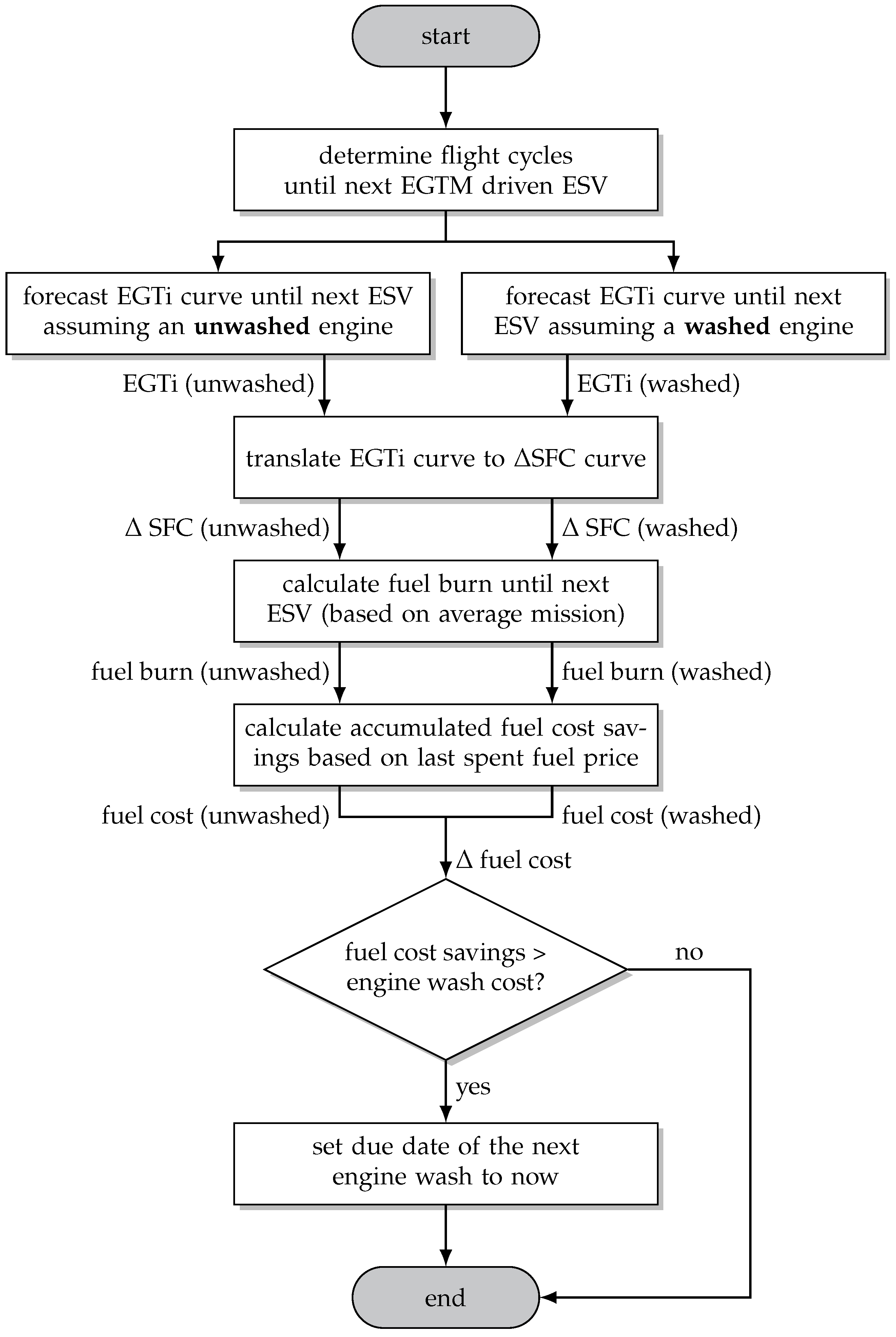
The implemented algorithm triggers an engine wash event only when the predicted fuel savings outweigh the cost of the cleaning. As
Figure 15 shows, the first step is to predict the future engine health based on its current state and forecast the RUL, i.e., the number of flight cycles left until an ESV is triggered. Then, two EGTI predictions are performed: one assuming that no EW is scheduled, and the other assumes an EW event before the next flight. Both curves are then translated to
SFC forecasts. For the next step, the average flown mission (in terms of payload and range) is fed to the aircraft performance model, along with the two
SFC vectors. This results in two vectors for the fuel burn, one with a washed and the other with an unwashed engine. These are then transformed to absolute fuel cost savings using the last paid fuel price. If these fuel cost savings are greater than the cost for an engine wash, it will be scheduled for the next opportunity. It should be noted that the average flown mission was chosen intentionally over using the actual future flight schedule in order to be slightly more realistic in the prediction. The same applies for the underlying fuel price, i.e., although the future fuel price is theoretically available, the latest paid price is used in the decision making, intentionally introducing an imperfection in the forecast.
A pseudo code of the
custom module, which also includes the engine deterioration specified by Equations (15) and (16) is given in Code Excerpt A3 in the
Appendix B. To speed up the computational time, the EGTI is precalculated in the
init() function and used as a lookup table in the
main() function. This also contains the triggering mechanism of the ESVs and the decision of workscope, i.e., which LLPs to include.
Apart from the custom module, only the report generation has been modified to capture repeated snapshots of the engine’s EGT and fuel efficiency.
4.3. Results
The results of the demonstrative study are also divided into two categories: those of the reference simulation (without any engine cleaning procedures) and those with the fuel cost optimization strategy in place. Note that all monetary values refer to the fiscal year 2021.
4.3.1. Reference Case (No Engine Wash)
In order to facilitate the interpretation of assessment results, the reference to which the study case is compared has to be well understood. Therefore, its overall economic results are presented first, followed by a more detailed look into the unwashed engines’ condition and fuel performance.
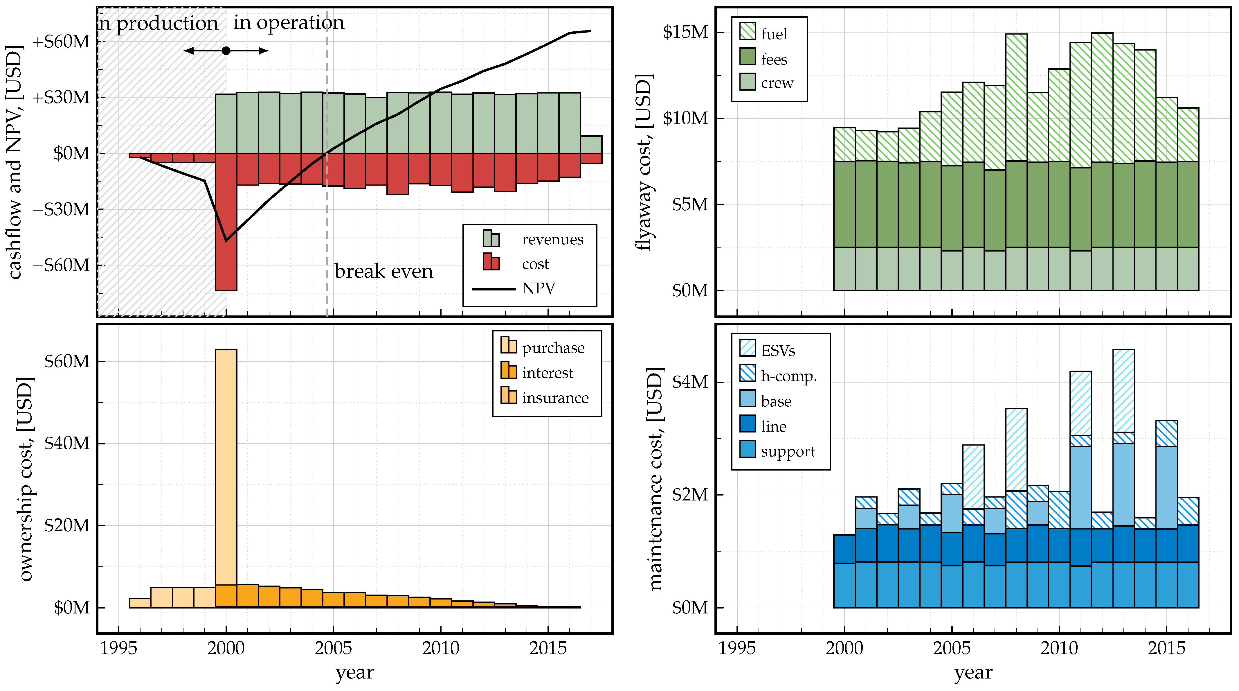
Figure 16 (top left) shows the cashflow in terms of the aircraft’s annual revenues and expenditures as well as the NPV from 1996 (where the aircraft is ordered) until 2014 (where the 25,000 flight cycle limit terminates the simulation). Three typical periods can be distinguished: (a) the non-operating phase in the first few years, where the aircraft is in production and first payments are due but no revenues are generated (1996–2000), (b) the first part of the operating phase, where the aircraft is flying and creating a positive cash flow but the NPV is still negative due to the previous financial burden (2000–2005), and (c) the second part of the operating phase, where the NPV is positive and the aircraft is adding economic value for the operator. In the final year, the costs and revenues are reduced significantly due to the fact that the simulation ends before the end of 2017, i.e., this year is not fully exploited, leading to a final NPV of
$M. The other three plots of
Figure 16 provide a more detailed breakdown of the operating cost. The ownership costs (bottom left) show, apart from the dominating purchase cost, the declining payments for capital interest and the constant and comparatively low insurance cost. The flyaway costs (top right) comprise crew expenses, fees, and fuel cost. The constant character of the navigation and airport charges indicates a fairly constant annual utilization. The high variation of the fuel cost can be explained by the historic fuel price change from initially
$/kg in 2000 to
$1/kg between 2011 and 2014 and back to
$/kg between 2015 and 2017 (see
Figure 9). The annual maintenance cost breakdown (bottom right) reveals a highly fluctuating behavior, with a honeymoon phase (low cost due to the aircraft being new) in the beginning and several distinct peaks in the mature phase. These peaks are due to heavy component maintenance, larger base checks, and/or ESVs.
With the focus of the present study on EW, the engines’ condition is of primary interest.
Figure 17 shows the course of the monitored parameters EGT (top) and fuel efficiency (bottom). As the top plot shows, the regressive EGTI triggers the first ESV at about 9000 flight cycles. The performed workscope restores
°C of EGTM. The second ESV at 12,540 flight cycles, which is again triggered by the consumed EGTM, is able to restore
°C of EGTM (due to the full overhaul workscope) and additionally replaces the LLPs of the HPT section. The subsequent three ESVs are triggered by the LLPs of the HPC, fan and LPT section (in this order). The EGT at these ESVs is fairly close to the EGT
, indicating an overall efficient engine maintenance schedule. Its restoration is slightly lower since it is assumed that only a certain condition of the overhauled engine can be reached. In the bottom plot, the fuel efficiency
shows a spread from 2.5 to
(L/pax/100 km), originating from (a) the wide spread of flown distances (ranging from 360 to 1820 NM) and (b) the effect of the engine deterioration on SFC. Depending on the performed workscope, an ESV leads to an improvement of
of 0.1 to
L/pax/100 km (≈3 to 6%, depending on the route). It should be noted that the occurrence of ESVs, their cause (EGT or LLP), and the resulting fuel efficiency values are well in line with the practice reported by A321 and CFM56-5B3 operators in Aircraft Commerce [
72].
4.3.2. Fuel Cost Optimized Use of EW
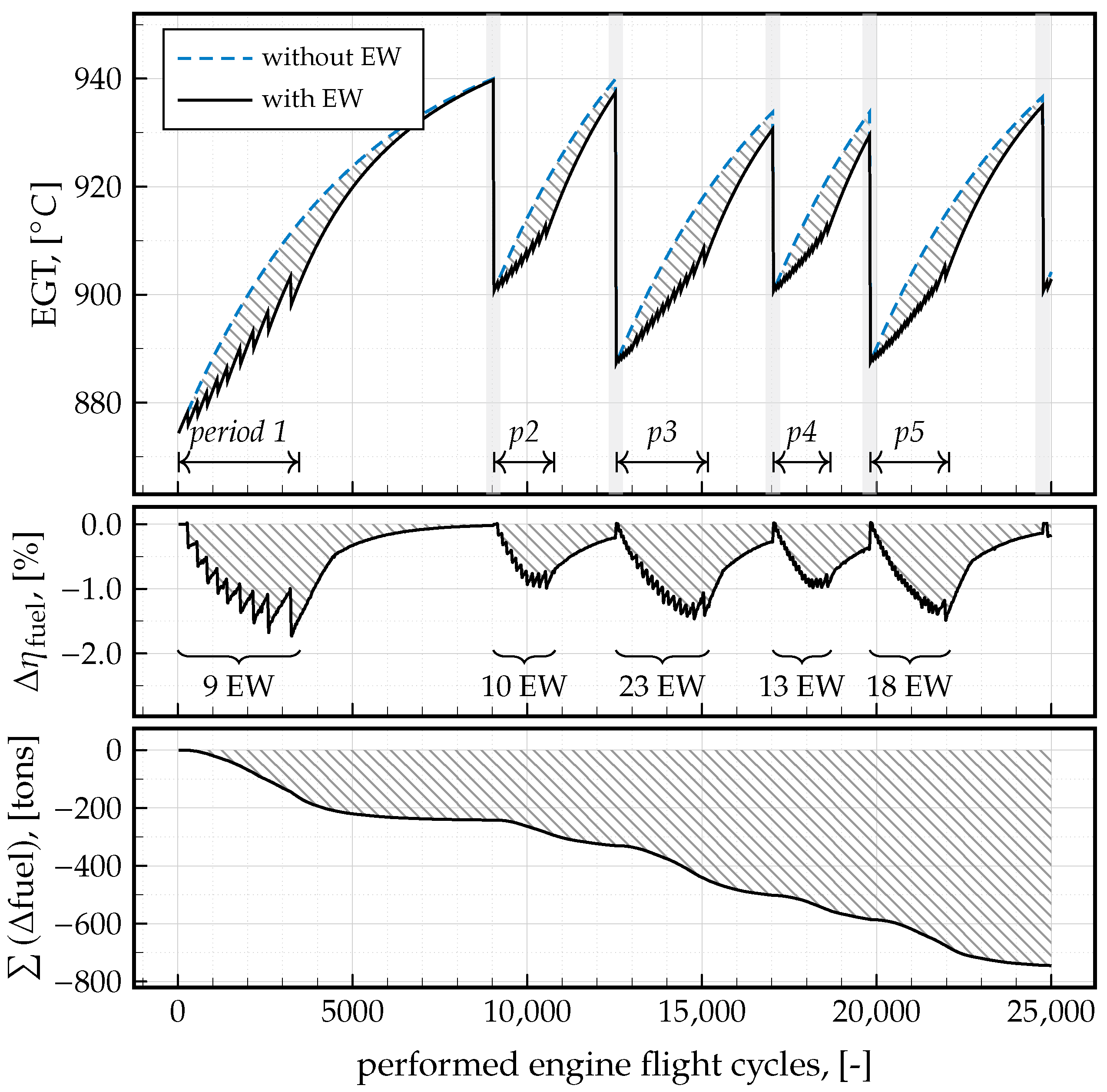
The effect of the automatically triggered EWs on the engine’s health, fuel efficiency and overall resulting fuel savings can be seen in
Figure 18. In total, the optimization algorithm schedules 216 cleaning events, distributed into five periods. The number of EWs per period correlates with the fluctuating fuel price and is lower in the beginning (i.e., between 0 and 3200 EFC, where 10 EW events are triggered at a fuel price of
$0.25 per kg) and higher in the later phases (e.g., between 17,000 and 20,000 EFC, where 23 EW events are triggered at
$1 per kg). This leads to an improved but fluctuating fuel efficiency improvement as shown in the center plot, ranging from zero to
%. Accumulated throughout the simulation, this improvement leads to fuel and CO
savings of 780 and 2500 tons, respectively (these are not shown but can be approximated well with
). As the spikes in EGT and
show, the optimization algorithm tends to schedule cleaning events in the beginning of each period. The reason for this is that with each performed EFC, the prognostic horizon (i.e., number of EFC until the next ESV) decreases, which in turn leads to smaller potential fuel savings that need to outweigh the EW cost. In other words, it is not useful to perform an EW shortly before an ESV, as the EGT will be restored soon anyway.
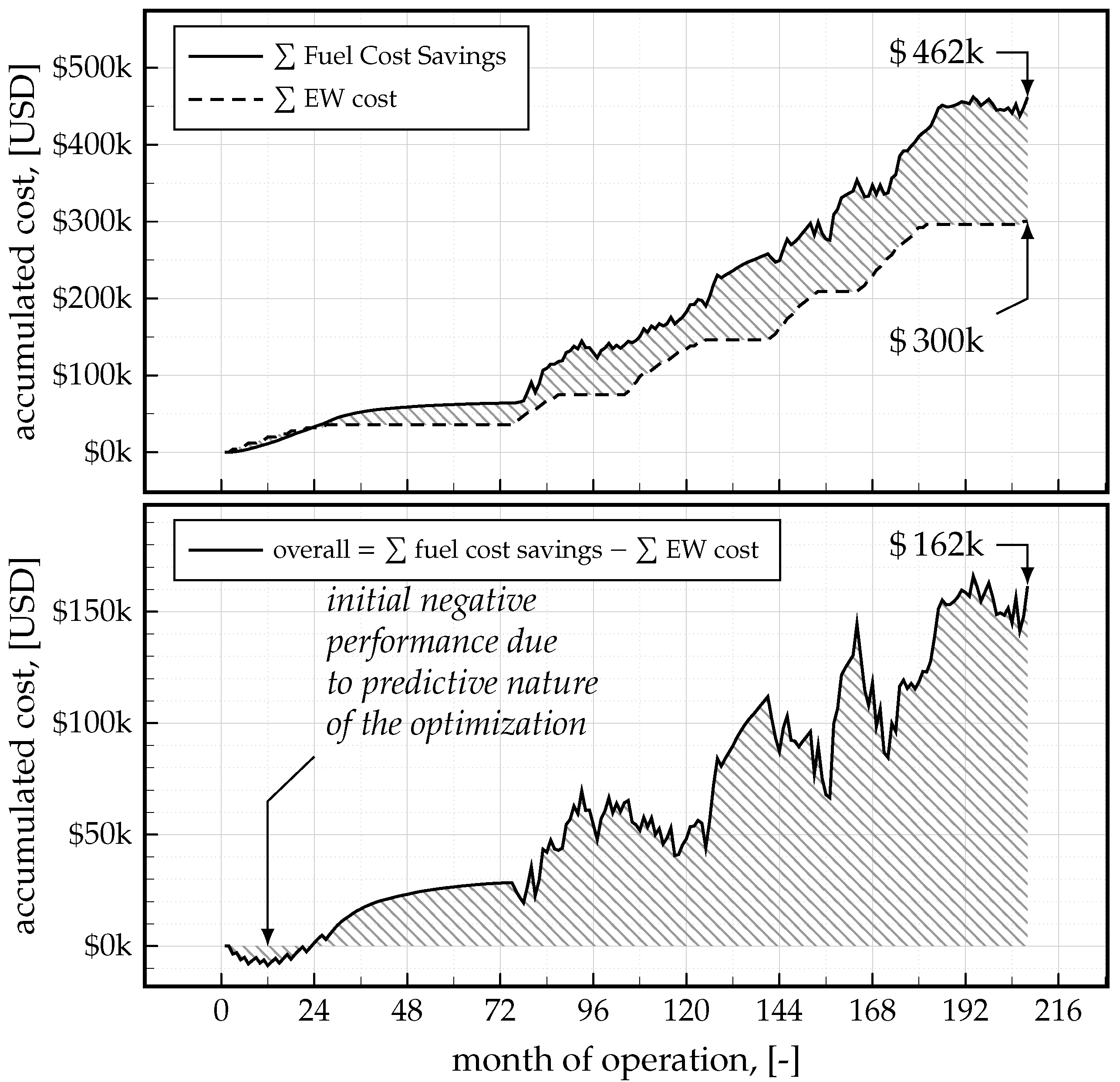
As for the impact of EW on airline economics,
Figure 19 reveals that a total of
$300k is spent for the cleaning events, while
$462k are saved through the improved fuel burn, leaving an added value of
$162k for the operator. As the bottom plot shows, the predictive nature of the optimization algorithm leads to an initially negative economic performance, as the accumulated fuel cost savings do not yet compensate the accumulated EW cost. After about two years and 2900 EFC, the profitable phase begins, which shows increasing overall operating cost savings. The fluctuating behavior is caused by several factors. For one, the scheduling process does not forecast the actual flown schedule but extrapolates it in a simplified manner from the average distance and utilization, leading to slightly different savings than expected. Furthermore, the fuel price development is chosen to be unknown to the algorithm (as it more accurately represents the reality), which also affects the anticipated cost savings.
Despite being a demonstrative and simplified assessment, this example provides meaningful insights, explainable repercussions, and directions for further studies in this area. The latter may include the effects of EW on the subsequent ESV workscope, a more detailed modeling approach for the EGTI, alternative optimization algorithms, or the systematic treatment of uncertainties in the prognosis. This also includes a validation of the EGTI models and its repercussions on the SFC, fuel burn, and ultimately cost savings. In light of the presented LYFE framework, this example aimed to show the advantages of the available aircraft performance databases (where no additional fuel burn calculations were required) as well as the usefulness of the customization interfaces, where a user-written and study specific module (including the engine degradation model and optimization algorithm) was seamlessly incorporated with little effort, while no alterations of the source code or general structure of LYFE were necessary.
5. Summary and Outlook
This paper presented a generic assessment framework for aeronautical applications named Life Cycle Cash Flow Environment (LYFE). LYFE aims to replace the conventional and prevalent Cost Estimation Relationship based methods, which suffer from a range of limitations. Based on a discrete event simulation, the presented tool is capable of capturing primary (i.e., immediate) and secondary (i.e., time delayed) effects of various changes in a product’s life cycle. This includes, but is not limited to, the integration of physical technologies, the degradation of structures and systems, specific maintenance actions, and operational decision making. The modular structure and customizable nature of the framework facilitates this wide range of applicability. For demonstrative purposes, the process of on-wing engine cleaning was evaluated on an CFM56-5B engine of an Airbus A321 aircraft. This included a custom module which contained an engine deterioration model and a predictive Engine Wash scheduling algorithm that aimed to minimize operating cost. Hereby, interrelations between the engine’s health, its manifestation in the Specific Fuel Consumption, the partial Exhaust Gas Temperature restoration capabilities of Engine Washes and Engine Shop Visits, and the exchange of Life Limited Parts were considered in the assessment. The results have revealed valuable insights and potential directions for future work in this area. Apart from that, the general future LYFE development will focus on improving user friendliness and further detailing the default modules, with the intent of being the standardized and publicly available cost–benefit tool for aeronautical product evaluations.


