Online Model-Based Remaining-Useful-Life Prognostics for Aircraft Cooling Units Using Time-Warping Degradation Clustering

Abstract

Remaining-useful-life prognostics for aircraft components are central for efficient and robust aircraft maintenance. In this paper, we propose an end-to-end approach to obtain online, model-based remaining-useful-life prognostics by learning from clusters of components with similar degradation trends. Time-series degradation measurements are first clustered using dynamic time-warping. For each cluster, a degradation model and a corresponding failure threshold are proposed. These cluster-specific degradation models, together with a particle filtering algorithm, are further used to obtain online remaining-useful-life prognostics. As a case study, we consider the operational data of several cooling units originating from a fleet of aircraft. The cooling units are clustered based on their degradation trends and remaining-useful-life prognostics are obtained in an online manner. In general, this approach provides support for intelligent aircraft maintenance where the analysis of cluster-specific component degradation models is integrated into the predictive maintenance process.

1. Introduction

Globally, aircraft maintenance, repair and overhaul (MRO) costs account for $9\%$ of the total airline operational costs [1]. To reduce these maintenance costs and, in particular, to reduce the costs of the maintenance needed in the case of an unexpected failure, MROs benefit from predictive maintenance. Here, the analysis of sensor health-monitoring data for aircraft components is central. By analyzing this data, the aim is to make predictions about the remaining-useful-life (RUL) of the components.

In the past, several RUL prognostic methodologies have been developed [2], mainly using data-driven and model-based approaches. Examples of data-driven methodologies for RUL prediction are neural networks [3,4] and neural fuzzy networks and recurrent neural networks [5,6]. Model-based RUL prediction methodologies have employed Wiener processes [7,8], Kalman filters [9], particle filtering [10], physics-based models [11,12], and Markov models [13].

In most such studies, an inherent assumption is made that there is only one degradation mechanism or trend that governs the failure of components [14]. However, given that systems are often complex, with multiple interconnected components, and given that each component is subject to various operational and environmental factors, it is expected that the degradation of components follows more than one failure mechanism or trend [14,15]. As such, several degradation models should be integrated into the RUL prediction methodology, in order to capture the various degradation trends toward component failure.

Only a limited amount of studies developed RUL predictions using multiple degradation models. Data-driven approaches with multiple degradation models were considered in [16,17]. In [16], a Long Short-Term Neural Network was developed such that degradation patterns under multiple operational conditions and belonging to several fault modes were detected. With this approach, the RUL of aircraft engines was estimated.

In [17], a deep learning approach was combined with a genetic algorithm to predict the RUL of aircraft engines operating under multiple conditions and failing under several fault modes. Machine-learning approaches, however, are often seen by aircraft maintenance practitioners as “black-boxes” [6]. This is an obstacle for the implementation of purely data-driven prognostic methods in practice [18]. In this paper, we, therefore, focus on a model-based prognostic approach that considers multiple models to capture the degradation trends of components.

Model-based RUL prognostic approaches that incorporate multiple degradation models and fault modes were considered in [14,19,20,21,22,23]. In [19], four physics-based failure models of subsea pipelines were incorporated into one dynamic Bayesian network. In [14], the authors considered multiple resistance degradations for batteries, each with its own degradation trend. With these degradation models and a particle filtering algorithm, the authors predicted the RUL of batteries. A switching Kalman filter to model multiple degradation trends within one degradation process was used in [22,23] for bearings and in [20] for aircraft engines. In contrast to these studies, where multiple degradation models are integrated in one comprehensive degradation model, we first cluster the degradation trends of components and propose cluster-specific degradation models. In this way, different components are associated with different degradation models.

For model-based RUL prognostic methods, two frequently considered models are the exponential and the linear degradation models [2,24]. Linear degradation models were developed in [25,26,27,28]. In [25], a linear model with Brownian drift and random shocks, together with a particle filtering algorithm, was used to estimate the RUL of milling machines. A linear degradation model was also used in [26] for batteries, in [27] for aircraft engines, and in [28] for engine bleed valves.

Exponential degradation models were used in [29,30,31,32,33]. An exponential model was used together with a particle filtering algorithm to predict the RUL of bearings in [29], and to predict the RUL of batteries in [30]. An exponential model for the degradation of bearings was also considered in [31], for batteries in [32], and for railway turnout systems in [33]. Similarly, in this paper, we consider clusters of components that degrade according to a linear or an exponential model.

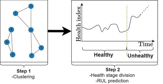
In this paper, we propose an end-to-end approach to obtain online, model-based RUL prognostics for aircraft components by exploiting the knowledge obtained from clusters of component degradation trends. First, using sensor monitoring data, we construct a health indicator, which is used to diagnose components as being healthy or unhealthy. As soon as a component is diagnosed as unhealthy, a cluster-specific degradation model is selected for this component based on a dynamic time-warping clustering of a library of health indicators. These degradation models, together with a particle filtering algorithm, are further used to obtain RUL prognostics.

We illustrate our approach for the case of several aircraft Cooling Units, originating from a fleet of aircraft. We consider operational aircraft data, i.e., the sensor measurements were collected during actual operation of the aircraft. The results show that our proposed cluster-based RUL prognostics approach was robust and consistent across multiple components.

The main contributions of this paper are as follows:

(i)

We propose an end-to-end methodology from sensor measurements to diagnostics of a component as healthy or unhealthy to RUL prognostics. Using a health indicator, a component is diagnosed as healthy or unhealthy. Once a component reaches the unhealthy stage, a degradation model is selected based on the similarity between the degradation trend of this component and clusters of a library of health indicators. This approach exploits the potential learning from degradation trends of other components.

(ii)

We consider multiple degradation models. A generic clustering method of the degradation of components is proposed. Each obtained cluster is associated with one degradation model and a corresponding failure threshold.

(iii)

Our proposed approach is illustrated using operational aircraft data, i.e., the sensor measurements were collected during the actual operation of the aircraft. In general, case studies are often conducted with simulated data or sensor data generated in a laboratory, which may not be as noisy as the aircraft operational data.

The remainder of this paper is organized as follows. In Section 2, we provide a methodology for online, model-based RUL prognostics using dynamic time-warping and a particle filtering algorithm. For time-warping, we consider several, same-type components, which are clustered based on the similarity between their degradation trends. In Section 3, we illustrate our methodology for several aircraft cooling units. Section 4 provides our conclusions and recommendations for further research.

2. Online, Model-Based Rul Prognostics for Multiple Components

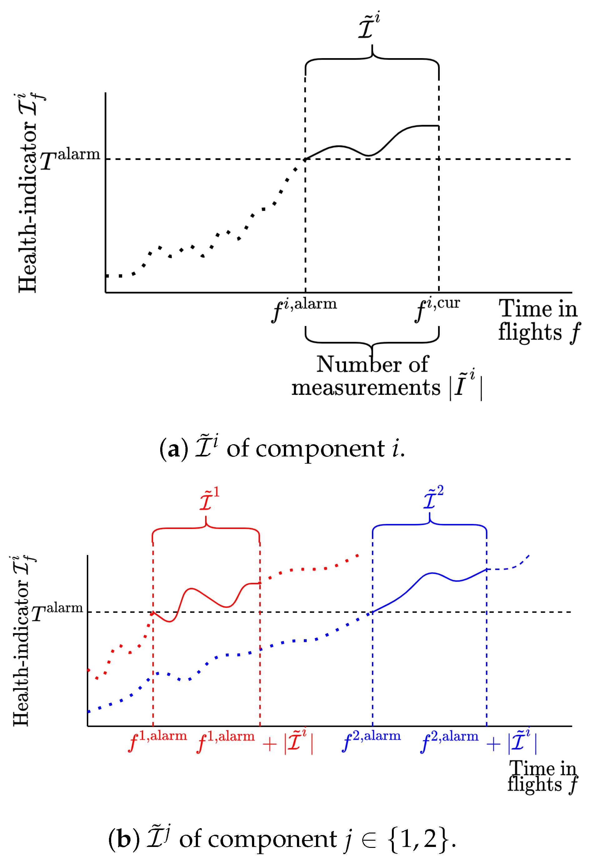
In this section, we provide an approach to obtain online RUL prognostics for aircraft components. We first construct a health indicator from the sensor monitoring data. Based on this health indicator, we online diagnose a component as being healthy or unhealthy (step 1). Once a component is diagnosed as being unhealthy, a degradation model and corresponding failure threshold are selected for this component using dynamic time-warping data clustering of a library of series of health indicators (steps 2 and 3). Having selected a degradation model, RUL prognostics are obtained using a particle filtering algorithm (step 4). This process is illustrated in Figure 1.

Let a stochastic process $\{X_t,t\ge 0\}$ characterize the degradation over time of a component. Let $D>0$ denote the failure threshold. We define a component failure and the RUL of a component as follows.

Definition 1

(Component failure). For a component that degrades according to $\{X_t,t\ge 0\}$, we say that this component has failed if $X_t\ge D$, $t>0$.

Definition 2

(Component RUL). Given a current time $f^{\mathit{cur}}$, the RUL of a component is defined as follows:

$$RUL=inf\{t:X_{f^{\mathit{cur}}+t}\ge D|X_0,\dots ,X_{f^{\mathit{cur}}}\}.$$

2.1. Step 1: Constructing a Health Indicator and Defining the Health Stage of the Component

Let ${\mathcal{I}}_f^i$ be a health indicator of component i after flight f. We assume that ${\mathcal{I}}_f^i$ is a function of the sensor measurements $y_f,y_{f-1},\dots ,y_{f-N}$, i.e.,

$$\begin{array}{c}\hfill {\mathcal{I}}_f^i=h(y_f,y_{f-1},\dots ,y_{f-N}).\end{array}$$

(1)

Here, a measurement $y_f$ depends on the degradation, $y_f=g(X_f^i,{\psi }_f)$ with $X_f^i$ as the actual degradation of component i after flight f and ${\psi }^f$, the noise.

We diagnose the component as being healthy or unhealthy by analyzing whether ${\mathcal{I}}_f^i$ exceeds an alarm threshold $T^{\mathrm{alarm}}$ defined by the Chebyshev’s inequality [34,35,36], which specifies that, for any probability distribution with a specified mean $\mu$ and standard deviation $\sigma$, at most $\frac{1}{k^2}$ percent of the values from this distribution fall outside the $\mu \pm k\sigma$ interval, $k>0$. This implies that

$$P\left(\right|{\mathcal{I}}_f^i-\mu |\ge k\sigma )\le \frac{1}{k^2},$$

(2)

where $\mu$ is the mean and $\sigma$ is the standard deviation of the health indicator while it is healthy. We, thus, use the following alarm threshold $T^{\mathrm{alarm}}$:

$$T^{\mathrm{alarm}}=\mu +k\sigma .$$

(3)

As soon as ${\mathcal{I}}_f^i>T^{\mathrm{alarm}}$, a component is diagnosed as unhealthy (see Figure 1).

Let $f^{i,\mathrm{alarm}}$ denote the first flight when a component i is diagnosed as unhealthy. Let $f^{i,fail}$ denote the flight when component i fails.

2.2. Step 2: Selecting a Degradation Model for a Component

As soon as a component is diagnosed as being unhealthy, we select a degradation model and a corresponding failure threshold D based on a similarity analysis of clusters in a library of health indicators. As a last step, we use this selected degradation model together with a particle filtering algorithm to obtain RUL prognostics.

We consider an offline library of n health indicators. Each health indicator is constructed starting m flights before the component is diagnosed as unhealthy (see Step 1) until the component fails.

Let the series of indicators ${\mathcal{I}}^i=\{{\mathcal{I}}_f^i,f\in [f^{i,\mathrm{alarm}}-m,f^{i,\mathrm{alarm}}-m+1,\dots ,f^{i,fail}]\}$ denote the health levels recorded for component $i,1\le i\le n$ after flight $f\in [f^{i,\mathrm{alarm}}-m,f^{i,fail}]$. We are interested in clustering the set of time series ${\mathcal{I}}^i,i\in \{1,2,\dots ,n\}$ into clusters where the underlying deterioration of the health indicators follows a similar path toward failure (similar degradation paths).

We propose (i) a Dynamic Time Warping (DTW) algorithm [37,38] to determine the minimum distance between any two condition series ${\mathcal{I}}^i=\{{\mathcal{I}}_f^i,f\in [f^{i,\mathrm{alarm}}-m,f^{i,\mathrm{alarm}}-m+1,\dots ,f^{i,fail}]\}$ and ${\mathcal{I}}^j=\{{\mathcal{I}}_g^j,g\in [f^{j,\mathrm{alarm}}-m,f^{j,\mathrm{alarm}}-m+1,\dots ,f^{j,fail}]\}$ of component i and component j, respectively, and, (ii) we cluster the n series of health indicators based on this minimum distance metric.

2.2.1. (i) Dynamic Time-Warping  for an Offline Library with Time-Series of Health Indicators

We define the following Euclidean distance between any two points ${\mathcal{I}}_f^i$ and ${\mathcal{I}}_g^j$ of the health indicators time series ${\mathcal{I}}^i=\{{\mathcal{I}}_f^i,f\in [f^{i,\mathrm{alarm}}-m,f^{i,\mathrm{alarm}}-m+1,\dots ,f^{i,fail}]\}$ and ${\mathcal{I}}^j=\{{\mathcal{I}}_g^j,g\in [f^{j,\mathrm{alarm}}-m,f^{j,\mathrm{alarm}}-m+1,\dots ,f^{j,fail}]\}$:

$$\begin{array}{c}\hfill d({\mathcal{I}}_f^i,{\mathcal{I}}_g^j)={({\mathcal{I}}_f^i-{\mathcal{I}}_g^j)}^2.\end{array}$$

(4)

Here, we see $d({\mathcal{I}}_f^i,{\mathcal{I}}_g^j)$ as the distance or the dissimilarity between points (health indicator values) ${\mathcal{I}}_f^i$ and ${\mathcal{I}}_g^j$. The larger the distance, the more dissimilar the health indicator values are.

We next find a $|{\mathcal{I}}^i|\times |{\mathcal{I}}^j|$ warping path of minimum distance between the two health indicator series ${\mathcal{I}}^i$ and ${\mathcal{I}}^j$, where $|{\mathcal{I}}^i|$ is the number of flights in the health indicator time-series of component i, and $|{\mathcal{I}}^j|$ the number of flights in the health indicator time-series of component j. We define a $|{\mathcal{I}}^i|\times |{\mathcal{I}}^j|$ warping path between ${\mathcal{I}}^i$ and ${\mathcal{I}}^j$ as follows:

Definition 3

(Warping path [38]). A $\left(\right|{\mathcal{I}}^i|,|{\mathcal{I}}^j\left|\right)$ warping path is a sequence $p=(p_1,p_2,\dots ,p_L)$ with $p_l=(f_l,g_l),f_l\in \{f^{i,alarm}-m,f^{i,alarm}-m+1,\dots ,f^{i,fail}\},g_l\in \{f^{j,alarm}-m,f^{j,alarm}-m+1,\dots ,f^{j,fail}\}$ for $l\in \{1,2,\dots ,L\}$ such that:

(a) 

$p_1=(f^{i,alarm}-m,f^{j,alarm}-m)$ and $p_L=(f^{i,fail},f^{j,fail}|)$;

(b) 

$f_1\le f_2\le \dots \le f_L$, and $g_1\le g_2\le \dots \le g_L$;

(c) 

$p_{l+1}-p_l\in \{(1,0),(0,1),(1,1)\}$ for $l\in \{1,2,\dots ,L-1\}$.

Condition (a) in Definition 3 implies that the first and last elements of health indicator series ${\mathcal{I}}^i$ and ${\mathcal{I}}^j$ are warped (aligned), respectively. Condition (b) ensures that the time moments for both series are monotonically increasing. Last, condition (c) ensures that no element of $\left\{{\mathcal{I}}^i\right\}$ and $\left\{{\mathcal{I}}^j\right\}$ can be omitted or repeated in the warping (alignment), i.e., the elements in the sequence need to be contiguous.

Figure 2 shows an example of a warping path for two time-series of health indicators, $\{{\mathcal{I}}_f^1,f\in [1,2,3,4,5,6,7]\}$ and $\{{\mathcal{I}}_g^2,g\in [1,2,3,4,5]\}$. Here, ${\mathcal{I}}^1$ contains seven health indicator values, while ${\mathcal{I}}^2$ contains only five health indicator values. There are three health indicator values of the first component, namely ${\mathcal{I}}_2^1,{\mathcal{I}}_3^1$, and ${\mathcal{I}}_4^1$, connected to the health indicator value ${\mathcal{I}}_2^2$ of the second component. The warping path p for these two time-series is:

$$p=\left(({\mathcal{I}}_1^1,{\mathcal{I}}_1^2),({\mathcal{I}}_2^1,{\mathcal{I}}_2^2),({\mathcal{I}}_3^1,{\mathcal{I}}_2^2),({\mathcal{I}}_4^1,{\mathcal{I}}_2^2),({\mathcal{I}}_5^1,{\mathcal{I}}_3^2),({\mathcal{I}}_6^1,{\mathcal{I}}_4^2),({\mathcal{I}}_7^1,{\mathcal{I}}_5^2)\right).$$

(5)

Let p be a warping path between degradation series ${\mathcal{I}}^i$ and ${\mathcal{I}}^j$. Let $d({\mathcal{I}}_f^i,{\mathcal{I}}_g^j)$, as introduced in Equation (4), be a similarity metric between the degradation points ${\mathcal{I}}_f^i\in {\mathcal{I}}^i$ and ${\mathcal{I}}_g^j\in {\mathcal{I}}^j$. Let $\mathcal{D}(p,{\mathcal{I}}^i,{\mathcal{I}}^j)$ denote a similarity metric between two series of health indicators ${\mathcal{I}}^i$ and ${\mathcal{I}}^j$ with warping path p, where

$$\begin{array}{c}\hfill \mathcal{D}(p,{\mathcal{I}}^i,{\mathcal{I}}^j)=\sum _{l=1}^{L}d({\mathcal{I}}_{f_l}^i,{\mathcal{I}}_{g_l}^j).\end{array}$$

(6)

We are interested in a warping path P between the two series ${\mathcal{I}}^i$ and ${\mathcal{I}}^j$ with a minimum cumulative Euclidean distance $W({\mathcal{I}}^i,{\mathcal{I}}^j)=\mathcal{D}(p,{\mathcal{I}}^i,{\mathcal{I}}^j)$, i.e, we are interested in obtaining:

$$\begin{array}{cc}\hfill W({\mathcal{I}}^i,{\mathcal{I}}^j)& =\underset{p}{min}\{\mathcal{D}(p,{\mathcal{I}}^i,{\mathcal{I}}^j):p\mathrm{is}\mathrm{a} \left(\right|{\mathcal{I}}^i|,|{\mathcal{I}}^j\left|\right)\mathrm{warping}\mathrm{path}\mathrm{between}{\mathcal{I}}^i\mathrm{and}{\mathcal{I}}^j\}.\hfill \end{array}$$

Lastly, we obtain a warping path of minimum cumulative distance $W({\mathcal{I}}^i,{\mathcal{I}}^j)$ using dynamic programming as follows [38]. Let $\mathcal{C}(f^{\prime },g^{\prime })=W({\tilde{\mathcal{I}}}^i,{\tilde{\mathcal{I}}}^j)$ be the minimum distance between a part of the time series ${\mathcal{I}}^i$ and a part of the time series ${\mathcal{I}}^j$. Here, ${\tilde{\mathcal{I}}}^i=\{{\mathcal{I}}_f^i,f\in [f^{i,\mathrm{alarm}}-m,f^{i,\mathrm{alarm}}-m+1,\dots ,f^{\prime }]$ and ${\tilde{\mathcal{I}}}^j=\{{\mathcal{I}}_g^i,g\in [f^{j,\mathrm{alarm}}-m,f^{j,\mathrm{alarm}}-m+1,\dots ,g^{\prime }]$. Then,

$$\mathcal{C}(f^{\prime },f^{j,\mathrm{alarm}}-m)=\sum _{f=1}^{f^{\prime }}d({\mathcal{I}}_f^i,{\mathcal{I}}_{f^{j,\mathrm{alarm}}-m}^j),\forall f^{\prime }\in \{f^{i,\mathrm{alarm}}-m,f^{i,\mathrm{alarm}}-m+1,\dots ,f^{i,fail}\},$$

and

$$\mathcal{C}(f^{i,\mathrm{alarm}}-m,g^{\prime })=\sum _{g=1}^{g^{\prime }}d({\mathcal{I}}_{f^{i,\mathrm{alarm}}-m}^i,{\mathcal{I}}_g^j),\forall g^{\prime }\in \{f^{j,\mathrm{alarm}}-m,f^{j,\mathrm{alarm}}-m+1,\dots ,f^{j,fail}\}.$$

We can now solve the recursive equation to find the minimum distance between two health indicator time-series as:

$$\begin{array}{cc}\hfill \mathcal{C}(f^{\prime },g^{\prime })& =min\{\mathcal{C}(f^{\prime }-1,g^{\prime }-1),\mathcal{C}(f^{\prime }-1,g^{\prime }),\mathcal{C}(f^{\prime },g^{\prime }-1)+d({\mathcal{I}}_{f^{\prime }}^i,{\mathcal{I}}_{g^{\prime }}^j)\}.\hfill \end{array}$$

2.2.2. (ii) Clustering Series of Health Indicators of a Library of n Components

Having determined the distance $W(I^i,I^j)$ between the components $i,j\in \{1,2,\dots ,n\}$, $i\ne j$, we construct a graph $G(V,E,\delta )$, where a node $v^i\in V$ corresponds to a series of health indicators for component $i,i\in \{1,2,\dots ,n\}$, and thus $\left|V\right|=n$. We construct an edge between a node $v^i$ to the closest $\delta$ nodes $v^j$, i.e., the shortest $\delta$ distances between a component i and the rest of the components $j\in \{1,2,\dots ,n\},i\ne j$. Here, we normalize the distance with the maximum number of health indicator values in ${\mathcal{I}}^i$ and ${\mathcal{I}}^j$. The connected components of this graph are considered to be the clusters of health indicator series (or equivalently, clusters of components with similar underlying degradation trends).

We assume that all components in the same cluster have a degradation trend according to a stochastic process that has the same functional form, and that all components in the same cluster have the same failure threshold D. These cluster-specific degradation models and failure thresholds are ultimately used to estimate the RUL for a component using a particle filtering algorithm.

2.3. Step 3: Online Clustering of (Non-Failed) Components

Let component i be monitored online. Let an offline library consist of n series of health indicators $\{I^j,j\in \{1,2,\dots ,n\},j\ne i$. Let C be the set of clusters in the offline libraries, which are obtained using dynamic time-warping (see Section 2.2.2).

As soon as the health indicator of component i exceeds an alarm threshold $T^{\mathrm{alarm}}$ (i.e., the component is diagnosed as unhealthy), the online monitored component i is assigned to a cluster in the set C using dynamic time-warping (Section 2.2.1). Here, the series of health indicators for component i consists of indicators obtained m flights before the threshold $T^{\mathrm{alarm}}$ is reached (flight $f^{i,\mathrm{alarm}}-m$) until the current, most recently available measurement at flight $f^{i,\mathrm{cur}}$.

We calculate the minimum distance $\mathcal{W}({\tilde{\mathcal{I}}}^i,{\tilde{\mathcal{I}}}^j)$ for the online component i and each component j in the offline library ($j\in \{1,2,\dots ,n\}$), where

$${\tilde{\mathcal{I}}}^i=\{{\mathcal{I}}_f^i,f\in \{f^{i,\mathrm{alarm}}-m,f^{i,\mathrm{alarm}}-m+1,\dots ,f^{i,\mathrm{cur}}\}\}.$$

(7)

Figure 3 illustrates ${\tilde{\mathcal{I}}}^i$ corresponding to an online monitored component i.

The partial health indicator series ${\tilde{\mathcal{I}}}^j$ for component j from the offline library is defined as:

$${\tilde{\mathcal{I}}}^j=\{{\mathcal{I}}_g^j,g\in \{f^{j,\mathrm{alarm}}-m,f^{j,\mathrm{alarm}}-m+1\dots ,f^{j,\mathrm{alarm}}+|{\tilde{\mathcal{I}}}^i\left|\right\}\},$$

(8)

where $|{\tilde{\mathcal{I}}}^i|$ is the length of series ${\tilde{\mathcal{I}}}^i$.

Figure 3 shows an example for an online monitored component i and a library with component $j\in \{1,2\}$.

Lastly, we assign component i to a cluster $\tilde{c}\in C$ such that the average minimum distance $\mathcal{W}({\tilde{\mathcal{I}}}^i,{\tilde{\mathcal{I}}}^j)$ to the series of health indicators of components j in cluster $\tilde{c}$ is minimised, i.e.,:

$$\tilde{c}={\mathrm{argmin}}_{c\in C}\left(\frac{1}{\left|c\right|}\sum _{j\in c}\mathcal{W}({\tilde{\mathcal{I}}}^i,{\tilde{\mathcal{I}}}^j)\right).$$

(9)

Now, component i assumes the same degradation model and failure threshold as the degradation model and a failure threshold specific to cluster $\tilde{c}$. This degradation model is further used to estimate the RUL for component i.

2.4. Step 4: RUL Prognostics

Together with the degradation model and failure threshold D identified in Step 3, we use a particle filtering algorithm [39] to estimate the RUL of an online monitored component. Let us consider the following recurrence function:

$$\begin{array}{c}\hfill X_f=r(X_{f-1},{\omega }_f),\end{array}$$

(10)

where $X_{f-1}$ is the actual degradation level of a component after flight $f-1$ and ${\omega }_f$ are i.i.d. Gaussian variables representing the noise in the degradation process. In general, $X_f$ is assumed to have a certain functional form, which depends on the type of component and/or the type of degradation that the component is expected to undergo. In our case, we consider cluster-specific functional forms for all components in the same cluster (see Steps 2 and 3). The health indicator $I_f^i$ is a function of $X_f$ (see Equation (1)):

To obtain RUL prognostics, the particle filtering algorithm has four steps [39]: (i) prediction, (ii) updating, (iii) resampling, and (iv) prognostics.

(i)

Prediction

We are interested in the conditional probabilities:

$$\begin{array}{cc}\hfill & p_{X_f|X_{f-1}}\left(X_f\right|X_{f-1})\hfill \end{array}$$

(11)

$$\begin{array}{cc}\hfill & p_{X_{f-1}|{\mathcal{I}}_{f-1},{\mathcal{I}}_{f-2},\dots ,{\mathcal{I}}_1}\left(X_{f-1}\right|{\mathcal{I}}_{f-1},{\mathcal{I}}_{f-2},\dots ,{\mathcal{I}}_1)\hfill \end{array}$$

(12)

where Equation (12) is the conditional probability density function of the degradation level of the component after flight $f-1$, given the recorded degradation measurements ${\mathcal{I}}_{f-1},\dots ,{\mathcal{I}}_1$, whereas Equation (11) is the transition probability density function to reach future degradation state $X_f$, given the current degradation state $X_{f-1}$.

Using the Chapman–Kolmogorov equation, we have the following probability density function for the state degradation after flight f:

$$\begin{array}{cc}\hfill p_{X_f|{\mathcal{I}}_{f-1},{\mathcal{I}}_{f-2},\dots ,{\mathcal{I}}_1}\left(X_f\right|{\mathcal{I}}_{f-1},{\mathcal{I}}_{f-2},\dots ,{\mathcal{I}}_1)=& \int p_{X_f|X_{f-1}}\left(X_f\right|X_{f-1})\hfill \\ \hfill & ·p_{X_{f-1}|{\mathcal{I}}_{f-1},\dots ,{\mathcal{I}}_1}\left(X_{f-1}\right|{\mathcal{I}}_{f-1},\dots ,{\mathcal{I}}_1)d{X}_{f-1}.\hfill \end{array}$$

(13)

(ii)

Updating

As soon as new measurements are available, the state probability density function is updated, using Bayes’ theorem, as:

$$\begin{array}{c}\hfill p_{X_f|{\mathcal{I}}_f,{\mathcal{I}}_{f-1},\dots ,{\mathcal{I}}_1}\left(X_f\right|{\mathcal{I}}_f,{\mathcal{I}}_{f-1},\dots ,{\mathcal{I}}_1)=\frac{p_{{\mathcal{I}}_f|X_f}\left({\mathcal{I}}_f\right|X_f)p_{X_f|{\mathcal{I}}_{f-1},\dots ,{\mathcal{I}}_1}\left(x_f\right|{\mathcal{I}}_{f-1},\dots ,{\mathcal{I}}_1)}{p_{{\mathcal{I}}_f|{\mathcal{I}}_{f-1},\dots ,{\mathcal{I}}_1}\left({\mathcal{I}}_f\right|{\mathcal{I}}_{f-1},{\mathcal{I}}_{f-2},\dots ,{\mathcal{I}}_1)}.\end{array}$$

(iii)

Resampling

We approximate Equation (13), the probability density function for the state degradation, numerically using Importance Sampling [40] as follows. First, we sample M particles from a probability density function ${\tilde{p}}_{X_f|X_{f-1},{\mathcal{I}}_f,\dots ,{\mathcal{I}}_1}\left(X_f\right|X_{f-1},{\mathcal{I}}_f,\dots ,{\mathcal{I}}_1)$. Then, using importance sampling, the probability density function of the degradation state of the component after flight f is approximated as:

$$\begin{array}{cc}\hfill & p_{X_f|{\mathcal{I}}_{f-1},{\mathcal{I}}_{f-2},\dots ,{\mathcal{I}}_1}\left(X_f\right|{\mathcal{I}}_{f-1},{\mathcal{I}}_{f-2},\dots ,{\mathcal{I}}_1)\eqsim \sum _{j=1}^M{w}_f^i·\delta (X_f-X_f^j),\hfill \end{array}$$

(14)

where $\delta$ is a Dirac function, $X_f^j$ is the estimated degradation level of particle j of the component after flight f, and $w_f^j$ is the weight of the jth particle, $j\in \{1,2,\dots ,M\}$ after flight f, which is updated and normalized as follows:

$$\begin{array}{cc}\hfill & w_f^j=w_{f-1}^j\frac{p_{{\mathcal{I}}_f|X_f^i}\left({\mathcal{I}}_f\right|X_f^j)·p_{X_f^j|X_{f-1}^j}\left(X_f^j\right|X_{f-1}^j)}{{\tilde{p}}_{X_f^j|X_{f-1}^j,{\mathcal{I}}_f,\dots ,{\mathcal{I}}_1}\left(X_f^j\right|X_{f-1}^j,{\mathcal{I}}_k,\dots ,{\mathcal{I}}_1)},\hfill \end{array}$$

(15)

$$\begin{array}{cc}\hfill & {\widehat{w}}_f^j=\frac{w_f^j}{{\sum }_{h=1}^M{w}_f^h}.\hfill \end{array}$$

(16)

In every re-sampling cycle, the particles are re-sampled proportionally to their weight. A new particle set $\left\{x_f^j\right\},j\in \{1,2,\dots ,M\}$ is generated by re-sampling M new particles, where the probability to resample a particle j equals ${\widehat{w}}_f^j$.

(iv)

The RUL prognostic

Lastly, we consider a threshold $D>0$ and define the RUL as the stopping time:

$$\begin{array}{c}\hfill T=inf\{t:X_t\ge D\}.\end{array}$$

(17)

3. Numerical Case Study—Multiple Cooling Units from a Fleet Of Aircraft

To illustrate our approach from Section 2, we considered eight cooling units (CUs) originating from a fleet of aircraft operated by a large European airline. For each CU, a time series of measurements was recorded during the operation of these aircraft until the components failed (run-to-failure data).

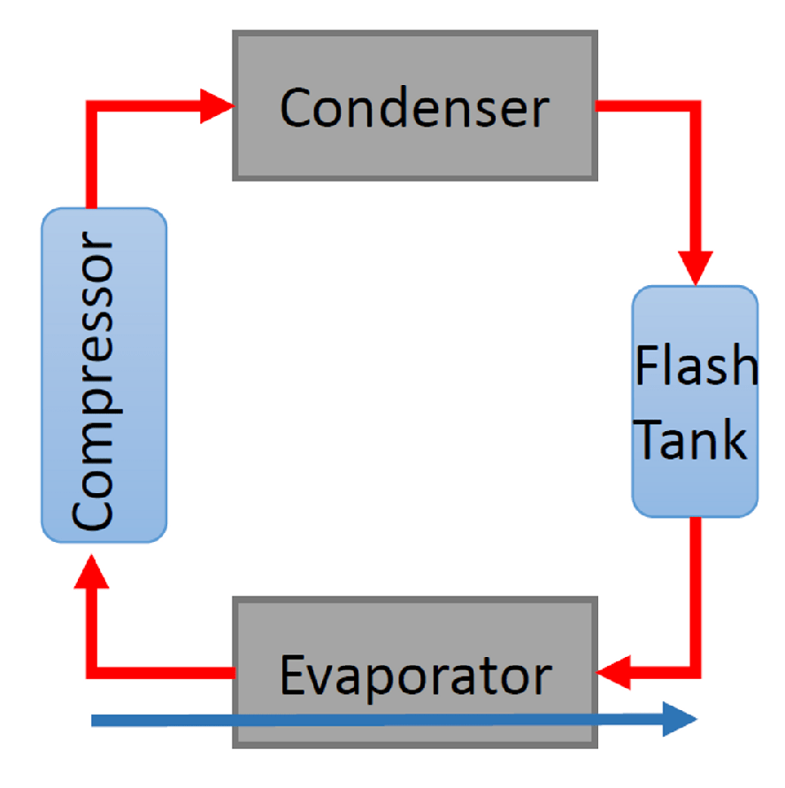
The CU is a vapor cycle refrigeration unit consisting of a compressor, a condenser, an evaporator and a flash tank (see Figure 4). After many days of operations, the CU becomes clogged with burned oil, moisture, and sludge from the compressor. This accelerates the compressor wear. Long-term exposure to these conditions negatively affects the health of the CU, which, in time, leads to failure [41].

3.1. Health Indicator For CUs

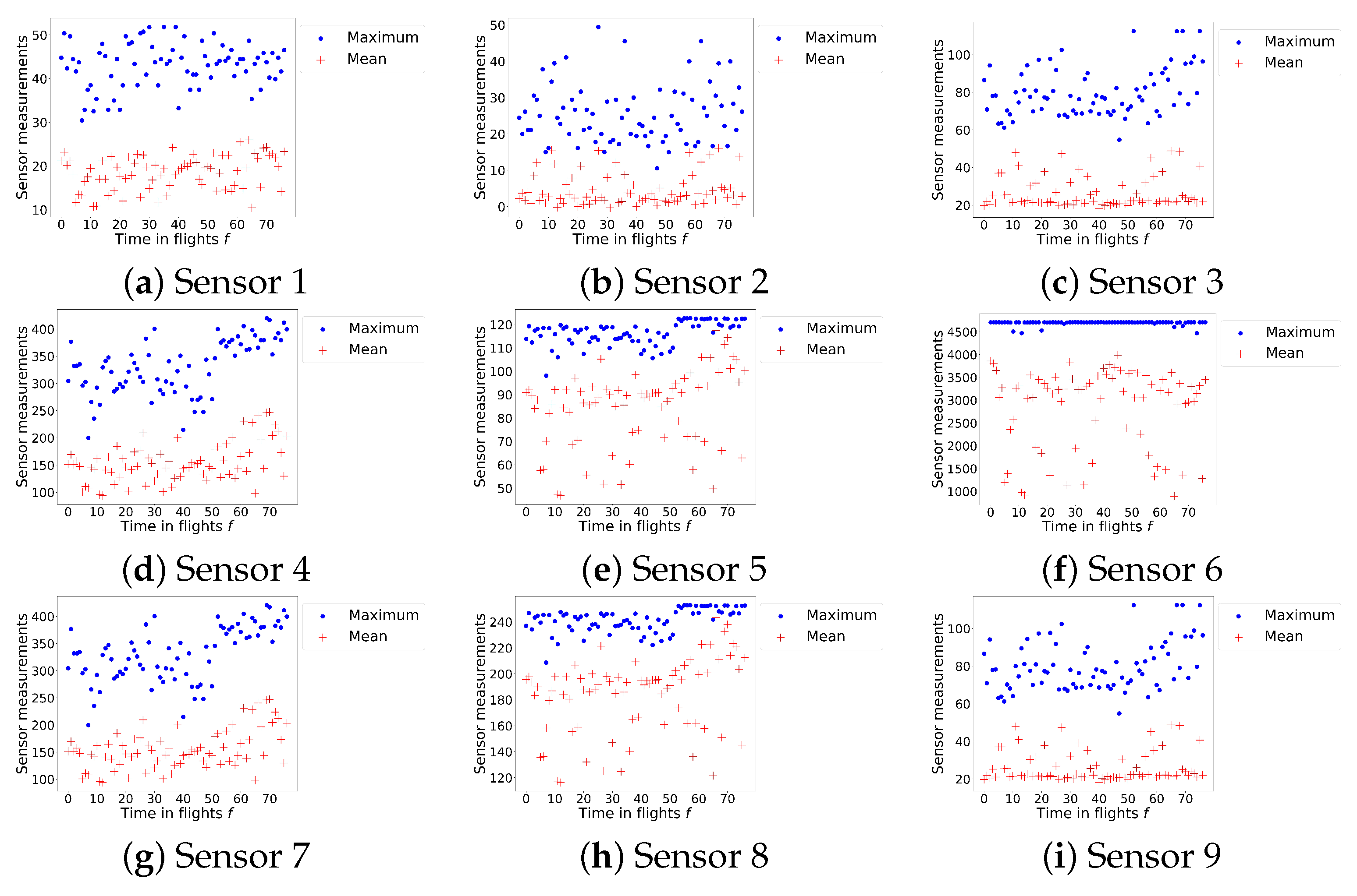
For each CU, run-to failure measurements were considered. These measurements were available after some initial usage of the component. The run-to-failure data series consists of sequences of 50 flights (short series) up to 390 flights (long series). For each CU, there were nine sensors $S=\{1,2,\dots ,9\}$, each generating a measurement every 10 s during each flight. For the purpose of our analysis, the data sets are anonymized, and thus it is unknown the type of measurement each sensor generates. We observed, in the sensor data, an increasing trend in the mean and maximum sensor measurements toward failure. As an example, Figure 5 shows the mean and maximum sensor measurements per day until the moment of failure for one CU and for each of the nine available sensors.

Let $y_{f,b}^{i,s}$ denote the $b^{th}$ measurement during flight f for CU i generated by sensor s. We first normalize the sensor measurements as follows:

$${\widehat{y}}_{f,b}^{i,s}=\frac{y_{f,b}^{i,s}-{\min }_s}{{\displaystyle {\max }_s-\underset{b\in 1,\dots ,B_f^i}{max}\left(y_{f,b}^{i,s}\right)}},s\in \{1,2,\dots ,9\},$$

(18)

with the ${\min }_s$ and ${\max }_s$ the available minimum and maximum measurements generated by sensor s, respectively, and $B_f^i$ as the total number of measurements recorded during flight f of CU i.

With these normalized sensor measurements, we considered several health indicators, as described in [2,42]. We constructed each health-indicator for the measurements of each sensor and calculated, for each sensor, the correlation coefficient (trendability) between the health indicator and the time to failure for the last 50 flights before failure (length of the shortest serie).

Table 1. Overview of the considered health indicators. For each sensor, the correlation coefficient between the health indicator and the time to failure is given. The highest absolute correlation coefficient is given in bold.

Health-Indicator	Sensors
	1	2	3	4	5	6	7	8	9
${\mathrm{RMS}}_f=\sqrt{\frac{1}{B_f^i}{\sum }_{b=1}^{B_f^i}{\left({\widehat{y}}_{f,b}^{i,s}\right)}^2}$	−0.06	0.12	0.27	0.45	0.46	−0.13	0.44	0.47	0.26
$\Delta {\mathrm{RMS}}_f={\mathrm{RMS}}_f-{\mathrm{RMS}}_{f-1}$	0.02	0.01	0.02	0.02	0.01	−0.01	0.02	0.01	0.02
${\mathrm{Peak}-\mathrm{to}-\mathrm{peak}}_f=$
${\displaystyle \underset{b\in 1,\dots ,B_f^i}{max}\left({\widehat{y}}_{f,b}^{i,s}\right)-\underset{b\in 1,\dots ,B_f^i}{min}\left({\widehat{y}}_{f,b}^{i,s}\right)}$	−0.08	0.11	0.24	0.43	0.38	−0.16	0.44	0.38	0.25
$\mathrm{Crest}{\mathrm{Factor}}_f=\frac{{\displaystyle \underset{b\in 1,\dots ,B_f^i}{max}\left({\widehat{y}}_{f,b}^{i,s}\right)}}{{\mathrm{RMS}}_f}$	−0.05	0.06	0.08	−0.02	−0.06	0.08	−0.02	−0.06	0.13
${\mathrm{Kurtosis}}_f$	−0.03	$-\mathbf{0}.\mathbf{11}$	0.05	$-\mathbf{0}.\mathbf{11}$	0.05	0.10	$-\mathbf{0}.\mathbf{11}$	0.05	0.05
${\mathrm{Skewness}}_f$	$-\mathbf{0}.\mathbf{13}$	0.09	0.05	−0.11	−0.03	−0.00	−0.11	−0.03	0.05

provides an overview of the considered health-indicators and the corresponding correlation coefficients. An extensive description of the health indicators can be found in [42].

The highest correlation coefficients were obtained for the Root Mean Square (RMS) health indicator. We, thus, constructed a health indicator based on the RMS of the measurements [10,42,43]. A health indicator based on the RMS of measurements was often employed in the literature [2,42], for example for the health monitoring of gearboxes [44], turbine-cutting tools [43], and rolling element bearings [45]. The RMS of sensor s of CU i during flight f is:

$$RM{S}_f^{i,s}=\sqrt{\frac{1}{B_f^i}\sum _{b=1}^{B_f^i}{\left({\widehat{y}}_{f,b}^{i,s}\right)}^2}.$$

(19)

A health indicator ${\mathcal{I}}_f^i$ for CU i during flight f was obtained as the moving average of the maximum RMS obtained by the sensors $s\in S^{\prime }$, as follows:

$${\mathcal{I}}_f^i=\frac{1}{N}\left(\sum _{l=f-N}^f\left({\displaystyle \underset{s\in S^{\prime }}{max}RM{S}_l^{i,s}}\right)\right),$$

(20)

where $N=10$ and where $S^{\prime }\subseteq S$ is the set of sensors for which the moving average of the RMS of the measurements obtained in the last 50 flights before failure has a correlation coefficient with the time of failure of at least 0.70. We, therefore, included sensors 4, 5, 7, and 8 in the health-indicator. This final health indicator emphasizes the increase in the mean and the maximum measurements toward failure, which we observe in Figure 5.

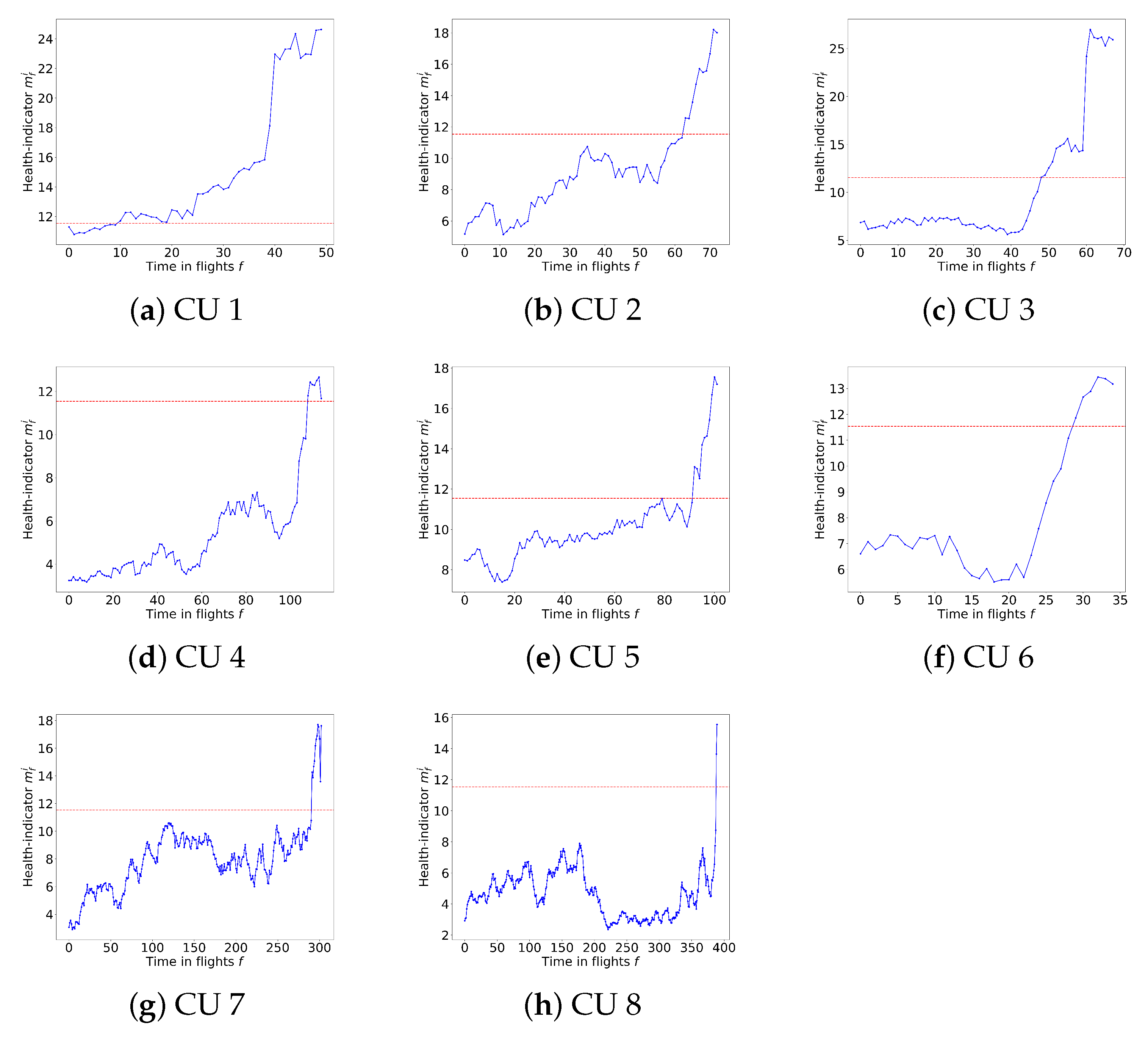
Figure 6 shows the health indicator and the alarm threshold $T^{\mathrm{alarm}}$ when considering the run-to-failure data of the eight CUs. For the alarm threshold, we assume $k=2$ (see Equation (3)), obtaining a threshold of $T^{\mathrm{alarm}}=11.54$. When analyzing all CUs, the alarm threshold is reached between 2 to 40 flights before the actual failure time.

Figure 6 also shows that the degradation trends toward failure, which differed across components. The failure thresholds differed among the eight components. As such, in the next section, we cluster the series of health indicators to identify the main degradation models and the corresponding failure thresholds.

3.2. Clustering the Health Indicators and Determining Clustering-Specific Degradation Models

We performed dynamic time-warping (see Section 2.2, Step 2) to cluster the $n=8$ time series of health indicators and to identify cluster-specific degradation models for the CUs. For this, we used the run-to-failure data of the eight CUs, starting $m=10$ flights before the CU reached the alarm threshold until failure time.

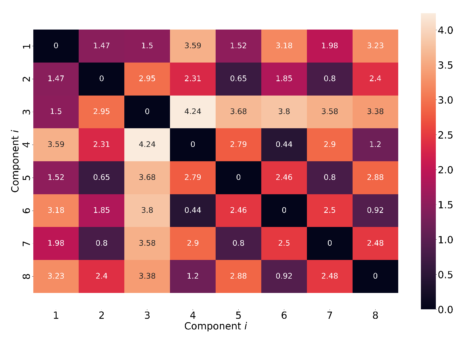
Figure 7 shows the minimum distance $W({\mathcal{I}}^i,{\mathcal{I}}^j)$, $i,j\in \{1,2,\dots ,8\}$, between the series of health indicators of the eight CUs, normalized with the maximum length of the series ${\mathcal{I}}^i$ and ${\mathcal{I}}^j)$. Here, the minimum distances $W({\mathcal{I}}^i,{\mathcal{I}}^j)$ between the degradation of any two components varies from 0.44 (high similarity between the degradation trends) to 4.24 (large dissimilarities between the degradation trends).

Using $W({\mathcal{I}}^i,{\mathcal{I}}^j),i,j\in \{1,2,\dots ,8\}$, between the eight series of health indicators, we constructed the graph $G(V,E)$, with $\left|V\right|=8$. Here, a node $v^i\in V$ in the graph corresponds to the series of health indicators for component $i,i\in \{1,2,\dots ,8\}$. For each CU i, and a given $\delta$, an edge was constructed between those $\delta$ nodes (CUs) that have the smallest distance to node $v^i$ (CU i). For example, if $\delta =2$ and we consider CU $i=4$, an edge was constructed between node $v^4$ and node $v^6$ and between node $v^4$ and $v^8$, since the distances between node $v^4$ and nodes $v^6$ and $v^8$ are the smallest (see Figure 7).

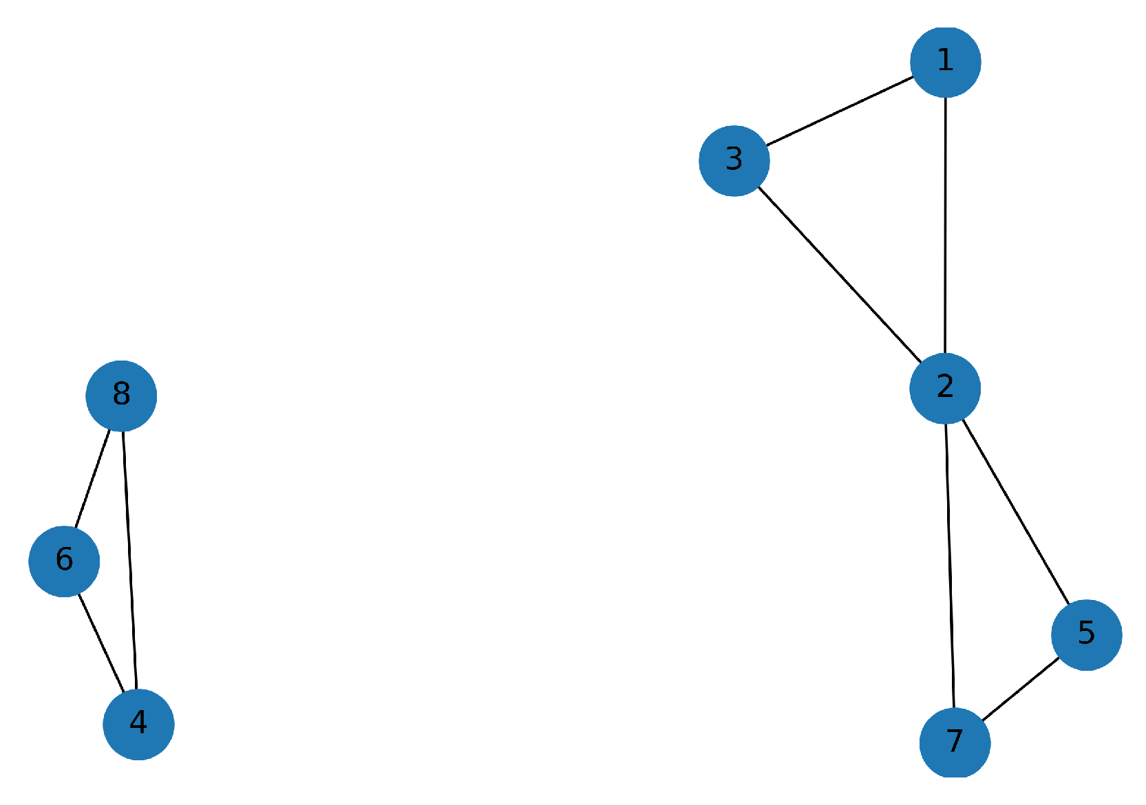
In Figure 8, we set $\delta =1$. This results in two clusters of CUs: $\{4,6,8\}$, and CU $\{1,2,3,5,7\}$. The health indicator in Figure 6 shows that the CUs 4, 6, and 8 failed soon after the health indicator reached the alarm threshold—when the health indicator reached a value of approximately 15. The degradation trend around failure showed a monotonic increase. In contrast, CUs 1,2,3,4,5, and 7 failed when the health indicator reached a value of 20. Furthermore, the degradation of these CUs often accelerated toward failure.

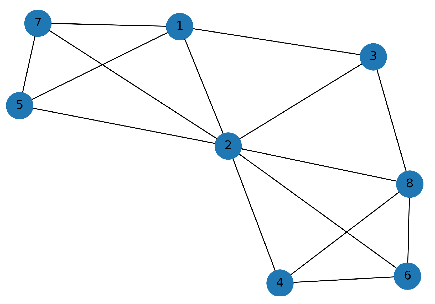
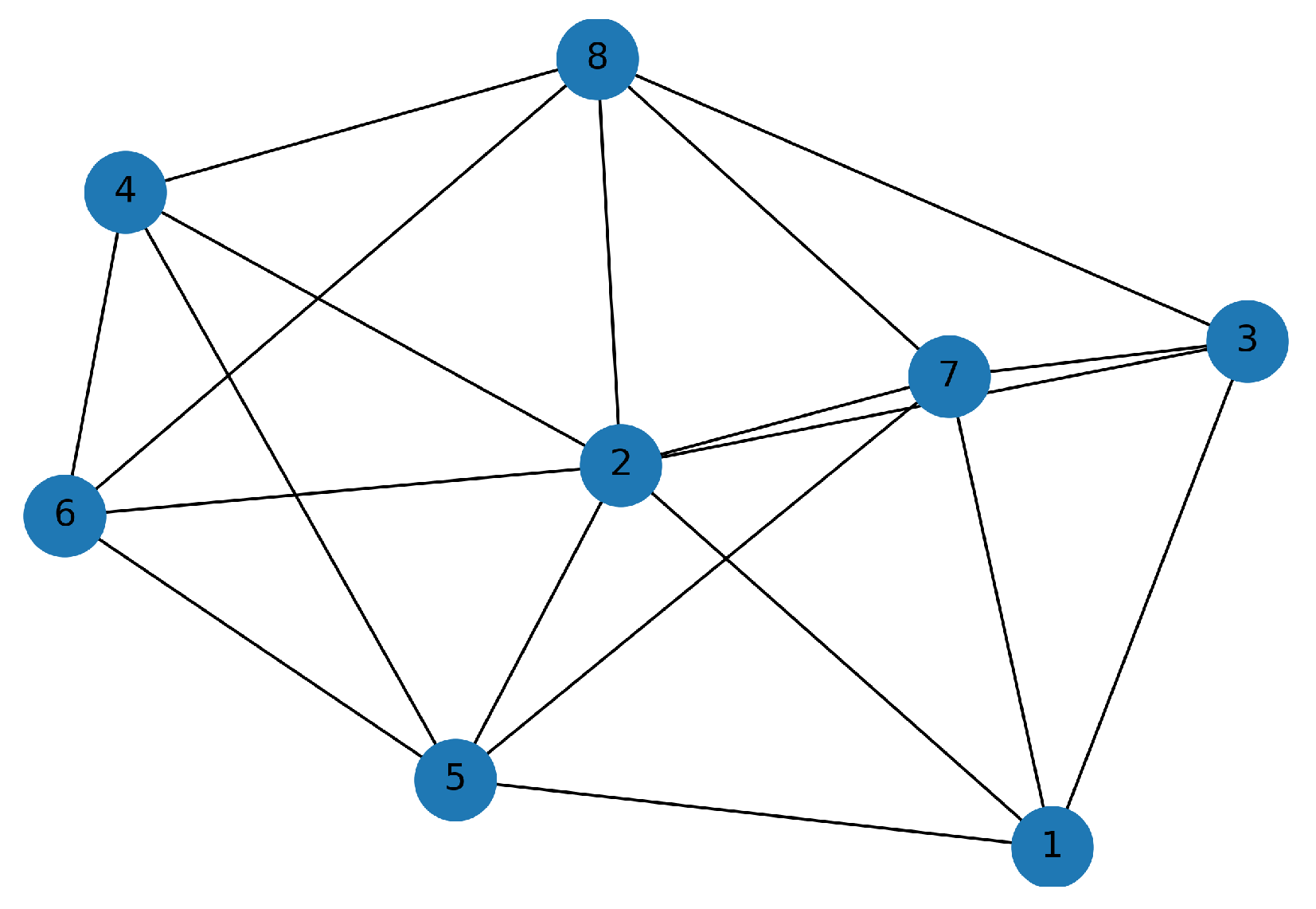
For $\delta =2$ (see Figure 9), the same two clusters $\{4,6,8\}$ and $\{1,2,3,5,7\}$ are maintained. The CUs in Figure 9 are now connected by multiple edges. For $\delta =3$ (see Figure 10), only one large cluster emerges. Here, the CUs in cluster $\{4,6,8\}$ and cluster $\{1,2,3,5,7\}$ are still grouped together (see Figure 8), and connected to each other through CU 2 and 3. Finally, for $\delta =4$ (see Figure 11), all CUs formed one large cluster with several edges between clusters $\{4,6,8\}$ and $\{1,2,3,5,7\}$. Following the clustering for different $\delta$, we define the following two clusters:

$$\begin{array}{cc}\hfill \mathrm{Cluster}1& =\{4,6,8\}\hfill \end{array}$$

(21)

$$\begin{array}{cc}\hfill \mathrm{Cluster}2& =\{1,2,3,5,7\}.\hfill \end{array}$$

(22)

For the two clusters in Equations (21) and (22), we now define the following cluster-specific degradation models.

3.3. Cluster 1—Linear Degradation Model

The health indicators of CUs 4, 6, and 8 in Cluster 1 are given in Figure 6d,f,h. All these CUs fail when their health indicator reached a value of approximately 15. Thus, we consider a failure threshold $D=15$ for Cluster 1. Once the health indicator of the CUs in Cluster 1 reaches the alarm threshold $T^{\mathrm{alarm}}$, the indicator had a sharply, but monotonic increasing, trend toward failure. We, thus, consider the following linear degradation model for the CUs in Cluster 1 [8]:

$$X_t^i={\alpha }^i+{\beta }^{i}t+{\omega }^i$$

(23)

where $X_t^i$ is the degradation of component i at time t, ${\alpha }^i$ is the initial degradation, ${\beta }^i$ is a model parameter, and ${\omega }^i$ is the noise in the degradation process. As in [30], we ignore the process noise because it is handled through the uncertainty in the model parameters and in the measurements [46]. Linear degradation models are often considered for prognostics [24], for example for milling machines [25], batteries [26], aircraft engines [27], and engine bleed valves [28].

Following the degradation model in Equation (23), we consider the derivative:

$$d{X}_t^i={\beta }^{i}dt.$$

(24)

Rewriting the above equation in the form of Equations (10) and (1) with $dt=1$ flight, we obtain:

$$\begin{array}{cc}\hfill X_f^i& =X_{f-1}^i+{\beta }_f^i\hfill \end{array}$$

(25)

$$\begin{array}{cc}\hfill {\mathcal{I}}_f^i& =X_f^i+{\nu }_f^i\hfill \end{array}$$

(26)

where ${\nu }_f^i\sim N(0,{\sigma }_{{\nu }_f^i})$ is the measurement noise at flight f. The distributions of the model parameters are initialized as ${\beta }_0^i\sim U(0.01,1)$ and ${\sigma }_{{\nu }_0^i}\sim U(1,2)$.

The parameter distributions are initialized such that sample impoverishment, the degeneracy problem and non-convergence of the particle filtering algorithm are avoided [46].

3.4. Cluster 2—Exponential Degradation Model

The health indicators of CUs 1,2,3,5, and 7 in Cluster 2 are given in Figure 6. All these CUs failed when their health indicator reached a value of approximately 20. Thus, we consider a failure threshold $D=20$ for Cluster 2.

Moreover, the increments of the health indicator steadily increased toward failure for these CUs. We, thus, consider the following exponential degradation model for the CUs in Cluster 2:

$$X_t^i={\alpha }^i+exp\left({\beta }^{i}t\right)+{\omega }^i$$

(27)

where $X_t^i$ is the degradation of component i at time t, ${\alpha }^i$ is the initial degradation, ${\beta }^i$ is a model parameter, and ${\omega }^i$ is the noise in the degradation process. As before, we ignore the process noise [30]. Exponential degradation models have been considered in many prognostic studies [24], for bearings [29,31], batteries [30,32], and railway turnout systems [33].

Taking the logarithm of Equation (27):

$$S_t^i=ln(X_t^i-{\alpha }_i)={\beta }^{i}t.$$

(28)

As in [8], we assume that ${\alpha }_i=0$. Following the degradation model in Equation (28), we consider the derivative:

$$d{S}_t^i={\beta }^{i}dt.$$

(29)

Rewriting the above equation in the form of Equations (10) and (1) with $dt=1$ flight, we obtain:

$$\begin{array}{cc}\hfill S_f^i& =S_{f-1}^i+{\beta }_f^i\hfill \end{array}$$

(30)

$$\begin{array}{cc}\hfill {\mathcal{I}}_f^i& =X_f^i+{\nu }_f^i,\hfill \end{array}$$

(31)

where ${\nu }_f^i\sim N(0,{\sigma }_{{\nu }_f^i})$ is the measurement noise at flight f. The distributions of the model parameters are initialized as ${\beta }_0^i\sim U(0.01,0.1)$ and ${\sigma }_{{\nu }_0^i}\sim U(1,2)$. The parameter distributions are initialized such that sample impoverishment, the degeneracy problem, and the non-convergence of the particle filtering algorithm are avoided [46].

Lastly, with the degradation models introduced above, we apply the particle filtering algorithm (see Section 2, Step 4) to estimate the RUL of the CUs.

3.5. Rul Estimation Results

In this section, we estimate the RUL of the eight CUs using leave-one-out cross validation as follows. We select one CU $i\in \{1,2,\dots ,8\}$. We consider the (partial) health indicator of this CU i up to the moment of generating a RUL prediction. We determine the minimum distance between this (partial) health indicator and the (partial) health indicators of the CUs in Cluster 1 and Cluster 2 (see Equations (21) and (22)), which do not include CU i. We assign CU i to that cluster for which the average distance between the cluster and CU i is the minimum (see Step 3, Section 2). Then, CU i assumes the degradation model and the failure threshold of this cluster. Lastly, we estimate the RUL of CU i using particle filtering with 10,000 particles.

Table 2. RUL prediction (in flights) for the CUs. The RUL is estimated once the CU becomes alerted and 10 flights before failure.

	RUL Prediction as Soon as CU Is Diagnosed as Unhealthy			RUL Prediction 10 Flights before Failure (RUL = 10)
CU $\mathit{i}$	Actual RUL at ${\mathit{f}}^{\mathit{i},\mathrm{alarm}}$	Assigned Cluster	Estimated RUL	Assigned Cluster	Estimated RUL
1	40	2 (Exp.)	36	2 (Exp.)	2
3	20	1 (Lin.)	10	2 (Exp.)	7
7	12	2 (Exp.)	11	2 (Exp.)	6
2	10	2 (Exp.)	9	2 (Exp.)	9
5	10	2 (Exp.)	8	2 (Exp.)	8
4	7	1 (Lin.)	10	-	-
6	6	1 (Lin.)	7	-	-
8	2	1 (Lin.)	1	-	-
RMSE			4.04		4.34

shows for each CU the cluster it is assigned to as soon as $T^{\mathrm{alarm}}$ is reached, i.e., the CU is diagnosed as unhealthy, and there is a corresponding RUL prediction. CU 1 was diagnosed as unhealthy, and an alarm was triggered at an early stage at 40 flights before the actual failure time. CUs 2, 3, 4, 5, 6, and 7 were diagnosed as unhealthy up to six flights before the actual failure. For CU 8, an alarm was triggered only two flights before the actual failure.

CUs 1, 2, 5, and 7 were assigned to Cluster 2, which assumed an exponential degradation model, whereas CUs 3, 4, 6, and 8 were assigned to Cluster 1, which assumed a linear degradation model. Only CU 3 was assigned to a different cluster (namely cluster 1) than in the offline clustering, which led to underestimation of the RUL. These results show that, even when considering clustering with partial health indicators, i.e., up to the moment when a prediction is made, our approach can well identify the underlying linear or exponential degradation trend and the corresponding failure threshold.

Table 2 shows the RUL estimates 10 flights before the time of failure. CUs 4, 6, and 8 failed within less than 10 flights as soon as they were diagnosed as unhealthy, thus, no RUL predictions are made in this case. CUs 1, 2, 3, 5, and 7 were all assigned to the same exponential cluster as in the offline clustering.

Table 2 also shows that the RUL of the CUs was well estimated as soon as these CUs were diagnosed as unhealthy. The Root Mean Square Error (RMSE) was low as well. The fact that we were able to select appropriate degradation models and failure thresholds based on cluster-specific trends contributes to the accuracy of the RUL predictions.

4. Conclusions

We proposed an online, model-based RUL estimation approach for aircraft components using a clustering of component degradation trends. Using clustering, we determined cluster-specific degradation models and failure thresholds. Together with a particle filtering algorithm, these degradation models were used to estimate the RUL of multiple, same-type aircraft components.

As an illustration, we considered several aircraft Cooling Units for which sensor measurements were recorded during the operation of the aircraft. The results show that our proposed methodology was able to identify the degradation models of components and estimate their RUL. From a practical point of view, our RUL estimation results have the potential to support aircraft maintenance stakeholders with maintenance task scheduling.

For future work, we plan to extend our methodology for other aircraft components. At the same time, we plan to propose maintenance task scheduling algorithms to evaluate the impact of prognostic-driven maintenance on the maintenance costs and aircraft availability.