Theory of Contrail Formation for Fuel Cells

Abstract

The theory of contrail formation for fuel cells is derived. It is a variant of the well-known Schmidt-Appleman theory. The contrail factor or G-factor for fuel cells is much larger than for jet engines, such that condensation of the exhaust water vapour can happen even at the Earth’s surface in sufficiently cold (a few degrees above zero) weather. Contrail formation from fuel cells will occur frequently in the lower troposphere and is unavoidable below moderate temperature limits, in the upper troposphere and in the stratosphere. Despite the high frequency of contrail formation from fuel cells, their climate impact is lower than that of contrails from jet engines. Most fuel cell contrails will be short and those persistent ones will be optically thinner and have on average a shorter lifetime than traditional persistent contrails. From a climate point of view, the introduction of fuel cells into aviation can be recommended.

1. Introduction

The thermodynamic theory of contrail formation has been formulated in the last century for turboprops and jet engines by Schmidt [1] and Appleman [2]; the theory is thus named after these researchers. It is founded on the principle that the mixing of two airmasses with different temperature and humidity can lead to a supersaturated state, which induces condensation. A common weather phenomenon that is based on this principle is mixing-fog. A modern derivation of the theory has been presented by Schumann [3].

Condensation of water droplets in the atmosphere usually needs condensation nuclei, tiny aerosol particles on which the water vapour can attach and form droplets. Such nuclei are always present, but for traditional engines the burning of kerosene is a more prolific source of particles, viz. soot, which is emitted at a much higher number (about ${10}^{15}$ particles per kg of kerosene) than the number density of natural aerosol [4]. However, contrails form using emitted volatile aerosol [5] or ambient aerosol [6] as condensation nuclei if no soot is present in the exhaust, for example, if burning liquid hydrogen. The presence of condensation nuclei is not a constraint for contrail formation and thus not part of the theory.

Contrails contribute considerably to the climate impact of aviation [7]. Only persistent contrails are climate-effective, and these form in ice-supersaturated air masses, so-called ice-supersaturated regions, ISSRs [8]. Ideas for the avoidance of persistent contrails are discussed since many years [9,10,11]. The suggested measures divide into operational and technical measures. Operational contrail avoidance implies avoiding flying in ISSRs, which needs a good weather forecast for flight planning, which still needs considerable improvement [12]. Technical possibilities involving a deterioration of the overall propulsion efficiency, for example, via variable guide vanes [13], are certainly not the best option. Use of alternative fuels with lower soot emission or no soot at all, although not avoiding contrails completely, may be better [14,15]. For all such measures contrail formation can be computed with the traditional form of the Schmidt-Appleman criterion; only some characteristic values like the emission index of water vapour, EI${}_{{\mathrm{H}}_2\mathrm{O}}$, the specific energy content of the fuel, Q, and the overall propulsion efficiency, $\eta$, need to be adapted. The Schmidt-Appleman criterion leads to a so-called contrail factor or G-factor, which is the starting point for further considerations. Its traditional formula is:

$$G=\frac{c_p{p}_a}{\epsilon }\frac{{\mathrm{EI}}_{{\mathrm{H}}_2\mathrm{O}}}{(1-\eta )Q}.$$

(1)

The atmospheric properties are represented in this equation by the ambient pressure, $p_a$. $c_p$ is the heat capacity of air and $\epsilon =0.622$ is the ratio of the molar masses of water and air. The meaning of the G-factor will be explained below.

Future propulsion concepts like multi-fuel engines [16] or hybrid electric/gas-turbine combinations [17] need modifications to the form of the Schmidt-Appleman formula. For instance, if the hybrid propulsion is based on electric energy provided by batteries, the water emission of this part of the propulsion is zero. This has to be accounted for in a modification of the Schmidt-Appleman formula. Batteries are heavy and are thus merely a possibility for small aircraft with short range. For medium range aircraft the electric energy must be produced by a generator which is driven by a gas turbine or a fuel cell. These engines emit water vapour and again the Schmidt-Appleman criterion needs to be modified.

In the present paper, I derive the Schmidt-Appleman criterion for fuel cells in aviation. The theory is developed in Section 2 and the consequences for contrail formation in the atmosphere are shown. Section 3 provides a discussion of the climatic implications and conclusions are drawn in the final Section 4.

2. Theory

2.1. The Schmidt-Appleman Criterion for Fuel Cells

The physical process behind the formation of contrails is the mixing of two airmasses, one warm and moist (the exhaust gases), the other cold and drier (ambient air). This mixing may lead to a supersaturated state and then droplets can form, which may freeze if they get sufficiently cold. An aircraft exhaust plume mixes isobarically with the ambient air, such that its state-point in a temperature vs. water vapour partial pressure diagram follows a straight line, see, for instance, Figure 3 of [3]. The condition for condensation of droplets, supersaturation with respect to liquid supercooled water, is met if the mixing line crosses the curve of saturation pressure (saturation with respect to liquid supercooled water). In such a case, a contrail is formed.

The mixing trajectory has the slope

$$G=\frac{e_p-e_a}{T_p-T_a},$$

(2)

where the indices “p” and “a” mean “plume” and “ambient”. The denumerator is related to mass conservation of water, where $e_x$ is the partial pressure of water vapour. The denominator expresses energy conservation, and $T_x$ are the static temperatures.

Engineers may skip the rest of this section and jump directly to Section 2.5, because the calculations that follow are in a certain sense academic; they consider the unaltered exhaust from a fuel cell. This leads to a form of the G-factor that is similar to its traditional form and it yields physical insight. However, technical manipulations of the exhaust, like heat exchanger and condenser for water vapour differ from case to case; they cannot be covered by a common formula of the traditional form. In this case, an engineer can still use the basic definition of G above if only the parameters at exhaust exit ($e_p,T_p$) and their atmospheric counterparts are known. For the unmodified exhaust gases these parameters can be computed with basic physical considerations, which will be done in the following.

Starting with mass conservation, the flows of matter into and out of the fuel cell (FC) are considered in terms of molar fluxes (units mole per second, mole s${}^{-1}$). The fed-in air and hydrogen fuel can be considered ideal gases, such that pressure ratios equal the number or molar ratios. Let the input rate of the FC consist of ${\dot{\nu }}_{{\mathrm{H}}_2}$ moles s${}^{-1}$ of H${}_2$ and ${\dot{\nu }}_{\mathrm{air}}$ moles s${}^{-1}$ of air. The air consists mainly of nitrogen, N${}_2$, oxygen, O${}_2$, with a molar fraction $X_{{\mathrm{O}}_2}\approx 0.2$, and ambient water vapour with a molar fraction $e_a/p_a$. Hydrogen and oxygen react to water vapour in the following reaction:

$${\mathrm{H}}_2+{}^1{/}_2{\mathrm{O}}_2\to {\mathrm{H}}_2\mathrm{O},$$

(3)

which yields one mole of water per one mole of hydrogen and half a mole of oxygen. Thus the output rate at the FC exit in moles s${}^{-1}$ is lower than that at the input, since $1{}^1{/}_2$ moles are converted into one mole in the reaction.

If all hydrogen molecules are consumed in the reaction, the reaction rate equals the rate at which H${}_2$ is fed in, ${\dot{\nu }}_{{\mathrm{H}}_2}$. The rate at which O${}_2$ from the ambient air is consumed is half as large, ${}^1{/}_2{\dot{\nu }}_{{\mathrm{H}}_2}$, and the rate at which water molecules are added to the exhaust gases equals the rate at which H${}_2$ is fed in, ${\dot{\nu }}_{{\mathrm{H}}_2\mathrm{O}}={\dot{\nu }}_{{\mathrm{H}}_2}$. The FC output thus has a total gas flow of ${\dot{\nu }}_{\mathrm{air}}-{}^1{/}_2{\dot{\nu }}_{{\mathrm{H}}_2}+{\dot{\nu }}_{{\mathrm{H}}_2\mathrm{O}}={\dot{\nu }}_{\mathrm{air}}+{}^1{/}_2{\dot{\nu }}_{{\mathrm{H}}_2\mathrm{O}}$ moles s${}^{-1}$, since the input flux of hydrogen equals the output flux of water vapour produced in the reaction (3). The water vapour fraction of the output consists of the produced water plus the water from the input air, which flows in and out with the rate $(e_a/p_a){\dot{\nu }}_{\mathrm{air}}$. The molar ratio of water vapour at the FC exit is thus

$$\frac{e_p}{p_a}=\frac{{\dot{\nu }}_{{\mathrm{H}}_2\mathrm{O}}+(e_a/p_a){\dot{\nu }}_{\mathrm{air}}}{{}^1{/}_2{\dot{\nu }}_{{\mathrm{H}}_2\mathrm{O}}+{\dot{\nu }}_{\mathrm{air}}},$$

(4)

where the assumption is made that the exhaust gas obtains immediately the ambient pressure (which is a reasonable assumption since any pressure contrasts are relaxed at the speed of sound; see the chapter on elastic waves in any physics textbook). After a short calculation, one finds

$$e_p-e_a=p_a\frac{{\dot{\nu }}_{{\mathrm{H}}_2\mathrm{O}}[1-{}^1{/}_2(e_a/p_a)]}{{}^1{/}_2{\dot{\nu }}_{{\mathrm{H}}_2\mathrm{O}}+{\dot{\nu }}_{\mathrm{air}}}.$$

(5)

Since $e_a/p_a\ll 1$ one may neglect this contribution to find the desired expression for $e_p-e_a$ as:

$$e_p-e_a=p_a\frac{{\dot{\nu }}_{{\mathrm{H}}_2\mathrm{O}}}{{}^1{/}_2{\dot{\nu }}_{{\mathrm{H}}_2\mathrm{O}}+{\dot{\nu }}_{\mathrm{air}}}.$$

(6)

For the consideration of energy conservation, it will be useful to begin with a few thermodynamic considerations of the involved quantities. Assuming that the FC operates such that the water is produced as steam, not as liquid water, implies that one needs to choose the so-called lower heating values of the thermodynamic variables. At standard conditions (i.e., pressure 1 bar or ${10}^5$ Pa and temperature 25 ${}^{\circ }$C or $298.15$ K), the formation enthalpy of water vapour from its constituent elements is $\Delta h^0=-241.82$ kJ mol${}^{-1}$ and the corresponding free enthalpy (or Gibbs free enthalpy) is $\Delta g^0=-228.57$ kJ mol${}^{-1}$ (Table A 1.1 of [18]). The free enthalpy (instead of the free energy) is relevant here as the reaction occurs at constant pressure and temperature in the FC. It is the maximum non-expansive work, that is, the maximum electric work, the FC can perform. In the reaction (3) the entropy of the reactants is higher than the entropy of the product by $|\Delta s^0|=44.4$ J$(\pm )$ K${}^{-1}$ at standard conditions. Thus it is necessary that a part of the reaction enthalpy is used to heat the exhaust gases in order to guarantee that the overall entropy change is not negative. This “entropy tax” is expressed by the difference between $\Delta h^0$ and $\Delta g^0$. It is heat that increases the temperature of the exhaust gases.

Generally, an FC will work under conditions that are different from the standard conditions and the thermodynamic quantities $\Delta h$ and $\Delta g$ will differ from $\Delta h^0$ and $\Delta g^0$. The differences are however small (see for instance [18], Chapter 2.7, [19], Chapter 2.4, or [20], Chapter 4.4.2). Thus only small errors incur in numerical calculations if one uses the enthalpy and free enthalpy in standard conditions. In order to present the results for general conditions, $\Delta h$ and $\Delta g$ (without the superscript 0) are used in the following derivations.

The fuel cell is characterized by its electromotive force $\mathcal{E}$, which depends on the free enthalpy of the reaction (3):

$$\mathcal{E}=-\frac{\Delta g}{2F},$$

(7)

where Faraday’s constant F is the number of negative elementary charges per mole of electrons, expressed in C mol${}^{-1}$: $F=96,485$ C mol${}^{-1}$. F is multiplied by 2 since 2 electrons flow from the anode to the cathode [18,19,20]. The electromotive force of the hydrogen fuel cell is $\mathcal{E}=1.19$ V (if the water is released in gaseous state). The electromotive force is an ideal voltage of the cell which requires an infinite resistance between the electrodes, thus zero current. Once the cell operates and produces work, its current is given by the rate of the reaction

$$I={\dot{\nu }}_{{\mathrm{H}}_2\mathrm{O}}·2F,$$

(8)

its actual voltage U is less than $\mathcal{E}$, typically in the range $0.5$ to 1 V (see Figure 4.3 of [20]), and thus the electric power that can be used to drive an engine is $UI$. The remaining power $(\mathcal{E}-U)I$ contributes to heat the exhaust gases, which adds to the “entropy tax”, ${\dot{\nu }}_{{\mathrm{H}}_2\mathrm{O}}(\Delta h-\Delta g)$ mentioned above.

The energy balance of the working FC is thus

$$-{\dot{\nu }}_{{\mathrm{H}}_2\mathrm{O}}\Delta h=UI+(\mathcal{E}-U)I-{\dot{\nu }}_{{\mathrm{H}}_2\mathrm{O}}(\Delta h-\Delta g).$$

(9)

That is, the reaction enthalpy of the oxyhydrogen reaction is split into electric work and heating of the exhaust due to a lower than ideal voltage of the FC and due to the entropy tax.

It will turn out useful to introduce two efficiencies, a basic efficiency

$${\eta }_0=\Delta g/\Delta h$$

(10)

and an electric efficiency

$${\eta }_E=U/\mathcal{E}.$$

(11)

With these efficiencies the energy balance reads

$$-{\dot{\nu }}_{{\mathrm{H}}_2\mathrm{O}}\Delta h={\eta }_E\mathcal{E}I-(1-{\eta }_E{\eta }_0){\dot{\nu }}_{{\mathrm{H}}_2\mathrm{O}}\Delta h.$$

(12)

The power that heats the exhaust is thus $(1-{\eta }_E{\eta }_0){\dot{\nu }}_{{\mathrm{H}}_2\mathrm{O}}|\Delta h|$. The product ${\eta }_E{\eta }_0$ can be conceived to be the efficiency of the fuel cell.

The heat capacity of the input air is $c_{p,\mathrm{air}}=29.1$ J mol${}^{-1}$ K${}^{-1}$ and that of gaseous water is $c_{p,{\mathrm{H}}_2\mathrm{O}}=33.6$ J mol${}^{-1}$ K${}^{-1}$ [18]. The waste heat and entropy tax warms the air as follows:

$$(1-{\eta }_E{\eta }_0){\dot{\nu }}_{{\mathrm{H}}_2\mathrm{O}}|\Delta h|=c_{p,{\mathrm{H}}_2\mathrm{O}}(T_p-T_a){\dot{\nu }}_{{\mathrm{H}}_2\mathrm{O}}+c_{p,\mathrm{air}}(T_p-T_a)({\dot{\nu }}_{\mathrm{air}}-{}^1{/}_2{\dot{\nu }}_{{\mathrm{H}}_2\mathrm{O}}).$$

(13)

Solving the energy balance for $T_p-T_a$ yields

$$T_p-T_a=\frac{(1-{\eta }_E{\eta }_0)|\Delta h|{\dot{\nu }}_{{\mathrm{H}}_2\mathrm{O}}}{c_{p,{\mathrm{H}}_2\mathrm{O}}{\dot{\nu }}_{{\mathrm{H}}_2\mathrm{O}}+c_{p,\mathrm{air}}({\dot{\nu }}_{\mathrm{air}}-{}^1{/}_2{\dot{\nu }}_{{\mathrm{H}}_2\mathrm{O}})}.$$

(14)

In principle, the ingredients to calculate $G_{\mathrm{FC}}$ are now at hand, but the presence of different heat capacities would lead to an unwieldy expression. One can achieve a more concise expression defining a mean heat capacity of the exhaust gases as follows:

$$\overline{c_p}=\frac{c_{p,{\mathrm{H}}_2\mathrm{O}}{\dot{\nu }}_{{\mathrm{H}}_2\mathrm{O}}+c_{p,\mathrm{air}}({\dot{\nu }}_{\mathrm{air}}-{}^1{/}_2{\dot{\nu }}_{{\mathrm{H}}_2\mathrm{O}})}{{}^1{/}_2{\dot{\nu }}_{{\mathrm{H}}_2\mathrm{O}}+{\dot{\nu }}_{\mathrm{air}}}.$$

(15)

It is clear that this heat capacity depends on the air/fuel ratio, but it allows now to write the expression for $G_{\mathrm{FC}}$ in a familiar form:

$$G_{\mathrm{FC}}=\frac{\overline{c_p}{p}_a}{(1-{\eta }_E{\eta }_0)|\Delta h|},$$

(16)

a quite simple result with a form that resembles the one of the G-factor for traditional jet engines. While the traditional form explicitly shows a factor for the amount of water vapour emission, namely its emission index, such a factor does not appear here. The simple reason for this is that this factor is unity: one mole water vapour is emitted for each mole of hydrogen fuel. The only essential difference to the traditional formula is that the heat capacity is not a constant. Since the heat capacities of air and water vapour are moderately different, the mixture of the gases (i.e., the air/fuel ratio) has a moderate effect on the resulting G-factor (see below).

2.2. Which Efficiency Is Relevant?

The basic efficiency ${\eta }_0$ is almost $0.95$ at standard conditions. It is larger than the value of $0.83$ which refers to the upper heating values of the enthalpy and free enthalpy, while the $0.95$ refers to the lower heating values that we use here.

Not all of the hydrogen fed into the FC is actually burnt; there may be a fraction of unburnt H${}_2$. In principle, this loss fraction can be minimised if the unburnt H${}_2$ is fed back into the FC input pipe. One may assume therefore that this efficiency loss can by minimised to a negligible degree.

Thus, for the fuel cell itself the relevant efficiency is the product of the basic efficiency and the electric efficiency, ${\eta }_E{\eta }_0$. The electric efficiency varies with the current. If there is no current, U is close to its theoretical maximum $\mathcal{E}$, but once the current flows, U decreases with increasing I. The U vs. I dependence is called the operational characteristic of the fuel cell. It depends on the type and construction of the fuel cell. Ideally there is a range of currents, where the voltage and thus ${\eta }_E$ varies little.

For a stand-alone fuel cell running idle this consideration would suffice. However, for FCs driving airplanes there are external boundary conditions. The airplane needs a certain power $FV$ to overcome drag and friction. F is its thrust and V its speed. Only a fraction of the original power $UI$ produced by the fuel cell (or stack of fuel cells) will be converted eventually into the mechanical power $FV$, thus $FV={\eta }_{i}UI$, where ${\eta }_i<1$ stands for an “installation” efficiency, which obviously depends on how the power produced by the FC is transferred to the propeller or fan and from there to the momentum change of the air around the propeller or fan. It can itself be a product of a number of partial efficiencies. It’s exact value is certainly important to know for the estimation of how much H${}_2$ needs to be carried on a given flight, but it is not relevant to know for the contrail formation theory, since the heat produced by less-than-ideal installation components will not heat the exhaust gases of the FC. It will eventually heat the air inside the wake vortex of the plane, but long after condensation of the exhaust water vapour has been occurred. This argument is borrowed from the first paper that introduced the factor $(1-\eta )$ into the Schmidt-Appleman criterion [21]. In that paper, it was argued that only the heat that directly warms the exhaust gases is relevant for contrail formation. Eventually all the work that is performed by the engines is converted to heat as well, but that warms the air in the aircraft’s wake only long after contrail formation has happened. Thus, only ${\eta }_E{\eta }_0$ has to appear in the equation for $G_{\mathrm{FC}}$. This differs from the situation of jet engines, where the overall propulsion efficiency is used in the criterion. The reason for this is obviously that in a jet engine power generation and the major fraction of power consumption occur at the same place, which is an important difference to the case of FCs.

2.3. Technical Details

2.3.1. Air/Fuel Ratio

If the FC were fed with larger and larger amounts of ambient air, two effects would follow: $e_p$ would approach $e_a$ and $T_p$ would approach $T_a$. So it is not immediately clear what will happen, whether the contrail factor would increase or decrease. A simple calculation shows that $G_{\mathrm{FC}}$ decreases and approaches a limit in an asymptotical way. This limit is represented by a similar expression as before, but the $\overline{c_p}$, the heat capacity of the exhaust gas mixture, must be replaced by $c_{p,\mathrm{air}}$, that is

$$\underset{{\dot{\nu }}_{\mathrm{air}}\to \infty }{lim}{G}_{\mathrm{FC}}=\frac{c_{p,\mathrm{air}}{p}_a}{(1-{\eta }_E{\eta }_0)|\Delta h|}.$$

(17)

The maximum $\overline{c_p}$ is $30.6$ J mol${}^{-1}$ K${}^{-1}$ for stoichiometric conditions, which is $1.05$ times larger than $c_{p,\mathrm{air}}$, thus $G_{\mathrm{FC}}$ varies by the same factor of $1.05$ between minimum and very large air to fuel ratio. This is very little compared to the variation with the ambient pressure from ground to cruise levels.

While the air/fuel ratio has only very little effect on contrail formation, it has a large effect on temperature and water vapour mixing ratio of the exhaust gases. Using the air/fuel ratio, $AFR={\dot{\nu }}_{\mathrm{air}}/{\dot{\nu }}_{{\mathrm{H}}_2}={\dot{\nu }}_{\mathrm{air}}/{\dot{\nu }}_{{\mathrm{H}}_2\mathrm{O}}$ allows to rewrite Equations (6) and (14):

$$\begin{array}{ccc}\hfill e_p-e_a& =& p_a{(AFR+{}^1{/}_2)}^{-1},\hfill \\ \hfill T_p-T_a& =& \frac{(1-{\eta }_E{\eta }_0)|\Delta h|}{c_{p,{\mathrm{H}}_2\mathrm{O}}+c_{p,\mathrm{air}}(AFR-{}^1{/}_2)}.\hfill \end{array}$$

(18)

Using the molar ratio $e_p/p_a$ and the fact that $e_p\gg e_a$ shows immediately that at stoichiometric conditions the water vapour molar ratio reaches $0.33$. The corresponding mass mixing ratio is $0.21$. The exhaust gases would be very hot, with $T_p$ exceeding 475 ${}^{\circ }$C for a 1 V fuel cell at the low temperatures of the upper troposphere. The exhaust temperature can reach values above 1000 ${}^{\circ }$C if the voltage is only $0.5$ V, since then the electric efficiency is lower than before. These values get considerable smaller for higher air/fuel ratios.

2.3.2. Technical Modification of the Exhaust Gas Properties

After the exhaust gases leave the fuel cell they can undergo modifications by technical means, in that heat and/or water vapour might be extracted. The extraction of heat would lead to a cooler exhaust gas and thus rise the propensity for contrail formation. The extraction of water vapour would make the exhaust drier, thus lowering the mentioned propensity. These are details of the aircraft construction which are not and cannot be in the scope of the present paper.

2.4. Simple Applications

In order to get an impression of the magnitude of $G_{\mathrm{FC}}$ in various situations, a couple of simple applications of Equation (16) are presented assuming stoichiometric conditions for which $\overline{c_p}=(c_{p,{\mathrm{H}}_2\mathrm{O}}+2c_{p,\mathrm{air}})/3=30.6$ J mol${}^{-1}$ K${}^{-1}$. The effect of a higher air/fuel ratio does not exceed a factor $1.05$, as demonstrated above, so that the application can be restricted to stoichiometric conditions. Further one needs assumptions for ambient temperature and pressure. For this an average atmospheric profile $T_a\left(p_a\right)$ is used, given by the US-Standard Atmosphere [22]. Two versions of fuel cell operation are generally assumed, one at $U=1$ V and one at $U=0.5$ V.

In 10 km altitude, $T_a=223.2$ K and $p_a=265$ hPa. This yields a G-factor of $19.4$ Pa K${}^{-1}$ for a FC operated at $U=1$ V and a lower value of $5.9$ Pa K${}^{-1}$ for a FC at $U=0.5$ V. The same fuel cells working at ground level: $T_a=288.1$ K and $p_a=1013.25$ hPa yield $G_{\mathrm{FC}}=(77.8,22.9)$ Pa K${}^{-1}$ for 1 and $0.5$ V, respectively. These G-factors are considerably larger than those of traditional jet engines, for which a value of 2 Pa K${}^{-1}$ is typical.

From the simple examples it is clear that the G-factors of FCs are much larger than those of jet engines, even when the latter are driven with liquid hydrogen. This implies a large potential for condensation of water vapour in the expanding exhaust plume. A large air/fuel ratio lowers the G-factor only little. One consequence of this is that the threshold temperature for contrail formation is much higher than for jet engines, such that contrails may form even at the ground.

2.5. Contrail Formation Threshold Temperature

The threshold temperature, $T_{\max }$, for contrail formation is that temperature where the water vapour saturation curve $e^{*}\left(T\right)$ has the slope $G_{\mathrm{FC}}$ [3], that is

$${\left.\frac{\mathrm{d}{e}^{*}\left(T\right)}{\mathrm{d}T}\right|}_{T_{\max }}=G_{\mathrm{FC}}.$$

(19)

The derivative $\mathrm{d}{e}^{*}\left(T\right)/\mathrm{d}T$ is given by the Clausius-Clapeyron equation (see for example, chapter 7 in [19]). As this is a transcendental equation it cannot be solved for T. Thus $T_{\max }$ must be determined either by iteration or by computing the derivative, that is, $G_{\mathrm{FC}}$, for many values of T and then fitting it. A fit for temperatures between 233 and 293 K is provided below. For colder conditions (or for $G<2$ Pa K${}^{-1}$) the formula of [3] should be used. The two formulae are:

$$T_{\max }=226.69+9.43ln(G-0.053)+0.720{[ln(G-0.053)]}^2\mathrm{for}G\le 2\mathrm{Pa}/\mathrm{K}$$

(20)

and

$$T_{\max }=226.031+10.2249lnG+0.335372{(lnG)}^2+0.0642105{(lnG)}^3\mathrm{for}G>2\mathrm{Pa}/\mathrm{K},$$

(21)

with $T_{\max }$ in K and G in Pa K${}^{-1}$.

The fit for high values of G is shown in Figure 1.

This equation now allows computing profiles of $T_{\max }\left(p_a\right)$.

2.6. Atmospheric Implications

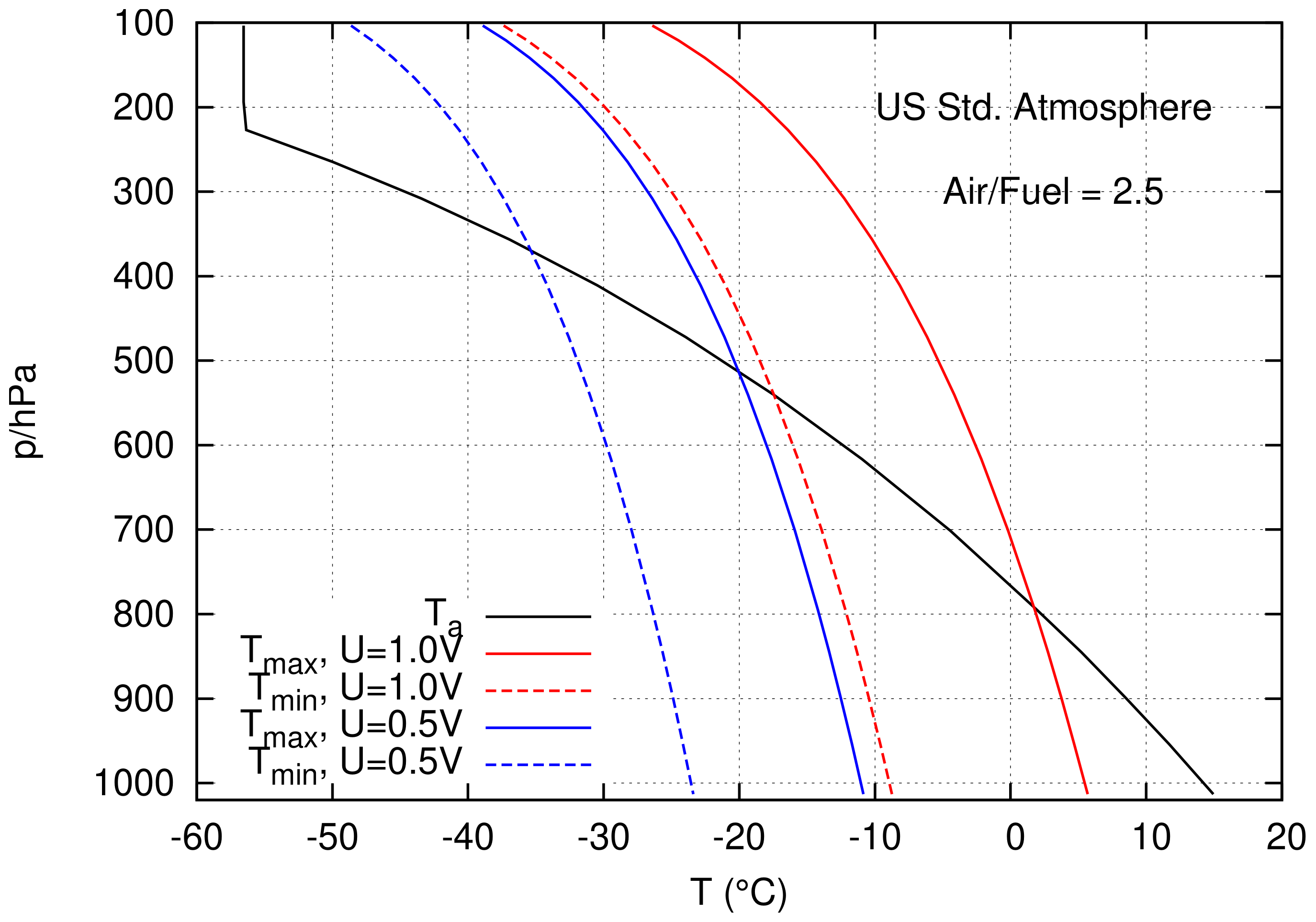
Figure 2 shows $T_{\max }\left(p_a\right)$ for $U=1$ V (solid red) and $U=0.5$ V (solid blue) together with the temperature profile of the US standard atmosphere (black) [22]. The stoichiometric air/fuel ratio of $2.5$ has been assumed. Lines for higher air/fuel ratios would appear very similar. In all cases, contrail formation is possible at much lower altitudes than for jet engines. The minimum altitude necessary for contrail formation decreases with increasing FC voltage, because higher voltage implies higher efficiency to drive the engine and hence a colder exhaust follows, which is more susceptible to contrail formation. With the higher voltage, contrail formation is possible even at ground if the ambient temperature falls to values below about 5 ${}^{\circ }$C.

There is another threshold, $T_{\min }$ (dashed lines), at which contrail formation occurs even in absolutely dry air. This is given as

$$T_{\min }=T_{\max }-e^{*}\left(T_{\max }\right)/G_{\mathrm{FC}}.$$

(22)

That is, at $T<T_{\min }$ contrail formation occurs always, at $T>T_{\max }$ never, and between these boundaries it depends on the relative humidity (see below). The lower thresholds, that is, below which contrails are always formed, are slightly above $-10$${}^{\circ }$C for the 1 V FC on ground. Thus, contrail formation at the ground in winter can occur frequently for such a FC. A lower voltage leads to a substantial reduction of these thresholds at the expense of efficiency.

Figure 2 also shows that under conditions of the US-Standard Atmosphere contrails are always formed above 380 hPa (about $7.5$ km). The mean temperature at that level is still a few degrees above the temperature where minute water droplets freeze spontaneously. Droplets formed under these conditions will likely evaporate. However, the limit for spontaneous freezing (ca. $-38$${}^{\circ }$C, see [23], sect. 4a) is not far away. At the usual cruise levels, fuel cells will generally produce contrails. Below $-38$${}^{\circ }$C the droplets will freeze and the contrail may be persistent then, if the ambient relative humidity exceeds ice saturation.

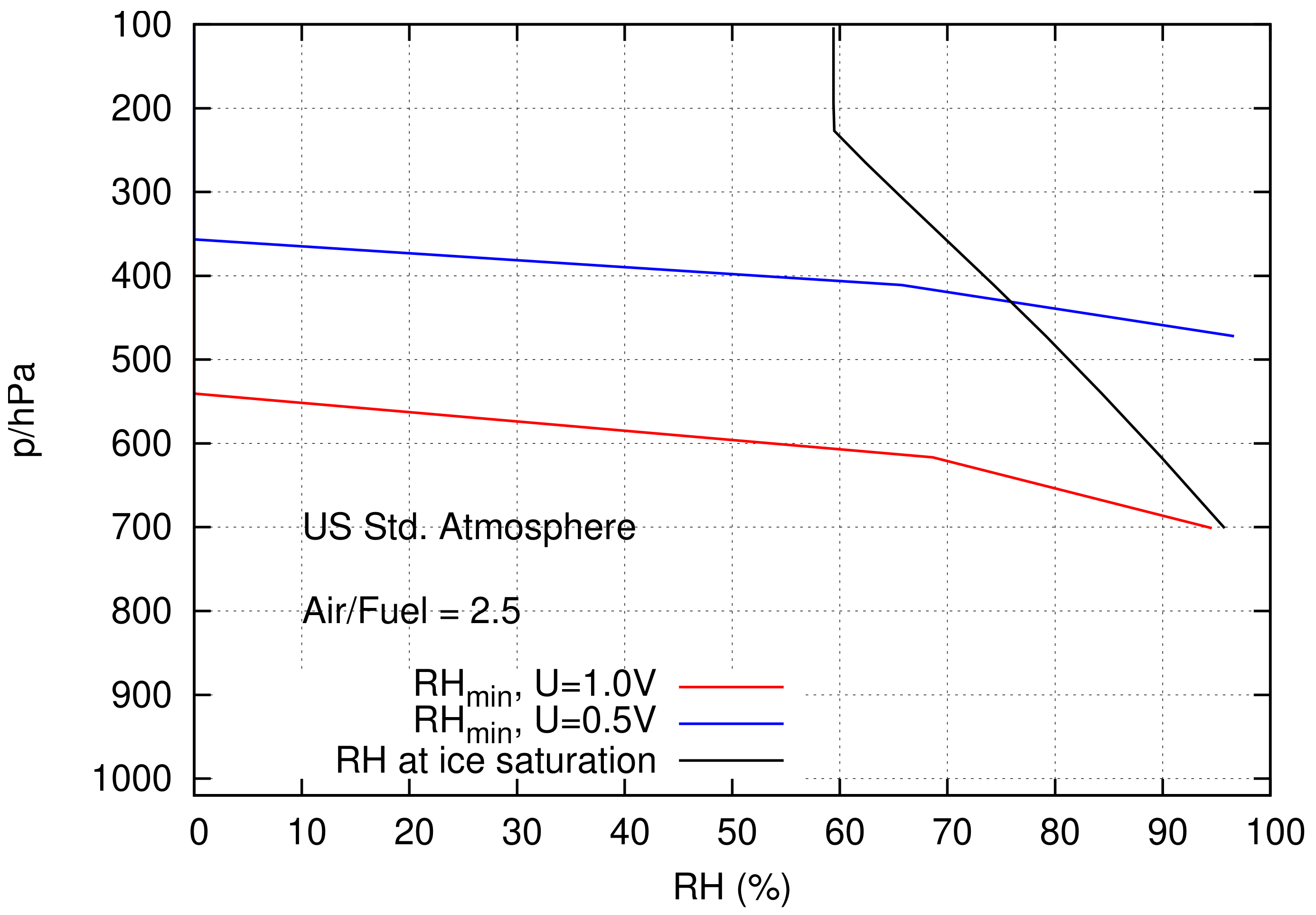
For temperatures between the upper and lower thresholds contrail formation requires a minimum relative humidity of the ambient air:

$$R{H}_{\min }\left(T\right)=\frac{e^{*}\left(T_{\max }\right)-G_{\mathrm{FC}}(T_{\max }-T)}{e^{*}\left(T\right)}.$$

(23)

Figure 3 shows for each pressure level the relative humidity required to produce a contrail (if the temperature actually is that of the assumed US standard atmosphere from Figure 2). Furthermore it displays for the same assumed temperature profile the relative humidity at which ice saturation is reached, which is the minimum required for contrail persistence. Again the curves are displayed for voltages of 1 V (red) and $0.5$ V (blue).

2.7. Comparison to Hydrogen Burning in a Gas Turbine

The burning of gases in a gas turbine delivers expansive work that finally drives the turbine. The reaction enthalpy of the combustion reaction equals the expansive work done by the reacting gases under conditions of constant pressure and temperature. (It may sound surprising to invoke the condition of constant temperature, but once the engine is switched on the temperature rises until it attains a constant high value when the engine runs continuously.) Hence the relevant energy for a gas turbine is $\Delta h$. The temperature in a combustion chamber is much higher than 100 ${}^{\circ }$C, such that the product of burning hydrogen is water vapour, and the relevant enthalpy is the lower heating value that was already applied above, $\Delta h=-241.82$ kJ mol${}^{-1}$. The contrail factor for a hydrogen gas turbine is thus

$$G_{\mathrm{LH}2}=\frac{c_{p,\mathrm{air}}{p}_a}{(1-\eta )|\Delta h|},$$

(24)

where all quantities are given per mole. A more familiar form appears when the quantities are given per kg with $c_{p,\mathrm{air}}=1005$ J (kg K)${}^{-1}$ and $|\Delta h|=120.9$ MJ kg${}^{-1}$, $\epsilon =0.622$ and with the emission index of water vapour ${\mathrm{EI}}_{{\mathrm{H}}_2\mathrm{O}}=9$ kg(water vapour) per kg(liquid hydrogen):

$$G_{\mathrm{LH}2}=\frac{c_{p,\mathrm{air}}{p}_a}{\epsilon }\frac{{\mathrm{EI}}_{{\mathrm{H}}_2\mathrm{O}}}{(1-\eta )|\Delta h|}.$$

(25)

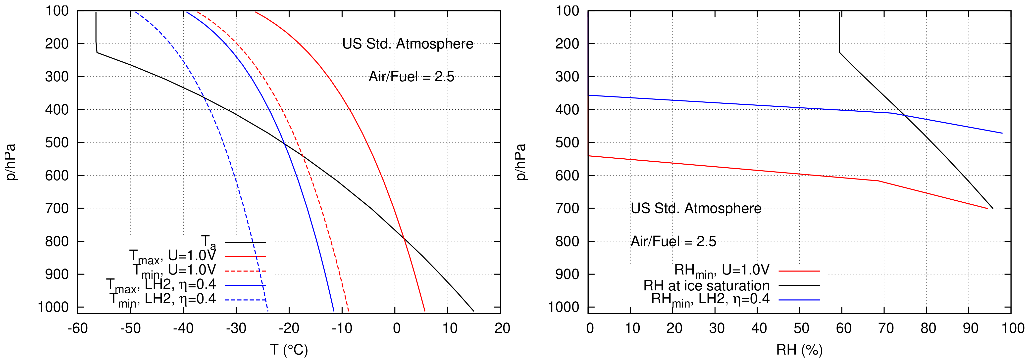
The G-factor for burning liquid hydrogen in a gas turbine is $2.6$ times larger than that for kerosene, if the overall propulsion efficiencies are equal. The thermal efficiency of the relevant Brayton cycle depends on the heat capacity ratio, $\gamma$, of the exhaust gas which in turn depends on the composition of the gas and thus on the amount of water vapour in the exhaust. However, the values of $\gamma$ differ little for water vapour (≈1.33) and air (≈1.4) and the water vapour fraction in the exhaust is small both for kerosene and for LH2. Thus the difference between the thermal efficiencies are small for the two types of fuel. Other components of the overall efficiency do not depend on the fuel.

Figure 4 shows a comparison of the contrail formation conditions for LH2 gas turbines with the hydrogen fuel cell. An overall propulsion efficiency of $0.4$ has been assumed for the gas turbine. It turns out that $T_{\max }$ for the LH2 gas turbine is lower then even $T_{\min }$ for the fuel cell operated at $U=1$ V, but the contrail formation conditions for the LH2 gas turbine are very similar to those of the FC at $0.5$ V, as a comparison with Figure 2 and Figure 3 shows.

3. Discussion

Aircraft with fuel cells will often resemble a steam engine, in particular in cold air, when taxiing at the airport. This is a sight one needs to accustom oneself to, but in terms of climate it is as harmless as steam clouds from real steam engines. Unless the steam droplets freeze, they will mostly evaporate within a few seconds since the air at ground is generally subsaturated. In fog the air might be saturated, but the additional droplets from a FC exhaust then just add to the fog droplets without noticeable effects for the radiation balance of the atmosphere.

It might be noticed that jet engines may produce such condensation at ground level as well. The G-factor for kerosene combustion from Equation (1) is about $7.8$ at $p_a=1000$ hPa, implying a temperature threshold of about $-24$${}^{\circ }$C. That is, at very cold locations it can be possible to see condensation occurring after jet engines at ground level. However, such condensation does not last longer than a few seconds and the author does not know any reports of such a phenomenon.

The situation is similar in the lower and middle troposphere as long as the droplets do not freeze. Perhaps one should avoid labelling such transient condensation phenomena contrails, because the notion “trail” implies something that is long, which will generally not be the case for transient condensation phenomena. The spontaneous freezing limit for small droplets is around $-38$${}^{\circ }$C, and as long as such a low temperature is not achieved the droplets will probably remain liquid. Outside of clouds the air is subsaturated and the droplets evaporate quickly. Aerodynamic overwing effects could lead to strong cooling, however [24,25,26], and thus the position of the exhaust pipe should be selected in a way that aerodynamic cooling does not occur. If the droplets condense on certain nuclei that are appropriate freezing nuclei, freezing can occur at temperatures higher than $-38$${}^{\circ }$C, but probably with small number densities [27].

At the usual cruise levels and also further above in the stratosphere contrail formation will always occur. The contrails will be short outside of ice supersaturated regions and many of them may remain subvisible, that is, they will not reach sufficient optical thickness to be visible for an observer at the ground. Contrails will only be persistent within ice supersaturated air. The frequency of ice supersaturation is a fundamental constraint for the coverage and occurrence frequency of all types of contrails.

Optical and microphysical properties of FC-contrails may differ a lot from contrails produced by jet engines. Calculations assuming ambient relative humidity with respect to ice of 130% indicate that the maximum saturation ratio (with respect to liquid water) that would be achieved by the expanding plume in the moment when it is cooled down to $T_{\max }$ is moderate, of the order 3–4 even when the fuel cell is driven with $U=1$ V and with the minimum air/fuel ratio of $2.5$. This means that condensation of liquid drops and freezing does not proceed spontaneously and needs ambient aerosol particles as condensation nuclei (see Figure 3 of [28] and references therein). This confines the number density of droplets and ice crystals to the number densities of ambient particles that are appropriate for condensation and freezing. These number densities are much smaller than the number densities of soot particles that are emitted by current jet engines. Contrails from FCs are thus more frequent but optically thinner than contrails from kerosene driven jet engines. In case of persistence, FC-contrails will on average have a shorter lifetime than contrails from kerosene combustion. As only persistent contrails play a role for climate impacts from aviation, it seems that replacement of kerosene driven gas turbines with fuel cells would be beneficial regarding contrails as well as regarding CO${}_2$ and further emissions of nitrogen oxides, sulphur oxides, soot and volatile aerosol.

4. Summary and Conclusions

The theory of contrail formation in the exhaust plumes of fuel cells is a variant of the well-known Schmidt-Appleman theory of contrail formation. It can be derived using the mass and energy balances to determine the slope $G_{\mathrm{FC}}$ of the (isobaric) mixing trajectory for the mixing of the exhaust gases with ambient air. The derivation presented in the current paper assumes the academic, but physically enlightening, case of unaltered exhaust gases. Real cases where the exhaust gases are led through heat exchangers and condensers cannot be treated with a general formula of the traditional form. Instead, once the static temperature and water vapour partial pressure are known at the exhaust exit and in the environment, engineers can start with Equation (2) (the definition of the G-factor) to compute G, use it in Equation (21) to determine the threshold temperature for contrail formation, and proceed with Equations (22) and (23) to determine whether the situation is sufficiently humid for contrail formation.

It turns out that the G-factor for FCs is much larger than that of conventional jet engines, because the amount of vapour emission is high and the static temperature of the exhaust gases can be relatively low. FCs can produce condensation phenomena even at the Earth surface if the weather is cold (close to frost). These are short-living phenomena, which will disappear after a few seconds (outside of fog) and thus the term “contrail” should not be used for such a transient phenomenon.

A fleet of aircraft equipped with FCs may produce condensation almost everywhere, from the lower troposphere up to the stratosphere. If the lifetime (and thus length) of the condensation trail is sufficiently long, it is justified to call them contrails. Mere condensation that is visible only for few seconds should not be called contrail. Below certain temperatures, which are not extremely low, contrail production from FCs appears unavoidable, even in otherwise very dry air, like in the stratosphere. In most cases, however, this should lead merely to strange views of the sky when many aircraft have a short trail of steam like a steam engine. These contrails should mostly be quite short and some of them even invisible to an observer at the ground. They should not have any noticeable impact on weather and climate.

Only in case of ice-supersaturation, where contrails are persistent, a contribution to aviation’s climate impact can be expected. However, contrails from fuel cells will probably have a lower number density of ice crystals than persistent contrails from kerosene engines. The ice crystals will then on average be larger and thus fall faster. This implies that persistent FC-contrails should have on average shorter lifetimes than contrails from kerosene gas turbines.

Regarding the fact that FCs produce no other emissions than air and water vapour, one can recommend the introduction of this technique for aviation from a climate perspective. Their contrails might turn out to be ubiquitous, but most of them are harmless, and the persistent ones are less climate effective than the contrails from the current fleet of kerosene driven aircraft. In any case, these predictions should be tested in numerical experiments and with research flights, and the climate impact of a fleet of aircraft equipped with fuel cells should be assessed using appropriate numerical tools.

References

1. Schmidt, E. Die Entstehung von Eisnebel aus den Auspuffgasen von Flugmotoren. Schriften Der Dtsch. Akad. Der Luftfahrtforsch. 1941, 44, 1–15. [Google Scholar]
2. Appleman, H. The formation of exhaust condensation trails by jet aircraft. Bull. Amer. Met. Soc. 1953, 34, 14–20. [Google Scholar] [CrossRef] [Green Version]
3. Schumann, U. On conditions for contrail formation from aircraft exhausts. Meteorol. Z. 1996, 5, 4–23. [Google Scholar] [CrossRef]
4. Teoh, R.; Stettler, M.; Majumdar, A.; Schumann, U.; Graves, B.; Boies, A. A methodology to relate black carbon particle number and mass emissions. J. Aerosol Sci. 2019, 132, 44–59. [Google Scholar] [CrossRef]
5. Kärcher, B.; Yu, F. Role of aircraft soot emissions in contrail formation. Geophys. Res. Lett. 2009, 36, L01804. [Google Scholar] [CrossRef] [Green Version]
6. Ström, L.; Gierens, K. First simulations of cryoplane contrails. J. Geophys. Res. 2002, 107, 4346. [Google Scholar] [CrossRef]
7. Lee, D.; Fahey, D.; Skowron, A.; Allen, M.; Burkhardt, U.; Chen, Q.; Doherty, S.; Freeman, S.; Forster, P.; Fuglestvedt, J.; et al. The contribution of global aviation to anthropogenic climate forcing for 2000 to 2018. Atmos. Env. 2020. [Google Scholar] [CrossRef]
8. Gierens, K.; Spichtinger, P.; Schumann, U. Ice supersaturation. In Atmospheric Physics. Background—Methods—Trends; Schumann, U., Ed.; Springer: Berlin/Heidelberg, Germany, 2012; Chapter 9; pp. 135–150. [Google Scholar]
9. Williams, V.; Noland, R.; Toumi, R. Air transport cruise altitude restrictions to minimize contrail formation. Clim. Policy 2003, 3, 207–219. [Google Scholar] [CrossRef]
10. Noppel, F.; Singh, R. An overview on contrail and cirrus cloud avoidance technology. J. Aircraft 2007, 44, 1721–1726. [Google Scholar] [CrossRef]
11. Gierens, K.; Lim, L.; Eleftheratos, K. A review of various strategies for contrail avoidance. Open Atmos. Sci. J. 2008, 2, 1–7. [Google Scholar] [CrossRef] [Green Version]
12. Gierens, K.; Matthes, S.; Rohs, S. How well can persistent contrails be predicted? Aerospace 2020, 7, 169. [Google Scholar] [CrossRef]
13. Haglind, F. Potential of lowering the contrail formation of aircraft exhausts by engine re–design. Aerospace Sci. Technol. 2008, 12, 490–497. [Google Scholar] [CrossRef]
14. Burkhardt, U.; Bock, L.; Bier, A. Mitigating the contrail cirrus climate impact by reducing aircraft soot number emissions. NPJ Clim. Atmos. Sci. 2018, 37, 1–7. [Google Scholar] [CrossRef] [Green Version]
15. Bier, A.; Burkhardt, U. Variability in contrail ice nucleation and its dependence on soot number emissions. J. Geophys. Res. 2019, 124, 3384–3400. [Google Scholar] [CrossRef] [Green Version]
16. Grewe, V.; Bock, L.; Burkhardt, U.; Dahlmann, K.; Gierens, K.; Hüttenhofer, L.; Unterstrasser, S.; Rao, A.; Bhat, A.; Yin, F.; et al. Assessing the climate impact of the AHEAD multi-fuel blended wing body. Meteorol. Z. 2016, 26, 711–725. [Google Scholar] [CrossRef]
17. Yin, F.; Grewe, V.; Gierens, K. Impact of hybrid electric aircraft on contrail coverage. Aerospace 2020, 7, 147. [Google Scholar] [CrossRef]
18. Atkins, P. Kurzlehrbuch Physikalische Chemie; Spektrum Akademischer: Heidelberg, Germany, 1993. [Google Scholar]
19. Kondepudi, D.; Prigogine, I. Modern Thermodynamics; John Wiley & Sons: Chichester, West Sussex, UK, 1998. [Google Scholar]
20. Srinivasan, S. Fuel Cells; Springer: New York, NY, USA, 2006; p. xxx + 691. [Google Scholar]
21. Busen, R.; Schumann, U. Visible contrail formation from fuels with different sulfur contents. Geophys. Res. Lett. 1995, 22, 1357–1360. [Google Scholar] [CrossRef] [Green Version]
22. Anderson, G.; Clough, S.A.; Kneizys, F.; Chetwynd, J.; Shettle, E. AFGL Atmospheric Constituent Profiles (0–120 km); Technical Report; AFGL-TR-86-0110, Air Force Geophys. Lab.; Hanscom Air Force Base: Bedford, MA, USA, 1986. [Google Scholar]
23. Murphy, D.; Koop, T. Review of the vapour pressures of ice and supercooled water for atmospheric applications. Q. J. Roy. Met. Soc. 2005, 131, 1539–1565. [Google Scholar] [CrossRef]
24. Gierens, K.; Kärcher, B.; Mannstein, H.; Mayer, B. Aerodynamic contrails: Phenomenology and flow physics. J. Atmos. Sci. 2009, 66, 217–226. [Google Scholar] [CrossRef]
25. Heymsfield, A.; Kennedy, P.; Massie, S.; Schmitt, C.; Wang, Z.; Haimov, S.; Rangno, A. Aircraft-induced hole punch and canal clouds. Bull. Am. Meteorol. Soc. 2010, 753–766. [Google Scholar] [CrossRef] [Green Version]
26. Heymsfield, A.; Thompson, G.; Morrison, H.; Bansemer, A.; Rasmussen, R.; Minnis, P.; Wang, Z.; Zhang, D. Formation and spread of aircraft-induced holes in clouds. Science 2011, 333, 77–81. [Google Scholar] [CrossRef] [PubMed] [Green Version]
27. Findeisen, W. Die kolloidmeteorologischen Vorgänge bei der Niederschlagsbildung (Colloidal meteorological processes in the formation of precipitation). Meteorol. Z. 1938, 55, 121–133. [Google Scholar] [CrossRef]
28. Jansen, J.; Heymsfield, A. Microphysics of aerodynamic contrail formation processes. J. Atmos. Sci. 2015, 72, 3293–3308. [Google Scholar] [CrossRef]
Figure 1. Dependence of the maximum temperature at which contrails are possible, T max , on the logarithm of G for values of G exceeding 2 Pa K 1 , which are typical for fuel cell exhausts. The red circles represent the values from the Clausius-Clapeyron equation, the black solid line represents the cubic fit.
Aerospace 08 00164 g001
Figure 2. Profiles of temperature from the ground to about 13 km altitude, or 100 hPa. The black line represents the US Standard Atmosphere. The red lines are T max (solid) and T min (dashed) for fuel cells with U = 1 V. The blue lines are the analogue for U = 0.5 V.
Aerospace 08 00164 g002
Figure 3. Profiles of the relative humidity required for contrail formation for the same temperature profile as in Figure 2 and for fuel cells with voltages of 1 V (red) and 0.5 V (blue). The black line represents the relative humidity at which ice saturation is reached. This is a function of temperature only and is not defined for temperatures above the freezing point of water.
Aerospace 08 00164 g003
Figure 4. Comparison of contrail formation conditions for fuel cells (red) and combustion of liquid hydrogen (LH2) in a gas turbine (blue). The left panel shows the temperature conditions and the right one the conditions on relative humidity as in Figure 2 and Figure 3 above.
Aerospace 08 00164 g004
Publisher’s Note: MDPI stays neutral with regard to jurisdictional claims in published maps and institutional affiliations.