Research on Task Satellite Selection Method for Space Object Detection LEO Constellation Based on Observation Window Projection Analysis

Abstract

Aiming at the task planning and scheduling problem of space object detection LEO constellation (SODLC) for detecting space objects in deep space background, a method of SODLC task satellite selection based on observation window projection analysis is proposed. This method projects the spatial relative relationships of the SODLC observation blind zone, observation range, and the initial spatial position of the objects onto the surface of the earth for detectable analysis of satellites and targets and binds the dynamic observation conditions to the satellite trajectory after projection calculation of the visible relationship between target changes. On this basis, combined with the features of SODLC with high orbital symmetry, the task satellite selection is divided into two steps: orbit plane selection and task satellite selection. The orbit planes are selected based on the longitude range of the ascending node with the geographic location of the targets, and the task satellites are selected according to the relative motion relationship between the satellites and the targets together with the constraints of observable conditions. The selection method simplifies the calculation process of scheduling and selecting task satellites. Simulation analysis prove the method has better task satellite selection efficiency. The method has high practical value for task planning and scheduling for event-driven SODLC.

1. Introduction

Several megaconstellation projects are in progress for global communications, which are rapidly launching thousands of satellites into low earth orbits. Megaconstellations may have a potential catastrophic impact [1] on the space debris environment [2]. The amount of debris may augment rapidly if the satellites are not removed from their orbit after end of life, which is usually short. The large number of satellites in adjacent orbits will also increase the risk of collisions, which may lead to a burst of space debris [3].

With the growing number of space objects and increasing risk of LEO collisions, space object detection LEO constellation (SODLC) has been proposed to work with ground-based sensor networks to enhance the capability of space object detection, tracking, and identification and to establish timely response globally for space emergency events such as collisions. Du et al. proposed three Walker analog constellations to build and maintain a catalog of 200,000 LEO space debris [4]. Snow et al. introduced an optimization method to the CubeSat constellation design problem for a space-based optical debris observation system in which the Walker delta constellation was adopted [5].

SODLC needs to complete real-time system response after emergency events such as collisions. With the dynamic relative position between satellites and the target, multiple satellites in the SODLC are required to coordinate and relay information in order to achieve full-range tracking of the target. Moreover, the satellite can determine the orbit of the target with an angles-only method [6]. Therefore, an appropriate satellite and sensor management strategy is needed [7]. Hu et al. proposed a multiobjective optimization framework for the optimal design of emergency observation constellations [8].

SODLC requires autonomous mission planning and sensor scheduling [9] on the satellite to achieve dynamic resource allocation for targets. An observation sequence for a specific target is formed, and different satellites are dispatched in turn to track and detect the target [10]. In the initial stage of an event being triggered, it is particularly important to quickly and accurately select satellites suitable for observation, which is key to a successful response.

At the same time, SODLC satellites are constrained by various observation conditions during target tracking. For example, for target detection, the field of view (FOV) requires a deep space background, so the line of sight (LOS) must be above the atmospheric limb; the observation distance is limited by the capability of sensors. These constraints must be used as the screening criteria for task-executing satellites in mission planning [11].

When the event is triggered, the satellite needs to screen the existing satellites in real time to form a task sequence. Yu et al. investigated the emergency scheduling problem and proposed a cooperation-oriented ant colony optimization algorithm (CO-ACO) to solve the observation sequence problem [12]. Existing methods mainly select candidate satellites by directly calculating the spatial visibility between the target and all satellites. However, constraints in the observation conditions lead to high computational complexity, high onboard resource consumption, and low timeliness of mission planning. Existing SODLC planning methods do not effectively use the inherent characteristics of SODLC and the satellite itself to optimize the selection process of task satellites.

Although the target is noncooperative, it has certain temporal and spatial uncertainty as an event trigger. Previous studies have fully considered the real-time coverage performance of time and space when designing SODLC [13]. In order to achieve balanced spatial double coverage and intersatellite links [14], the Walker constellation adopts a configuration with very high symmetry and periodicity of motion characteristics [15].

In this study, a method is proposed that analyzes and calculates the observation conditions depending on the projection of the target trajectory, satellite trajectory, undetectable range of the atmospheric limb constraints, and the maximum detectable distance of the observation distance onto the surface of the earth. At the same time, the task satellite selection is divided into two steps considering the high orbital symmetry, namely orbital plan selection and task satellite selection, which greatly simplifies the calculation process for task satellite selection. After the dynamic observation conditions are projected and bound to the satellite trajectory, the visible relationship with the target change can be precisely calculated, which serves for dynamic mission planning.

2. Problem Description

2.1. Ground Projection of the SODLC Satellite Observation Range

SODLC satellites need to observe the target in a deep space background above the atmospheric limb. Therefore, the LOS of the target should be at least tangent to the edge of the atmospheric limb, as shown in Figure 1.

The target cannot be observed when it appears in the range of the intersection ${\theta }_b$ of the line from the satellite to the center of the earth and the tangent of the satellite to the atmospheric limb.

An area centered on the subsatellite point and in range of $D_b$ is obtained by projecting the invisible observation angle range of the satellite to the target on the surface of the earth. A target is undetectable as long as its projection on the earth surface falls within the range above. The undetectable range $D_b$ is determined by the atmospheric limb height $H_a$, satellite orbit height $H_s$, and target height $H_{tar}^{}$.

$$\{\begin{array}{l}{D}_b(t)=\left[{\cos }^{-1}\left(\frac{{\mathrm{R}}_{\mathrm{e}}+H_a}{{\mathrm{R}}_{\mathrm{e}}+H_s}\right)-{\cos }^{-1}\left(\frac{{\mathrm{R}}_{\mathrm{e}}+H_a}{{\mathrm{R}}_{\mathrm{e}}+H_{tar}^{}\left(t\right)}\right)\right]\cdot {\mathrm{R}}_{\mathrm{e}},H_{tar}^{}\left(t\right)>H_a\\ D_b(t)=\left[{\cos }^{-1}\left(\frac{{\mathrm{R}}_{\mathrm{e}}+H_a}{{\mathrm{R}}_{\mathrm{e}}+H_s}\right)\right]\cdot {\mathrm{R}}_{\mathrm{e}},H_{tar}^{}\left(t\right)\le H_a\\ D_b(t)=0,H_{\mathrm{s}}\le H_a\end{array}$$

(1)

where R_e is the radius of the earth.

For a circular orbit, the orbital height of the satellite is regarded as a constant and the atmospheric limb height can also be considered as a certain value, while the height of the target changes with its movement. Therefore, the undetectable range will also vary with the height of the target. When the target height is lower than the atmospheric limb height, the undetectable area is completely determined by the atmospheric limb. When the target height is greater than the atmospheric limb height, the undetectable range changes dynamically with the target height.

At the same time, the detection capability affects the performance of orbit determination [16]. Flohrer et al. analyzed the performance of space-based optical system with a 20 cm aperture, 6° field of view, and flexible integration requirements [17].

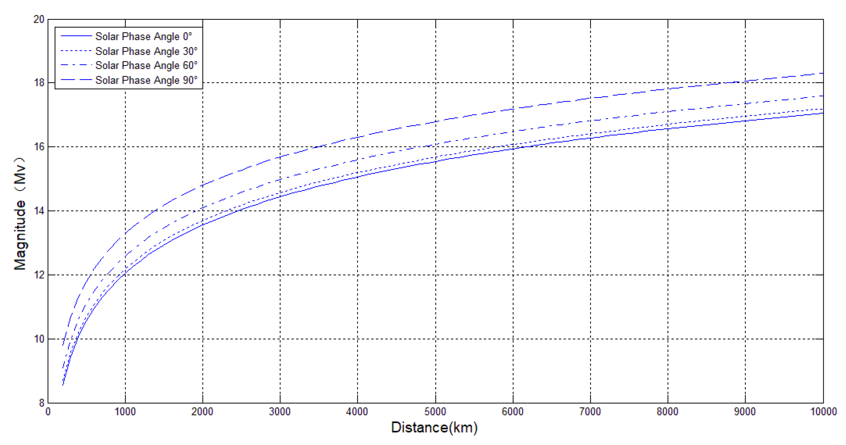
The detection capability is decided by the aperture, optical system efficiency, and integration time. In order to simplify the analysis of the problem, the target is calculated as a 10 cm diameter sphere, and the dimmest magnitude observable by the optical system studied is around 17.2 M_v with 15 cm aperture and flexible integration. The magnitude is calculated by Equation (2):

$$m=-26.58-2.5{\log }_{10}[A\gamma \mathrm{F}(\varphi )/L^2]$$

(2)

where

• m is the limiting magnitude;
• A is area of the space object along the line of sight;
• $\gamma$ is the reflectivity;
• $\mathrm{F}(\varphi )$ is the solar phase angle; and
• L is the observation distance.

The calculation results are in Figure 2.

In Figure 2, with the dimmest magnitude of around 17.2 M_v in this study, the maximum detection distance is 6000 km.

Because the SODLC satellite has azimuth omnidirectional maneuverability, the connection between the farthest point of detection and the center of the earth will also form a range on the ground with the subsatellite point as the center and D as the arc length, where D is the maximum range projection of the observation. After eliminating the projection of the undetectable area, the detectable area is an annulus with a width of D_l.

$$\{\begin{array}{l}D(t)={\cos }^{-1}\left[\frac{{\left({\mathrm{R}}_{\mathrm{e}}+H_{tar}^{}\left(t\right)\right)}^2+{\left({\mathrm{R}}_{\mathrm{e}}+H_s\right)}^2-L^2}{2\cdot \left({\mathrm{R}}_{\mathrm{e}}+H_{tar}^{}\left(t\right)\right)\cdot \left({\mathrm{R}}_{\mathrm{e}}+H_s\right)}\right]\cdot {\mathrm{R}}_{\mathrm{e}},H_{tar}^{}\left(t\right)>H_a\\ D(t)=0,H_{tar}^{}\left(t\right)\le H_a\end{array}$$

(3)

Similarly, the maximum length of the observable range $D(t)$ also varies with the $H_{tar}^{}\left(t\right)$ height of the target. When $H_{tar}^{}\left(t\right)$ is less than the atmospheric limb, there is no detectable range, i.e., $D(t)$ is 0.

The width of the detectable ring zone is as follows:

$$D_l\left(t\right)=D(t)-D_b(t),H_{tar}^{}\left(t\right)>H_a$$

(4)

Above, a ring-shaped detectable area projected onto the earth’s surface is formed by the constraints of the atmospheric limb observation and the maximum observation distance.

2.2. Dynamic Detectability Analysis of Targets

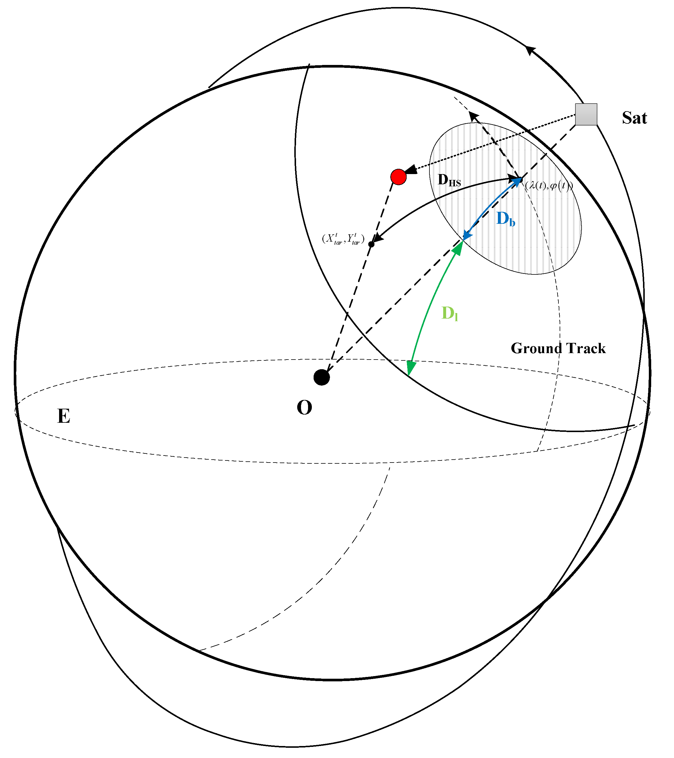
Because the spatial positions of the target and the satellite are in a highly dynamic process, the visibility of a target to a specific satellite should be judged under a dynamic condition. Therefore, it is necessary to combine the undetectable area $D_b(t)$ centered on the satellite’s subsatellite point with the detectable area $D_l\left(t\right)$ and the satellite’s subsatellite point trajectory to form a judgment on the detectability condition of a specific target at a specific time. The relationship between the projection point of the target on the earth’s surface and the projection of different detection characteristics is shown in Figure 3.

For the target, at a given time t, the target’s geographic longitude $X_{tar}^t$, geographic latitude $Y_{tar}^t$, and target height $H_{tar}^{}\left(t\right)$ are all determined.

Similarly, at a given time t, the geographic longitude $\lambda (t)$ and geographic latitude $\phi \left(t\right)$ of the subsatellite point of a specific satellite Sat are also determined, and the satellite height is still considered as a fixed value.

For a certain orbit, the geographic longitude $\lambda (t)$ and geographic latitude $\phi \left(t\right)$ of the subsatellite point are determined by the inclination of the satellite orbit and the true anomaly at time t.

The calculation formula for the geographic longitude of the satellite subsatellite point is as follows:

$$\lambda (t)={\mathsf{\Omega }}_{g0}+\arctan \left[\cos i\tan \left(\omega +\theta (t)\right)\right]$$

(5)

The calculation formula for the geographical latitude of the satellite subsatellite point is as follows:

$$\phi \left(t\right)=\arcsin \left[\sin i\sin \left(\omega +\theta \left(t\right)\right)\right]$$

(6)

Among them, the orbit inclination i is a fixed value for determining the orbit, and ω is a fixed value for the argument of perigee.

The true anomaly at a specific time t is as follows:

$$\theta (t)={\theta }_0+nt$$

(7)

where θ₀ is the true anomaly at the initial moment (epoch).

$$n=\sqrt{\frac{\mu }{a^3}}$$

(8)

where $a$ is the semimajor axis of the orbit, and $\mu$ = 3.986006 × 10⁵ km³/s².

At a specific time t, the arc length $D_{\mathrm{HS}}$ between the subsatellite point on the earth’s surface and the target projection point can be calculated as follows:

$$D_{\mathrm{HS}}\left(t\right)={\mathrm{R}}_{\mathrm{e}}\cdot {\cos }^{-1}\left[\cos (Y_{tar}^t)\cos (\phi \left(t\right))\cos (X_{tar}^t-\lambda (t))+\sin (Y_{tar}^t)\sin (\phi \left(t\right))\right]$$

(9)

where $\lambda (t)$ is the geographic longitude and $\phi \left(t\right)$ is geographic latitude of the specific satellite Sat’s subsatellite point, $X_{tar}^t$ is the geographic longitude and $Y_{tar}^t$ is geographic latitude of the target.

According to the length of the arc connecting the subsatellite point and the target projection point, it can be judged whether it is in the detectable area. If DET stands for the number of satellites that have conditions for observing a specific target,

$$\{\begin{array}{l}DET=1,D_b(t)<D_{HS}(t)\le D_l(t)\\ DET=0,D_{HS}(t)\le D_b(t)\cup D_{HS}(t)>D_l(t)\end{array}$$

(10)

then, when the length of the arc connecting the subsatellite point and the target projection point $D_{\mathrm{HS}}\left(t\right)$ is greater than the undetectable arc $D_b(t)$ and less than the maximum detection distance arc $D_l(t)$, the DET count equals 1.

3. Task Satellite Selecting Method

3.1. Analysis of the Relative Relationship between the SODLC and the Target

The SODLC adopts the Walker constellation. In this study, the 24/4/1 constellation configuration was chosen for the simulation analysis. The specific parameters of the seed Satellite1 can be seen in

Table 1. Orbital parameters of Satellite1.

Parameters	Value
Semimajor axis	7978.14 km
Eccentricity	1.47826 × 10−15
Inclination	60°
RAAN	1.11991 × 10−17°
Argument of perigee	0°
True anomaly	0°

.

The main constraints considered include the observation height of the atmospheric limb, the maximum detection distance, etc. The main simulation input parameters are shown in

Table 2. Simulation configuration parameters.

Parameters	Value
Atmospheric limb height	80 km
Maximum detection distance	6000 km
Satellite pointing range	Azimuth 360°, pitch ± 85°

.

3.2. Task Satellite Selection Method Based on Observation Window Projection

For the constellation, the target will have visibility to multiple satellites, especially the target with a long trajectory. Therefore, multiple satellites are required to complete the relay tracking of the target during its flight. After a target appears, the system needs to perform task planning and resource scheduling and then select the task satellites.

The existing method of selecting task satellites for the SODLC is to calculate the visibility and space observation constraints of the target and all satellites in orbit after the target appearance and then complete the task satellite selection after sorting according to the calculation results. The calculation is more complicated due to the dynamic characteristics of the satellite, the target, the constraints themselves, and the inherent characteristics of the satellite orbit, which are not fully considered to optimize calculation. In this paper, a method of projecting and screening task satellite observation windows is specially proposed. At the same time, the inherent characteristics of the constellation orbit and the relative relationship between the target and the satellite projected to the ground are used to quickly select task satellites. This method reduces unnecessary computing overhead and is adaptive to the task planning and resource scheduling process for dynamic changes.

Because the SODLC generally uses fewer orbital planes, analyses in the related literature have also used 3 to 4 orbital planes [18]. For each orbital plane, no matter how many satellites are distributed on this orbital plane at the time, the ascending node longitudes of all satellites on the same orbital surface are distributed in a specific interval at this specific time [19].

${\mathrm{R}}_{\mathsf{\Omega }}$ is the width of distribution interval for the ascending or descending nodes of all tracks in an orbital period.

$${\mathrm{R}}_{\mathsf{\Omega }}=T\cdot {\omega }_e$$

(11)

where T is the orbital period of the orbital plane, and ${\omega }_e$ is the earth’s rotation speed. For example, for an orbit with an orbit height of 1600 km and an orbital inclination of 60 degrees, the longitude of the satellite’s ascending node in an orbit is distributed in a longitude interval with a width of 29.549°. Based on the characteristics of the SODLC, the candidate orbital plane can be quickly selected by judging the distribution relationship between the target and the geographic longitude of the ascending node of the orbit. After the specific orbital plane is selected, the relative motion relationship between the target and the satellite can be used to select the candidate orbital plane and then the candidate observation satellites.

3.3. Orbit Plane Selection

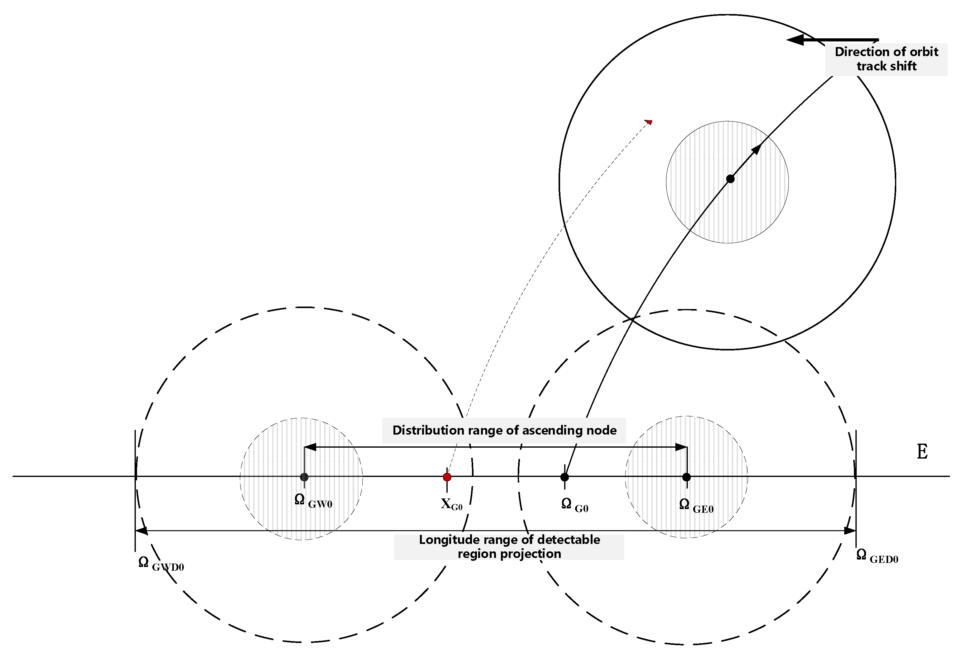
From Formula (10), a distribution interval of the ascending node longitude of the orbital plane is obtained. To compare the target and this interval, it is necessary to compare the position of the target and the position of the orbital interval on the equator, as shown in Figure 4.

The geographical longitude distribution range of the ascending node of the orbital plane can be calculated by the instantaneous root of any satellite in the orbital plane.

The calculation of the ascending orbit is shown in Formula (12):

$$\{\begin{array}{l}{\mathsf{\Omega }}_{G0}={\lambda }_0-\frac{{\mathrm{a}}^2}{{\mathrm{b}}^2}\tan {\phi }_0\mathrm{ctan}i\\ {\mathsf{\Omega }}_{GE0}={\mathsf{\Omega }}_{G0}-{\omega }_e\cdot \frac{{\theta }_0}{2\pi }\cdot T\\ {\mathsf{\Omega }}_{GW0}={\mathsf{\Omega }}_{G0}+{\omega }_e\cdot \left(1-\frac{{\theta }_0}{2\pi }\right)\cdot T\\ {\mathsf{\Omega }}_{G\mathrm{C}0}={\mathsf{\Omega }}_{GW0}-\frac{1}{2}\cdot {\mathrm{R}}_{\mathsf{\Omega }}\end{array}$$

(12)

The calculation of descending orbit is shown in Formula (13):

$$\{\begin{array}{l}{\mathsf{\Omega }}_{G0}={\lambda }_0+{180}^{°}+\frac{{\mathrm{a}}^2}{{\mathrm{b}}^2}\tan {\phi }_0\mathrm{ctan}i\\ {\mathsf{\Omega }}_{GE0}={\mathsf{\Omega }}_{G0}+{180}^{°}+{\omega }_e\cdot \frac{{\theta }_0}{2\pi }\cdot T\\ {\mathsf{\Omega }}_{GW0}={\mathsf{\Omega }}_{G0}+{180}^{°}-{\omega }_e\cdot \left(1-\frac{{\theta }_0}{2\pi }\right)\cdot T\\ {\mathsf{\Omega }}_{G\mathrm{C}0}={\mathsf{\Omega }}_{GW0}-\frac{1}{2}\cdot {\mathrm{R}}_{\mathsf{\Omega }}\end{array}$$

(13)

where ${\mathsf{\Omega }}_{G0}$ is the geographic longitude of the satellite’s ascending node, ${\mathsf{\Omega }}_{GE0}$ is the east extreme value of the longitude interval, ${\mathsf{\Omega }}_{GW0}$ is the west extreme value of the longitude interval, and ${\mathsf{\Omega }}_{G\mathrm{C}0}$ is the middle value of the longitude interval. a = 6356.755 km is the polar radius of the earth, and b = 6378.140 km is the equatorial radius. ${\theta }_0$ is the true anomaly of the satellite for the initial state, ${\lambda }_0$ is the longitude at the time, and ${\phi }_0$ is the latitude at the time. At this moment, we assume that the geographic location of the target has a virtual satellite, calculate the geographic longitude of the virtual satellite’s ascending node, obtain the projection of the target on the equator $X_{G0}$ that characterizes the orbital plane characteristics of the constellation, and calculate the difference between the center of each orbital surface distribution range and $X_{G0}$, filtering the track surface corresponding to the minimum value $\left|X_{G0}-{\mathsf{\Omega }}_{G\mathrm{C}0}\right|$.

3.4. Task Satellite Selection Analysis

After selecting the orbital planes, it is necessary to select candidate satellites on the selected orbital planes. The selection of candidate satellites is mainly based on the relative motion relationship between the satellite and the target with the constraints of observation conditions.

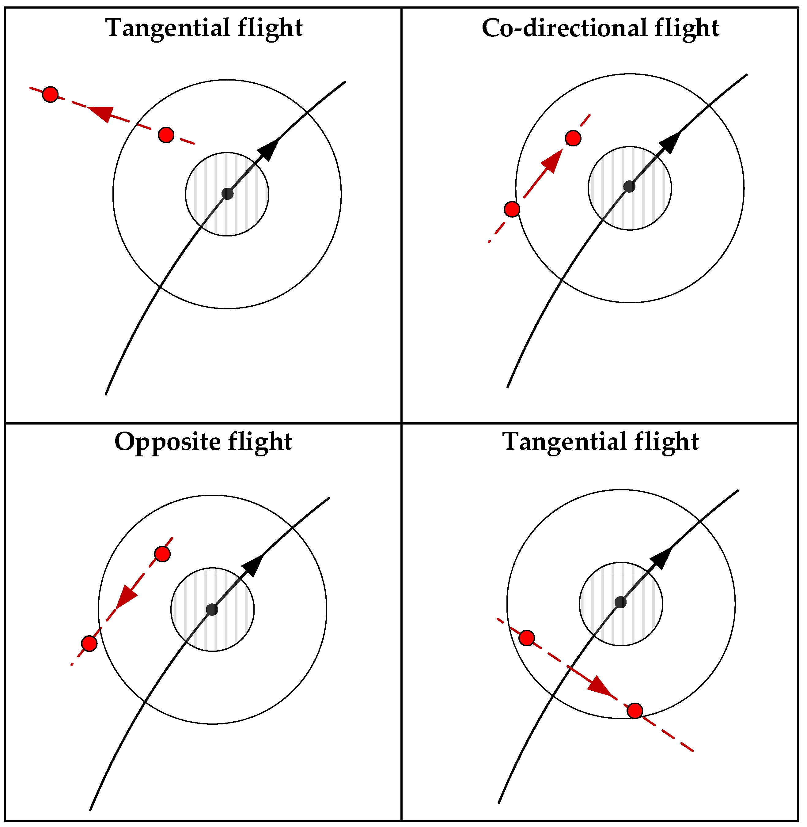
To summarize the relative motion relationship between the target and the satellite, the main situation can be seen in Figure 5. The target and the satellite are moving in completely opposite directions called opposite flight. While they are moving in the same direction called codirectional flight. The tangential horizontal flight can be divided into two situations with the same latitude and longitude deviation.

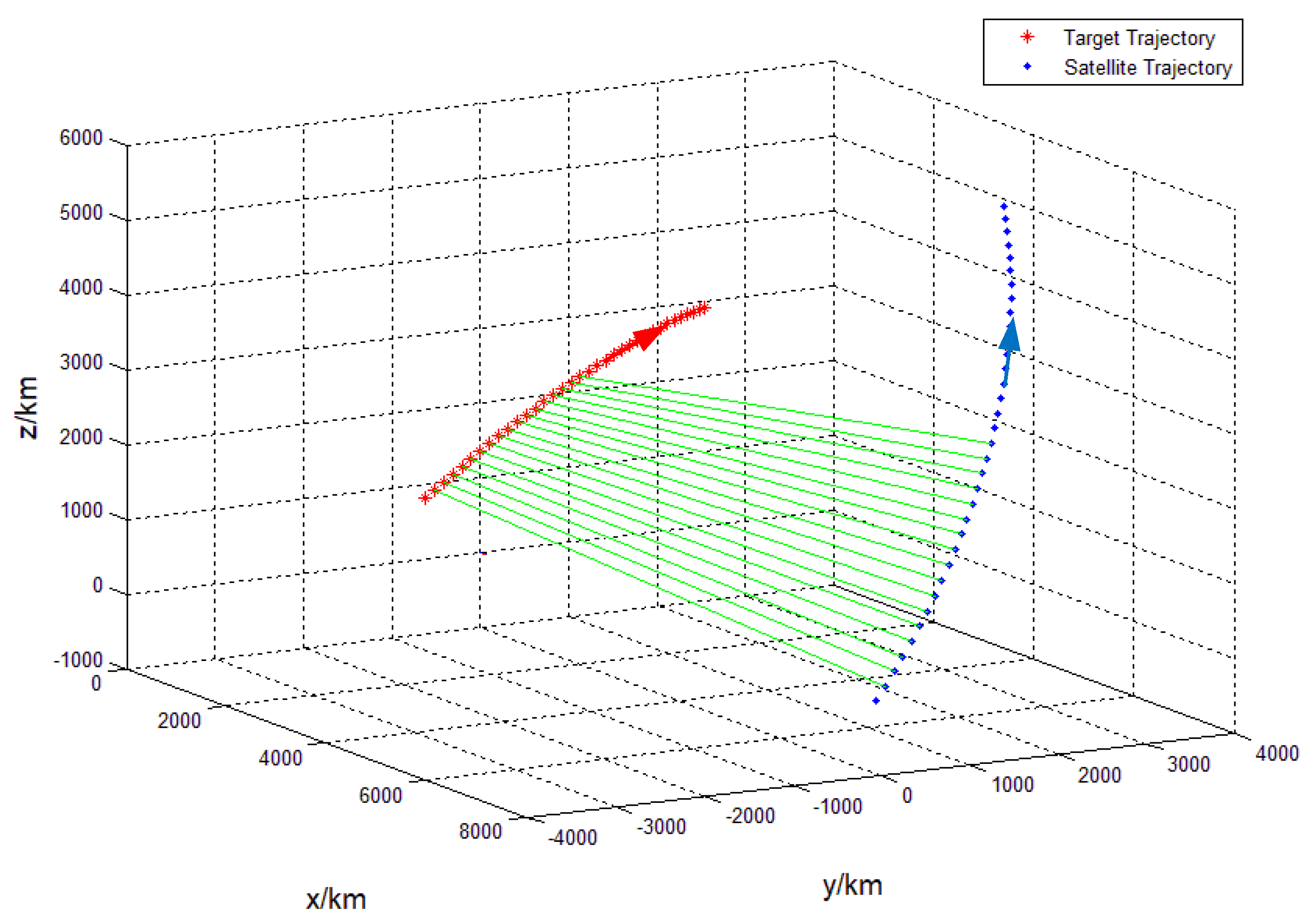
3.4.1. Codirectional Flight

The situation of the satellite and the target flying in the same direction can be seen in Figure 5. For time-sequence trajectories, the high-precision orbit propagator (HPOP) was adopted in the simulation. However, trajectory propagation is not the main research component of this article, and the propagation time was less than 1 h. Therefore, the model was simplified, the space targets were calculated as a 10 cm diameter sphere, and the satellites were calculated as an 80 cm cube.

In Figure 6, the red spots represent the space trace of the target, the blue spots denote the space trace of the satellite, and the green line is the line of sight. It can be seen from the figure that the satellite can detect the target almost all the way, the range of LOS adjustment is very small, and the observation conditions are better.

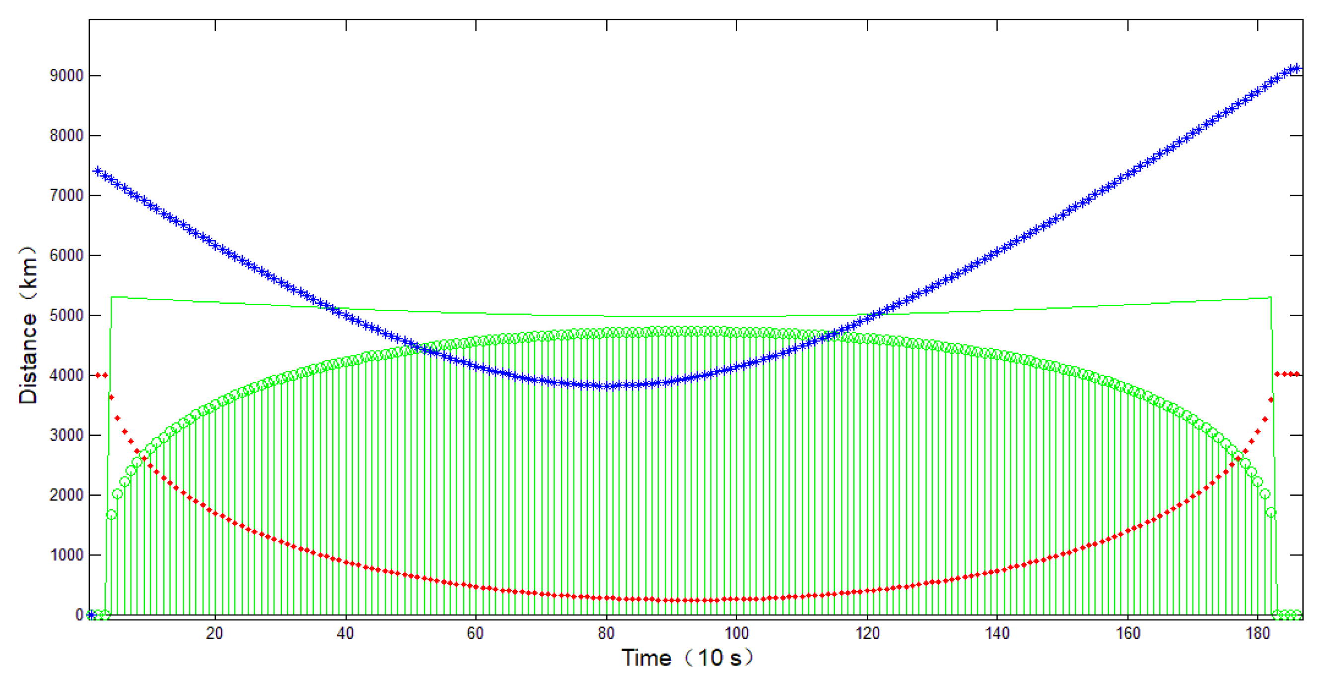
The changes in observation conditions during the observation process can be seen in Figure 7, where the green line is the maximum observation projection distance, the red line is the undetectable projection distance, and the blue line is the projection distance between the satellite and the target. The green area is the width of the observable area. It can be seen from the figure that the distance between the target and the satellite stays in the observable area between the maximum observation and the unobservable projection distance until the target height continues to decrease to unobservable.

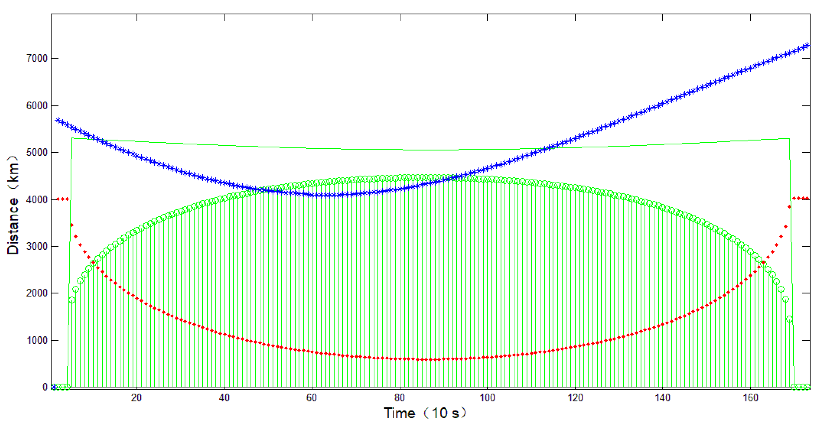
3.4.2. Tangential Flight

The situation of the tangential flight between the satellite and the target can be seen in Figure 8, Figure 9 and Figure 10, respectively. They are the deviation of longitude and latitude in the same direction and the deviation of latitude and longitude in the same direction. The first case can be seen in Figure 8. Only part of the arc of the target can be detected by the satellite.

The changes in observation conditions during the observation process can be seen in Figure 9 for this case. The main constraint on the length of the observation arc is that the distance between the satellite and the target exceeds the maximum observable distance.

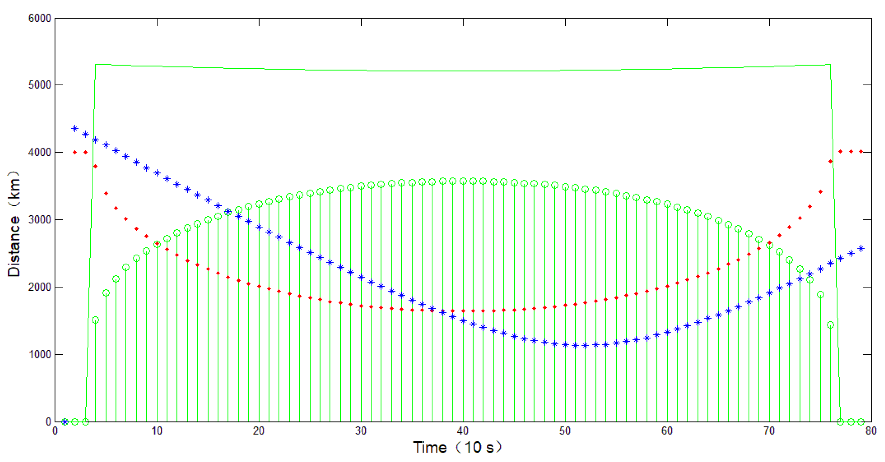
In Figure 10 and Figure 11, it can be seen that the same observation arc is limited when the latitude and longitude deviate in the same direction, and the main constraint comes from the observation distance, which exceeds the maximum observation distance. The observation efficiency of tangential direction flight is lower than that of the same direction flight.

3.4.3. Opposite Directional Flight

The situation of the satellite and the target flying in the opposite direction can be seen in Figure 12.

From Figure 12 and Figure 13, it can be seen that in the case of opposite directional flight, the observable arc of the target is extremely limited, which is mainly due to the target quickly approaching and entering the unobservable area. Therefore, when flying in opposite directions, the observation benefit is the lowest.

3.5. Task Satellite Selection Factor

In the selected orbital plane, the weight of three factors are proposed [20]: the relative angle influence factor $Q^n{}_{ra}$ is obtained by analyzing the relative motion relationship between the target and the satellite, $Q^n{}_{dst}$ is obtained by analyzing the distance relationship between the target and the satellite, and $Q^n{}_{bd}$ is obtained by analyzing the relationship between the target and the unobservable area. The overall task satellite selection factor SF is calculated as follows:

$${\mathrm{SF}}_{sat}^n=w_{ra}\cdot Q^n{}_{ra}+w_{dst}\cdot Q^n{}_{dst}+w_{bd}\cdot Q^n{}_{bd}$$

(14)

where $w_{ra}$ is the weight for the relative motion relationship, $w_{dst}$ is the weight for the relative distance observation, and $w_{bd}$ is the weight for the blind zone. Observing a target requires no less than two satellites at the same time, and considering the continuity of the entire process, two orbital planes and two satellites on the orbital plane were selected at the initial stage of selection. The selection factors of each satellite were calculated in the orbital plane, and the satellite with the highest factor value was selected as the first choice, while the satellite with the second highest choice factor was chosen as the second choice. The Monte Carlo simulation was used to determine the weight values. The simulation was divided into two stages. In the first stage, the satellites were selected with 0.1 as the weight step value for all three weights. Then, the length of the observation windows were calculated between 10 random targets and the selected satellite. After 10,000 iterations, a selection result with a length of 0.1 weight interval was obtained based on the longest observation window. In the second stage, the weight step setting was 0.01 in the chosen weight interval, and another 10,000 iterations were carried out to determine the weight settings, as seen in

Table 3. Weight configuration.

Weight	Value
Relative motion weight	0.14
Relative distance weight	0.65
Blind zone influence weight	0.21

.

4. Results and Discussion

Different latitudes and different moving trajectory targets were used to simulate and verify the screening method of the constellation. The main parameters of the target used in the simulation verification are shown in

Table 4. Coordinate of the trajectory shadow ends.

Target and Position	Longitude	Latitude
Target1 Position1	−143.505	38.230
Target1 Position2	−145.707	36.227
Target2 Position1	145.966	15.569
Target2 Position2	142.945	17.621
Target3 Position1	−118.793	41.002
Target3 Position2	−126.851	38.689
Target4 Position1	115.154	40.315
Target4 Position2	118.583	50.013

. The mid-latitude opposing flying target, the low-latitude tangential flying target, the mid-latitude tangentially biased remote target, and the high-latitude long-range target flying in the same direction were selected to simulate the selection of candidate orbits and task satellites.

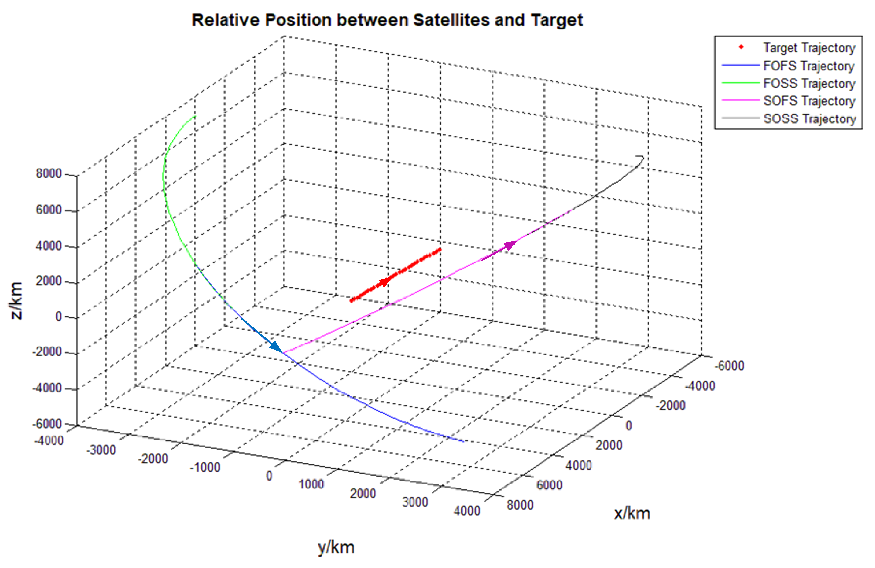
The selection results of candidate orbits and task satellites for the mid-latitude opposing flying target (target 1) can be seen in Figure 14. Among them, the satellite flying in the opposite direction of the target (the trajectory in purple-red line) had an observation window for the satellite. When flying in the opposite direction, it was the first satellite of the second selected orbit (SOFS), and the second selected satellite in second selected orbit (SOSS) with the black line in the trajectory had the ability to observe the target early. The blue trajectory was the first satellite of the first orbit (FOFS), which had the longest observation arc to the target. The green trajectory followed as the first orbit second satellite (FOSS). Although flying tangentially to the target, it had a better observation window due to the relative distance from the further point to the near point. The optimization results of orbits and task satellites were consistent with the actual observation conditions.

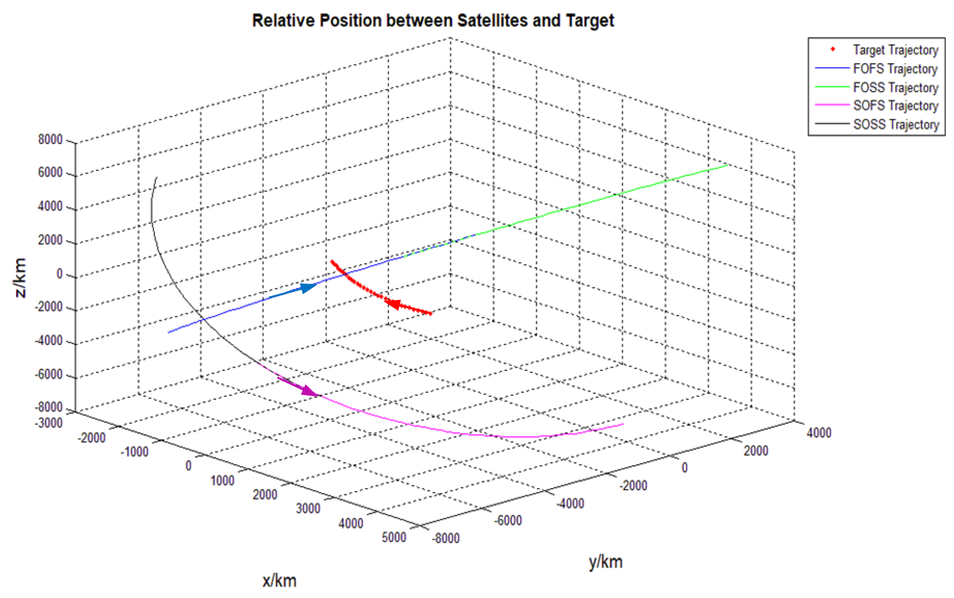
Figure 15 shows the satellite selection results of tangential flying targets at low latitudes. The target was tangential to the first orbit and opposite to the second orbit. Therefore, the selection results were consistent with the actual observation conditions.

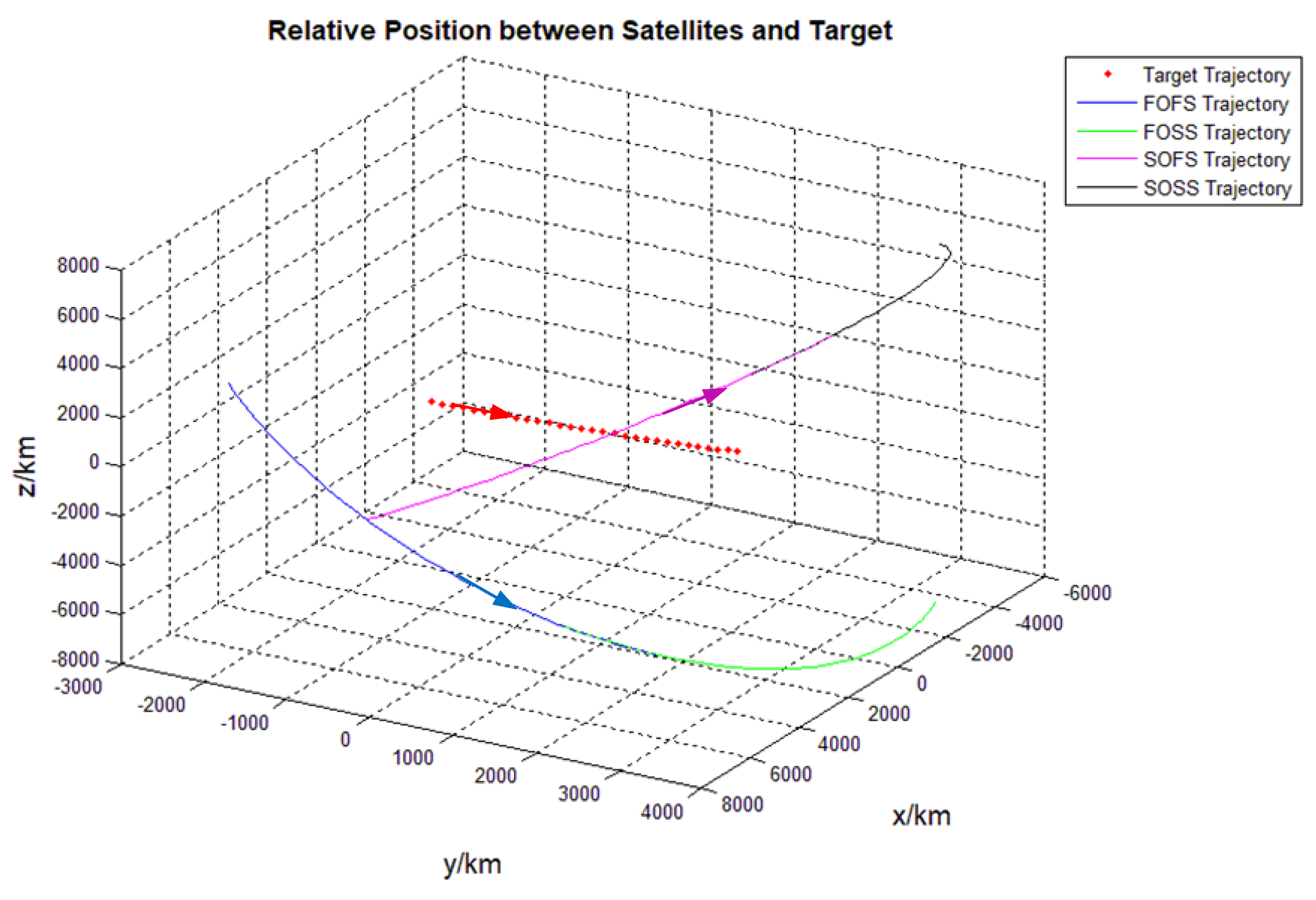
Figure 16 shows the satellite selection results of the mid-latitude long-distance flying target, the opposing flight orbit was selected as the first orbit, although there were fewer observing blind spots in the opposite direction. The four selected satellites were also the satellites with the best observation conditions under actual analysis.

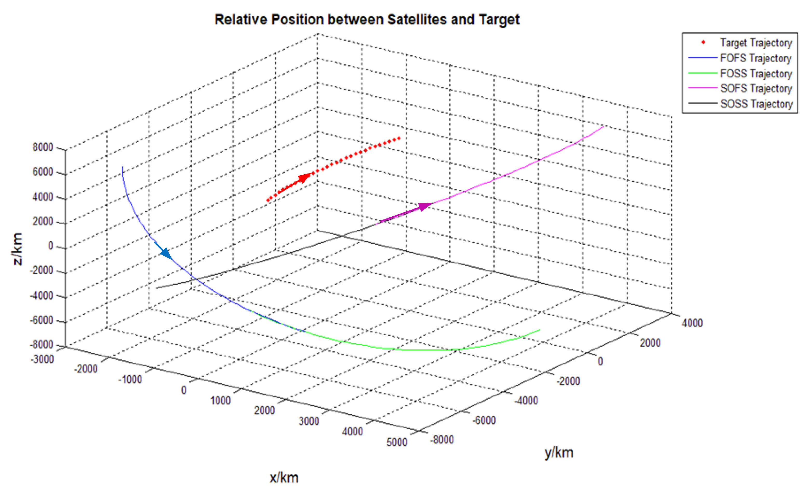
For high latitude target 4, the satellite selection result is shown in Figure 17. The orbit that actually had the longest observation window was selected as the suboptimal orbit. The selected four satellites were the four satellites with the best actual observation conditions, but there were discrepancies in the orbit and satellite ordering. The results showed that the selection of orbital planes based on the longitude of the ascending node was more sensitive to the latitude distribution of the target. The reason for this is that the input constellation orbits were densely distributed in high-latitude regions, and the observation conditions of each orbital plane were less different; therefore, optimally and suboptimally, the actual observational gain difference on the orbital surface was close. Therefore, although the order of satellite selection was different from the actual one, the selected satellite was the one with the best observation profit.

5. Conclusions

This study proposes a method that fully considers the constellation orbit characteristics for event-driven SODLC. After the target appears, based on the initial limited information, the candidate satellites with the observation conditions are quickly screened to meet the needs of high-efficiency mission planning and scheduling. The observation window projection screening method can quickly screen the observation satellites with better observation conditions through less calculation.

Calculation and simulation analysis show this method is able to select orbital planes with optimal observation conditions and the corresponding observation satellites when calculating mid-latitude and low-latitude targets. When calculating high-latitude area targets, the optimal satellites that are consistent with the actual observation benefits can be correctly selected, but there is a deficiency of insensitivity to the priority order of the orbital surface, which can be the subject of future optimization studies. The constraints considered in this work were mainly the atmospheric limb height and the observation distance, and more specific constraints such as the sun avoidance angle and full moon avoidance angle were not considered, which can also be studied in future work. The observation window projection screening method proposed in this paper has better task satellite selection efficiency, timeliness, and practical value for event-driven mission planning and scheduling of SODLC.