On-Orbit Pulse Phase Estimation Based on CE-Adam Algorithm

Abstract

Pulse phase is the basic measurements of X-ray pulsar-based navigation, and thus how to estimate a pulse phase for an orbiting spacecraft is important. The current methods for on-orbit pulse phase estimation could provide an accurate estimation performance enhancing with the photon amount, but its central processing unit (CPU) time cost also increases sharply with the increase of photon amount. In this paper, an on-orbit pulse phase estimation method based on the cross-entropy adaptive moment estimation (CE-Adam) algorithm is proposed to reduce the CPU time cost while retaining decent estimation accuracy. This method combines the CE and Adam algorithms, and is able to obtain a global optimum with low CPU time cost. The performance of the proposed algorithm is verified by simulation data and real data from the Neutron Star Internal Composition Detector (NICER). The results show that the proposed algorithm could greatly reduce the CPU time cost, which is about 1.5% of the CE algorithm, and retain similar estimation accuracy of pulse phase with CE algorithm.

1. Introduction

X-ray pulsar-based navigation (XPNAV) is a developing spacecraft autonomous navigation technique [1]. After being first introduced in 1981 [2], the past 40 years have witnessed a significant growth in XPNAV, including the pulse phase estimation as well as the navigation algorithm. Moreover, some flight experiments were performed such as SEXTANT (Station Explorer for X-ray Timing and Navigation Technology) [3] by the United States and the TG-2 (Tiangong-2) spacelab [4] and the Insight-HXMT (Insight-Hard X-ray Modulation Telescope) Satellite [5] of China.

Since the pulsar signal is extremely weak, an orbiting spacecraft can only record a series of photon TOAs (times of arrival) rather than a continuous pulsed signal [1]. Assuming the spacecraft is stationary or performs a uniform linear motion towards the pulsar, there are two types of method to estimate the pulse phase: the epoch-folding method [6] and the maximum likelihood estimator (MLE) method [7]. The epoch-folding method estimates pulse TOA by comparing the template with the empirical profile recovered by photon TOAs. Many methods based on epoch folding have been proposed in recent years. A wavelet-bispectrum algorithm is proposed in reference [8] to reduce the central processing unit (CPU) time cost of pulse phase estimation. In this method, wavelet transform is used to decompose the empirical profile and obtain low-frequency components of the empirical profile. Then, the low-frequency components are used to estimate the pulse phase [8]. In 2020, reference [9] proposed a genetic algorithm (GA)-optimized EMD (empirical mode decomposition)-CS (compressed sensing) with high accuracy and small computational load. In this method, the template is decomposed by the EMD (empirical mode decomposition) to obtain IMFs (intrinsic mode functions), and the IMFs selected by GA constitute the optimized measurement matrix. Then the pulse phase is estimated using the optimized measurement matrix [9]. In order to solve the sensitivity for noise, reference [10] proposed a variable step size iteration method which estimates pulse phase using a one-dimensional slice of template and empirical profile. The epoch-folding method is simple to implement, but needs lots of photons for the recovery of empirical profile and has an estimation accuracy less than MLE. However, the CPU time cost of MLE increases sharply as photon amount increases [7].

For orbiting spacecraft, the phase estimation problem become more complicated in that the orbit motion of a spacecraft introduces an unknown Doppler frequency into the pulse signal. To cope with this, Golshan et al. proposed a phase-tracking algorithm that divides the whole observation period into several short intervals [11]. During each interval, the spacecraft is approximated to perform a linear uniform motion, and in this case, the Doppler frequency is assumed to be constant and is tracked by a digital phase-locked loop (DPLL) [11]. In 2013, Huang et al. modified the DPLL to be a two-order Kalman filter and improve the performance of phase tracking [12]. In 2015, the phase tracking method was verified by the lab equipment of the Neutron Star Internal Composition Detector (NICER) and SEXTANT teams [13]. The phase tracking method works well for young pulsars such as PSR B0531+21(Crab) but fails when applied to faint millisecond pulsars such as PSR B1821-24 and PSR B1937+21. (The flux of Crab pulsar is 3667 photons/m²/s, but that of PSR B1937+21 is 0.161 photons/m²/s [14].) This is because the threshold for faint pulsars to obtain a reliable result is over 100 s, during which the assumption that a spacecraft performing a uniform linear motion is usually violated when the spacecraft is orbiting in a low Earth orbit. To overcome the drawbacks of the phase-tracking method, Wang and Zheng proposed a phase estimation method with the aid of orbital dynamics of spacecraft [15,16]. This method derives a linearized pulse phase propagation model, which modifies the pulse phase propagation model as a term of the position of the spacecraft. In addition, this method estimates the parameters of the linearized model to eliminate the impact of Doppler frequency. Compared with the phase-tracking algorithm, the phase estimation method with the aid of orbital dynamics of spacecraft does not divide the observation into intervals and thus is feasible for millisecond pulsar. Wang and Zheng recommend estimating the parameters by the direct search method [17]. Unfortunately, when using the direct search method, the CPU time cost is still high when the photon amount is large. In addition, Xue proposed estimating the Doppler frequency and pulse phase by a maximum likelihood estimator simultaneously [18], and this method also incurs high CPU time cost. Also, the photon background is an important factor which will impact on the performance of pulse phase estimation. Reference [19] shows that the photon background constantly changes because of orbital motion of the spacecraft. Reference [20] argues the effect of orbital motion on photon background could be reduced by data screening and the photon background could be assumed as a constant after data screening. Thus, in the existing methods, the photon background is assumed as a constant in the observation period.

For an on-orbit pulse phase estimation problem, there is a contradiction between estimation accuracy and CPU time cost. In order to estimate an accurate pulse phase, large amount of photons is needed, which leads to a high CPU time cost [21]. In reference [3], the error of position of XNAV is less than 10 km. In order to achieve this goal, the accuracy of phase estimation for Crab pulsar and PSR B1821-24 should be about 1 × 10⁻³ cycle. The linearized method could provide an accurate pulse phase estimation result with a high CPU time cost. According to the simulation results, the linearized method could obtain the pulse phase with enough accuracy when observation period is 1000 s. However, based on the computation environment of this paper, the CPU time cost of the linearized method is about 8000 s. This means that we can obtain the pulse phase of the first observation period after 8 observation periods, which is unacceptable for a navigation system. Thus, the CPU time of the pulse phase estimation method must shorter than the observation period. In addition, the position of spacecraft should be estimated using the estimated pulse phase. However, the CPU time cost by the pulse phase estimation might hinder the real-time navigation process. This is because the spacecraft keeps orbiting during the CPU time and the final estimated pulse phase reflects the position of the spacecraft before the CPU time. Thus, the CPU time cost by the pulse phase estimation should be as short as possible. To cope with this problem, we aimed to balance the pulse phase estimation accuracy and CPU time cost, which demands a highly efficient computational method with a decent estimation performance.

We cast the pulse phase estimation problem into a multi-extremal optimization problem. The cross-entropy (CE) algorithm is a classical method to solve a multi-extremal optimization problem, but has a heavy computational burden [22,23,24]. The Adam (adaptive moment estimation) algorithm is of high computational efficiency, but could only obtain a local optimum [25,26]. To combine the advantages of the two methods, this paper proposes a CE-Adam algorithm which features a low CPU time cost and global optimum. We compare the performance of the CE-Adam algorithm with the CE algorithm, DE (differential evolution) algorithm [27] and PSO (particle swarm optimization) [28] and find that the CE-Adam algorithm could provide accurate estimation results of pulse phase and significantly reduce the CPU time cost. In addition, we consider that the proposed algorithm could also be used to detect period signal in photon sequences over larger observational periods, which might indicate new physical phenomena.

The organization of this paper is as follows. Section 2 describes the principle of pulse phase estimation. Section 3 briefly reviews the CE algorithm and Adam algorithm. Section 4 shows the proposed CE-Adam algorithm. Simulation data and the real data are processed in Section 5 to verify the proposed algorithm. Finally, the summary of the conclusions is given in Section 6.

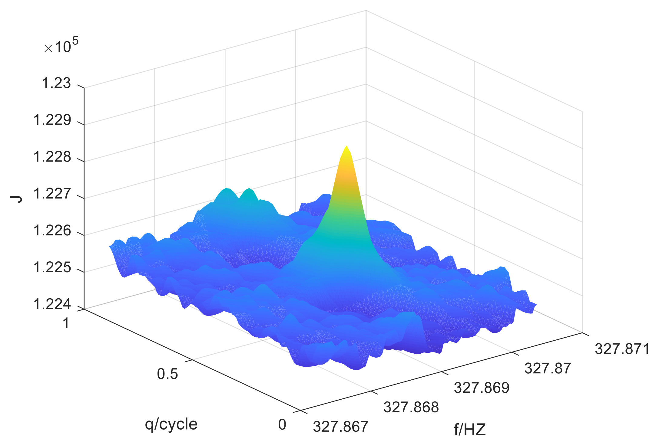
2. Principle of Pulse Phase Estimation

The arrival event of X-ray photons ${\left\{t_k\right\}}_{k=1}^N$ follows the non-homogeneous Poisson process. Within the interval $(t_a,t_b)$, the probability of k photons arrival is [29]:

$$P(k;(t_a,t_b))=\frac{e^{-(\overline{\mathsf{\Lambda }}(t_a)-\overline{\mathsf{\Lambda }}(t_b))}{(\overline{\mathsf{\Lambda }}(t_a)-\overline{\mathsf{\Lambda }}(t_b))}^k}{k!},$$

(1)

where $\overline{\mathsf{\Lambda }}$ satisfies $\overline{\mathsf{\Lambda }}(t)={\displaystyle {\mathrm{\int }}_0^t\mathit{\lambda }(s)ds}$. $\mathit{\lambda }$ is the rate function and can be given by:

$$\mathit{\lambda }(t)=\mathit{\lambda }(\varphi (t))=\beta +\alpha h(\varphi (t)).$$

(2)

The parameters $\alpha$, $\beta$ represent average signal and total background count rates in units of counts per second, respectively. $h$ is the normalized profile function of pulsar, $\varphi (t)$ represents the pulsar signal phase at the detector. $\varphi (t)$ can be expressed as [14]:

$$\varphi (t)={\varphi }_0(t-\tau (t)),$$

(3)

where ${\varphi }_0$ is the phase evolution at the reference observatory (we usually choose the Solar System Barycenter (SSB) as the reference observatory), and $\tau (t)$ represents the light propagation time from the detector to the reference observatory.

For an orbiting spacecraft, $\varphi (t)$ can be expressed as [14]:

$$\begin{array}{l}\varphi (t)={\varphi }_0\left(t-\frac{\mathit{x}(t)\cdot \mathit{n}}{c}\right)\\ ={\varphi }_0\left(t-\frac{\tilde{\mathit{x}}(t)\cdot \mathit{n}}{c}+\frac{\delta \mathit{x}(t)\cdot \mathit{n}}{c}\right)\\ \simeq \tilde{\varphi }(t)+{\dot{\varphi }}_0\left(t-\frac{\tilde{\mathit{x}}(t)\cdot \mathit{n}}{c}\right)\frac{\delta \mathit{x}(t)\cdot \mathit{n}}{c},\\ =\tilde{\varphi }(t)+e(t),\end{array}$$

(4)

where $\mathit{x}(t)$ is the spacecraft position vector, $\mathit{n}$ is the pulsar direction vector, $\mathit{x}˜(t)$ is the predicted position vector of spacecraft, $\delta \mathit{x}(t)=\tilde{\mathit{x}}(t)-\mathit{x}(t)$, $e(t)$ can be linearized as $e(t)=q+f(t-t_a)$, q is the initial phase at time $t_a$, and $f=\dot{\varphi }$ is the frequency of the pulsar signal.

According to Equation (4), $\varphi (t_k)$ can be expressed as:

$$\varphi (t_k)=\tilde{\varphi }(t_k)+q+f(t_k-t_a).$$

(5)

The joint probability density function of the pulsar photon arrival event is:

$$p(t_1,\cdots t_N,q,f)=e^{-{\displaystyle {\mathrm{\int }}_{t_a}^{t_b}\mathit{\lambda }(s)ds}}{\displaystyle \prod _{k=1}^N\mathit{\lambda }(t_k)}.$$

(6)

We define Equation (5) as the likelihood function. The natural logarithm of the likelihood function is:

$$J={\displaystyle \sum _{k=1}^N\ln \mathit{\lambda }(t_k)}-{\displaystyle {\mathrm{\int }}_{t_a}^{t_b}\mathit{\lambda }(s)ds}.$$

(7)

When the observation period is long enough, the second term in Equation (6) is a constant [29]. Thus, Equation (6) can be transformed into:

$$J={\displaystyle \sum _{k=1}^N\ln \mathit{\lambda }(t_k)}.$$

(8)

Parameters $q$ and $f$ can be estimated by solving the following optimization problem [14]:

$$(\widehat{q},\widehat{f})=\arg \underset{q,f}{\max }{\displaystyle \sum _{k=1}^N\ln \mathit{\lambda }(t_k)}.$$

(9)

The CRLB (Cramer–Rao lower bound) for estimation for q is given by [21]:

$$CRLB(q)=\frac{1}{T_{obs}{I}_p}$$

(10)

where $T_{obs}$ is the observation period and $I_p$ is a constant for each pulsar. It can be seen that the estimation accuracy of q is increased with observation period. As a result, large amounts of photons are needed for an accurate estimation of pulse phase. Equation (9) shows CPU time cost enhancing with the amount of photons. Thus, there is a contradiction between estimation accuracy and CPU time cost, and a computationally efficient algorithm with a decent estimation accuracy is needed.

As shown in Figure 1, the objective function shown as (8) has many extrema. Then, the gradient-descent technique could only arrive at a local optimum. Thus, a global optimization algorithm is needed.

3. Related Algorithm

3.1. Cross-Entropy (CE) Algorithm

Assume $S(x)$ is an objective function over all elements $x$ in $\chi$, and the maximum of it is ${\mathit{\gamma }}^{*}$. We have [22]:

$${\mathit{\gamma }}^{*}=\underset{x\in \chi }{\max }S(x).$$

(11)

The CE method defines a family of probability density functions $\{f(\cdot ;v),v\in \mathcal{V}\}$ on $\chi$. Then, the CE method is associated with (11) the estimation of [22]:

$$\ell (\mathit{\gamma })={\mathbb{P}}_u(S(x)⩾\mathit{\gamma })={\mathbb{E}}_u{I}_{\{S(x)⩾\mathit{\gamma }\}}.$$

(12)

If $\mathit{\gamma }$ is close to ${\mathit{\gamma }}^{*}$, $\{S(x)⩾\mathit{\gamma }\}$ is a rare event. The CE method solves the maximization problem by making adaptive changes to the pdf according to the Kullback–Leibler and creating a sequence $f(\cdot ;\mathit{u}),f(\cdot ;v_1),f(\cdot ;v_2),\dots$. By finding the theoretically optimal density $f(\cdot ;v^{*})$, the tuples $\{({\mathit{\gamma }}_t,{\mathit{v}}_t)\}$, which are generated by the CE method gradually converge to the small neighborhood of the optimal tuple $({\mathit{\gamma }}^{*},{\mathit{v}}^{*})$ [22]. The steps of the CE method solving the continuous multi-extremal optimization problems are as follows [22].

• Chose ${\widehat{\mu }}_0$, ${\widehat{\sigma }}_0^2$, the elite sampling rate $\rho$, and the sample size $N$. Let the number of iterations $t$ and the elite sample size $N_e$ be:

  $$N_e=\rho \cdot N,t=1.$$

  (13)
• Generate $N$ samples $x_1,\dots ,x_N$ from the $N({\widehat{\mu }}_{t-1},{\widehat{\sigma }}_{t-1}^2)$, calculate and sort the objective function $S(x_i),i=1,2,\dots ,N$.
• Choose the best $N_e$ samples as the elite samples.
• Update the distribution parameters with the collected elite samples, calculate the ${\tilde{\mu }}_t$ and ${\tilde{\sigma }}_t^2$

  $$\left\{\begin{array}{l}{\tilde{\mu }}_t={\displaystyle \sum _{j=1}^{N_e}{x}_j}/N_e\\ {\tilde{\sigma }}_t^2={\displaystyle \sum _{j=1}^{N_e}{\left(x_j-{\mu }_t\right)}^2}/N_e\end{array}\right.,j=1,2,\dots ,N_e.$$

  (14)
• Smoothing ${\widehat{\mu }}_t$ and ${\widehat{\sigma }}_t$

  $$\left\{\begin{array}{l}{\widehat{\mu }}_t=\alpha {\tilde{\mu }}_t+(1-\alpha ){\widehat{\mu }}_{t-1}\\ {\widehat{\sigma }}_t=\alpha {\tilde{\sigma }}_t+(1-\alpha ){\widehat{\sigma }}_{t-1}\end{array}\right..$$

  (15)
• If ${\widehat{\sigma }}_t<\epsilon$ ($\epsilon$ is the standard deviation threshold), the algorithm returns ${\widehat{\mu }}_t$, otherwise, lets $t=t+1$ and returns to step 2.

3.2. Adam Algorithm

The Adam algorithm is a stochastic gradient descent (SGD) algorithm, which only calculates the first-order gradients. The expression of the Adam algorithm is as follows [25]:

$$\left\{\begin{array}{l}{m}_n={\beta }_1{m}_{n-1}+\left(1-{\beta }_1\right)g_n\\ v_n={\beta }_2{v}_{n-1}+\left(1-{\beta }_2\right)g_n^2\\ {\widehat{m}}_n=\frac{m_n}{1-{\beta }_1^n},{\widehat{v}}_n=\frac{v_n}{1-{\beta }_2^n}\\ {\theta }_{n+1}={\theta }_n-\frac{\eta }{\sqrt{{\widehat{v}}_n}+ϵ}{\widehat{m}}_n\end{array}\right.,$$

(16)

where $\theta =(q,f)$, $\eta$ represents the step size, $g_n$ is the gradient of the objective function at ${\theta }_n$, ${\beta }_1$ and ${\beta }_2$ are exponential decay rates for the moment estimates. $m_n$ and $v_n$ are the moment vectors, $ϵ$ is a very small constant.

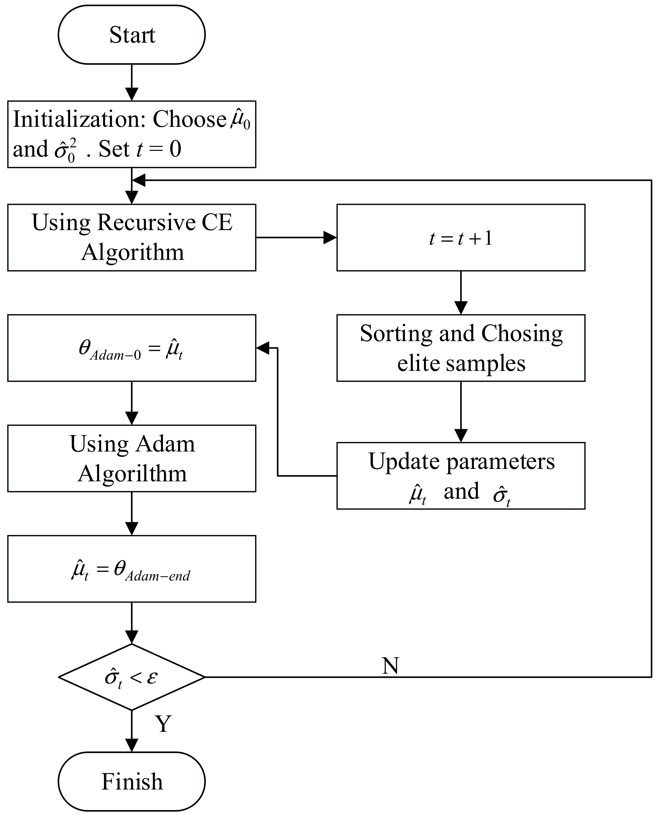
4. Cross-Entropy Adaptive Moment Estimation (CE-Adam) Algorithm

4.1. Recursive CE Algorithm

The CE algorithm has a good global optimization performance. However, the objective function values of all photons need to be calculated during each iteration, which leads to a large CPU time cost. A recursive CE algorithm is proposed to reduce the CPU time cost. The recursive CE algorithm divides all $N$ photons into subsets $[N_1,N_2,\dots ,N_n]$ according to the observation period and selects a subset in each iteration to calculate the objective function and update the parameters. In other words, the improvement of the recursive CE algorithm to the CE algorithm is that the objective function is changed to $S_t(•)$. The expression of $S_t(•)$ is:

$$\left\{\begin{array}{l}{S}_t(•)={\displaystyle \sum _{k=1}^{m_l}\log \mathit{\lambda }(t_k)},(N=[N_1,N_2,\dots ,N_n])\\ l=\mathrm{mod}(t,n)\end{array}\right.,$$

(17)

where $t$ is the number of iterations, $m_l$ is the capacity of $N_l$, and $N$ represents all photons, $N=[N_1,N_2,\dots ,N_n]$, $N_1,N_2,\dots ,N_n$ are the subsets of photons, and $N_l$ is the currently used subset.

The ${\tilde{\mu }}_k$ and ${\tilde{\sigma }}_k$ are calculated from Equation (14) and are used to update the ${\widehat{\mu }}_t$ and ${\widehat{\sigma }}_t$ by Equation (15).

4.2. Proposal of CE-Adam Algorithm

The recursive CE algorithm uses few photons in each iteration, which reduce the CPU time cost as well as the estimation accuracy of q and f. In order to overcome this disadvantage, the parameter updated by the recursive CE algorithm is used as the initial value of the Adam algorithm. Then, the final value of the Adam algorithm is used to update the distribution parameters of the recursive CE algorithm.

$$\left\{\begin{array}{l}{\theta }_{Adam-0}={\widehat{\mu }}_t\\ {\widehat{\mu }}_t={\theta }_{Adam-end}\end{array}\right.,$$

(18)

where ${\theta }_{Adam-0}$ and ${\theta }_{Adam-end}$ respectively represent the initial value and final value of Adam algorithm.

The above algorithm is called the CE-Adam algorithm, and its procedure can be described as follows. Firstly, the recursive CE algorithm is adopted. After each recursion, the Adam algorithm is applied with the updated parameter’s mean value as the initial value to obtain better than expected values of the parameters and update the distribution parameters of the recursive CE algorithm. The flow chart of the CE-Adam algorithm is shown in Figure 2.

5. Experiments

The simulation data of PSR B1821-24 and Crab pulsar and real data from NICER are used to verify the performance of the proposed CE-Adam algorithm. The algorithm is utilized to estimate q (initial phase) and f (frequency) in Equation (5). For simulation data, we define the evaluation criterion of the estimation performance is the RMS (root mean square) error of q. For the real data, the estimation performance is assessed by the error of estimated q relative to that obtained by the Global Positioning System (GPS). The computational cost is accessed by the CPU time cost. The computation environment contains Intel Core [email protected] (Intel, Santa Clara, CA, US), memory of 8G and python 3.8.

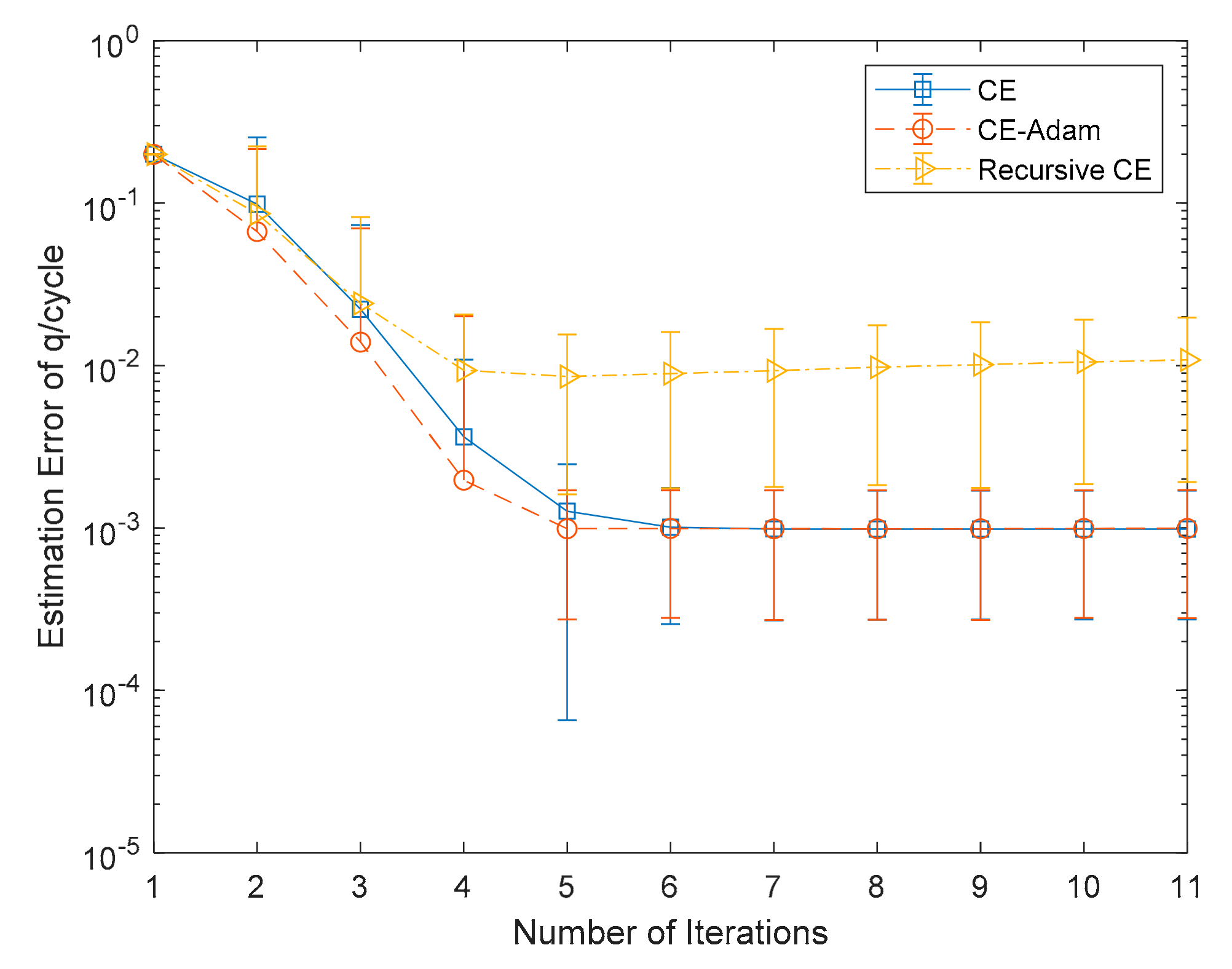
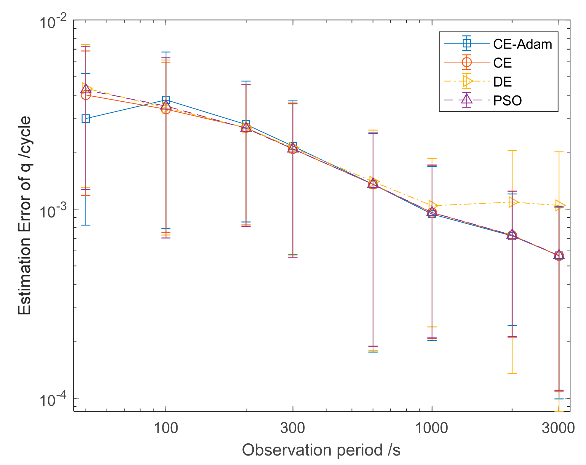
5.1. Experiments with Simulation Data

We chose the PSR B1821-24 pulsar, with the simulation parameters listed in

Table 1. Simulation parameters of PSR B1821-24 [15].

Parameters	Value
period/ms	3.05
$\alpha$/ph·s−1	1.93
$\beta$/ph·s−1	50

, as the observed pulsar [15], and the profile of it is given in Figure 3. The results are all calculated from 1000 Monte Carlo simulations.

Assuming that the observation period is 1000 s, the photon TOAs recorded by an orbiting spacecraft are simulated. The objective function for estimating q and f is Equation (5). We compare the estimation performance of the CE algorithm, recursive CE algorithm, and CE-Adam algorithm. The average estimation error of q from 1000 Monte Carlo simulations is shown in Figure 4. It can be seen that the estimation accuracy of q for the three algorithms increases with the iterations. The estimation error of q for the recursive CE algorithm is higher than the other algorithms. This is because that the recursive CE algorithm uses a few photons in each iteration, which reduces the estimation accuracy of q. The estimation result for the CE-Adam and the estimation result for the CE algorithm are close to each other. This is because the CE-Adam algorithm overcomes the problem of the recursive CE algorithm and greatly improves the estimation accuracy.

Figure 5 shows the estimation error of q obtained by the four algorithms. It can be seen that the estimation accuracy of q for the four algorithms increases with the increase of the observation period. When the observation period exceeds 1000 s, the estimation error of q of the DE algorithm is higher than PSO, CE and CE-Adam. The estimation error of q for PSO, CE and CE-Adam are close to each other.

Figure 6 shows the estimation error of f obtained with the four algorithms. It can be seen that the estimation accuracy of f for the four algorithms increases with the increase of the observation period. When the observation period exceeds 1000 s, the estimation error of f of the DE algorithm is higher than PSO, CE and CE-Adam. The estimation error of f for PSO, CE and CE-Adam are close to each other.

Table 2. Estimation error of q and f.

Observation Period/s	Estimation Error of q/1 × 10−3 Cycle				Estimation Error of f/1 × 10−6 HZ
	PSO	DE	CE	CE-Adam	PSO	DE	CE	CE-Adam
1000	0.958	1.04	0.957	0.94	1.7	1.90	1.69	1.68
2000	0.727	1.08	0.726	0.721	0.607	0.868	0.606	0.621
3000	0.567	1.04	0.565	0.567	0.319	0.585	0.318	0.325

shows the estimation error of q and f. It can be seen that the PSO, CE and CE-Adam perform a lower estimation error than DE. Since the pulse phase estimation is mainly focused on the pulse phase, the estimation of f will not be analyzed in the rest of this paper.

Figure 7 shows the CPU time cost by the four algorithms. Although the CPU time of CE-Adam algorithm is not the shortest when the observation period is less than 1000 s, its advantage gradually manifests when the observation period overtakes 1000 s. When the observation period reaches 3000 s, the CPU time cost of the CE-Adam algorithm is much lower than the others. For faint millisecond pulsar, in order to obtain an accurate estimation result, the observation period of more than 1000 s is needed. Therefore, compared with other algorithms, the algorithm proposed in this paper can reduce the CPU time cost while ensuring the accuracy of pulse phase estimation.

We assume that the observation period is 1000 s and compare the linearized method with the proposed method.

Table 3. Comparison of CPU time and estimation error of q.

Methods	Estimation Error of q/1 × 10−3 Cycle	CPU Time/s
Proposed method	0.95	26.4
Linearized method	1.2	8203.1

shows the estimation error of q and CPU time cost. It can be seen that the proposed method could obtain similar estimation error of q with shorter CPU time.

In addition, we investigated the estimation performance of the CE-Adam algorithm for Crab pulsar. Compared with PSR B1821-24, Crab pulsar has a lager flow rate, resulting in much higher CPU time cost.

Table 4. Simulation parameters of Crab pulsar [16].

Parameters	Value
period/ms	33.4
$\alpha$/ph·s−1	660
$\beta$/ph·s−1	13,860.2

shows the simulation parameters of the pulsar [16], and Figure 8 shows its profile. Assuming the observation period is 500 s, the photon TOAs recorded by the orbiting spacecraft are simulated. The objective function of estimating q and f is Equation (5). We compare the estimation performance of CE, DE, PSO, and the CE-Adam algorithm proposed in this paper.

Figure 9 shows the estimation error of q and CPU time for the four algorithms. It can be seen that the estimation accuracy of q for the four algorithms is not very different, but the CPU time cost of the CE-Adam algorithm is much lower than the other algorithms. Compared with the CE algorithm, the CPU time cost is about 1.5%; and compared with DE and PSO, the CPU time cost is about 2.8%.

5.2. Experiments with Real Data

NICER is the International Space Station (ISS) payload, which was launched in June 2017. It is mainly used to observe pulsars and neutron stars. NICER has a large effective area (>1800 cm²), wide band-pass (0.2–12.0 keV) and high time resolution (better than 300 ns) [30].

We use the real data of the Crab pulsar on 26 December 2018 (Obs (observation)_ID: 1013010147). The predicted orbit is used to correct the barycenter of photon TOAs, and the CE-Adam algorithm proposed in this paper is used for on-orbit pulse phase estimation. The parameters of the predicted orbit are listed in

Table 5. The estimated orbit parameters of the International Space Station (ISS).

Parameters	Value
Epoch	2018/12/26 00:31:03
Semi-major axis/km	677.0809
Eccentricity	0.0015
Inclination/°	51.6775
Ascending node ascension/°	142.3733
Perigee auxiliary angle/°	101.7365
True anomaly/°	161.7955

.

We selected eight groups of data with observation period longer than 2000 s, which are shown in

Table 6. The duration of real data.

Data	Duration
data 1	07:58:39–08:34:35
data 2	09:31:20–10:07:16
data 3	11:04:01–11:40:14
data 4	12:36:41–13:12:44
data 5	14:09:20–14:45:27
data 6	15:42:00–16:18:11
data 7	17:14:41–17:50:53
data 8	18:47:20–19:23:35

. The estimation performance was assessed by the error of estimated q relative to that obtained by GPS. Figure 10 shows CPU time and the estimation error of q for the CE-Adam algorithm. The average CPU time is 63.1 s, and the average error of estimation of q is 1.06 × 10⁻³.

Finding that the CPU time and q estimation error of dataset 1 are both exceptionally low, we used CE-Adam algorithm to process dataset 1 for 100 times. The results of estimation error of q and CPU time are shown in Figure 11. It can be seen that the estimation error of q and CPU time are uncertain. Most results of estimation error of q are about 1 × 10⁻³, and most results of CPU time are about 30 s. Although the RMS error of q is satisfactory, the uncertainty of the CE-Adam method could impact the estimation of q. Thus, further study is needed to overcome the uncertainty of the CE-Adam method.

6. Conclusions

In order to solve the problem in on-orbit pulse phase estimation that the CPU time cost increases sharply with the observation period, a pulse phase algorithm based on the CE-Adam algorithm, which has low CPU time cost and retains decent estimation accuracy, was proposed. Simulation results showed that the proposed algorithm had a lower CPU time cost than other algorithms. The on-orbit pulse phase estimation results obtained with real data of NICER showed that the algorithm proposed in this paper can quickly and accurately process the real data, which has practical engineering significance for pulsar navigation. In addition, we found that the uncertainty of the CE-Adam algorithm would impact the CPU time and accuracy of pulse phase estimation, which should be overcome in a further study.

References

1. Zheng, W.; Wang, Y. Introduction. In X-ray Pulsar–Based Navigation: Theory and Applications; Springer: Singapore, 2020; pp. 1–24. [Google Scholar] [CrossRef]
2. Chester, T.J.; Butman, S.A. Navigation Using X-Ray Pulsars. Telecommun. Data Acquis. Prog. Rep. 1981, 63, 22. [Google Scholar]
3. Mitchell, J.W.; Winternitz, L.B.; Hassouneh, M.A.; Price, S.R.; Semper, S.R.; Yu, W.H.; Ray, P.S.; Wolff, M.T.; Kerr, M.; Wood, K.S.; et al. Sextant x-ray pulsar navigation demonstration: Initial on-orbit results. In Proceedings of the 2018 SpaceOps Conference, Marseille, France, 28 May–1 June 2018. [Google Scholar]
4. Zheng, S.J.; Ge, M.Y.; Han, D.W. Test of pulsar navigation with POLAR on TG-2 spacelab. Sci. Sin. Phys. Mech. Astron. 2017, 47, 120–128. [Google Scholar] [CrossRef] [Green Version]
5. Zheng, S.J.; Zhang, S.N.; Lu, F.J.; Wang, W.B.; Gao, Y.; Li, T.P.; Song, L.M.; Ge, M.Y.; Han, D.W.; Chen, Y.; et al. In-orbit Demonstration of X-Ray Pulsar Navigation with the Insight-HXMT Satellite. Astrophys. J. Suppl. Ser. 2019, 244. [Google Scholar] [CrossRef] [Green Version]
6. Emadzadeh, A.A.; Speyer, J.L. X-Ray Pulsar-Based Relative Navigation using Epoch Folding. IEEE Trans. Aerosp. Electron. Syst. 2011, 47, 2317–2328. [Google Scholar] [CrossRef]
7. Emadzadeh, A.; Speyer, J.; Golshan, A. Asymptotically Efficient Estimation of Pulse Time Delay for X-Ray Pulsar Based Relative Navigation. In Proceedings of the AIAA Guidance, Navigation, and Control Conference, Chicago, IL, USA, 10–13 August 2009. [Google Scholar] [CrossRef] [Green Version]
8. Wu, Y.; Kang, Z.; Liu, J. A fast pulse time-delay estimation method for X-ray pulsars based on wavelet-bispectrum. J. Opt. 2020, 207, 1–11. [Google Scholar] [CrossRef]
9. Liu, L.; Liu, J.; Ning, X.; Kang, Z. Real-time and accurate pulsar time-of-arrival estimation using GA-optimized EMD-CS. J. Opt. 2021, 225, 1–11. [Google Scholar] [CrossRef]
10. Song, G.; Kang, Z.W. Fast Pulse Time Delay Estimation Algorithm Based on Variable Step Size Iteration. In Proceedings of the 4th International Conference on Information Science and Control Engineering (ICISCE), Changsha, China, 21–23 July 2017; pp. 1505–1509. [Google Scholar] [CrossRef]
11. Golshan, A.R.; Sheikh, S.I. On Pulse Phase Estimation and Tracking of Variable Celestial X-Ray Sources. In Proceedings of the 63rd Annual Meeting of the Institute of Navigation, Cambridge, MA, USA, 23–25 April 2007. [Google Scholar]
12. Huang, L.; Liang, B.; Zhang, T. Pulse phase and doppler frequency estimation of X-ray pulsars under conditions of spacecraft and binary motion and its application in navigation. Sci. China-Phys. Mech. Astron. 2013, 56, 848–858. [Google Scholar] [CrossRef]
13. Anderson, K.D.; Pines, D.J.; Sheikh, S.I. Validation of Pulsar Phase Tracking for Spacecraft Navigation. J. Guid. Control. Dyn. 2015, 38, 1885–1897. [Google Scholar] [CrossRef]
14. Winternitz, L.M.B.; Hassouneh, M.A.; Mitchell, J.W.; Valdez, J.E.; Price, S.R.; Semper, S.R.; Yu, W.H.; Ray, P.S.; Wood, K.S.; Arzoumanian, Z.; et al. X-ray Pulsar Navigation Algorithms and Testbed for SEXTANT. In Proceedings of the 2015 IEEE Aerospace Conference, Big Sky, MT, USA, 7–14 March 2015. [Google Scholar]
15. Wang, Y.; Zheng, W. Pulse Phase Estimation of X-ray Pulsar with the Aid of Vehicle Orbital Dynamics. J. Navig. 2016, 69, 414–432. [Google Scholar] [CrossRef] [Green Version]
16. Wang, Y.; Zheng, W. Pulse Phase and Doppler Frequency Estimation for XNAV Using On-orbit Epoch Folding. IEEE Trans. Aerosp. Electron. Syst. 2016, 52, 2210–2219. [Google Scholar] [CrossRef]
17. Kolda, T.G.; Lewis, R.M.; Torczon, V. Optimization by direct search: New perspectives on some classical and modern methods. SIAM Rev. 2003, 45, 385–482. [Google Scholar] [CrossRef]
18. Xue, M.; Li, X.; Fu, L.; Fang, H.; Sun, H.; Shen, L. X-ray pulsar-based navigation using pulse phase and Doppler frequency measurements. Sci. China Inf. Sci. 2015, 58, 1–14. [Google Scholar] [CrossRef] [Green Version]
19. Chen, Y.; Cui, W.; Li, W.; Wang, J.; Xu, Y.; Lu, F.; Wang, Y.; Chen, T.; Han, D.; Hu, W.; et al. The Low Energy X-ray telescope (LE) onboard the Insight-HXMT astronomy satellite. Sci. China Phys., Mech. Astron. 2020, 63, 249–505. [Google Scholar] [CrossRef] [Green Version]
20. Bogdanov, S.; Guillot, S.; Ray, P.S.; Wolff, M.T.; Chakrabarty, D.; Ho, W.C.G.; Kerr, M.; Lamb, F.K.; Lommen, A.; Ludlam, R.M.; et al. Constraining the Neutron Star Mass–Radius Relation and Dense Matter Equation of State with NICER. I. Astrophys. J. 2019, 887, L25. [Google Scholar] [CrossRef] [Green Version]
21. Emadzadeh, A.A.; Speyer, J.L. Pulse Delay Estimation. In Navigation in Space by X-ray Pulsars; Springer: New York, NY, USA, 2011. [Google Scholar] [CrossRef]
22. De Boer, P.T.; Kroese, D.P.; Mannor, S.; Rubinstein, R.Y. A tutorial on the cross-entropy method. Ann. Oper. Res. 2005, 134, 19–67. [Google Scholar] [CrossRef]
23. Kroese, D.P.; Porotsky, S.; Rubinstein, R.Y. The cross-entropy method for continuous multi-extremal optimization. Methodol. Comput. Appl. Probab. 2006, 8, 383–407. [Google Scholar] [CrossRef]
24. Zhao, D.; Huang, C.; Tang, Q. CEGA: Research on Improved Multi-objective CE Optimization Algorithm. In Proceedings of the 37th Chinese Control Conference, Wuhan, China, 25–27 July 2018; pp. 2463–2467. [Google Scholar]
25. Kingma, D.; Ba, J. Adam: A Method for Stochastic Optimization. 3rd International Conference for Learning Representations, San Diego, CA, USA, 7–9 May 2015; pp. 1–15. [Google Scholar]
26. Zhou, J.; Wang, H.D.; Wei, J.L.; Liu, L.; Huang, X.C.; Gao, S.C.; Liu, W.P.; Li, J.P.; Yu, C.Y.; Li, Z.H. Adaptive moment estimation for polynomial nonlinear equalizer in PAM8-based optical interconnects. Opt. Express 2019, 27, 32210–32216. [Google Scholar] [CrossRef] [PubMed]
27. Storn, R.; Price, K. Differential Evolution—A Simple and Efficient Heuristic for global Optimization over Continuous Spaces. J. Glob. Optim. 1997, 11, 341–359. [Google Scholar] [CrossRef]
28. Kennedy, J. Particle Swarm Optimization. In Encyclopedia of Machine Learning; Sammut, C., Webb, G.I., Eds.; Springer: Boston, MA, USA, 2010; pp. 760–766. [Google Scholar] [CrossRef]
29. Emadzadeh, A.A.; Speyer, J.L. On Modeling and Pulse Phase Estimation of X-Ray Pulsars. IEEE Trans. Signal Process. 2010, 58, 4484–4495. [Google Scholar] [CrossRef]
30. Gendreau, K.; Arzoumanian, Z.; Adkins, P.; Albert, C.; Anders, J.; Aylward, A.; Baker, C.; Balsamo, E.; Bamford, W.; Benegalrao, S.; et al. The Neutron star Interior Composition Explorer (NICER): Design and Development; SPIE: Bellingham, WA, USA, 2016; Volume 9905. [Google Scholar]
Figure 1. Extremal distribution of the objective function.
Aerospace 08 00095 g001
Figure 2. Flow chart of the cross-entropy adaptive moment estimation (CE-Adam) algorithm.
Aerospace 08 00095 g002
Figure 3. Profile of PSR B1821-24.
Aerospace 08 00095 g003
Figure 4. Monte Carlo simulation results.
Aerospace 08 00095 g004
Figure 5. Estimation error of q for cross-entropy (CE), differential evolution (DE), particle swarm optimization (PSO) and CE-Adam algorithm.
Aerospace 08 00095 g005
Figure 6. Estimation error of f for CE, DE, PSO and CE-Adam algorithm.
Aerospace 08 00095 g006
Figure 7. Comparison of central processing unit (CPU) time.
Aerospace 08 00095 g007
Figure 8. Profile of Crab pulsar.
Aerospace 08 00095 g008
Figure 9. Comparison of CPU time and estimation error of q.
Aerospace 08 00095 g009
Figure 10. Crab pulsar real data results.
Aerospace 08 00095 g010
Figure 11. Crab pulsar real data results.
Aerospace 08 00095 g011