A Numerical and Experimental Investigation of the Convective Heat Transfer on a Small Helicopter Rotor Test Setup

Abstract

In-flight icing affects helicopter performance, limits its operations, and reduces safety. The convective heat transfer is an important parameter in numerical icing simulations and state-of-the-art icing/de-icing codes utilize important computing resources when calculating it. The BEMT–RHT and UVLM–RHT offer low- and medium-fidelity approaches to estimate the rotor heat transfer (RHT). They are based on a coupling between Blade element momentum theory (BEMT) or unsteady vortex lattice method (UVLM), and a CFD-determined heat transfer correlation. The latter relates the Frossling number (Fr) to the Reynolds number (Re) and effective angle of attack (α_Eff). In a series of experiments carried out at the Anti-icing Materials International Laboratory (AMIL), this paper serves as a proof of concept of the proposed correlations. The objective is to propose correlations for the experimentally measured rotor heat transfer data. Specifically, the Fr_x is correlated with the Re and α_Eff in a similar form as the proposed CFD-based correlations. A fixed-wing setup is first used as a preliminary step to verify the heat transfer measurements of the icing wind tunnel (IWT). Tests are conducted at α = 0°, for a range of 4.76 × 10⁵ ≤ Re ≤ 1.36 × 10⁶ and at 10 non-dimensional surface wrap locations − 0.62 ≤ (S/c) ≤ + 0.87. Later, a rotor setup is used to build the novel heat transfer correlation, tests are conducted at two pitch angles ((θ) = 0° and 6°) for a range of rotor speeds (500 RPM ≤ (Ω) ≤ 1500 RPM), three different radial positions ((r/R) = 0.6, 0.75 and 0.95), and 0 ≤ S/c ≤ + 0.58. Results indicate that the fixed-wing Fr_x at the stagnation point was in the range of literature experimental data, and within 8% of fully turbulent CFD simulations. The Fr_Avg also agrees with CFD predictions, with an average discrepancy of 1.4%. For the rotor, the Ω caused a similar increase of Fr_x for the tests at θ = 0° and those at θ = 6°. Moreover, the Fr_x behavior changed significantly with r/R, suggesting the α_Eff had a significant effect on the Fr_x. Finally, the rotor data are first correlated with Re^m (at each S/c) for θ = 0° to establish the correlation parameters, and a term for the α_Eff is then added to also account for the tests at θ = 6°. The correlations fit the data with an error between 2.1% and 14%, thus justifying the use of a coupled approach for the BEMT–RHT and UVLM–RHT.

1. Introduction

Aircraft are vulnerable to in-flight and pre-flight icing that limit their operations. Indeed, icing causes flight delays during ground de-icing interventions, flight cancellations because of forecast or actual in-cloud icing [1]. During flight, liquid water impinging on an aircraft will freeze to its surfaces even when the outside air temperature (OAT) is above 0 °C [2]. According to [2,3], pilot-reduced visibility is a direct result of in-flight ice accumulation on windscreen and instrument ports. In addition, added weight on the airframe reduces the load capacity and increases fuel consumption. In the case of a helicopter, the most adverse effect of blade contamination comes from the aerodynamics of the iced main rotor blade, which will result in reduced lift and an increase in drag [3]. A subsequent loss of thrust and possible flow separation generated by the main and tail rotors may lead to the total loss of control. Severe vibrations may also be induced by the shedding of ice that can force emergency landings. Although the primary concern is with the main rotor, the protection of the tail rotor requires similar considerations.

Calculating the convective heat transfer on airfoils is an important first step in the operation of icing codes. According to a study on the assessment of thermodynamic models for ice accretion [4], heat transfer by convection is one of the most important terms in the heat balance for a successful icing/de-icing simulation of aircraft. In the literature, the convective heat transfer from standard geometrical configurations such as flat plates, cylinders, and spheres has been studied and reported extensively. Correlations were developed for the Nusselt (Nu) or (Fr) Frossling numbers based on a product of the Reynolds (Re) and Prandtl (Pr) numbers, in the form of Equation (1) [5,6], where Fr = Nu × Re^−0.5. These correlations are associated with parameters (A) and (m) that differ if the flow is laminar or turbulent, or if the thermal boundary conditions (TBC) are either a constant surface temperature (T_S) or a constant surface heat flux (Q_S) [6]. Of the most recent studies, a correlation is proposed even for the Nu in the transition region of the flat plate [7].

$$Fr=A\times {\mathrm{Re}}^m\times {\mathrm{Pr}}^{1/3}$$

(1)

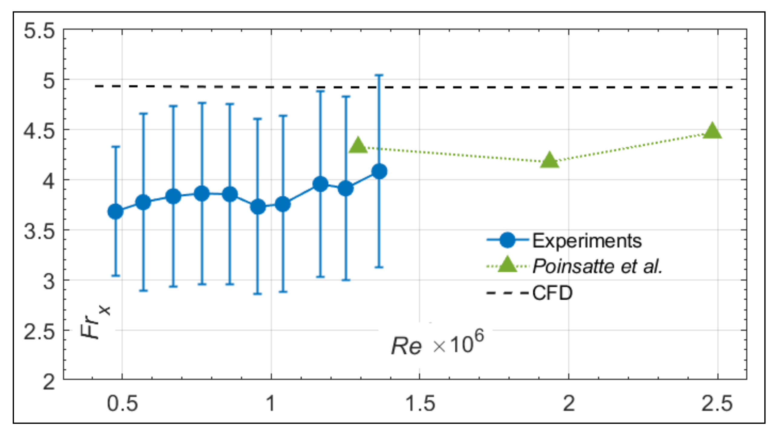
The case of airfoil heat transfer is more complex, given the thicknesses involved and the effects of angles of attack (α). Yet, the literature indicates that for fixed-wing airfoils, the convective heat transfer has been thoroughly studied. The work of Poinsatte et al. [8] provided a comprehensive analysis of airfoil heat transfer when they quantified the heat transfer on the leading edge (LE) of a smooth and roughened NACA 0012. Their data were gathered from in-flight measurements of the NASA Lewis Twin Otter (NASA Lewis Research Center Cleveland, OH, USA) icing research aircraft and experiments in the Icing Research Tunnel (IRT). The experimented airfoil’s LE up was maintained on a constant surface temperature using embedded heating gauges located between −3.6% and 9.5% of the dimensionless wrap distance S/c. A total of 46 tests were carried out for −6° ≤ α ≤ 8° and 1.2 × 10⁶ ≤ Re ≤ 2.4 × 10⁶. The measured heat transfer on the airfoil was compared to the results of the flat plate under laminar and turbulent flow conditions and the cylinder correlations. For the smooth surface tests, their work affirmed the use of the Fr and showed that the behavior of heat transfer in the laminar flow portion was similar to the behavior seen on the cylinder and the flat plate for the same flow conditions. They used Equation (1) to successfully correlate the Fr_x at each S/c with Re and found that on the stagnation point and near the LE, the correlations show values of m = 0. The Fr curves collapse into one in the laminar flow region making the Fr independent of Re.

A set of experiments between 2006 and 2008 by Wang et al. [9,10,11,12] measured the average Nusselt number (Nu_Avg) on the surface of a hollowed NACA 63-421. The experimented airfoil was equipped with heating strips installed on the inner edges of the airfoil. The heaters were set to provide a constant heat flow of 500 W that was transferred to the airflow by conduction through the airfoil material. A total of 25 thermocouples were distributed across the chord on the exterior and interior surfaces of the airfoil to measure the temperature differences. They also correlated their data, in terms of the Nu_Avg, based on Equation (1). Their main contribution was in the expansion of the A term in Equation (1) to account for the α and liquid water content (LWC). Correlations were formed for dry air at α = 0° [9] and 0° ≤ α ≤ 25° [10], in addition to 0 ≤ LWC ≤ 4.98 g/m³ at α = 0° [11] and 0° ≤ α ≤ 25° [12].

The static pressure and heat transfer rates were measured by Li et al. on the surface of a thick BO28 airfoil at locations covering 90% of both the top and bottom surfaces for −8.5° ≤ α ≤ 19.5° and Re = 2.5 × 10⁵, 5.82 × 10⁵ and 1.085 × 10⁶ [13]. The airfoil had 23 embedded heating tiles that were heated to a specified constant temperature. They paid close attention to the effect of flow transition on the increased heat transfer between the laminar and turbulent flow regions by calculating the Fr on various chord locations. Their tests again showed independence of the Fr on the Re in the laminar flow region on the airfoil, confirming the results of [8]. When the Re was fixed and the α was increased, flow transition on the suction side of the airfoil moved closer to the LE, and an abrupt increase of heat transfer was detected. On the pressure side, the transition point was pushed towards the trailing edge and a similar abrupt increase of heat transfer was also observed. When the α was fixed and the Re was increased, the increase of heat transfer due to flow transition was pushed closer to LE on both surfaces of the airfoil. For all tests, high Fr values were observed on the stagnation point however, the highest Fr values were actually observed on locations where the flow transitioned from laminar to turbulent. The abrupt increase of Fr at the transition point was followed by a less severe yet rapid decrease of Fr values downstream towards the trailing edge.

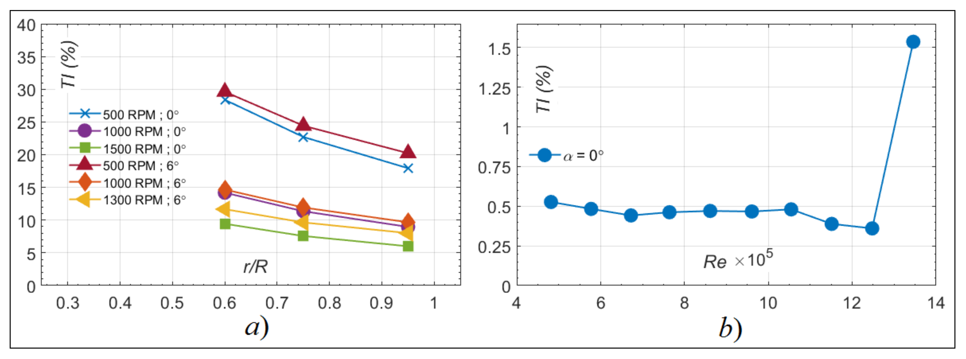
Many factors add to the complexity of rotor heat transfer estimation compared to fixed-wing platforms. For instance, the rotation of the blades causes the blade local velocity (and associated Re) to increase from root to tip. Moreover, tip vortices are formed when the pitch angle is varied, creating a range of α_Eff across the blade radius. To further complicate the problem, the interaction of a freestream velocity (V_∞) with the rotating blades (as in the case of forward flight) produces advancing and retreating regions in the plane of rotation. The blade local velocity, therefore, experiences fluctuations that in turn generate high levels of turbulence intensity (TI). Turbulent heat transfer augmentation is a direct result of the TI that, according to [14], affects the stagnation, laminar, and turbulent regions of flows on airfoils.

To the best of the authors’ knowledge, there are no previous experimental attempts to correlate heat transfer data measured on the surface of a small helicopter tail rotor. Although extensive experimental efforts have been made on rotor icing in the past [15,16,17,18,19], the literature still lacks a correlation that considers both radial and chordwise variations of the Fr_x. Moreover, a recent study by Aubert [20] also found that the entire rotor simulation process from ice accretion to impact to shedding needs refinement. He reviewed previous icing rotor studies and concluded that the ice structure formed on rotor blades is not fully understood and that the type of accreted ice from the blade root to tip and the mechanical properties can vary. He also concluded that most numerical solvers, including their heat transfer calculation schemes, need enhancement for better icing and de-icing predictions.

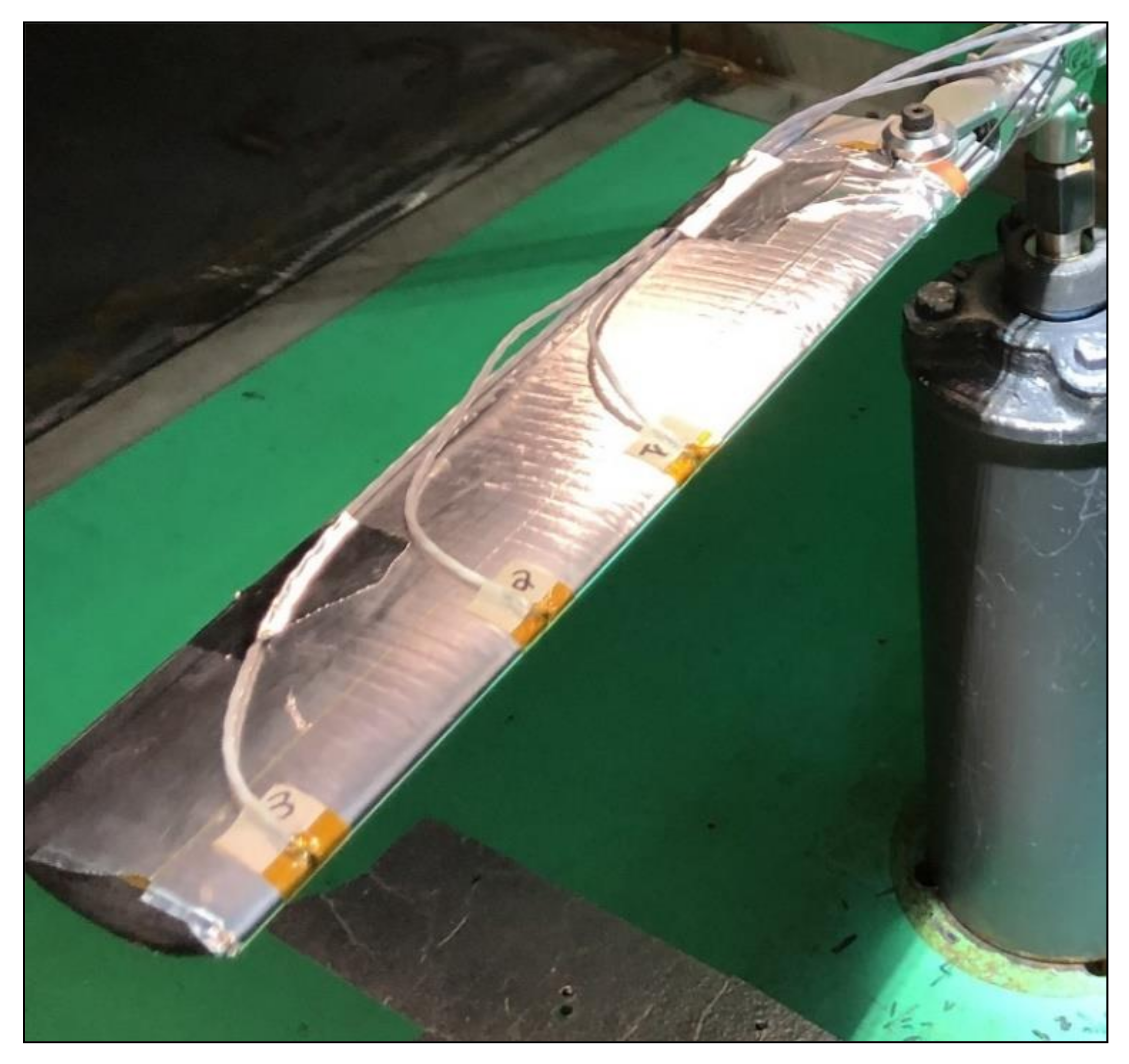
In an earlier publication, Samad et al. [21] proposed the use of low- and medium-fidelity numerical tools for heat transfer calculation of a small helicopter tail rotor. The tools are known as the BEMT–RHT and UVLM–RHT. They implement the Blade element momentum theory (BEMT) and the unsteady vortex lattice method (UVLM), on one hand, and a CFD-determined heat transfer correlation for an airfoil under fully turbulent flow conditions, on the other. The correlation is an expanded version of Equation (1) and describes the airfoil Fr_Avg in the form of Equation (2). The coupling leads to an increase of fidelity, maintains the relatively computationally inexpensive solution, and provides an added layer of heat transfer prediction.

$$\begin{array}{c}F{r}_{Avg}=0.023\times \left(1-0.389\times {\alpha }_{Eff}-0.678\times {\alpha }_{Eff}^2\right){\mathrm{Re}}^{0.330}{\mathrm{Pr}}^{1/3}\hspace{1em}\left\{\begin{array}{c}2\times {10}^5\le \mathrm{Re}\le 3\times {10}^6\\ 0^{\circ }\le \alpha \le {30}^{\circ }\end{array}\right.\end{array}$$

(2)

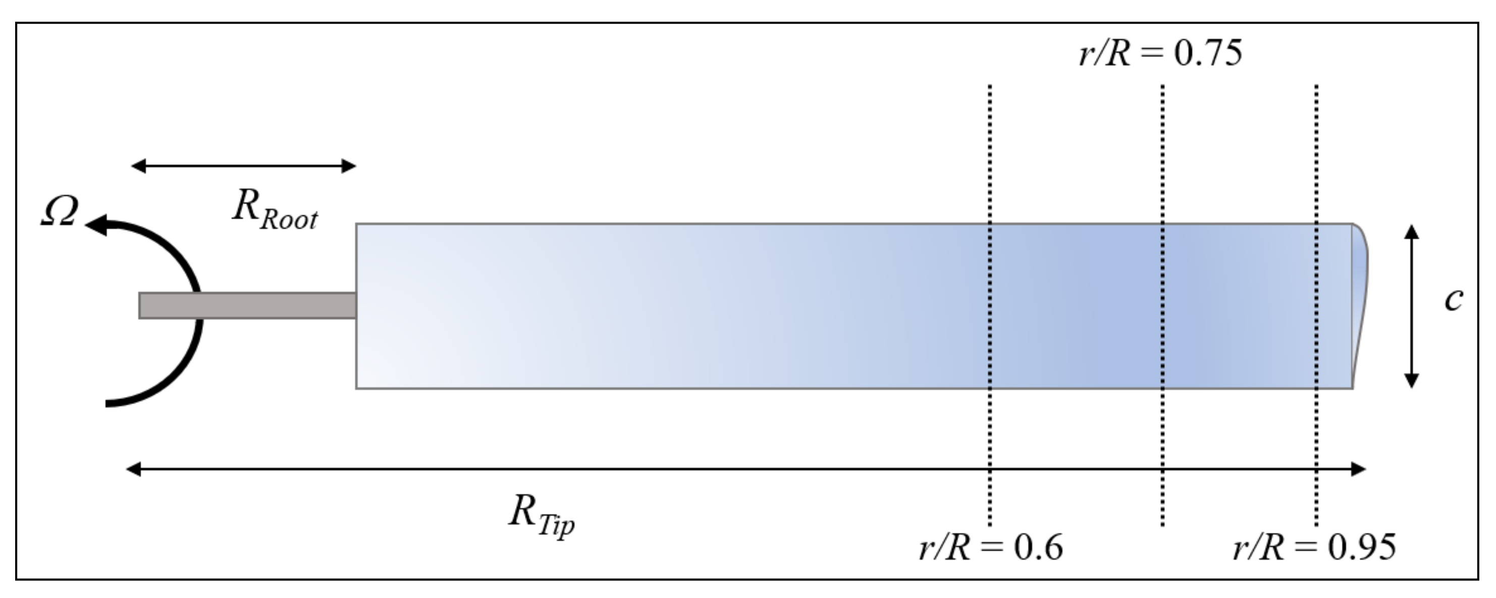
The objective of this paper is to correlate the measured Fr_x on the rotor surface with Re and α_Eff in a similar way as Equation (2). If the objective is met, it is believed the heat transfer prediction methodology of the BEMT–RHT and UVLM–RHT could be validated.

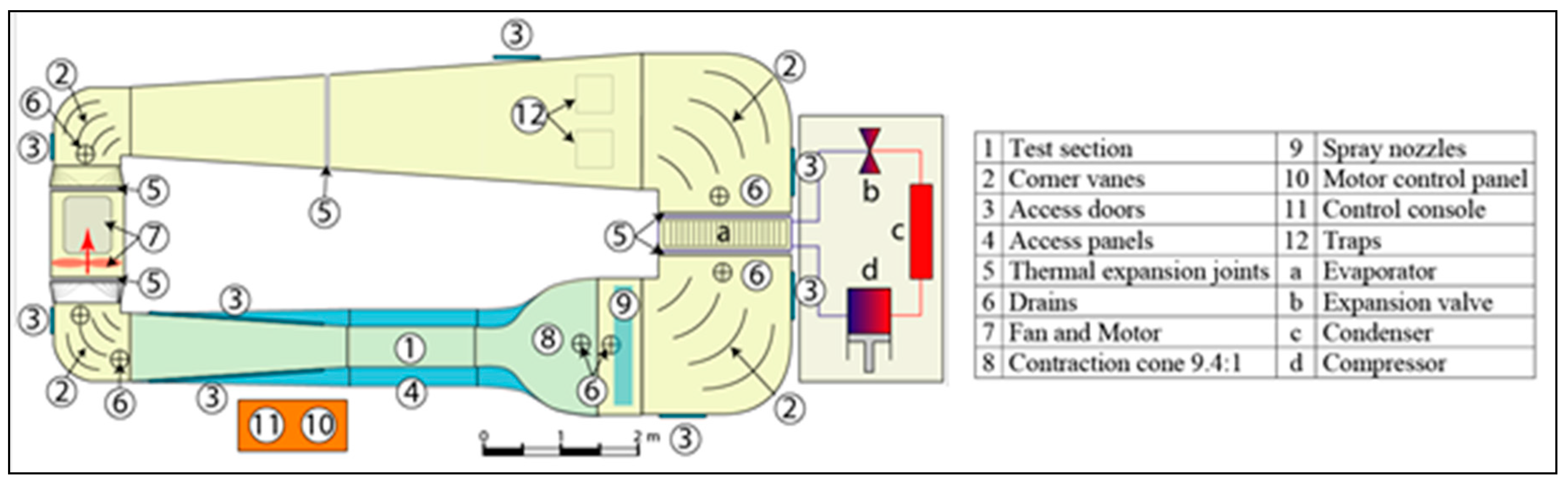
In the following sections, a description of the icing wind tunnel (IWT) is presented first. This is followed by a description of the fixed-wing and rotor experimental setups, along with the details of design and construction. Next, the methodology followed to calculate the convective heat transfer is outlined, together with the procedure to estimate heat losses, calculate the TI, and the experimental error. The test plan is laid out, and the procedure is followed for data acquisition and averaging. In the Results section, the calculated TI and the estimated heat losses due to radiation and conduction are discussed first. Heat transfer measurements are reported in terms of the Fr_x at the specified measurement locations and the Fr_Avg. The fixed-wing measurements are used for verification, where the stagnation point data are compared to previous experimental data from the literature and to CFD predictions. Finally, the rotor Fr_x data at each S/c and θ are then correlated with Re and α_Eff, in a similar form as Equation (2).

2. Materials and Methods

2.1. Icing Wind Tunnel (IWT)

The fixed-wing and rotor experimental setups were designed for testing in a refrigerated wind tunnel at Anti-icing Materials International Laboratory (AMIL), located in Chicoutimi, Québec, Canada. The wind tunnel meets the conditions of the SAE Aerospace Recommended Practice (Society of Automotive Engineers, Warrendale, PA, USA) for icing wind tunnel ARP5905 [22] and Aerospace Information Report for droplet sizing AIR4906 [23]. Figure 1 shows a general view of the IWT initially described in [24]. The tunnel is a closed recirculating type that cools the flow immediately downstream of the test section. The refrigeration system capacity can vary the total air temperature between −48°C and 22°C. This is achieved by passing air through a heat exchanger of 1.6 m by 1.6 m, powered by a compressor and a glycol pump.

The IWT is a closed-loop, low-speed refrigerated wind tunnel able to operate at sub-zero temperatures at sea level pressure and has two test sections. The smaller test section, which was used for the fixed-wing experiments, is 0.5 m wide by 0.6 m high and tests can be run at airspeeds up to 110 m/s at room temperature. The larger test section, which was used for the rotor experiments, is 0.91 m wide by 0.76 m high and tests can be run at airspeeds up to 50 m/s at room temperature. The IWT test section’s airspeed is controlled by a computer via a control program and data acquisition card. The test section’s airspeed is calculated with the Bernoulli equation and given by Equation (3).

$$V_{Test\mathit{Section}}=\sqrt{2{\left(1-\frac{A_{Test\mathit{Section}}^2}{A_{Ramp\mathit{Section}}^2}\right)}^{-1}\frac{p_{Ramp\mathit{Section}}-p_{Test\mathit{Section}}}{{\rho }_{air}}}$$

(3)

2.2. Fixed-Wing Experiments

2.2.1. Convection Tests

The base aluminum airfoil consisted of a NACA 0012, as shown in Figure 2, with a span (b) = 30.5 cm (12″) and a chord (c) = 20.3 cm (8″). The airfoil was covered with 15 strip heating elements that provided a constant heat flux once activated. The size of each heating element was 2.5 cm × 30.5 cm (1″ × 12″) with a maximum power of 300 W. Two external DC power sources were connected to the heating elements. The first supplied heaters 1 to 8 (LE and suction side) with 62 W and the second power source supplied heaters 9 to 15 (pressure side) with 55 W. This way, a uniform heat flux of Q_Elec ≈ 10³ W/m² was obtained across the surface. With the imposed Q_Elec, the temperature gradient between the RTDs (Resistance Temperature Detectors) and air was greater than 3 °C for all tests.

Wiring limited the number of possible calibrated RTDs to 10. The RTDs were distributed across the chord of the airfoil to measure the temperatures at these different locations via an RTD recorder at a rate of one recording per second. The locations of the RTDs are shown in Figure 3 with the gray cylinder symbol. The strip heating elements are represented by the divided zones on the skin of the airfoil in Figure 3 and are numbered in Roman numerals I to XV.

Table 1. Chordwise position of fixed-wing outer RTDs.

RTD#	10	9	8	7	1	2	3	4	5	6
S/c	−0.625	–0.374	–0.248	–0.124	0	0.124	0.248	0.374	0.625	0.874
x/c	–0.608	–0.358	–0.232	–0.108	0	0.108	0.232	0.358	0.608	0.856

presents the position of the RTDs in terms of the non-dimensional curve length as a fraction to the chord S/c. The RTDs were installed at the middle of the heating elements in the chordwise direction and at the half-span.

Table 2. Fixed-wing test plan with respect to V_∞, α, and Re.

≈ Rec	V∞ (m/s)	Test ID# α = 0°; T∞ ≈ 273.15 K	V∞ (m/s)	Test ID# α = 0°;T∞ ≈ 263.15 K
5 × 105	31.56	1	29.49	11
6 × 105	37.87	2	35.39	12
7 × 105	44.18	3	41.29	13
8 × 105	50.49	4	47.9	14
9 × 105	56.81	5	53.09	15
1 × 106	63.12	6	58.99	16
1.1 × 106	69.43	7	64.88	17
1.2 × 106	75.74	8	70.78	18
1.3 × 106	82.05	9	76.68	19
1.4 × 106	89.4	10	88.01	20

shows the details for all tests conducted on the profile. Each test had a unique ID# that corresponded to a specific freestream temperature (T_∝), velocity (V_∝), and α. The table also shows the approximate Re for each test based on the T_∝ and V_∝ (the actual values will be presented with the results). The range of Mach number used was 0.09 ≤ (Ma) ≤ 0.27. In total, 10 tests were conducted at T_∝ ≈ 273.15 K for α = 0°, 10 more tests were conducted at T_∝ ≈ 263.15 K and α = 0° for the purpose of estimating the randomness error.

To avoid tunnel heating or temperature deviations, the tunnel compressor was set to a much lower operating temperature to try to maintain the circulating air at the desired T_∝. The test durations at Re ≥ 9 × 10⁵ were also shortened to 300 s, following a review of results because the Fr usually reached their steady-state values at that time.

2.2.2. Conduction Tests

To estimate the conduction in the airfoil skin, another set of tests was conducted in which four RTDs were installed inside the airfoil skin at mid-span, matching positions with four other RTDs on the outer surface. They were placed in the areas judged most critical of the airfoil as shown in Figure 4. RTD 2 was positioned on the inner nose of the LE, RTD 3 was at S/c = 0.124 of the bottom side of the airfoil, and RTDs 1 and 4 were placed at S/c = 0.312 on either side of the airfoil, as described in

Table 3. Chordwise position of fixed-wing inner RTDs.

RTD	Ti,1 & To,1	Ti,2 & To,2	Ti,3 & To,3	Ti,4 & To,4
S/c	0.312	0	−0.124	−0.312
x/c	0.296	0	−0.108	−0.296

. The inner RTDs were placed perpendicularly adjacent to the other RTDs at the outer airfoil surface. T_i,1 was directly below T_0,1, T_i,2 was directly on the right side of T_0,2, T_i,3 was directly above T_0,3, and T_i,4 was directly above T_0,4. The assumption was that the conductive heat transfer will be most significant in the perpendicular direction compared to the lateral due to the great scale between the airfoil chord c and its thickness (δ), similar to the assumption of [10].

Table 4. Fixed-wing test plan with respect to V_∞, α, and Re.

≈ Rec	V∞ (m/s)	Test ID# α = 0°; T∞ ≈ 273.15 K
1 × 105	6.31	1
2 × 105	12.62	2
3 × 105	18.93	3
4 × 105	25.25	4
5 × 105	31.56	5
6 × 105	37.87	6

shows the details for all the conduction tests performed on the profile. Each test had a unique ID# that corresponded to a specific V_∝. The table also shows the approximate Re for each test based on the T_∝ and V_∝. In total, six tests were performed at T_∝ ≈ 273.15 K for α = 0° with a similar heating power as the convection tests (Q_Elec ≈ 10³ W/m²).

2.3. Rotor Experiments

The powered spinning rotor blade (P–SRB) setup was designed by modifying the spinning rotor blade (SRB) setup previously developed at AMIL [24]. The original setup is composed of two blades in horizontal rotation connected to a hub and driven by a motor and a power shaft transmission. The SRB diameter, which is restricted by the AMIL IWT test section, is 0.780 m.

2.3.1. Powered Spinning Rotor Blade (P–SRB)

In the P–SRB, modifications were brought to the setup to bring electrical power to the spinning blades with the help of a IEC-FR-LC-10 slip ring by IEC Corporation (Austin, TX, USA) [25]. The hub was connected to a 3600 RPM 10 hp motor by a 2.54 cm (1″) diameter power steel shaft connected to a 10 hp drive. To safely operate the P–SRB in the IWT, the test section windows are made of polycarbonate thermoplastic resin (Lexan), which has high impact resistance. The motor-generator was computer-controlled and set at a constant rotor speed. The spinning rotor blade angular speed is measured by an optical encoder. The hub was a homemade modification of a G4 raptor hub with a diameter of 200 mm. This hub has no stabilizers. The blade pitch angle can be set at 0 and 6°. Power to supply the heating elements was generated by an Elektro-Automatik (Viersen, Germany) EA-PS3150-04B laboratory power supply.

The rotor blades were untwisted extruded 6063-T6 aluminum NACA 0012 profiles with a mill finish used for tail rotor blades of small helicopters. The extruded rotor blade could easily be modified to suit the test requirements and was free of rivets or other imperfections. The blade characteristics are presented in

Table 5. Powered spinning rotor blade (P–RSB) geometric characteristics.

Blade Root Distance	Blade Span (Radius)	Blade Chord
75.0 mm	390.0 mm	69.8 mm
Blade Twist	Number of Blades	Material
0°	2	6063-T6 Al

. The span is the rotor blade length from the rotation point to the blade tip. The length is the blade length from the hand attachment to the blade tip.

2.3.2. Rotor Construction

The rotor airfoil section had a NACA 0012 profile made of aluminum. Each blade was covered with one strip heating element that provided a constant heat flux once activated. This replicates the operation of a tail rotor in anti-icing, where ice accretion is eliminated by the heat supplied. The size of each heating element was 12.7 cm × 30.48 cm with a maximum power of 300 W. Preparatory rotor tests showed that a Q_Elec similar to that of the fixed-wing tests would produce fluctuations in the temperature gradient between air and RTDs. The Q_Elec was increased until a value of Q_Elec ≈ 6 × 10³ W/m² showed the least fluctuations. To achieve that value, the supplied voltage was set at (U_V) = 100 V and the current at (I_A) = 2.31 A. The total electric heating power was then 231 W, or a heating density of around Q_Elec ≈ 5.97 × 10³ W/m². The temperature in the tunnel was maintained at (T_∝) ≈ 248.15 K. The freestream air velocity was (V_∝) = 5.00 m/s, being the minimum possible needed the maintain the T_∝ by the IWT.

Figure 5 shows a close-up on the blade with three placed RTDs. To help minimize losses, the aluminum tape was used to cover the heating element and to try to provide an even distribution of heat. At each test and as shown in the figure, three calibrated RTDs were distributed across the radius of the experimented blade to measure the temperatures at these different locations via an RTD recorder at a rate of five recordings per second. The blade vibration rates were observed by an in-house software (Richvale Whittier, CA, USA) to to guarantee stable rotation.

Table 6. Details of test environment and heaters.

Rotor Speed	Airspeed V∞	Air Temperature T∞	Blade Pitch θ
500 < Ω < 1500	5.00 m/s	248.15 K	0°–6°
Heater Area	Heating Power	Heating Density	Heating Elements
387.1 cm2 (60 in2)	231 W	5.97 × 103 W/m2	1 per Blade

provides the details of the test environment and the heating element size and specifications. Two pitch angles were tested. The first is θ = 0° and is later used to obtain the correlation parameters A and m since the α_Eff = 0°. The second pitch angle is θ = 6° and is later used to fit the correlation based on a variation with α_Eff because the positive pitch creates a varying α_Eff on the blade.

For safety reasons, the maximum rotor speed was limited to 1500 RPM. Keeping that in mind and to provide the widest range of Re possible, three different rotor speeds were used Ω = 500 RPM, 1000 RPM, and 1500 RPM at θ = 0°. In contrast, at θ = 6° and due to vibrations in the system, the highest Ω was 1300 RPM; therefore, the three different rotor speeds used were Ω = 500 RPM, 1000 RPM, and 1300 RPM.

To obtain measurements at different radial positions of the blade, three RTDs were fitted on the blade. Only three RTDs could be fitted due to wiring limitations by the slip ring. Figure 6 shows a sketch of the experimented blade with the radial locations of interest. Furthermore, to increase the range of Re, the RTDs were placed at r/R = 0.6, 0.75, and 0.95, where (r/R) is the ratio of local RTD radius to blade tip.

To obtain measurements at different chordwise positions of the rotor, a specific non-dimensional chord distance (x/c) was set (for example, x/c = 0 or x/c = 1/7, etc.) for each test. This configuration was used to do tests at the three different rotor speeds before the x/c was changed. Figure 7 shows a sketch of the airfoil section with the chordwise positions x/c of interest.

It should be noted that at any test, only a specific x/c was tested at the same time. The RTDs were first placed at x/c = 0 and three tests were carried out for the three Ω. The RTDs were then taken off and placed on the next x/c at the same r/R, and the three rotor speeds were tested again sequentially. This was repeated until all x/c positions were tested.

Table 7. Rotor test plan at V_∝ = 5.00 m/s and θ = 0°.

x/c	S/c	500 RPM	1000 RPM	1500 RPM	r/R
0	0	1	2	3	0.95, 0.75 and 0.6
1/7	0.15	4	5	6
2/7	0.30	7	8	9
3/7	0.44	10	11	12

shows the details for all tests conducted on the profile when θ = 0°.

Table 8. Rotor test plan at V_∝ = 5.00 m/s and θ = 6°.

x/c	S/c	500 RPM	1000 RPM	1300 RPM	r/R
0	0	16	17	18	0.95, 0.75 and 0.6
1/7	0.15	19	20	21
2/7	0.30	22	23	24
4/7	0.58	25	26	27

lists the test plan for tests at θ = 6°. All tests were performed with V_∝ = 5.00 m/s. Each test had a unique ID# that corresponded to a specific Ω and RTD placements on specified r/R. In total, 24 tests were conducted at T_∝ ≈ 248.15 K for θ = 0° and θ = 6°.

2.4. Heat Transfer Calculation

2.4.1. Convective Heat Transfer

The air properties vary with its temperature. Therefore, the reference temperature (T_f) at which the density (ρ), viscosity (μ), and thermal conductivity (k) are calculated, needs to be identified. In this study, the T_f was calculated by Equation (4), similar to [8]. According to [26], the equation can be applied for a flow where V_∝ is constant and the temperature does not vary markedly in the boundary layer.

$$T_f=\frac{T_{\infty }+T_{RTD}}{2}$$

(4)

The chord-based Re_c was calculated based on Equation (5), where (V_local) is the local velocity, and (c) is the chord. For the fixed-wing tests, the local velocity is the wind velocity in the tunnel (V_local = V_∝). For the rotor tests, V_local was the local velocity on each radial position of the blade and calculated using Equation (6); the two terms of velocity originated from the rotation of the blade, on one hand, and the air velocity in the wind tunnel, on the other.

$${\mathrm{Re}}_c=\frac{\rho V_{local}c}{\mu }$$

(5)

$$V_{local}=\mathrm{\Omega }r+V_{\infty }\cos (\theta )$$

(6)

For each RTD, the heat transfer coefficient (h_RTD) was calculated using Equation (7). Q_Elec is the supplied electrical power and was known (Q_Elec ≈ 10³ W/m² for the fixed-wing and Q_Elec ≈ 5.97 × 10³ W/m² for the rotor); (Q_Rad) is the heat lost due to radiation, which was calculated using Equation (8); (σ_SB) is the Stefan–Boltzmann constant; and (υ) is the emissivity of polyimide. The polyimide used for the heating elements is of high-emissivity and the value used is υ = 0.95 [27]. (Q_Cond) is the heat lost due to conduction in the aluminum material. The local chord-based (Nu_c) and (Fr_c) were calculated using Equations (9) and (10), respectively. Finally, the average values of (h_Avg) and (Fr_Avg) were calculated using Equations (11) and (12), respectively.

$$h_{RTD}=\frac{Q_{Elec}-Q_{Rad}-Q_{Cond}}{\left(T_{RTD}-T_{\infty }\right)}$$

(7)

$$Q_{Rad}={\sigma }_{SB}\upsilon \left(T_{\infty }^4-T_{RTD}^4\right)$$

(8)

$$N{u}_c=\frac{h_{RTD}c}{k}$$

(9)

$$F{r}_c=\frac{N{u}_c}{\sqrt{{\mathrm{Re}}_c}}$$

(10)

$$h_{Avg}=\frac{1}{S}{\displaystyle \underset{s}{\int }h}ds$$

(11)

$$F{r}_{Avg}=\frac{h_{Avg}c}{k\sqrt{{\mathrm{Re}}_c}}$$

(12)

2.4.2. Conduction Heat Loss

Q_Cond was calculated based on the fixed-wing conduction tests and using Equation (13). T_i,x is the temperature recorded by the RTD on the inner surface of the wing, and T_o,x is the temperature recorded by the RTD on the outer surface at the same respective S/c of the considered T_i,x divided by the thermal resistance (R″).

$$Q_{Cond}=\frac{\left(T_{RTD,i}-T_{RTD,o}\right)}{R^{″}}$$

(13)

The exact solution for the conduction across the airfoil skin was complex due to the curvature of the profile and the presence of multi-layered conduction. The approximate solution provided in [8,9,10] was implemented, where the LE of the airfoil was approximated to a cylinder (Figure 8a) and the rest of the airfoil is modeled as a flat plate (Figure 8b). In the experiments of this study, the airfoil was made of aluminum with a thickness δ_Al = 2.00 mm. At the LE, the aluminum thickness was almost three times greater. The heating elements presented another layer through which conduction occurred; they were made of polyimide with a thickness around δ_Poly = 0.762 mm (0.03″).

Figure 8b shows the two-layered approximation of the airfoil wall to a flat plate; dimensions are not to scale. For this case, the total thermal resistance (R″_FP) could be written in the form of Equation (14), where the first thermal resistance term is for aluminum, and the second is for polyimide, and (R″_t,c) is the contact resistance of adhesion of the heating element to the surface of the aluminum.

$$R_{T,FP}^{″}=\frac{{\delta }_{Al}}{k_{Al}}+\frac{{\delta }_{Poly}}{k_{Poly}}+R_{t,c}^{″}$$

(14)

Figure 8a shows the approximation of the LE of the NACA 0012 to a cylinder. (r₀) in Figure 8a was determined through the approximation of the LE of the NACA 0012 to a cylinder with a diameter equivalent to 3.16% of its chord c, according to [8]. The total thermal resistance (R″_Cyl) may be written in the form of Equation (15), where the first term is the radial thermal resistance of the polyimide layer, the second is the similar term but for aluminum, and the last term is the contact resistance.

$$R_{Cyl}^{″}=\frac{\ln \left(\raisebox{1ex}{$r_{Poly}$}\!\left/ \!\raisebox{-1ex}{$r_{Al}$}\right.\right)}{2\pi k_{Poly}}+\frac{\ln \left(\raisebox{1ex}{$r_{Al}$}\!\left/ \!\raisebox{-1ex}{$r_0$}\right.\right)}{2\pi k_{Al}}+R_{t,c}^{″}$$

(15)

2.4.3. Effect of Turbulence Intensity

The TI was also calculated for each of the tests. For the fixed-wing, it is based on the recorded airspeed by the IWT, and for the rotor tests, it is based on the blade local velocity, as shown in Equation (6). The percentage can then be found based on the mean of the V_local and its Root Mean Square (RMS) value by Equation (16).

$$TI(\%)=100\times \frac{{\left(\overline{V_{local}}-V_{local}\right)}_{RMS}}{\overline{V_{local}}}$$

(16)

To estimate the effect on the heat transfer measurements, the studies of [14,28] are used. These studies indicate that the rates of increase in heat transfer due to an increasing TI at low Re are more significant compared to higher Re. A correlation to estimate the Fr at the stagnation point on a cylinder within 4% accuracy, is provided in the form of Equation (17) by [14]. It provides the Fr₀ which is based on the equivalent LE diameter and uses the diameter-based (Re_d) to calculate it. (d) is the equivalent LE diameter (3.16% for the NACA 0012, according to [8]), (C) is the zero-turbulence Fr = 0.939, and (Λ_x) is the length scale of the used turbulence grids. In the case of the present experiments, no turbulence grids are used, so according to [28], the test section width may be used as an approximation. The local diameter-based Re_d, Nu_d, and Fr_d were calculated using Equations (18)–(20), respectively.

$$F{r}_0=0.008\sqrt{TI{\mathrm{Re}}_d^{0.8}{\left(\frac{{\Lambda }_x}{d}\right)}^{-0.574}}+C$$

(17)

$${\mathrm{Re}}_d=\frac{\rho V_{local}d}{\mu }$$

(18)

$$N{u}_d=\frac{h_{RTD}d}{k}$$

(19)

$$F{r}_d=\frac{N{u}_d}{\sqrt{{\mathrm{Re}}_d}}$$

(20)

2.4.4. Experimental Error Estimation

The total experimental error was defined by both the measurement and randomness errors. Although the measurement error could be reflected in the results of the randomness error, it was decided that the sum of both error sources would provide the highest total of the experimental error and therefore its safest value.

The method presented in [29] is used to estimate the measurement error of the heat transfer values. It consists of an equation to calculate the error in the measured heat transfer coefficient of Equation (7), and the result takes the form of Equation (21). The equation first represents the error in the measurement of the electric heat input that is represented by $Q_{Elec}=U_V\times I_A$ (where (U_V) is the voltage and (I_A) is the current) and second, the temperature measurements of both the RTD and the air.

$$\frac{\partial h}{h}=\sqrt{{\left[\frac{\partial \left(T_{RTD}-T_{\infty }\right)}{\left(T_{RTD}-T_{\infty }\right)}\right]}^2+{\left[\frac{\partial I_A}{I_A}\right]}^2+{\left[\frac{\partial U_V}{U_V}\right]}^2}$$

(21)

On average, the Q_Rad and Q_Cond represented around 1.5% and 4% of the total Q_Elec, respectively. Therefore, the error due to those two terms was very small (< 0.5%) to contribute to the convective heat transfer calculation and was neglected. There were three main sources of measurement error, namely, (1) temperature measurements, (2) voltage fluctuations, and (3) current fluctuations. The error from temperature measurements was determined to be around 1.00%. The voltage fluctuations represented an error of 3.2% and the current fluctuations represented 4.10% of error. The error from the temperature measurements was based on an accuracy of 0.1 and a 10 K temperature gradient. The fluctuations of both the U_V and I_A were determined based on the average of values during tests.

On the other hand, most tests were repeated under the same test conditions to calculate the randomness error in the measured values. The discrepancy obtained between the results of the same tests was then defined as the randomness error. The Fr values obtained for each RTD were then compared for all test repetitions and the randomness error was calculated with Equation (22).

$$Error=100\times \frac{F{r}_{Tes{t}_1}-F{r}_{Tes{t}_2}}{F{r}_{Tes{t}_1}}$$

(22)

More error sources were considered in the present study aside from the measurements and randomness errors. For the fixed-wing, a lack of conduction measurements for Re > 6 × 10⁵ presented an added uncertainty. In contrast, for the rotor, the hovering and conduction approximations were considered as extra sources of error.

2.4.5. Data Reduction and Averaging

Figure 9 shows an example of the results for a fixed-wing test. In the figure, the air and RTDs temperature variation versus the test time in seconds are shown. For the specific test of the figure, the heaters are activated at the time (t) = 60 s, and the RTD readings increase before reaching a steady state at around t = 400 s. At t = 600 s, the heaters are turned off and the temperature drops to a value close to that of the air around t = 800 s. The data in Figure 9 correspond to test #2 of Table 2.

Similarly, the results of Figure 9 are then used to calculate the convective heat transfer and the Fr_x for each RTD at each second. The results will turn out to be in the form shown in Figure 10. This represents the instantaneous variation of the Fr_x for each RTD. The highest Fr_x values were detected at the stagnation point corresponding to RTD 1, in accordance with the findings of [8]. Finally, the mean of the data in Figure 10 is calculated for the interval spanning the last minute before the heaters are turned off. For the case shown in Figure 10, the interval is 540 s < t_i < 600 s but the exact time length of each test was different, however, the mean was always calculated at the last minute before the heaters were turned off. This procedure was performed for each RTD and test, for both the fixed-wing and rotor experiments.

3. Results

3.1. Losses, Experimental Error and Turbulence Intensity

3.1.1. Radiation and Conduction Losses

Data from the literature indicate that the average conduction loss was between 2% and 13% of the electrical power supplied in [8] and around 2% in [13]. The heat loss by radiation was reportedly less than 1% for both studies. Both studies used polished heated tiles embedded in the airfoil surface surrounded by an insulating material to prevent heat from dissipating into the rest of the wing that was not itself heated. In contrast, the experiments of this study used a hollow NACA 0012 with closed edges whose surface was almost completely covered with heating elements, except a small portion almost 6% of the chord in length that was left unheated.

For both fixed-wing and rotor tests, the heat loss by radiation was very small, averaging around 0.4% of the Q_Elec and with a maximum of 1%. The heat lost by conduction was more significant. For the fixed-wing experiments, the conduction tests showed that for a range of 9 × 10⁴ < Re < 6 × 10⁵, the maximum value of Q_Cond was measured at S/c = ± 0.30 at the lowest tested Re and averaged around 8% of Q_Elec. The conduction losses then decreased with an increasing Re regardless of the S/c. This showed that the convective heat transfer became more dominant as the Re was increased, whereas fewer losses were transferred by conduction. At the highest Re, the average Q_Cond was 5% of the Q_Elec.

Because the data for conduction losses only cover some of the outer RTD locations compared to the convection tests and were limited to Re up to 6 × 10⁵, two assumptions were made for the fixed-wing experiments. First, for Re < 6 × 10⁵, the RTDs of the convection tests at S/c ≥ +0.20 and S/c ≤ −0.20 had conduction losses equal to those found at S/c = +0.30 and S/c = −0.30. Second, for Re > 6 × 10⁵ where no conduction measurement tests were made, the conduction losses were assumed to be at an average of 5%. Because the Q_Cond decreased with Re, then the losses should be less than 5% for Re ≥ 6 × 10⁵. This assumption, however, could present an additional error of 5% to the experimental data for Re > 6 × 10⁵ because no exact measurements were made.

The rotor blades were less hollow than the fixed-wing in terms of the larger thickness to chord ratio and were completely covered with an insulating tape. These hypotheses are believed to minimize Q_Cond compared to the fixed-wing tests. Therefore, the Q_Cond in the rotor tests is assumed to be equal to those found in the fixed-wing tests at the same Re. It should be noted that this also increases the uncertainty in the Fr_x calculations, as will be discussed in the next section.

3.1.2. Experimental Error

The measurement error due to temperature measurements, voltage fluctuations, and current fluctuations was determined by Equation (21) and was found to be 5.3% for the fixed-wing. On the other hand, Figure 11 shows the randomness error variation for each test and for both sets of experiments.

For the fixed-wing, the left side of Figure 11 shows that the discrepancy between the different runs of the same tests generally increased as the Re was increased up to Re = 9 × 10⁵. The randomness error varied between 2% at the lowest Re and the maximum was 10.3% at Re = 1.1 × 10⁶. Therefore, the total experimental error of the fixed-wing experiments with Re < 6 × 10⁵ was set at ≈ 16% and ≈ 21% for Re > 6 × 10⁵.

For the rotor experiments, the measurement error is 3.4%, determined using Equation (21). The right side of Figure 11 shows that the randomness error ranges between 2% and 9.7% between the different r/R and Ω. The assumption of a hovering rotor in presence of V_∝ = 5.00 m/s adds another source of error, where although the freestream velocity is small, it becomes somewhat significant, especially at the lowest tested Ω. UVLM calculations indicate that the difference in heat transfer between the hovering rotor and the rotor in forward flight present a maximum discrepancy of ± 4% for Ω = 500 RPM, ± 3.2% for Ω = 1000 RPM, ± 2.8% for Ω = 1300 RPM, and ± 2.6% for Ω = 1500 RPM. The last source of error comes from the assumption taken on the conduction losses in the rotor blades. Based on the fixed-wing conduction tests, the conduction losses in the rotor tests are assumed to be between 4% and 8% of Q_Elec. An equal percentage of error is therefore added to the total experimental error of the rotor tests because of the conduction approximation.

Table 9. Different sources of error in the rotor tests with corresponding percentages.

Type	Measurements	Randomness	Hovering Approximation	Conduction Losses	Total
Value	3%	10%	4%	8%	25%

shows a breakdown of error sources, and the sum is the total experimental error (± 25%).

3.1.3. Turbulence Intensity

One of the key differences between the fixed-wing and rotor experiments was found in the calculated TI. For the fixed-wing, it originates solely from fluctuations in the wind speed from the IWT. For the rotor, however, the combination of rotation plus a freestream V_∞ creates advancing and retreating regions for the blades. Figure 12 compares the values found for both the fixed-wing and rotor tests. On the right, the percentage is plotted versus the corresponding Re of each test from Table 2. On the left side, the calculated TI using Equation (16) for the tests at the different θ, Ω and the corresponding r/R are presented.

The fixed-wing data show that the TI was mostly less than 0.5%, except for the highest tested Re where it was around 1.50%. This was in range to what similar heat transfer studies have obtained in the past (< 1% for [8] and ≈ 1% for [13]). According to [30], TI values in that range are not likely to affect the convective heat transfer. Nevertheless, the measured Fr_x in the fixed-wing tests were corrected based on the methodology described in Section 2.4.3.

For the rotor, the V_∝ had a major effect on the TI, even though the lowest possible V_∝ to operate the wind tunnel was imposed. Despite being necessary to maintain the temperature in the IWT, it also caused fluctuations in the blade local velocity as the rotor is spinning. This is evidenced in Figure 12 where the TI is observed to decrease with an increasing Ω and r/R. At low Ω and r/R, the rotation speed is largely affected by the V_∝ and has large fluctuations, the TI reaches a maximum of ≈30%. When the Ω is increased, the effect of the V_∝ is minimized down to ≈5%.

The measured Fr_x values were not corrected for the rotor tests because the higher TI values were not a result of velocity fluctuations in the IWT. They would rather always present themselves for any tested rotor with an incoming free stream of air. Moreover, for the tests at either θ = 0° or 6°, the TI levels were almost the same; therefore, it was assumed that the effect of TI on heat transfer would also be the same on both sets of tests. Having that said, it is expected that the measured Fr_x show heat transfer augmentation due to the present TI [14]. Its quantification, however, is out of scope of this paper and the measured values of Fr_x are used as-is.

3.2. Verification of Fixed-Wing Heat Transfer Measurements

In the following sections, results of fully turbulent CFD simulations are used for comparisons with experimental data. They use the S–A turbulence model, and the simulations are conducted on a NACA 0012 airfoil for a range of 4 × 10⁵ ≤ Re ≤ 3 × 10⁶ and α = 0°. More details on the simulations can be found in [21].

3.2.1. Stagnation Point Measurements

The first verification process of the experiments was performed on the Fr_x measurements of the stagnation point (S/c = 0). The literature indicates that the Fr_x at that point should be independent of Re [8], hence the present experiments should show Fr_x values similar to those of the literature. The experimental data are compared to the NACA 0012 CFD determined values and the results of the NACA 0012 experimental measurements of [8]. Figure 13 shows the results of the Fr_x comparison on the stagnation point of the three previously described sets of data. Specifically, the comparison was performed for the range of 4.76 × 10⁵ ≤ Re ≤ 1.36 × 10⁶ for the current experiments, 4 × 10⁵ ≤ Re ≤ 2.5 × 10⁶ for CFD, and 1.29 × 10⁶ ≤ Re ≤ 2.48 × 10⁶ for the experiments of [8]. For the experiments of this study, the total experimental error is also included with the error bars.

According to Figure 13, the CFD data show that the Fr_x at the stagnation point was constant at Fr_x = 4.93 for all Re. The experiments of [8] show that between Re = 1.29 × 10⁶ and Re = 2.48 × 10⁶, the Fr_x varied slightly between Fr_x = 4.2 and Fr_x = 4.5. In the present experiments, the Fr_x at the stagnation point varied between Fr_x = 3.65 and Fr_x = 4.1. If the error bars are accounted for, however, then the Fr_x could be deemed stable for all Re.

The comparison of values between the current experiments and the results of CFD indicate an average discrepancy of 19.20%. Similarly, the values from the measurements of [8] are in the range of the present experiments. Between 1.1 × 10⁶ ≤ Re ≤ 1.4 × 10⁶, the Fr_x from both experiments matched within an 8.5% discrepancy. There were no measurements at lower Re in [8]. Concluding, the present measurements for 4.76 × 10⁵ ≤ Re ≤ 1.36 × 10⁶ yielded Fr_x values at the stagnation point in the range of the measurements of [8] and CFD simulations.

3.2.2. Average Frossling Number

Based on the RTD distribution around the fixed-wing, the Fr_Avg was calculated at each Re, using Equation (12). Results are presented in Figure 14, where the experimental values are compared to those obtained by the fully turbulent CFD simulations. The figure shows that the CFD values are well in the range of those measured experimentally for all Re, especially when the total experimental error is accounted for. The average discrepancy for all Re is around 1.44%.

In the case of Figure 14, the measured Fr_Avg was almost always higher than the CFD values. Aside from the experimental error involved, this could be explained based on two findings from previous studies. First, the laminar to turbulent transition on airfoils was observed to occur at Re as low as Re = 2.5 × 10⁵ [8,13], and higher Re push the transition point closer to the LE. Second, the rise in Fr_x values in the transition region shows values higher than the fully turbulent region downstream [13]. Compared to the fully turbulent CFD simulations, this could be the reason why the experimental values are higher.

3.3. Rotor Heat Transfer Results

3.3.1. Non-Lifting Rotor Heat Transfer Measurements (θ = 0°)

Figure 15 shows the variation of the measured Fr_x in the chordwise direction of the blade represented by S/c when the rotor is at θ = 0°. The variation is presented for a specific Ω at r/R = 0.95, 0.75, and 0.6.

The results of Figure 15 show a repetitive trend between all the plots. The Fr_x first decreases starting from the stagnation point at S/c = 0 until S/c = 0.15 and then increases between 0.15 ≤ S/c ≤ 0.30. Finally, for S/c ≥ 0.30 and all the presented graphs for all r/R and Ω, the Fr_x decreases all the way to the last measured point at S/c = 0.44. This behavior of Fr_x agrees with what is found in [8,13]. Flow and pressure measurements from the latter experiments attributed the initial decrease of the Fr_x to the laminar flow region, the subsequent increase to the transitional flow behavior, and the final decrease after the peak to a fully developed flow.

Based on the above, it was determined that for the test case of a non-lifting rotor (θ = 0°), the Fr_x behavior in the chordwise direction was the same and did not show significant changes between the different r/R or Ω. The only changes were related to the measured Fr_x values. Recalling that for a non-lifting rotor, no tip loss effects are present, and therefore, the α_Eff is zero through the blade span. Then, the changes of Fr_x are the direct result of a varying Re.

3.3.2. Lifting Rotor Heat Transfer Measurements (θ = 6°)

When the blade pitch was increased to θ = 6°, the Fr_x behavior was drastically changed compared to the tests at θ = 0°. This is clearly observed in the results of Figure 16 that shows the variation of the measured Fr_x versus S/c with the blades at θ = 6°. At r/R = 0.95 and for any rotor speed, a continuous decrease of Fr_x values was observed between 0 ≤ S/c ≤ 0.30, before a slight increase at S/c = 0.58. At r/R = 0.75, the Fr_x increases between 0 ≤ S/c ≤ 0.30 for both Ω = 500 RPM and Ω = 1000 RPM and between 0 ≤ S/c ≤ 0.15 for Ω = 1300 RPM. This is followed by a decrease of values until the last measurement point at S/c = 0.58 for all Ω. Finally, at r/R = 0.6 and for all rotor speeds, a rapid increase of values before S/c = 0.15 was noted, followed by rapid decrease afterward. After S/c = 0.30, the Fr_x increases all the way to S/c = 0.58.

The consistent behavior observed between the Fr_x values for the non-lifting rotor was lost when the pitch was increased. The positive pitch causes vortices to form near the tip of the blades, making the α_Eff vary from root to tip. According to [8,13], the increase in α_Eff for an airfoil causes the transition point (and the respective peak of Fr_x) to move closer towards the leading edge, which is a behavior clearly seen when examining the Fr_x variation between the different radial positions.

3.4. Numerical Results

To verify the α_Eff effect on the Fr_x behavior previously discussed, the UVLM–RHT was used in this study to estimate the α_Eff for the present experiments. The UVLM–RHT was ran using 20 lattices in the chordwise direction and 120 lattices in the radial direction, the incremental azimuth was (ΔΨ) = 10°. A total of 12 revolutions was simulated, but the steady-state aerodynamic parameters and wake shape were observed to occur as early as the fifth revolution. All the tests regarding the lifting rotor with θ = 6° presented in Table 8 were simulated. The α_Eff at the different r/R was then estimated using the viscous coupling algorithm and the viscous CFD database previously developed for the NACA 0012. More details on the methodology of the UVLM–RHT and α_Eff prediction can be found in [21].

Figure 17 shows the results of the UVLM–RHT simulations, in terms of the α_Eff variation with the azimuth of the blade Ψ. From left to right, the subfigures correspond to the tests at r/R = 0.95, r/R = 0.75, and r/R = 0.6. Each of the subfigures also shows the α_Eff variation for the tests at Ω = 500 RPM, 1000 RPM, and 1300 RPM.

A similar variation of the α_Eff is observed at both r/R = 0.75 and r/R = 0.6, based on Figure 17, although the average α_Eff values are found slightly higher at r/R = 0.75. The values of α_Eff mostly ranged between 2° and 6° for all three Ω. However, there is an apparent drop of values between 90° ≤ Ψ ≤ 180° that is present for Ω = 500 RPM and 1000 RPM but not for Ω = 1300 RPM. This drop is the result of the advancing/retreating motion of the blades caused by the imposed V_∞, which would ultimately create a retreating blade stall region_. The drop of α_Eff is more severe for the tests at Ω = 500 RPM, compared to those with the higher Ω, because the higher rotation speed reduces the effect of the incoming freestream velocity.

The main changes to the α_Eff are brought about at r/R = 0.95, where the α_Eff is much lower than those at r/R = 0.75 and r/R = 0.6. Specifically, the α_Eff fluctuates between 1° and 2° for all Ω. This proves that the tip vortices cause a drop of α_Eff at r/R = 0.95, which could be significant enough to affect the Fr_x behavior previously discussed in Figure 16.

4. Discussion

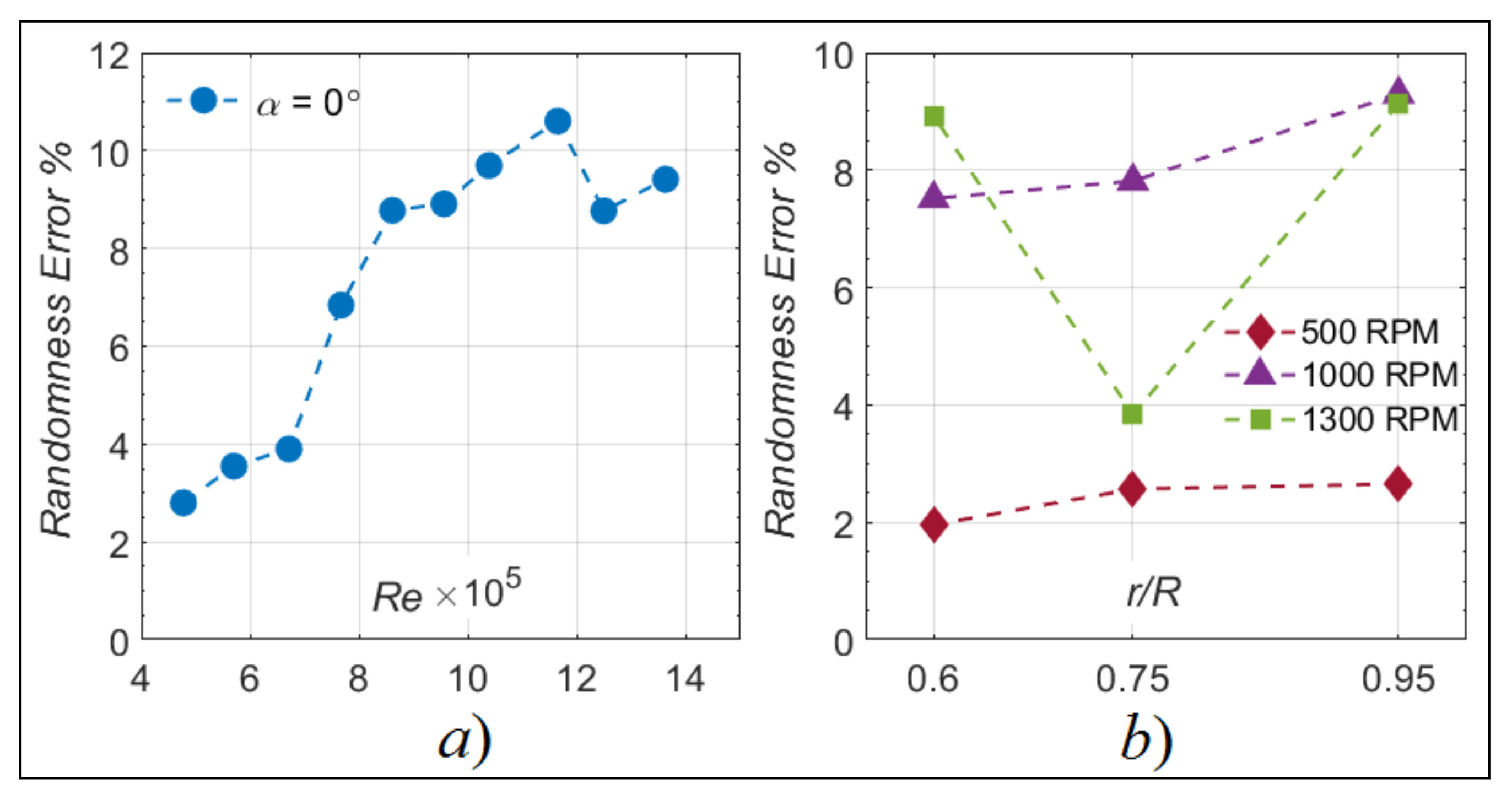
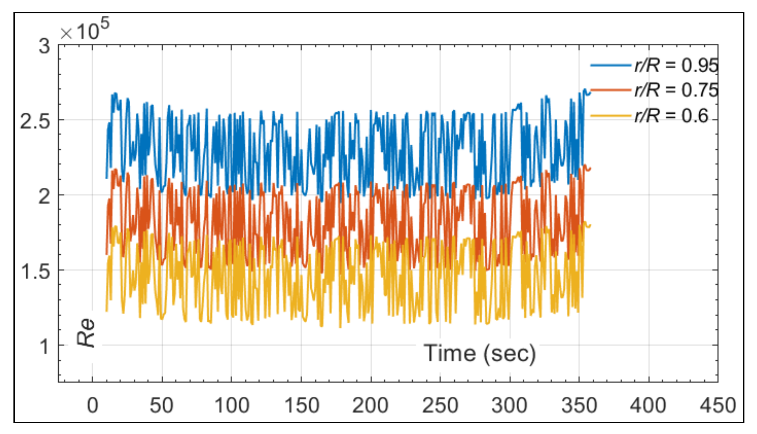
Previous studies that correlated Fr_x with Re (using Equation (1)) were all made using non-rotating geometries, and the Re was mostly constant during the test. Contrary to a fixed-wing, the Re for rotating blades varies during the test. As an example, Figure 18 shows the variation of the calculated Re (Equation (5)) at the three r/R of rotor test #2 versus time. Because of the freestream velocity and blade rotation, the Re depends on Ω, V_∝ and r/R. This triple dependency creates relatively large variations of the Re, as shown in Figure 18, where the Re increases when the blade is on the advancing side and decreases on the retreating side of the blade. 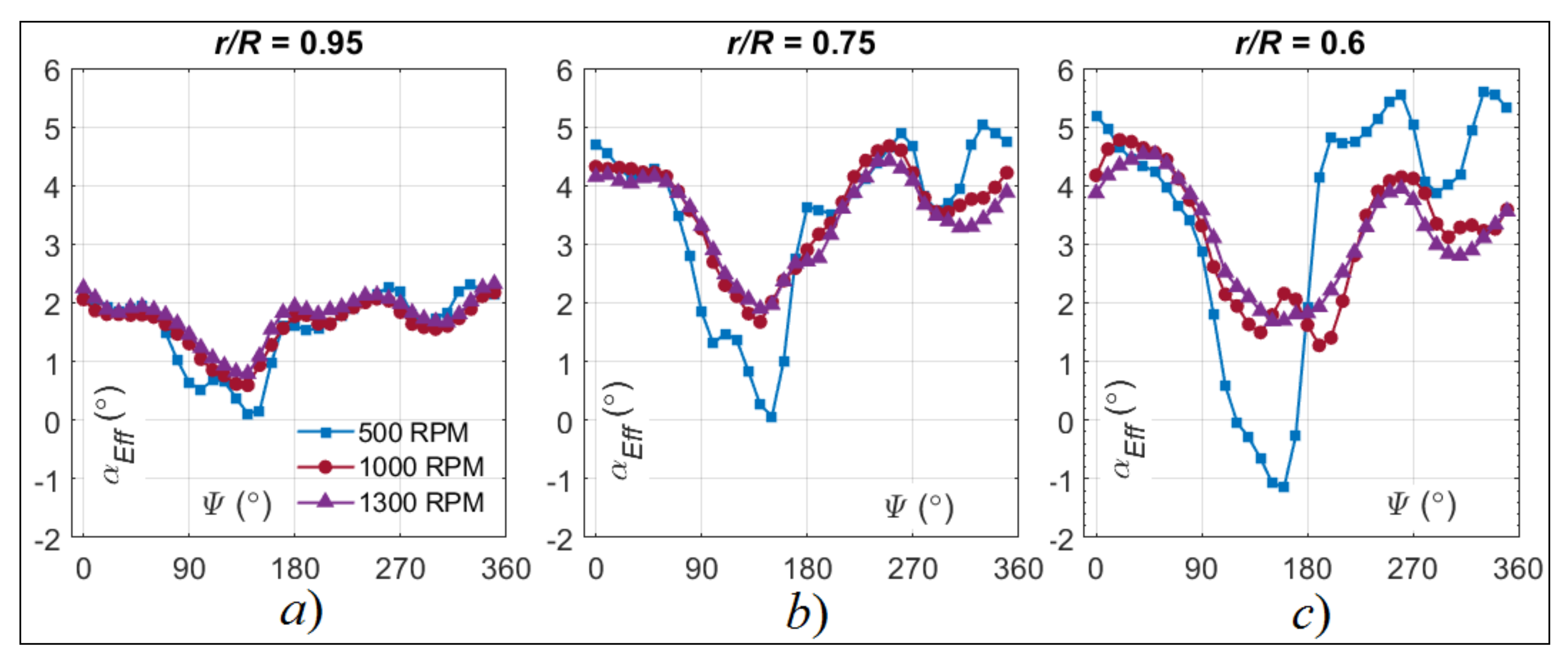This goes in parallel with variations of the α_Eff, as shown in Figure 17 for the same reasons.

In this study, the proposed correlations were built based on the averaged values of Fr, Re, and α_Eff. (Re_Avg) is defined as the average value of Re of each test and radial position and is calculated the mean of the varying Re, as shown in Figure 18. Similarly, the average values of α_Eff from Figure 17 are also used. The range of Re_Avg is between 9.5 × 10⁴ ≤ Re_Avg ≤ 3.71 × 10⁵ corresponding to the lowest Re_Avg at r/R = 0.6 for Ω = 500 RPM and the highest at r/R = 0.95 for Ω = 1500 RPM.

The first correlation attempt was for the tests at θ = 0° given that the α_Eff = 0° throughout the blade. This way, the correlation is expected to satisfy the form of Equation (1). In this study, the Fr_x was correlated with Re_Avg at each S/c. Curve fitting was carried out using MATLAB, and the correlation constants A and m are presented in

Table 10. Constants for curve fitting Fr_x = A × (Re_Avg)^m× Pr^1/3 of rotor experimental data at θ = 0°.

S/c	0	0.15	0.30	0.44
A	0.020	0.022	0.011	0.010
m	0.369	0.329	0.399	0.399
Error %	3.54%	2.14%	3.71%	7.69%

, together with the average error found between the experimental data and the correlation prediction. The Pr used was the one at T_∞ = 248.15 K and is equal to Pr = 0.70.

If the parameters are analyzed, it is found that for θ = 0°, the Fr_x correlates with Re_Avg by 0.369 ≤ m ≤ 0.399 at all S/c. This contradicts the results of [8], who obtained m = 0 at the stagnation point and laminar region downstream for a fixed-wing airfoil with α = 0°. Furthermore, the range of m for θ = 6° is 0.220 ≤ m ≤ 0.373, which is also not expected near the leading edge of the airfoil. These values for m could only be explained by the relatively high TI found in the rotor tests. Turbulent heat transfer augmentation is a direct result of the TI that, according to [14], affects the stagnation, laminar, and turbulent regions of flows on airfoils.

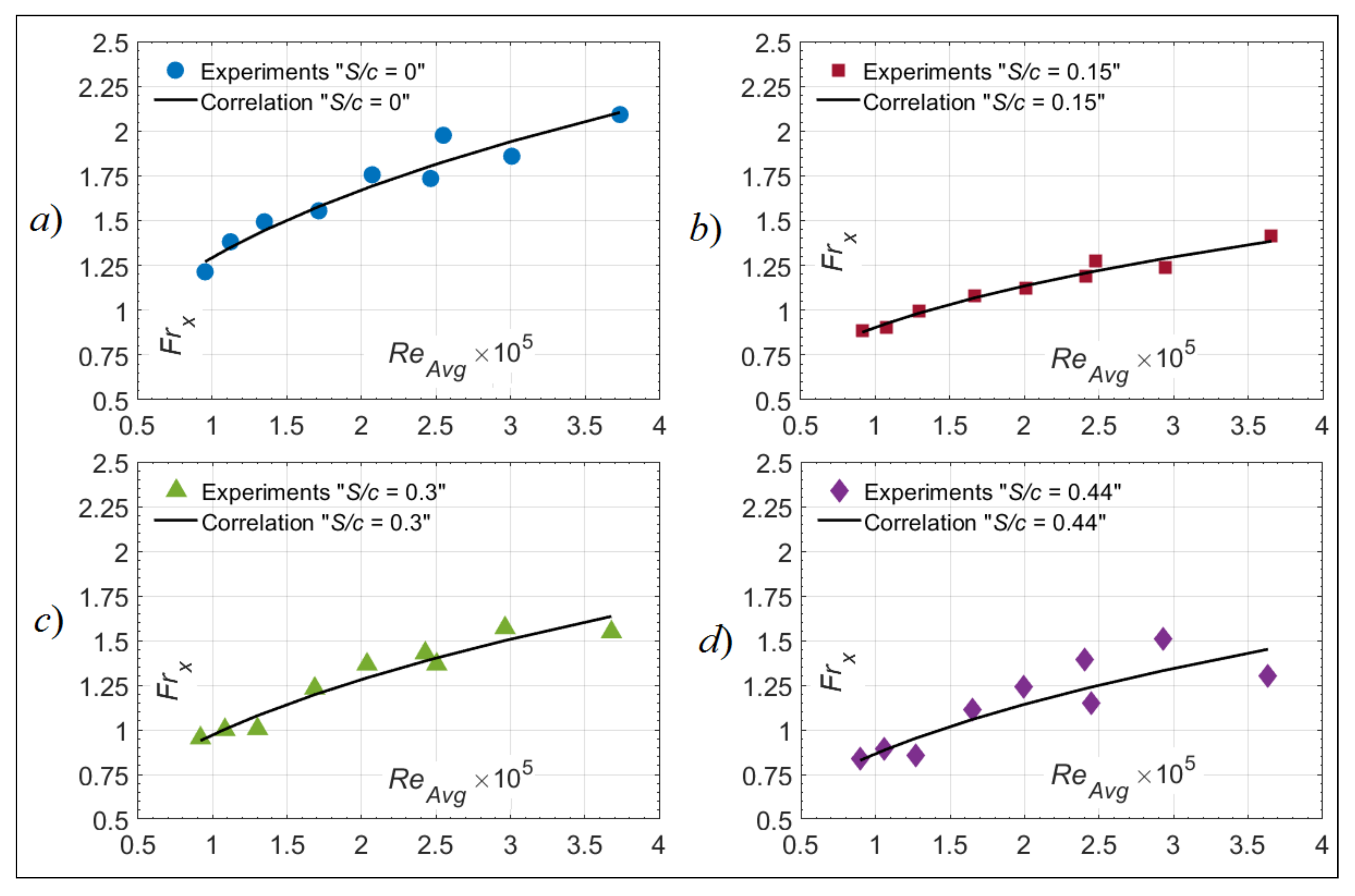
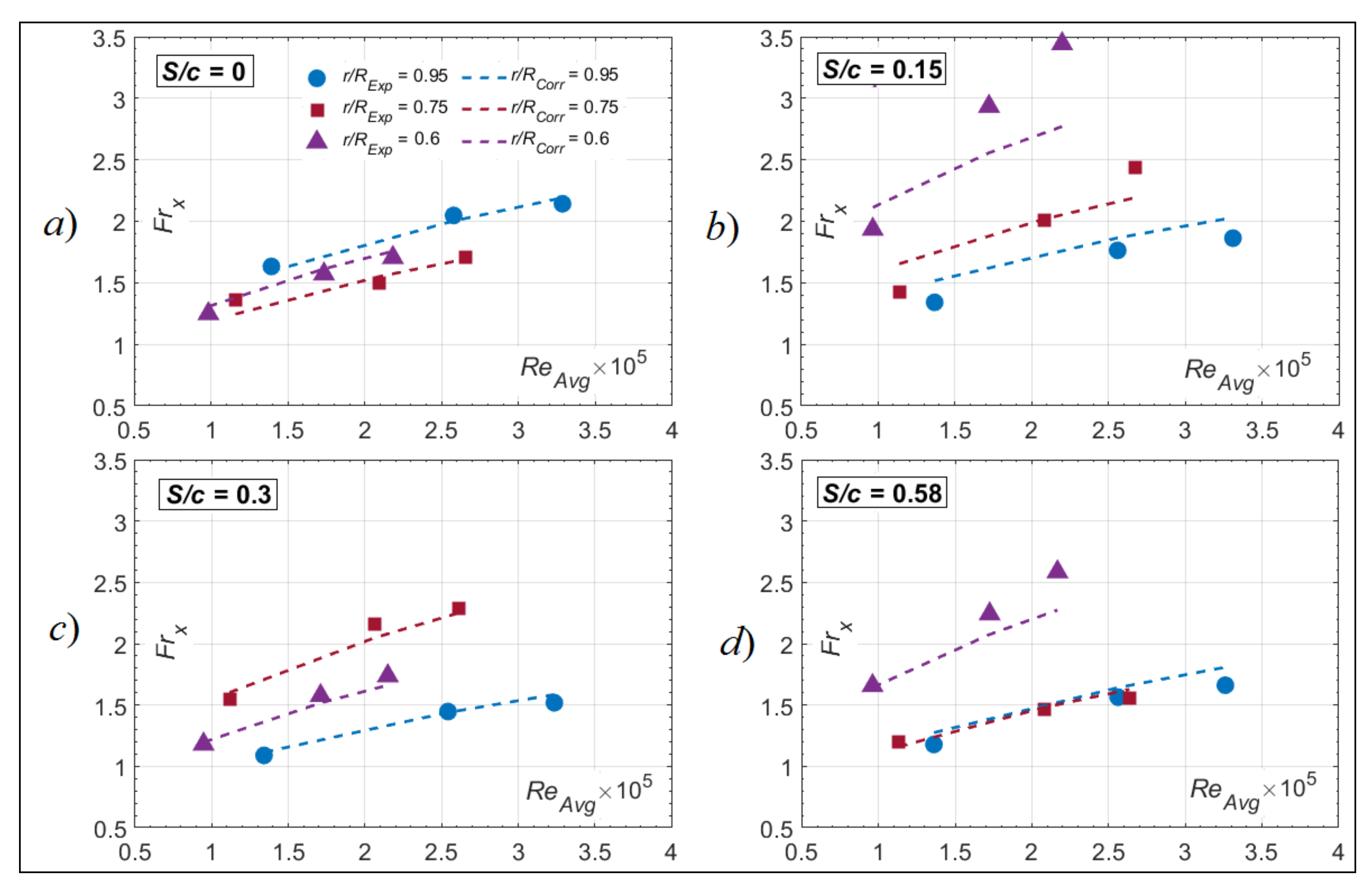
Figure 19 shows a graphical representation of the correlations in Table 10, compared to the measured values of Fr_x for each S/c at θ = 0°. The correlations fit very well the data, with an average error between 2.14% and 7.69%. This was also the case in [8], where the fitting of the fixed-wing data at α = 0° and different S/c was successful, and with a similar average error similar to the one found for the rotor at θ = 0°. Recalling that the correlations are fit based on Equation (1) and that the α_Eff = 0° for the non-lifting rotor, then Figure 19 proves that the possibility of correlating rotor data only with Re_Avg is successful.

Because the aim of this paper is to propose a correlation for the Fr_x in terms of the Re and α_Eff, the data for the rotor tests at θ = 6° are now fitted in the form of Equation (23), which is a generalized form of Equation (2) for the BEMT–RHT and UVLM–RHT. The A and m parameters used were the ones from the tests at θ = 0°, and the values of α_Eff (converted to radians) were the ones determined through the UVLM calculations from Section 3.4. For the tests at θ = 0°, the α_Eff is 0° throughout the blade and Equation (23) reduces to the same correlations previously presented in Table 10. This way, Equation (23) could be used to calculate the Fr_x at any blade section, even when the α_Eff varies with θ.

$$F{r}_x=A\times \left(1+C_1\times {\alpha }_{Eff}+C_2\times {\alpha }_{Eff}^2\right){\mathrm{Re}}^m{\mathrm{Pr}}^{1/3}$$

(23)

The curve fitting of Equation (23) was applied for each S/c of the tests at θ = 6°, and the results for C₁ and C₂ are presented in

Table 11. Constants for curve fitting Fr_x = A × (1 + C₁ × α_Eff + C₂ × α²_Eff) × (Re_Avg)^m× Pr^1/3 of rotor experimental data at θ = 6°.

S/c	A	m	C1	C2	Error %
0	0.020	0.369	12.08	−215.50	3.31%
0.15	0.022	0.329	6.31	149.43	14.97%
0.30	0.011	0.399	−22.22	514.38	3.00%
0.58	0.010	0.399	−15.17	−167.31	7.11%

along with the average error between the experimental data and correlation predictions. Figure 20 also shows a graphical representation of the comparison between the predictions of Equation (23) and the experimental data at θ = 6°. At S/c = 0, S/c = 0.30, and S/c = 0.58, the correlation fits the data very well and within 3% to 7% error. For S/c = 0.15, the error is higher, i.e., just under 15%. By examining Figure 20, the elevated error originates mostly from a single test at r/R = 0.6. Given the experimental error involved, however, it is believed an acceptable estimate of the Fr_x can be obtained with the novel correlation of Equation (23).

5. Conclusions

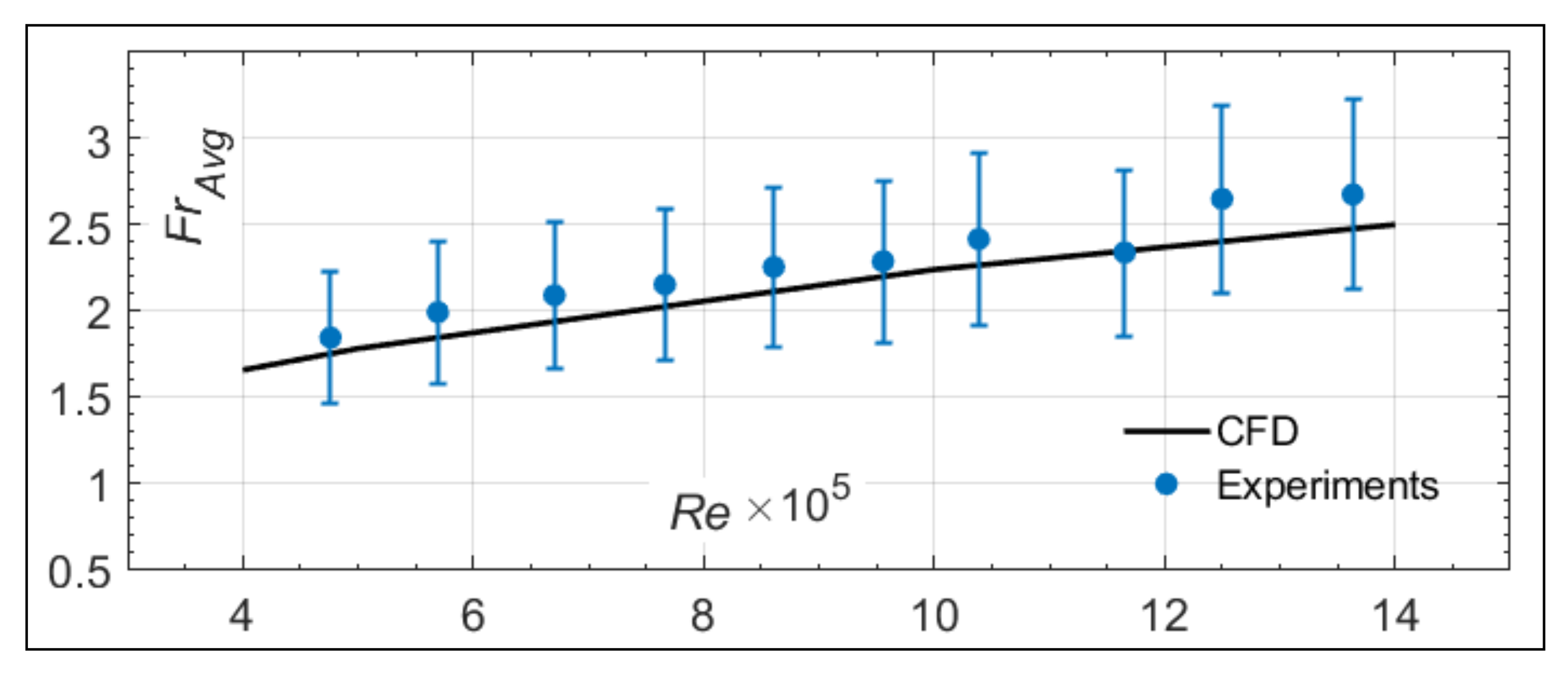
This paper presented heat transfer measurements made on the surfaces of a fixed-wing and a small two-blade rotor. The goal of this study was to propose correlations for the experimentally measured rotor Fr_x values based on Re and α_Eff. The fixed-wing tests were used to verify the heat transfer measurements in the IWT and had a total experimental between 16% and 21%. Results indicate that the fixed-wing Fr_x at the stagnation point was in the range of experimental data from the literature, and within 8% of fully turbulent CFD simulations. The Fr_Avg also agrees with CFD predictions, with an average discrepancy of 1.4%.

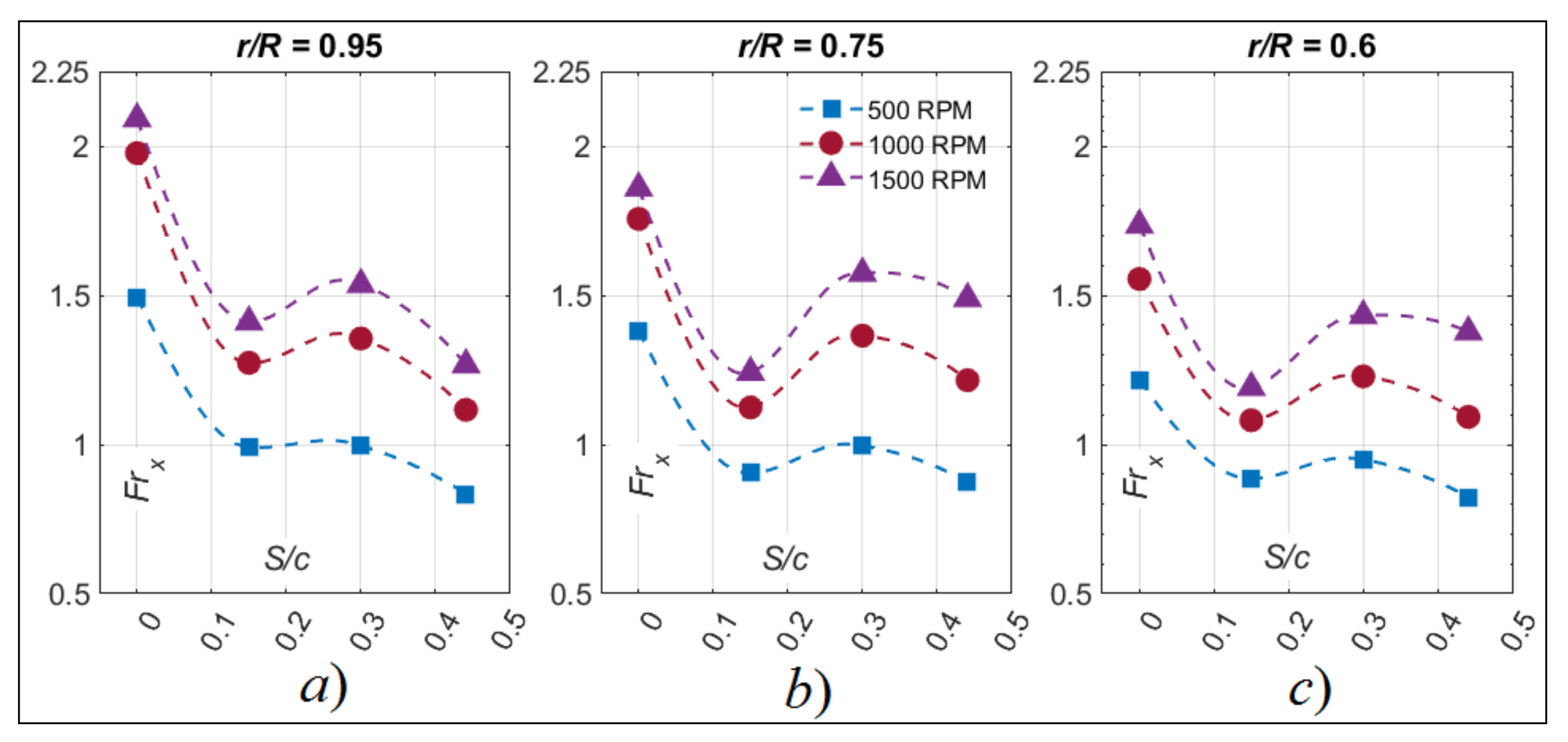
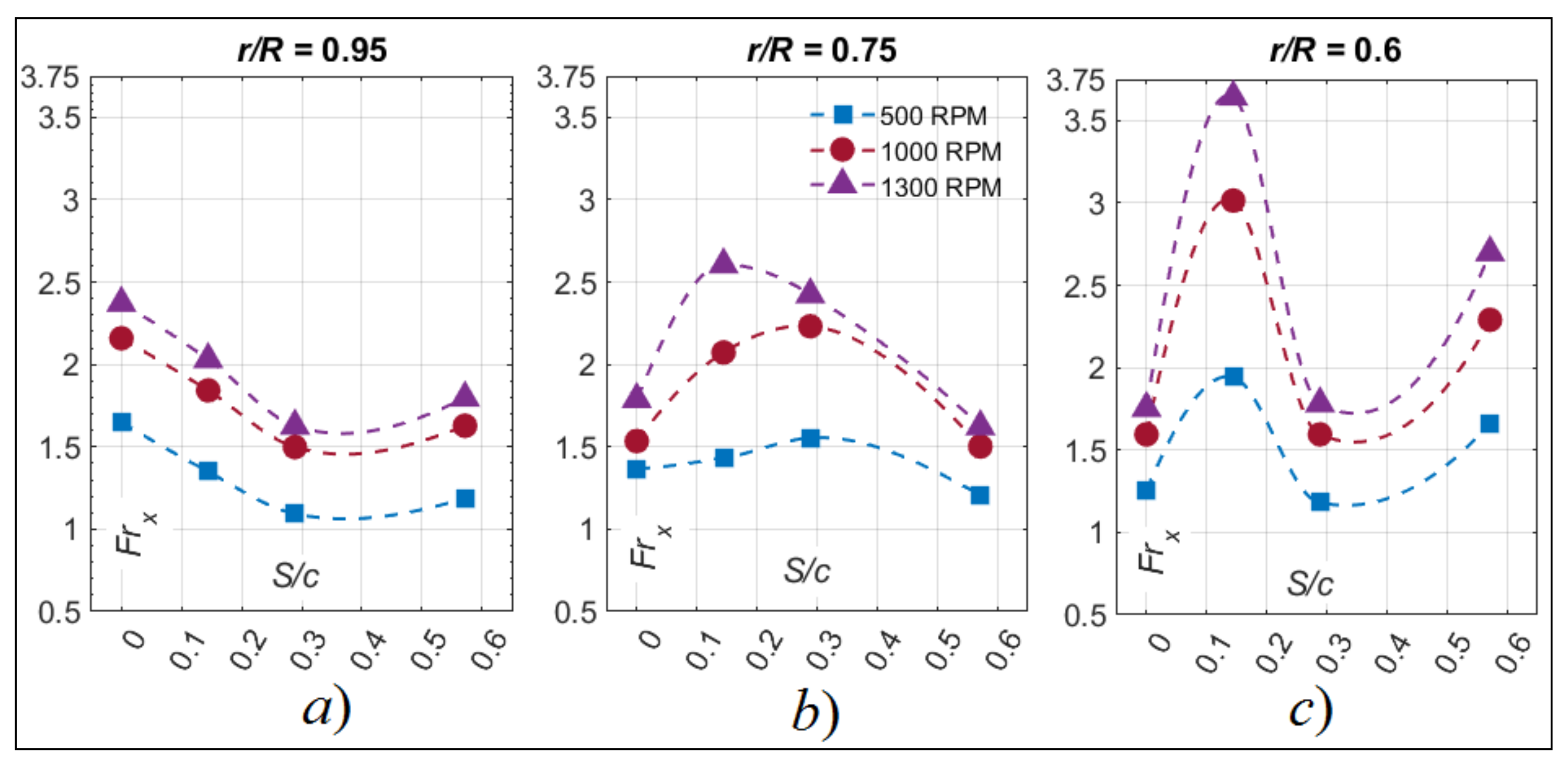
For the rotor tests, the total experimental error was estimated at 25%. The Ω directly increased the Fr_x values for all rotor tests due to an increase of Re. The rotor tests at θ = 0° showed that Fr_x behavior was rather insensitive to changes in r/R whereas the behavior changed significantly between r/R for the tests at θ = 6°. As the UVLM–RHT simulations proved, this was due to the varying α_Eff across the blade for the tests with the positive pitch angle, whereas for the non-lifting rotor, the α_Eff is 0° from root to tip.

The Fr_x data from the tests at θ = 0° were successfully correlated with Re at each S/c and with an error between 2.14% to 7.69%. When a term for the α_Eff was incorporated, a novel correlation for the Fr_x (at each S/c) in the form of Equation (23) that satisfies the data at θ = 0° and θ = 6° could then be formed and with a maximum error 14%. The results of this paper, therefore, show that the Fr_x across the rotor blade could be successfully correlated with Re and α_Eff; thus, justifying the methodology implemented in the previously developed BEMT–RHT and UVLM–RHT.

On a side note, the Fr_x correlations with Re^m_Avg showed values of m that are consistently larger than 0.329. Given the locations of measurements and the range of Re involved, it was expected that some of the proposed correlations show values of m = 0, which is expected for laminar flow on flat plates or fixed-wing airfoils. The relatively high TI values are suspected to be the reason for this, which could eventually cause heat transfer augmentation and therefore explain the Fr_x variation with Re. In this study, no corrections for TI were implemented, and further investigation is recommended.

Future work in this research project includes further testing of the present rotor setup but under icing conditions. Several ice-accreting/de-icing tests will be run and compared to the presently ice-free heat transfer measurements. The gathered data will be studied and included in the BEMT–RHT and UVLM–RHT to account for heat transfer calculation under icing conditions.

References

1. Esmeryan, K.D. From Extremely Water-Repellent Coatings to Passive Icing Protection—Principles, Limitations and Innovative Application Aspects. J. Coat. 2020, 10, 66. [Google Scholar] [CrossRef] [Green Version]
2. Cao, Y.; Tan, W.; Wu, Z. Aircraft icing: An ongoing threat to aviation safety. Aerosp. Sci. Technol. 2018, 75, 353–385. [Google Scholar] [CrossRef]
3. Tarquini, S.; Antonini, C.; Amirfazli, A.; Marengo, M.; Palacios, J. Investigation of ice shedding properties of superhydrophobic coatings on helicopter blades. Cold Reg. Sci. Technol. 2014, 100, 50–58. [Google Scholar] [CrossRef]
4. Lavoie, P.; Pena, D.; Hoarau, Y.; Laurendeau, E. Comparison of thermodynamic models for ice accretion on airfoils. Int. J. Numer. Methods Heat Fluid Flow 2018, 28, 1004–1030. [Google Scholar] [CrossRef]
5. Bergman, T.L.; Incropera, F.P.; DeWitt, D.P.; Lavine, A.S. Fundamentals of Heat and Mass Transfer, 7th ed.; John Wiley & Sons: New York, NY, USA, 2007. [Google Scholar]
6. Kays, W.M.; Crawford, M. Convective Heat and Mass Transfer, 3rd ed.; McGraw-Hill: New York, NY, USA, 1993. [Google Scholar]
7. Lienhard, J. Heat transfer in flat-plate boundary layers: A correlation for laminar, transitional and turbulent flow. Heat Trans. 2020, 142, 061805. [Google Scholar] [CrossRef] [Green Version]
8. Poinsatte, P.E.; Newton, J.E.; De Witt, K.J.; Van Fossen, G.J. Heat transfer measurements from a smooth NACA 0012 airfoil. J. Aircr. 1991, 28, 892–898. [Google Scholar] [CrossRef]
9. Wang, X.; Bibeau, E.; Naterer, G. Experimental correlation of forced convection heat transfer from a NACA airfoil. Exp. Therm. Fluid Sci. 2007, 31, 1073–1082. [Google Scholar] [CrossRef]
10. Wang, X.; Naterer, G.; Bibeau, E. Convective Heat Transfer from a NACA Airfoil at Varying Angles of Attack. J. Thermophys. Heat Transf. 2008, 22, 457–463. [Google Scholar] [CrossRef]
11. Wang, X.; Naterer, G.F.; Bibeau, E. Convective Droplet Impact and Heat Transfer from a NACA Airfoil. J. Thermophys. Heat Transf. 2007, 21, 536–542. [Google Scholar] [CrossRef]
12. Wang, X.; Naterer, G.; Bibeau, E. Multiphase Nusselt Correlation for the Impinging Droplet Heat Flux from a NACA Airfoil. J. Thermophys. Heat Transf. 2008, 22, 219–226. [Google Scholar] [CrossRef]
13. Li, G.; Gutmark, E.J.; Ruggeri, R.T.; Mabe, J.H. Heat Transfer and Pressure Measurements on a Thick Airfoil. J. Aircr. 2009, 46, 2130–2138. [Google Scholar] [CrossRef]
14. Van Fossen, G.J.; Simoneau, R.J.; Ching, C.Y. Influence of Turbulence Parameters, Reynolds Number, and Body Shape on Stagnation-Region Heat Transfer. J. Heat Transf. 1995, 117, 597–603. [Google Scholar] [CrossRef] [Green Version]
15. Narducci, R.; Kreeger, R.E. Application of a High-Fidelity Icing Analysis Method to a Model-Scale Rotor in Forward Flight; NASA: Virginia Beach, VA, USA, 2012.
16. Palacios, J.L.; Han, Y.; Brouwers, E.W.; Smith, E.C. Icing Environment Rotor Test Stand Liquid Water Content Measurement Procedures and Ice Shape Correlation. J. Am. Helicopter Soc. 2012, 57, 29–40. [Google Scholar] [CrossRef]
17. Tsao, J.C.; Kreeger, R.E. Further Evaluation of Scaling Methods for Rotorcraft Icing; NASA Glenn Research Center: Cleveland, OH, USA, 2012.
18. Wang, Z.; Zhu, C.; Zhao, N. Experimental Study on the Effect of Different Parameters on Rotor Blade Icing in a Cold Chamber. Appl. Sci. 2020, 10, 5884. [Google Scholar] [CrossRef]
19. Wright, J.; Aubert, R. Icing wind tunnel test of a full scale heated tail rotor model. In Proceedings of the AHS 70th Annual Forum, Montreal, QC, Canada, 20–22 May 2014; pp. 20–22. [Google Scholar]
20. Aubert, R. Additional Considerations for Analytical Modeling of Rotor Blade Ice. In Proceedings of the SAE 2015 International Conference on Icing of Aircraft, Engines, and Structures, Prague, Czech Republic, 22–25 June 2015. [Google Scholar]
21. Samad, A.; Tagawa, G.B.S.; Morency, F.; Volat, C. Predicting Rotor Heat Transfer Using the Viscous Blade Element Momentum Theory and Unsteady Vortex Lattice Method. Aerospace 2020, 7, 90. [Google Scholar] [CrossRef]
22. SAE. Calibration and Acceptance of Icing Wind Tunnels; Aerospace Standard ARP5905. 2003, AC-9C Aircraft Icing Technology Committee; SAE International: Warrendale, PA, USA, 2003. [Google Scholar]
23. SAE. Droplet Sizing Instrumentation Used in Icing Facilities; Aerospace Standard AIR4906. 1995, AC-9C Aircraft Icing Technology Committee; SAE International: Warrendale, PA, USA, 1995. [Google Scholar]
24. Fortin, G.; Perron, J. Spinning Rotor Blade Tests in Icing Wind Tunnel. American Institute of Aeronautics and Astronautics. In Proceedings of the 1st AIAA Atmospheric and Space Environments Conference, San Antonio, TX, USA, 22–25 June 2009; p. 4260. [Google Scholar]
25. IEC Corporation—Slip Ring Assemblies. Flange mount slip ring. Austin, Texas, USA. Available online: https://ieccorporation.com/flange-mount/ (accessed on 23 December 2020).
26. Eckert, E. Engineering relations for heat transfer and friction in high-velocity laminar and turbulent boundary-layer flow over surfaces with constant pressure and temperature. Trans. ASME 1956, 78, 1273–1283. [Google Scholar]
27. Omega Engineering. Polyimide Insulated Flexible Heaters; Self-Adhesive Polyimide Flexible Heaters 302°F Max. 2021. Available online: https://www.omega.ca/en/industrial-heaters/surface-heaters/flexible-heaters/p/KHRA-KHLVA-KHA-SERIES. (accessed on 11 February 2021).
28. Yeh, F.C.; Hippensteele, S.A.; Van Fossen, G.J.; Poinsatte, P.E.; Ameri, A. High Reynolds number and turbulence effects on turbine heat transfer. J. Propuls. Power 1994, 10, 868–875. [Google Scholar] [CrossRef]
29. Moffat, R.J. Describing the uncertainties in experimental results. Exp. Therm. Fluid Sci. 1988, 1, 3–17. [Google Scholar] [CrossRef] [Green Version]
30. Ames, F.E.; Kulacki, F.A. Turbulence Effects on Convective Heat Transfer; Springer International Publishing: New York, NY, USA, 2017; pp. 1–33. [Google Scholar]
Figure 1. Icing wind tunnel (IWT) schematic [24].
Aerospace 08 00053 g001
Figure 2. NACA 0012 airfoil in the IWT test section.
Aerospace 08 00053 g002
Figure 3. NACA 0012 convection tests with outer heating elements and RTDs locations.
Aerospace 08 00053 g003
Figure 4. NACA 0012 conduction tests with inner RTDs locations.
Aerospace 08 00053 g004
Figure 5. The aluminum tape covering the heating elements and the blade with three RTDs is shown.
Aerospace 08 00053 g005
Figure 6. Sketch of the experimented blade with radial positions of interest.
Aerospace 08 00053 g006
Figure 7. Sketch of experimented blade cross section with chordwise positions of interest.
Aerospace 08 00053 g007
Figure 8. Heat conduction approximation of airfoil surface to (a) cylinder (b) flat plate.
Aerospace 08 00053 g008
Figure 9. Air and RTDs temperature variation versus time for fixed-wing test #3.
Aerospace 08 00053 g009
Figure 10. Frx variation for all RTDs versus time for fixed wing test #3.
Aerospace 08 00053 g010
Figure 11. Computed randomness error for (a) fixed-wing and (b) rotor tests.
Aerospace 08 00053 g011
Figure 12. Calculated turbulence intensity for (a) rotor tests at S/c = 0 for different θ, Ω, and r/R and (b) fixed-wing tests for 4.76 × 10⁵Re ≤ 1.36 × 10⁶.
Aerospace 08 00053 g012
Figure 13. Comparison of stagnation point (S/c = 0) measurements at α = 0° versus CFD [21] and NACA 0012 experimental data [8].
Aerospace 08 00053 g013
Figure 14. Results of experimentally measured FrAvg over fixed-wing compared to fully turbulent CFD simulations [21] for a range of 4.76 × 10⁵Re ≤ 1.36 × 10⁶.
Aerospace 08 00053 g014
Figure 15. Chordwise variation of Frx at θ = 0°, for three rotor speeds (Ω = 500 RPM, 1000 RPM, and 1500 RPM) at three different radial locations (a) r/R = 0.95, (b) 0.75, and (c) 0.6.
Aerospace 08 00053 g015
Figure 16. Chordwise variation of Frx at θ = 6°, for three rotor Speeds (Ω = 500 RPM, 1000 RPM, and 1300 RPM) at three different radial locations (a) r/R = 0.95, (b) 0.75, and (c) 0.6.
Aerospace 08 00053 g016
Figure 17. UVLM–RHT Results of the αEff variation with Ψ for the rotor tests for = 500 RPM, 1000 RPM, and 1300 RPM at (a) r/R = 0.95, (b) r/R = 0.75, and (c) r/R = 0.6.
Aerospace 08 00053 g017
Figure 18. Example of the Re variation versus time at the three blade sections r/R = 0.6, 0.75, and 0.95 for test #2 (Ω = 1000 RPM, θ = 0°, and V = 5 m/s).
Aerospace 08 00053 g018
Figure 19. Correlation attempts with Frx = A×(ReAvg)m×Pr1/3 for rotor tests at θ = 0° and at (a) S/c = 0, (b) S/c = 0.15, (c) S/c = 0.3, and (d) S/c = 0.44.
Aerospace 08 00053 g019
Figure 20. Correlation attempts with Frx = A × (1 + C1 × αEff + C2 × α2Eff) × (ReAvg)m× Pr1/3 for rotor tests at θ = 6° and (a) S/c = 0, (b) S/c = 0.15, (c) S/c = 0.3, and (d) S/c = 0.58.
Aerospace 08 00053 g020