Article

Analysis of Aircraft Routing Strategies for North Atlantic Flights by Using AirTraf 2.0

1
Deutsches Zentrum für Luft- und Raumfahrt, Institut für Physik der Atmosphäre, 82234 Oberpfaffenhofen, Germany
2
Aerospace Engineering, Section Aircraft Noise and Climate Effects, Delft University of Technology, 2629 HS Delft, The Netherlands
*
Author to whom correspondence should be addressed.
Aerospace 2021, 8(2), 33; https://doi.org/10.3390/aerospace8020033
Submission received: 30 October 2020 / Revised: 19 January 2021 / Accepted: 23 January 2021 / Published: 28 January 2021

Abstract

:
Climate-optimized routing is an operational measure to effectively reduce the climate impact of aviation with a slight increase in aircraft operating costs. This study examined variations in the flight characteristics among five aircraft routing strategies and discusses several characteristics of those routing strategies concerning typical weather conditions over the North Atlantic. The daily variability in the North Atlantic weather patterns was analyzed by using the European Center Hamburg general circulation model (ECHAM) and the Modular Earth Submodel System (MESSy) Atmospheric Chemistry (EMAC) model in the specified dynamics mode from December 2008 to August 2018. All days of the ten complete winters and summers in the simulations were classified into five weather types for winter and into three types for summer. The obtained frequency for each of the weather types was in good agreement with the literature data; and then representative days for each weather type were selected. Moreover, a total of 103 North Atlantic flights of an Airbus A330 aircraft were simulated with five aircraft routing strategies for each representative day by using the EMAC model with the air traffic simulation submodel AirTraf. For every weather type, climate-optimized routing shows the lowest climate impact, at which a trade-off exists between the operating costs and the climate impact. Cost-optimized routing lies between the time- and fuel-optimized routings and achieves the lowest operating costs by taking the best compromise between flight time and fuel use. The aircraft routing for contrail avoidance shows the second lowest climate impact; however, this routing causes extra operating costs. Our methodology could be extended to statistical analysis based on long-term simulations to clarify the relationship between the aircraft routing characteristics and weather conditions.

Graphical Abstract

1. Introduction

The climate impact due to aviation emissions [1,2,3,4] is expected to increase further in response to strong growth in the demand for the aviation sector from a long-term perspective [5]. Climate-optimized routing has been proposed as an important measure for reducing the climate impact of aviation [6,7,8]. This routing significantly reduces the climate impact by optimizing flight routes to detour regions where released emissions and formed contrails have a large climate impact. An advantage of the climate-optimized routing is that the routing is immediately applicable to the current fleet of aircraft without large costs of renewing the fleet. Technological measures (e.g., efficient engines, blended wing–body configurations, laminar flow controls, and sustainable fuels; [9,10]) also have an important role in reducing the climate impact of aviation; however, the implementation of those measures is a long-term effort. Both climate-optimized routing and the technological measures are required to effectively reduce the climate impact of aviation. A number of studies have been carried out regarding climate-optimized routing [7,11]. Lührs et al. [12] performed flight trajectory optimization for nine sample trans-Atlantic routes for a specific weather pattern in winter by the Trajectory Optimization Module (TOM; [12]). They showed that the climate-optimum trajectory (3D-optimized trajectory in the lateral and vertical directions) decreased the climate impact by about 45% over that of the economical route, whereas it increased the cash operating cost (COC; [13]) by 2%. Ng et al. [14] examined climate-optimized routing for 960 transatlantic flights (482 eastbound and 478 westbound flights) for a specific summer day. The absolute global temperature change potential (AGTP for the time horizon of 50 years) due to CO2 emissions and contrails was considered. They showed that the routing decreased the total AGTP by 38% with an additional flight time of 3.1% and with an extra fuel use of 3.1% for the eastbound flights. Similarly, the routing decreased the total AGTP by 20% with an additional flight time of 3.0% and with the extra fuel use of 3.7% for the westbound flights. As aircraft operating costs generally depend on time and fuel, those results indicate a cost increase. Many studies reported the benefit of climate-optimized routing, but the routing increases aircraft operating costs; that is, a trade-off exists between economic costs and the climate impact. The trade-off, in fact, seems to be severe, because a cost reduction is a primary concern for airlines; however, if additional costs for the climate impact of aviation, such as environmental taxes, are included in the current operating costs, a cost increase due to climate-optimized routing is possibly compensated [7]. This inclusion can change the current routing strategy of minimum costs and incentivize airlines to introduce climate-optimized flight planning.
There are two other important routing strategies for aircraft operations. One is a cost-optimized routing. Today’s flight planning is implemented on the basis of minimum economic costs, which are related to two factors: flight time and fuel use. Generally, a trade-off exists between the flight time and fuel use. Celis et al. [15] compared performances for the time optimum and the fuel optimum trajectories under the International Standard Atmospheric (ISA) conditions. A typical single-aisle aircraft configuration (150 passengers) with twin turbofan engines was assumed; the aircraft speed and the flight altitude in eight flight segments were optimized for a given flight trajectory (a quasi-full flight profile optimization). They showed that the fuel optimum trajectory experienced a decrease in fuel use of 31.7 percentage points with an increase in flight time of 14.0 percentage points over those of the time optimum trajectory. Rosenow and Fricke [16] carried out a flight trajectory optimization on the flight time and on the fuel use for a flight from Frankfurt (Main) to Dubai for a Boeing B777 freighter on 2 February, 2016, at 12:00 GMT. The results showed that the fuel optimum trajectory decreased the fuel use by 8.0% with an increased flight time of 3.7%. As it is difficult to decrease both factors simultaneously, one has to find the best compromise between the two factors to minimize the overall operating costs.
The other important routing strategy is contrail avoidance, which is expected to reduce the climate impact of aviation [17,18,19,20,21]. Soler et al. [22] examined an optimal flight trajectory for mitigating the climate impact of aviation by considering persistent contrail formation areas (PCFAs). A flight from San Francisco (SFO) to New York (JFK) for a Boeing B757-200 aircraft was considered; the wind data on 17 March, 2014 were employed; and the temperature and relative humidity on 30 June, 2012 were used to construct PCFAs. They showed that the contrail mitigation strategy cost approximately USD 360 for extra fuel use and USD 1010 for an additional flight time compared to those of the minimum cost strategy (scenarios with time horizons of 20 and 100 years for the global warming potential of contrails). Rosenow et al. [23] optimized a one-day European air traffic on 25 July 2016. The total number of 13,584 flights over Europe (containing 16 aircraft types) was employed; their three-dimensional flight profiles were optimized for airline costs (termed as the cost performance indicators, CPIs) and environmental impacts (termed as the ecological performance indicators, EPIs). They showed that an additional contrail avoidance intent decreased contrail costs by 31.5% (contrail formations were converted into a monetary value) and EPIs by 5.2%, whereas the intent increased the fuel use by 0.05% and CPIs by 0.5% over those of the minimum cost strategy. Many previous studies reported that the routing for contrail avoidance reduces the climate impact; however, this routing increases aircraft operating costs.
Now, the question arises, “Do such characteristics of those routing strategies always exist, when different weather conditions are considered?” Clearly the quantitative values of flight characteristics (such as flight time, fuel use, operating costs, and climate impact) vary, depending on the atmospheric conditions during a flight, whereas different target days (atmospheric conditions) are chosen for every study, respectively. To our knowledge, there are few systematic studies that investigate the relationship between aircraft routing characteristics and weather systems. The ultimate aim of our study is twofold: to investigate whether such characteristics of the aircraft routing strategies are common under any atmospheric conditions and to systematically investigate the relationship between the aircraft routing characteristics and weather conditions. These investigations could identify the weather condition that achieves a large reduction in the climate impact when the climate-optimized routing strategy is employed.
As the first step for these aims, this study examined several common characteristics of the aircraft routing strategies under typical weather conditions over the North Atlantic region. We focused on this region because the air space over the North Atlantic is one of the busiest and the most important oceanic air spaces in the world. Moreover, the benefits of climate-optimized routing are high for this region [6,7,8,11]. The daily variability in the North Atlantic weather patterns is analyzed by using the European Center Hamburg general circulation model (ECHAM) and the Modular Earth Submodel System (MESSy) Atmospheric Chemistry (EMAC) model [24,25], and representative days that show typical weather types of the region are determined. Then, a total of 103 North Atlantic flights were simulated by using the EMAC model with the air traffic simulation submodel AirTraf [26,27,28]. AirTraf can simulate air traffic for various aircraft routing strategies under comprehensive atmospheric conditions calculated by EMAC. Here, the air traffic simulations are performed with respect to five aircraft routing strategies, which include the time optimal, fuel optimal, cost optimal, contrail avoidance and climate optimal strategies, for the representative days of each weather type. To reveal the characteristics of those aircraft routing strategies, which are common to all the representative days, variations in typical flight characteristics obtained from those air traffic simulations were analyzed.
This paper is organized as follows: Section 2 presents a brief description of the numerical models and methods used for weather pattern analysis and air traffic simulations (the flight trajectory optimization method is described in Appendix A). Section 3 validates the weather pattern analysis and presents the characteristics of the North Atlantic weather patterns. Section 4 presents the results regarding the characteristics of the aircraft routing strategies concerning the weather patterns. Section 5 discusses the limitations of the simulation results and the further development of our model towards multi-objective flight trajectory optimizations. Finally, Section 6 concludes this study.

2. Methods

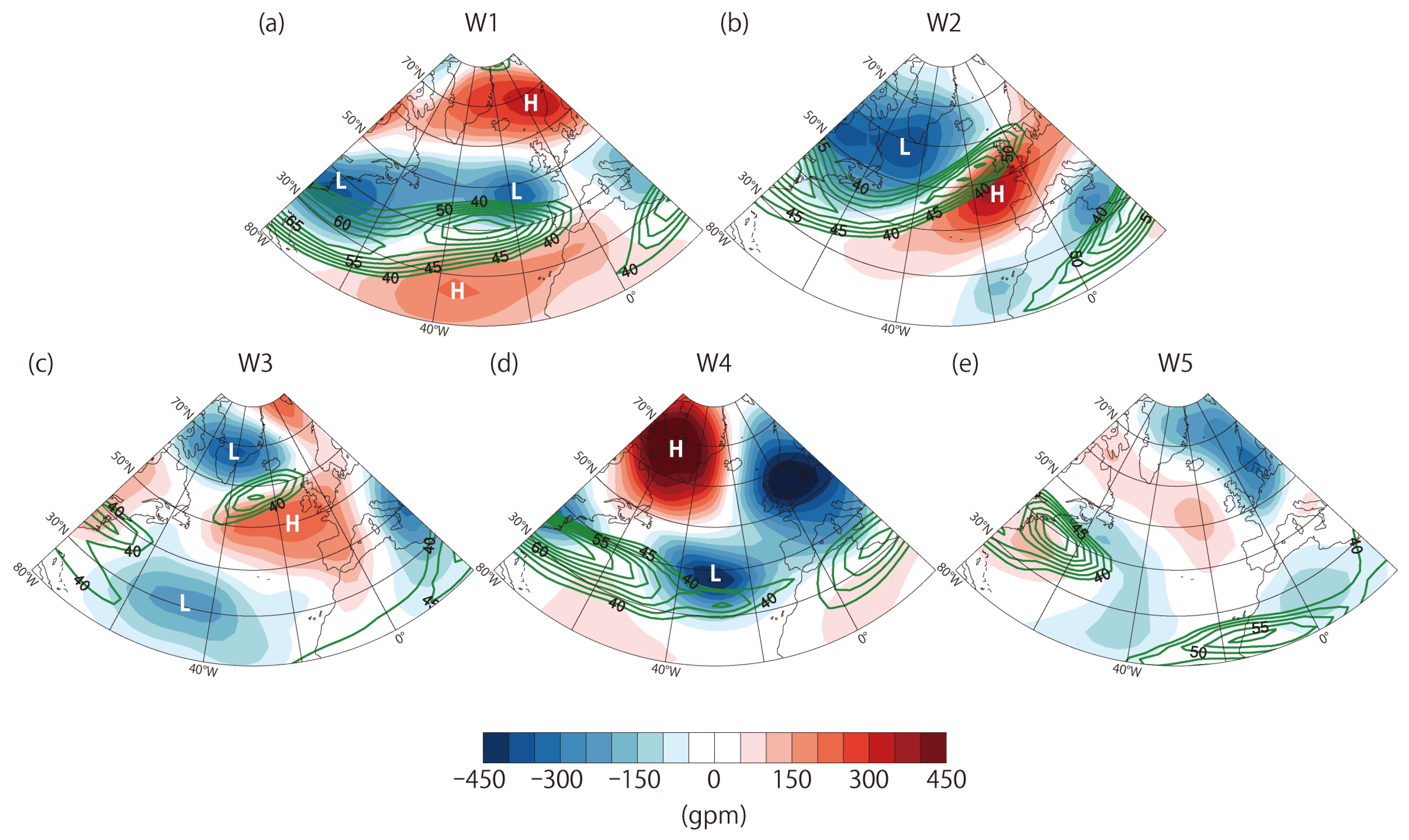
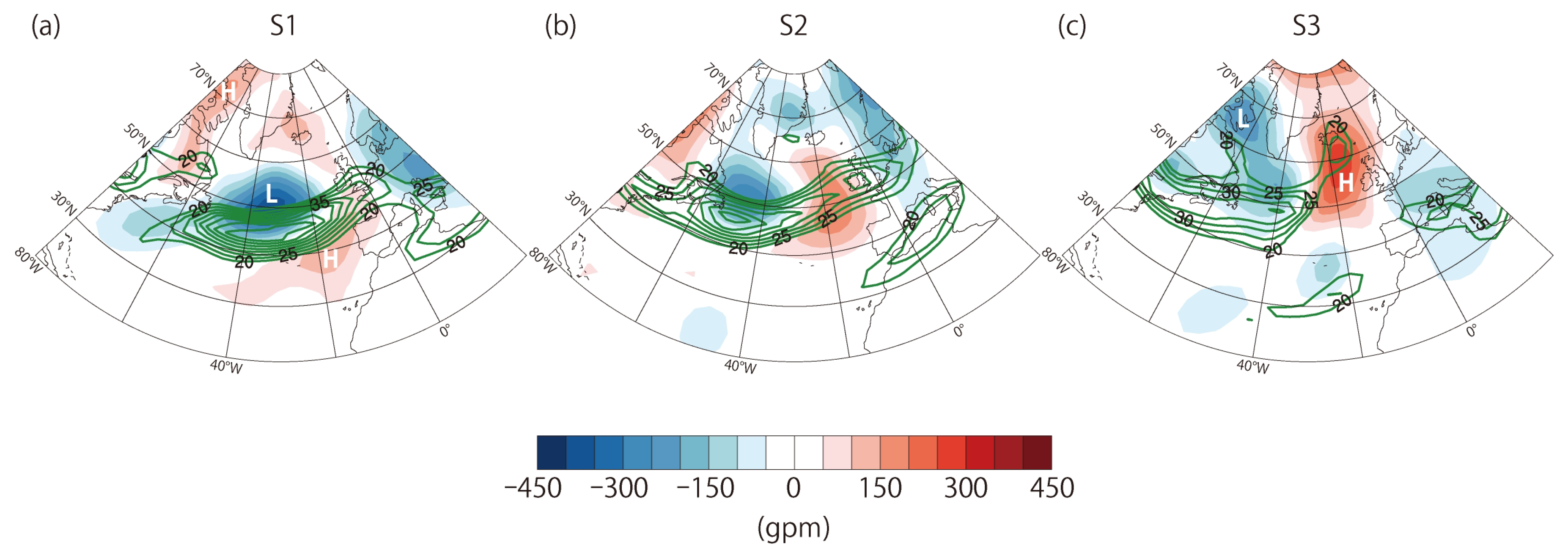
2.1. Weather Pattern Analysis

Weather patterns over the North Atlantic were analyzed by using the EMAC model simulations. The EMAC model is a numerical chemistry and climate simulation system which includes submodels describing tropospheric and middle atmosphere processes and their interaction with oceans, land, and influences coming from anthropogenic emissions [24,25]. EMAC is a state-of-the art model that is applied for international model intercomparisons for the World Meteorological Organization/the United Nations Environment Programme Ozone Assessments (Chemistry–Climate Model Initiative project) and the Intergovernmental Panel on Climate Change (Coupled Model Intercomparison Project 6 project) [29]. EMAC comprises the second version of the Modular Earth Submodel System (MESSy2) to link multi-institutional computer codes. The core atmospheric model is the fifth generation European Center Hamburg general circulation model (ECHAM5; [30]). Table 1 lists the simulation setup for the EMAC model. We applied EMAC (ECHAM5 version 5.3.02 and MESSy version 2.54) in the T42L90MA resolution, i.e., with a spherical truncation of T42 (corresponding to a quadratic Gaussian grid of approximately 2.8° by 2.8° in latitude and longitude) and 90 vertical hybrid pressure levels up to 0.01 hPa (middle of the uppermost layer; approximately 80 km). With the resolution, the general weather patterns were well simulated. Thus, the resolution was appropriate for the weather pattern analysis (this point is discussed in Section 3). A ten-year EMAC simulation was carried out for the period from December 2008 to August 2018. The basic namelist setup for the ECHAM5 simulations (referred to the E5 setup, no chemistry) was employed; the EMAC model was nudged towards the realistic meteorology (the European Centre for Medium-Range Weather Forecasts (ECMWF) Reanalysis (ERA-Interim) dataset [31]). Further information about MESSy, including the EMAC model system, is available from the MESSy Consortium Website [32].
The daily variability in the North Atlantic weather patterns was analyzed by the method described by Woollings et al. [33] and Irvine et al. [34]. The ten-year EMAC simulation results were used for the analysis, which provided ten complete winters (December, January and February) and summers (June, July and August). The North Atlantic Oscillation (NAO; [35]) and the East Atlantic (EA; [36]) patterns are the prominent patterns over the North Atlantic in both winter and summer. The NAO pattern consists of a north–south dipole of height anomalies; one center located over Greenland and the other center of the opposite sign located over the central North Atlantic. The EA pattern also consists of a north–south dipole of height anomalies, which is structurally similar to a southward shifted NAO pattern. Diagnostic indices of the NAO and the EA were calculated by considering the similarity of daily mean geopotential height anomalies at 250 hPa to typical NAO and EA teleconnection patterns over the North Atlantic (80° W–0, 30° N–75° N). For the calculation, the threshold values of the NAO and the EA pattern indices were set to 0.4 for winter and to 0.3 for summer, respectively; these thresholds were chosen because Irvine et al. [34] showed that the threshold values enable clearly identifying weather types. Both indices characterize the position and strength of a jet stream, so that all days of the ten complete winters and summers in the EMAC model simulation results are classified into types for winter and for summer. In addition, representative days for each weather type were selected for the following air traffic simulations (the selected days are discussed in detail in Section 3). Those representative days were selected from the consecutive days that were in the same weather type for more than five days. Because the same weather pattern is persistent, this selection procedure ensures that the representative days express obvious features of each weather type over the North Atlantic.

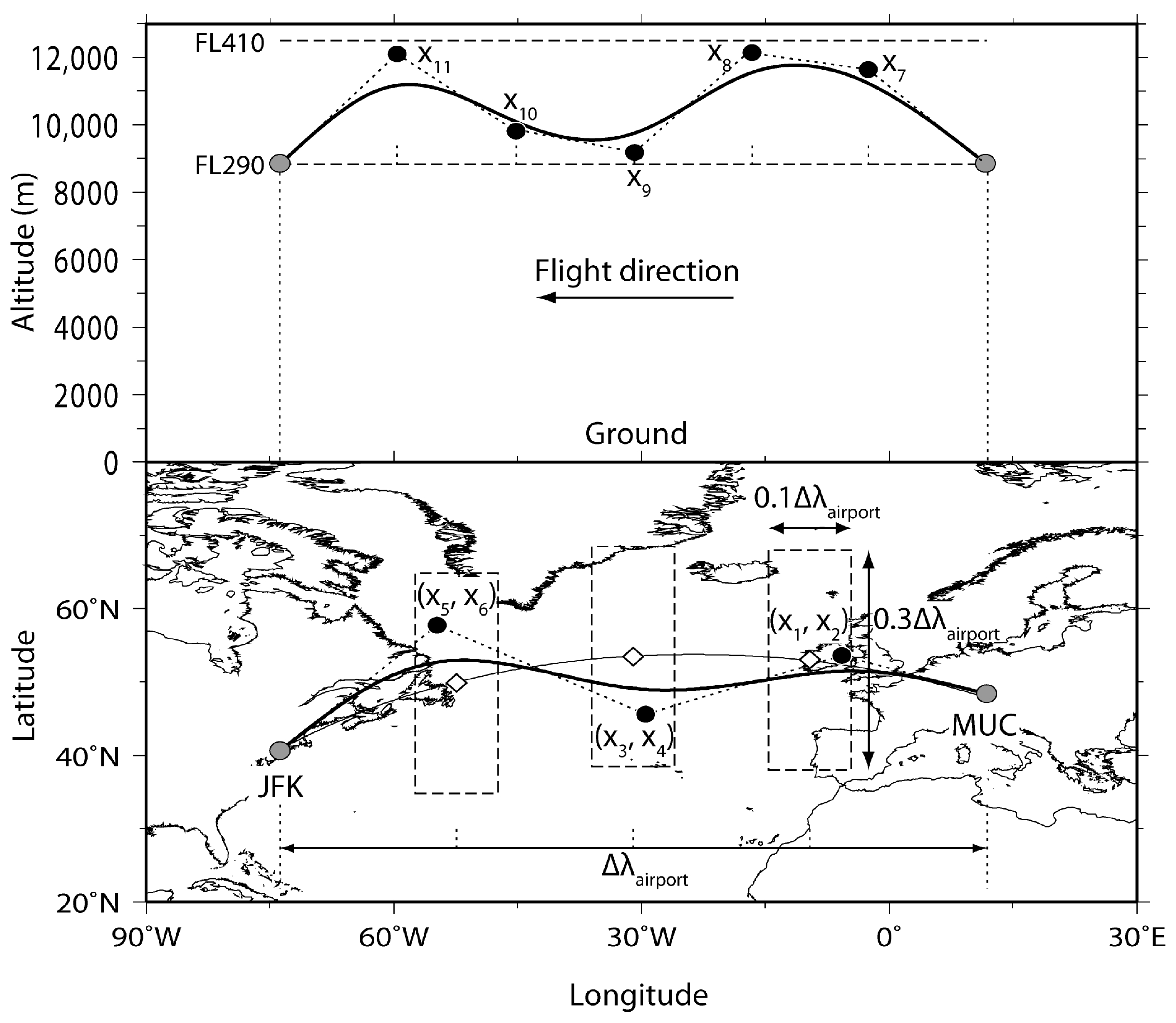
2.2. Air Traffic Simulation

Additional EMAC model simulations were performed for the air traffic simulations utilizing the AirTraf submodel (version 2.0 [28]). AirTraf can simulate global air traffic in the EMAC model with respect to a user-selected aircraft routing strategy (called a routing option) and calculate typical flight characteristics corresponding to the air traffic. AirTraf consists of a total energy model based on the EUROCONTROL’s Base of Aircraft Data (BADA) method [37], the German Aerospace Center (DLR) fuel flow correlation method [38], and the Adaptive Range Multi-Objective Genetic Algorithm (ARMOGA version 1.2.0 [39,40,41]). The total energy model describes the aircraft’s equations of motion based on the assumption of a point-mass model and equates the rate of work performed by forces acting on the aircraft to the rate of increase in potential and kinetic energy. The combination of the total energy model and the DLR fuel flow correlation method enables the calculations of fuel use, NOx and H2O emissions, etc., under actual flight conditions. ARMOGA is a stochastic optimization algorithm and executes the flight trajectory optimization. Once a one-day flight plan including multiple flights is obtained, AirTraf optimizes three-dimensional flight trajectories according to a selected aircraft routing option for every airport pair under weather conditions at the departure time of the respective flights on a target day (the method of the flight trajectory optimization is described in Appendix A). For the air traffic simulations, the aforementioned setup for the EMAC model (Table 1) was employed; the additional setup for the AirTraf submodel is listed in Table 2. The simulation period was changed for the air traffic simulations: one-day simulations were carried out for five aircraft routing options with 103 North Atlantic flights for the representative days which were determined from the weather pattern analysis (see Section 3). The five routing options are as follows: flight time, fuel use, COC [13], contrail formation, and climate impact (we will abbreviate the options to, e.g., the “climate option” here). These options represent the objects to be minimized; that is, an objective function f is defined for a selected routing option, and a single-objective flight trajectory optimization problem is solved: Minimize f. The optimization setup listed in Table 2 was determined by the benchmark tests [27].
The AirTraf submodel has some limitations: AirTraf only considers a cruise flight phase, because the proportion of other flight phases, such as take-off and landing, to the cruise flight phase is small for North Atlantic flights, and the optimization flexibility is limited in the other flight phases. In addition, trajectory conflicts and air traffic management (operating constraints [42]) are neglected. For further details on the limitations, we refer the reader to Yamashita et al. [27].

2.3. Formulations of Objective Functions for the COC, Contrail and Climate Routing Options

The specific objective functions for the COC, the contrail and the climate options were integrated in AirTraf 2.0. Thus, the formulations of those functions are described in the following sections.

2.3.1. COC

The COC option minimizes the airline operating costs indicated by COC [13], which is commonly used as a criterion for airline economics and includes the cost element for flight crew, cabin crew, landing fee, navigation fee, fuel, and maintenance for both airframe and engines (no costs for depreciation, insurance, and interest are included). The objective function is formulated as follows:
f = C O C = C f l i g h t c r e w + C c a b i n c r e w + C l a n d i n g + C n a v i g a t i o n + C f u e l + C a i r f r a m e + C e n g i n e ,
where C denotes a cost in USD; Equation (1) becomes a function of flight time and fuel. For further details on the COC calculation method, we refer the reader to Liebeck et al. [13].

2.3.2. Contrail Formation

Yin et al. [46] developed the contrail option to prevent contrail formations by using the submodel CONTRAIL (version 1.0 [47]). This option minimizes the total contrail distance in km(contrail) of a flight. The contrail distance is defined as the potential persistent contrail cirrus coverage [48,49] (fraction of an EMAC grid box which is maximally covered by contrails) multiplied by a flight distance in km. The objective function can be written as follows:
f = i = 1 n w p 1 P C C d i s t , i = 10 3 i = 1 n w p 1 ( P o t c o v i d i ) ,
where i is the index for waypoints and flight segments of a flight trajectory, nwp is the number of waypoints (Table 2), PCCdist,i is the contrail distance in km(contrail), Potcovi is the potential persistent contrail cirrus coverage (fraction), and di is the flight distance in m. This objective function is the simple form to only consider the contrail distance, and thus further physical processes such as contrail spreading, changes in contrail coverage area, contrail lifetime, and the contrail radiative forcing are not included.

2.3.3. Climate Impact

The climate option minimizes the anticipated climate impact of a flight, i.e., the average temperature response for the time horizon of 20 years (ATR20total) in Kelvin by using the submodel ACCF (version 1.0). The submodel ACCF consists of algorithmic climate change functions (aCCFs; for references, see below). The aCCFs are approximation functions based on regression analyses for the CCF dataset which was obtained from detailed EMAC model simulations including radiative impacts [47,50]; the CCF dataset for contrails was exceptionally obtained from contrail radiative forcing calculations based on the ERA-Interim dataset [31] and contrail trajectory data (Yin et al., (manuscript in preparation, 2021)). The aCCFs represent a correlation of meteorological variables at the time of flight with the anticipated climate impacts. The aCCFs values of ozone (in K(kg(NO2))−1), methane (in K(kg(NO2))−1), water vapor (in K(kg(fuel))−1), CO2 (in K(kg(fuel))−1) and contrails (in K(km(contrail))−1) are calculated online in EMAC by the submodel ACCF, and then the corresponding five ATR20s (in K) are calculated by
A T R 20 O 3 , i = a C C F O 3 , i × N O x , i × 10 3 ,
A T R 20 C H 4 , i = a C C F C H 4 , i × N O x , i × 10 3 ,
A T R 20 H 2 O , i = a C C F H 2 O , i × F U E L i ,
A T R 20 C O 2 , i = a C C F C O 2 × F U E L i ,
A T R 20 c o n t r a i l , i = a C C F c o n t r a i l , i × P C C d i s t , i ,
where NOx,i is the NOx emissions (in g(NOx)), and FUELi is the fuel use (in kg(fuel)). The derivation and validation of the aCCFs of ozone, methane, and water vapor have been published by Van Manen [51], Yin et al. [52], and Van Manen and Grewe [53]; the aCCF of contrails is described by Yin et al. (manuscript in preparation, 2021). Here, we mention the climate impact of contrails. In general, contrails warm the Earth atmosphere by reducing the outgoing terrestrial (longwave) radiation and could cool the Earth atmosphere by reflecting part of the solar (shortwave) radiation. The nighttime contrails always have a warming effect because of no solar radiation, whereas the daytime contrails can have a warming and cooling effects. The aCCFcontrail considers those nighttime and daytime contrail effects, depending on Potcov, the temperature, the outgoing longwave radiation, local time, the time of sunrise, and solar zenith angle. Thus, ATR20contrail can take positive and negative values. Finally, the objective function can be written by combining the five ATR20s into ATR20total as follows:
A T R 20 t o t a l , i = A T R 20 O 3 , i + A T R 20 C H 4 , i + A T R 20 H 2 O , i + A T R 20 C O 2 , i + A T R 20 c o n t r a i l , i ,
f = i = 1 n w p 1 A T R 20 t o t a l ,   i .

3. Characteristics of North Atlantic Weather Patterns

Table 3 summarizes the obtained North Atlantic weather types and their characteristics. Both the NAO and the EA indices successfully classified the days of the ten complete winters and summers into five types for winter (referred to as types W1–W5) and into three types for summer (referred to as types S1–S3). In the second column, the positive values of the NAO/EA indices indicate that the anomaly fields have the same structure as the typical teleconnection pattern, whereas their negative values indicate that the anomaly fields have the same structure of the opposite sign. In addition, the weather types are clearly characterized by the position and strength of a jet stream, and the representative days of those types are determined well.
To validate our weather pattern analysis, the frequency for each of the weather types was examined by counting the number of days of the ten complete winters and summers for which each type occurs. Table 3 shows that types W1–W4 occur on average 14.7–18.9 days per winter, and type W5 occurs most frequently on average 22 days per winter. In summer, types S1 and S3 occur with similar frequency, on average 26 and 22.9 days per summer, respectively; and type S2 occurs most frequently, on average 43.1 days per summer. Irvine et al. [34] similarly analyzed the daily variability in the North Atlantic weather patterns by using the ERA-Interim dataset [31] from 1989 to 2010, which provided 21 complete winters and summers. They reported that types W1–W4 average to 15–19 days per winter and type W5 occurs most frequently (26 days per winter). In summer, types S1 and S3 average to 19 and 18 days per summer, respectively; and type S2 occurs most frequently (55 days per summer). The frequencies obtained from our results agree with those shown by Irvine et al. [34], which corroborates the validity of our analysis.
The characteristics of the individual weather types are described briefly. Figure 1 and Figure 2 show the daily mean geopotential height anomaly and zonal wind speed at 250 hPa for the representative days of each weather type in winter and summer. For type W1 (Figure 1a), the anomaly resembles the positive phase of the EA pattern (EA+), where blocking over central western Europe occurs and the strong central jet stream exists. The anomaly of type W2 (Figure 1b) resembles the positive phase of the NAO pattern (NAO+), where the jet stream tilts meridionally to the north. When type W3 (Figure 1c) is observed, the anomaly resembles the negative phase of the EA pattern (EA−). The anomaly actually shows a similar structure to type W1 (EA+); however, it is opposite in sign to type W1. EA− reflects the occurrence of blocking over southwest Europe, which diverts the jet stream to the north. As a result, the jet stream becomes weak and tilts southwest–northeast. For type W4 (Figure 1d), the anomaly is similar to the negative phase of the NAO pattern (NAO−), which is associated with the occurrence of high-latitude blocking over Greenland [33,54] and southern shifts of the jet stream. The strong zonally oriented jet stream is confined over the east coast of the U.S. Type W5 (Figure 1e), which has little similarity to the NAO and EA patterns. The jet stream is confined over the east coast of the U.S. and is relatively weak. In contrast to winter, Figure 2 shows that the variability in the jet stream position becomes small and the strength of the jet stream reduces in summer. With the present pattern analysis method [33,34], the weather patterns are classified into three types (Table 3). Type S1 (Figure 2a) resembles EA+, where the strong zonal jet stream exists. By comparing type S1 (Figure 2a) with type W1 (Figure 1a), their anomalies show the similar structure of EA+; however, the magnitude of the anomaly of type S1 and the magnitude of the wind speed of type S1 are less than those of type W1. Type S2 (Figure 2b) has little similarity to the EA pattern and shows slight north shifts of the jet stream. Type S3 (Figure 2c) corresponds to EA−, where the weaker jet stream tilts southwest–northeast.

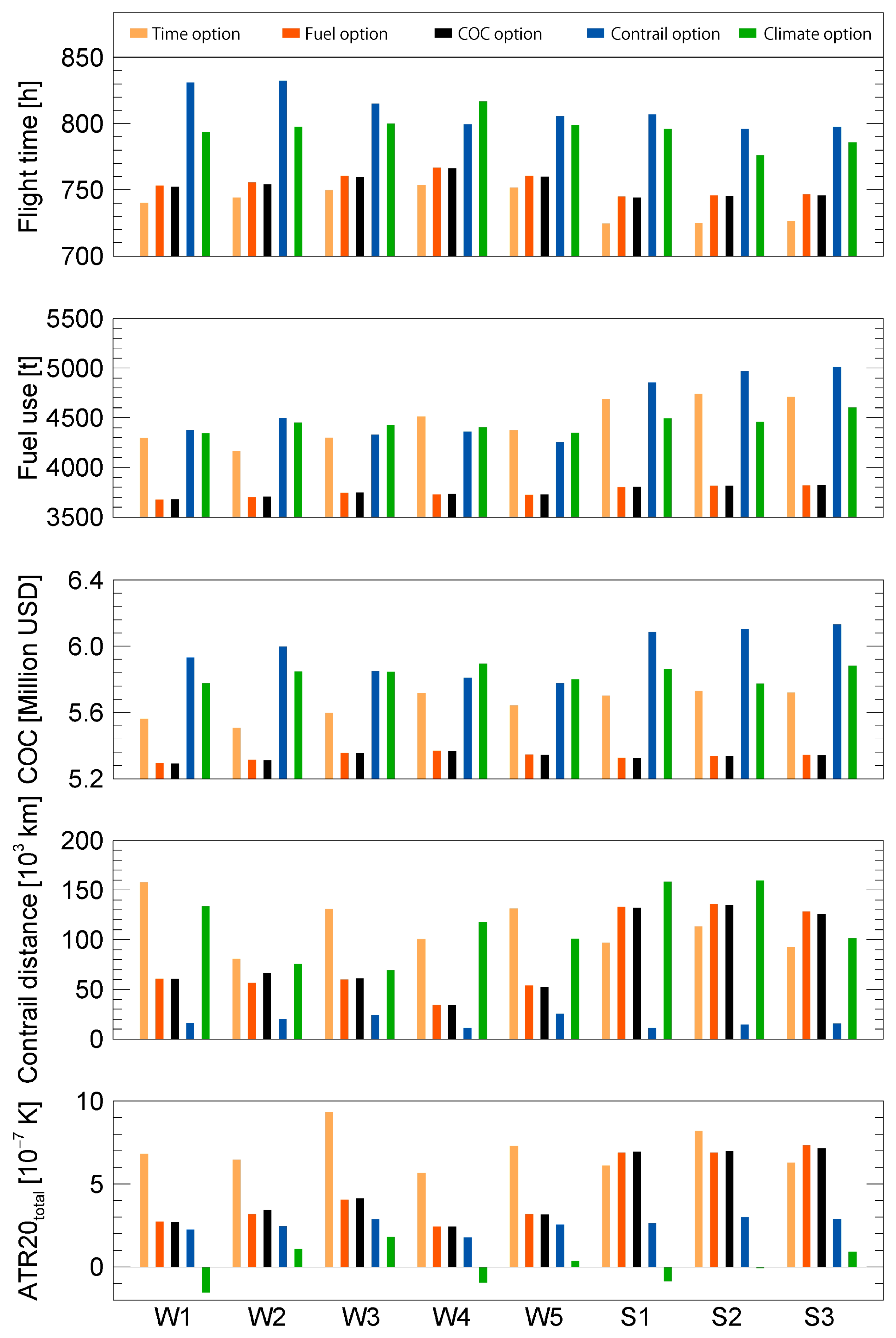
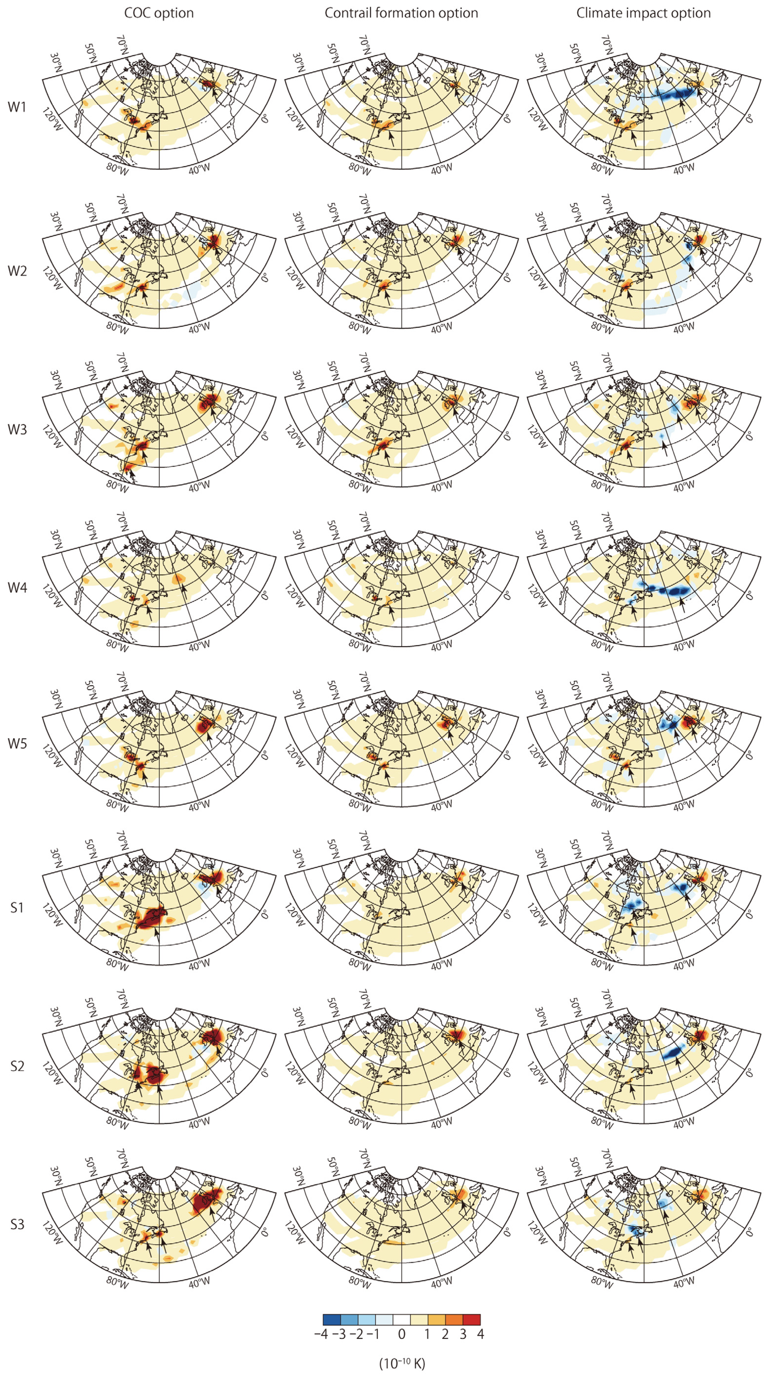
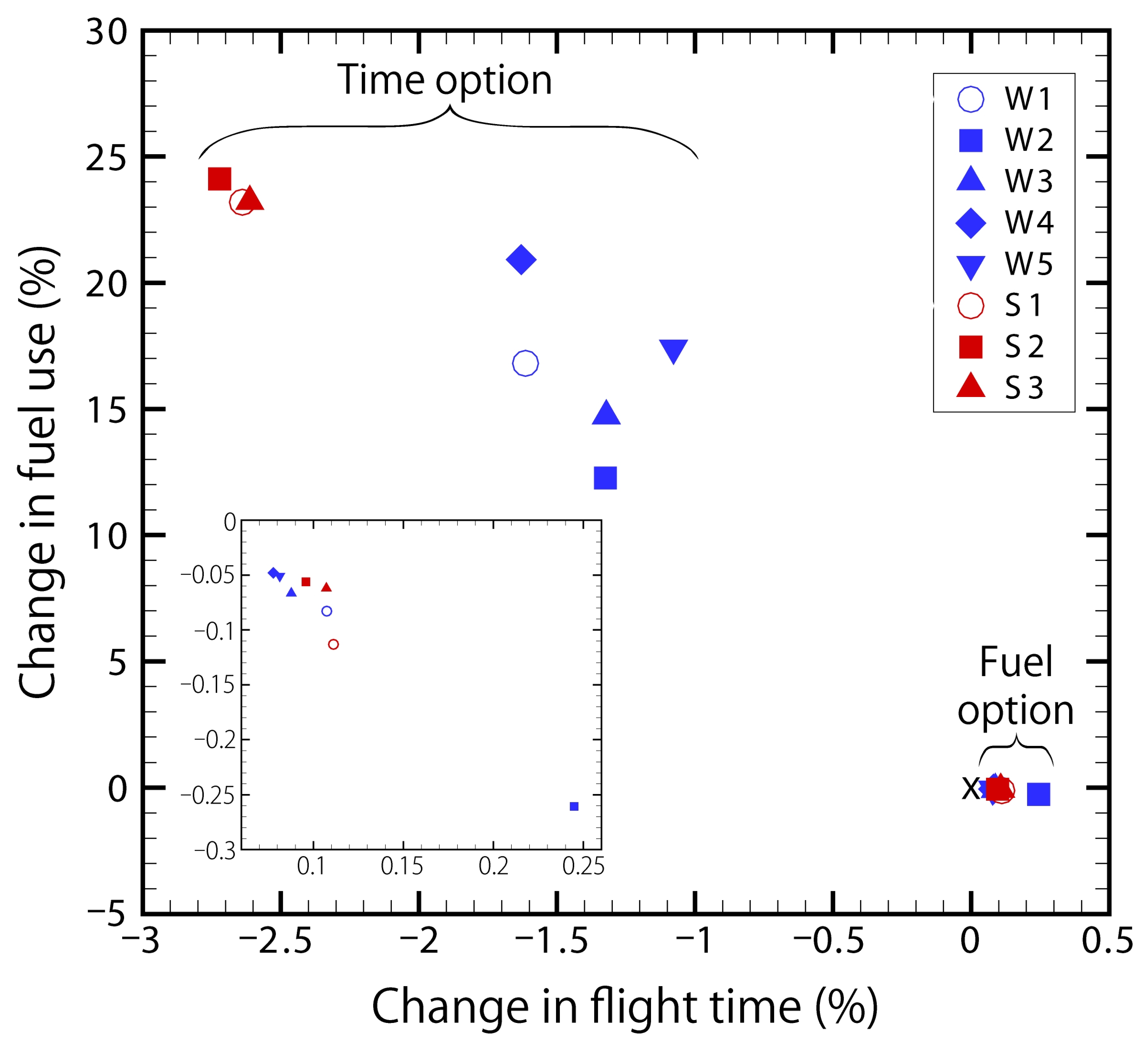
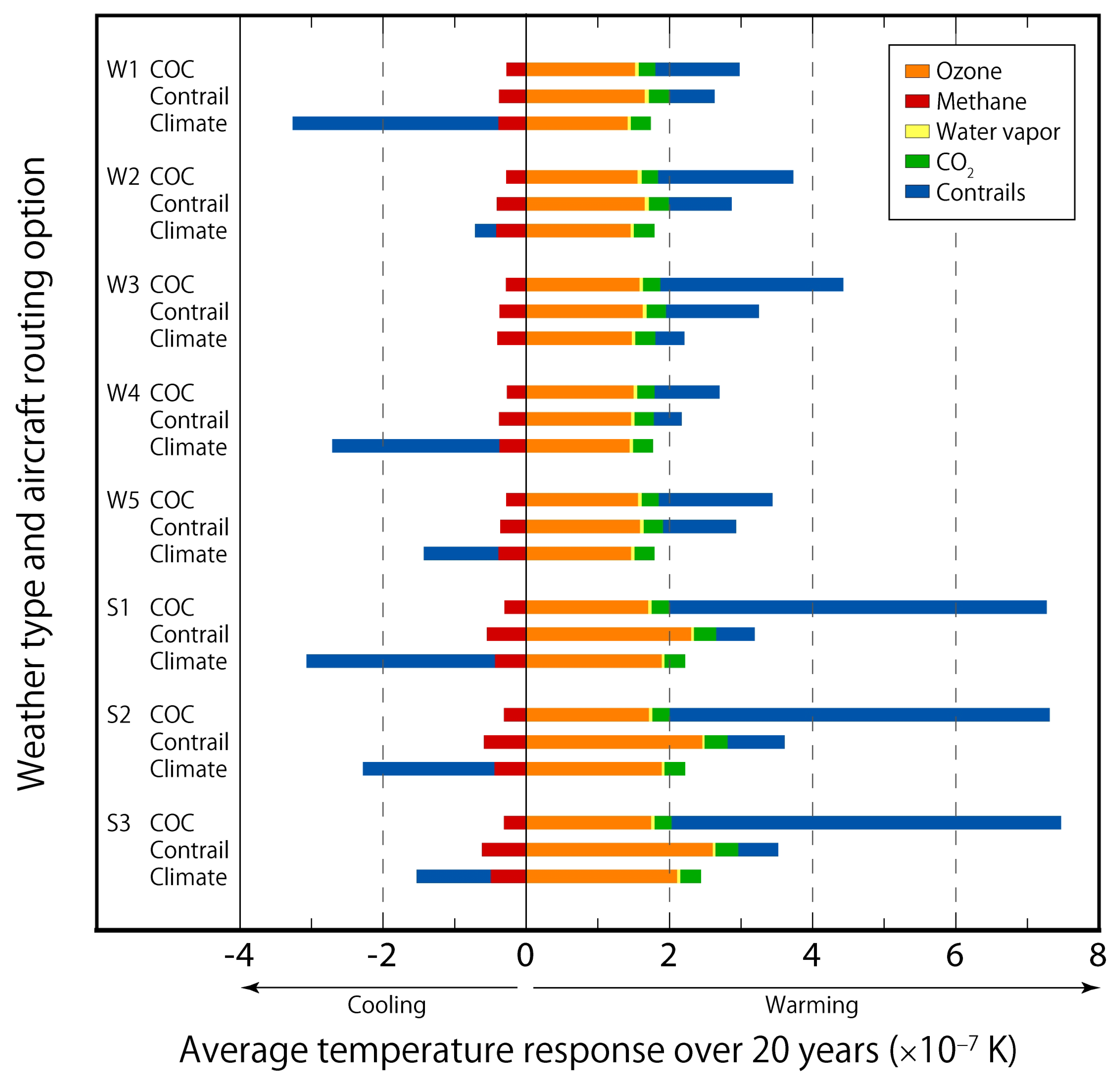
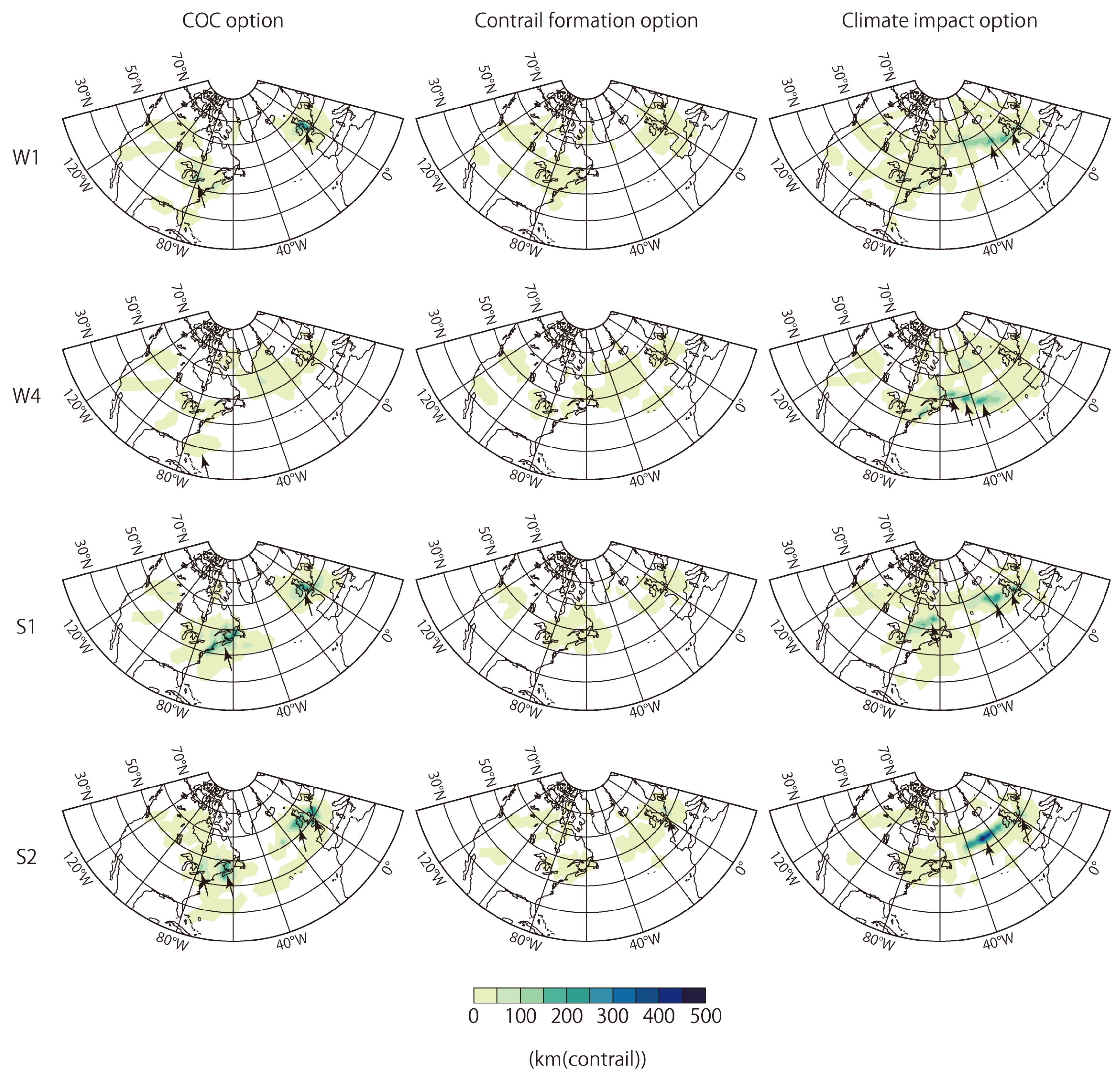
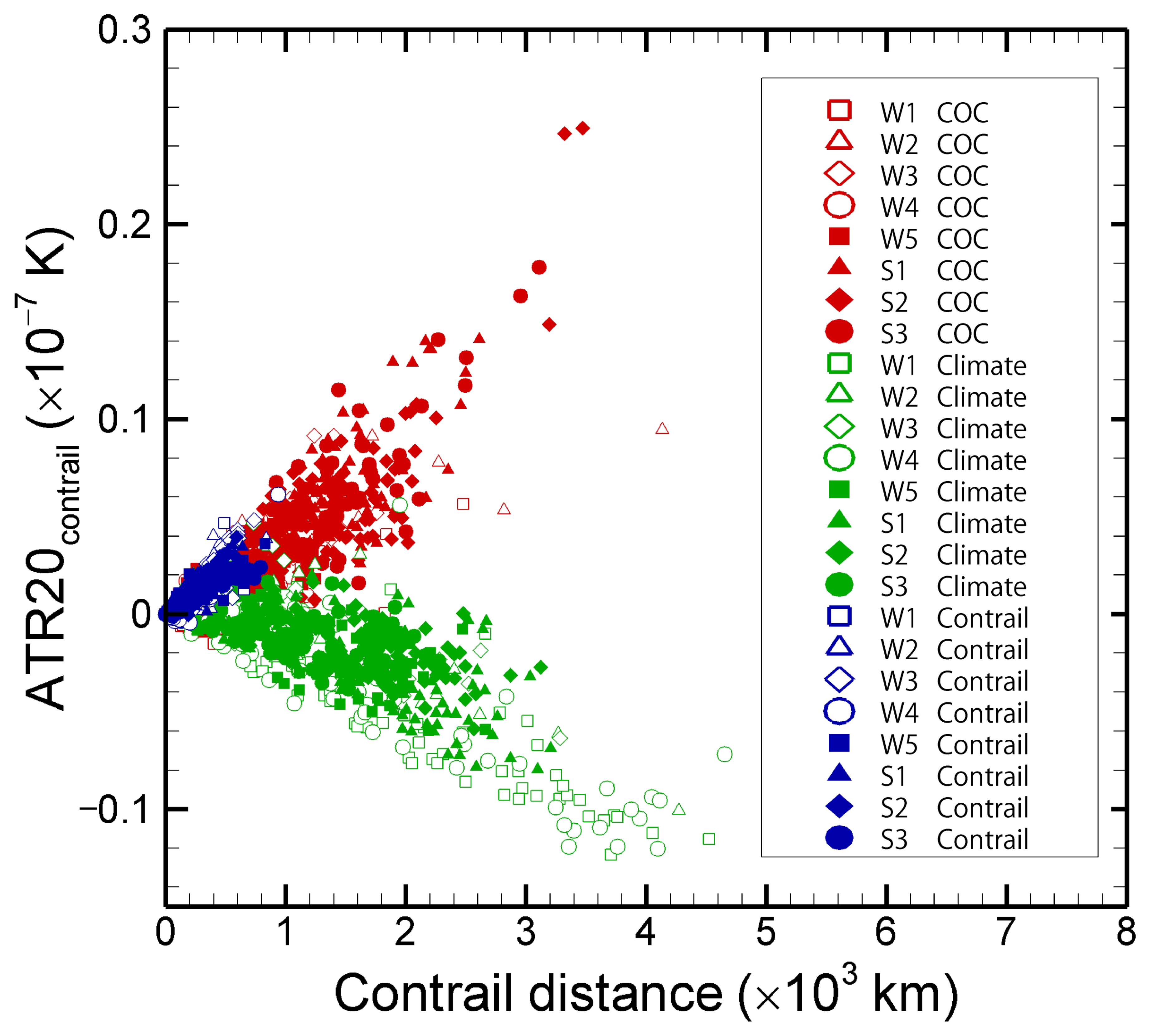
4. Characteristics of North Atlantic Aircraft Routing Strategies

The one-day air traffic simulation results obtained with the five aircraft routing options were analyzed and some aircraft routing characteristics that are common to all the representative days were examined. Figure 3 shows the flight characteristics of the one-day air traffic (total 103 flights) for the five routing options for easy comparison. Here, we focus on relative changes (in %) in the flight characteristics to those obtained by the COC option, because the COC option can be considered the current aircraft routing strategy (baseline in our analysis).
First, the COC and the climate options are analyzed. Of the five routing options, the COC option successfully achieves the lowest COC for all the weather types in winter and summer (Figure 3), whereas the climate option successfully achieves the lowest ATR20total for all the weather types. Figure 4 shows a comparison of the climate impact (ATR20total) for the respective weather types in winter and summer; for each weather type, ATR20total for the COC, the contrail and the climate options are shown. A comparison of Figure 4 (left) with Figure 4 (right) indicates that the climate option decreases the positive values of ATR20total (i.e., warming effects) over northwest Europe and over the east coast of the U.S. In addition, the climate option produces regionally negative values of ATR20total (i.e., cooling effects) near Iceland and near Greenland, and over the North Atlantic Ocean, over eastern Canada and over the east coast of the U.S. The decreasing warming effects and the increasing cooling effects result in decreased ATR20total by 56.5 (type W3) to 156.3% (type W1; this point is discussed in detail below); however, the climate option increases the COC significantly. The climate option yields the highest COC for types W4 and W5 and yields the second highest COC for the other weather types (Figure 3). The increasing COC ranges from 8.2 (type S2) to 10.1% (types W2, S1 and S3). A clear trade-off exists between the cost and the climate impact, and the trade-off is observed for all the weather types in winter and summer.
The next analysis focuses on the time, the fuel and the COC options. Of the five routing options, the time option achieves the shortest flight time and the fuel option achieves the lowest fuel use for all the weather types (Figure 3). To minimize COC, a reduction in both flight time and fuel use is desirable, because COC depends on the two factors [13]; however, a trade-off exists between the flight time and the fuel use. Figure 5 shows the relative changes in flight time and fuel use among the time, the fuel and the COC options. For the time option, the benefit in flight time reduction ranges from −2.7 (type S2) to −1.1% (type W5), whereas the fuel penalty of the time option ranges from 12.3 (type W2) to 24.1% (type S2). In contrast, for the fuel option, the benefit in fuel use reduction ranges from –0.3 (type W2) to −0.05% (type W5), whereas the time penalty of the fuel option ranges from 0.08 (type W5) to 0.24% (type W2). The COC option requires more flight time and consumes less fuel than those of the time option; the COC option consumes more fuel and requires less flight time than those of the fuel option. The COC option lies between the time and the fuel options and yields the best compromise between the flight time and the fuel use, which enables minimizing COC for all the weather types. The COC option shows similar values of flight time and fuel use to the fuel option; however, the small difference in the two factors enables the further cost reduction of USD 0.001–0.002 million per day (per 103 flights) from flying with the fuel option (for type S1, the cost reduction is USD 0.0008 million).
The contrail option successfully achieves the shortest contrail distance for all the weather types (Figure 3), which results in a reduction in contrail distance by 51 (type W5) to 92% (type S1) over that of the COC option. In addition, the contrail option significantly reduces ATR20total. A comparison of Figure 4 (left) with Figure 4 (center) indicates that the contrail option decreases the positive values of ATR20total over northwest Europe, over the east coast of the U.S. and over the North Atlantic Ocean. Of the five routing options, the contrail option achieves the second lowest ATR20total for all the weather types, which results in decreased ATR20total by 16.7 (type W1) to 62.1% (type S1); however, as with the climate option, the contrail option increases COC. The contrail option yields the highest COC for types W1 to W3 and S1 to S3 and yields the second highest COC for types W4 and W5. The increasing COC ranges from 8.1 (type W5) to 14.8% (type S3).
Our results indicate that the contrail and the climate options are effective to reduce the climate impact of ATR20total. Interestingly, those two options take different approaches to reduce ATR20total. Figure 3 shows that the contrail option takes positive values of ATR20total (warming effects) for all the weather types, whereas the climate option yields negative values of ATR20total (cooling effects) for types W1, W4, S1 and S2. To examine the difference in the sign of ATR20total, Figure 6 compares the five components of ATR20total for the COC, the contrail and the climate options. Obviously, the key component is ATR20contrail, which strongly affects the values of ATR20total. The contrail option reduces the warming effect of contrails for all weather types, whereas the climate option reduces the warming effect of contrails for type W3 and yields the cooling effect of contrails for other types. To understand the effects of both options intuitively, Figure 7 shows a comparison of the contrail distance for types W1, W4, S1 and S2; for each weather type, the contrail distance for the COC, the contrail and the climate options are compared. A comparison of Figure 7 (left) with Figure 7 (center) shows that the contrail option decreases the contrail formations near Greenland (type W4), over northwest Europe (types W1, S1 and S2), and over the east coast of the U.S. (types W4, S1 and S2), where the positive values of ATR20total decrease (see Figure 4 (center)). A comparison of Figure 7 (left) with Figure 7 (right) shows that the climate option decreases the contrail formations over northwest Europe (types W1, S1 and S2) and over the east coast of the U.S. (types S1 and S2), where the positive values of ATR20total decrease (see Figure 4 (right)). In addition, the climate option increases the contrail formations near Iceland (types W1, S1 and S2), over the North Atlantic Ocean (type W4), and over eastern Canada (type S1), where the negative values of ATR20total increase (see Figure 4 (right)). Moreover, Figure 8 plots the contrail distance vs. ATR20contrail for individual flights for all the weather types. We see that the contrail option significantly decreases the contrail distance (the contrail option achieves the shortest contrail distance for all the weather types, as shown in Figure 3) and shows the positive values of ATR20contrail for almost all flights. On the other hand, the climate option has longer contrail distances than those of the contrail option and shows the negative values of ATR20contrail for many flights. The results indicate that the contrail option minimizes the overall contrail formations at all times, thereby reducing the positive ATR20contrail. The reducing ATR20contrail results in the second lowest ATR20total for all weather types; however, the values of ATR20total are all positive (warming effects; see Figure 3). In contrast, the climate option reduces warming contrails during the day and night, and actively forms cooling contrails during the day, which leads to decreased positive ATR20contrail for type W3 and to the negative values of ATR20contrail for the other types (Figure 6). The decreasing ATR20contrail results in the lowest ATR20total for all the weather types and in particular, in the negative values of ATR20total for types W1, W4, S1 and S2 (Figure 3).

5. Discussion

In this study, EMAC/AirTraf was only applied to the selected representative days because of the high computational demands of the flight trajectory optimization. Although the aircraft routing characteristics shown here agree with those reported by previous studies introduced in Section 1, our findings are still limited to the weather conditions of those representative days. To generalize those characteristics of aircraft routing strategies, statistical analyses are required on the basis of a large number of air traffic simulations with different routing options for many days and seasons. A follow-up study will focus on the extension of the simulation dataset and on a statistical interpretation. In addition, our results show some trends of the seasonal variation in flight characteristics; for example, the COC option shows larger contrail distances in summer than those in winter, and thus this option has larger values of ATR20total in summer (see Figure 3 and Figure 6). This emphasizes the efficient reduction in contrail formation by selecting the contrail option in summer. Figure 5 also shows that the overall benefit in flight time caused by the time option increases in summer, although the jet stream is strong over the North Atlantic in winter, as shown in Figure 1. The statistical analyses will reveal the relationship between the aircraft routing characteristics and weather conditions, including seasonal variations in flight characteristics.
Last but not least, the five aircraft routing options used in this study can be employed to perform air traffic simulations for multi-criteria aircraft routing strategies [8]. We extend the present optimization method to solve multi-objective optimization problems among different aircraft routing options, find a set of trade-off solutions (optimal flight trajectories), and then choose one flight trajectory from the obtained set of trade-off solutions based on higher-level information, such as various subjective and problem-dependent considerations. If we consider two conflicting objectives of flight trajectory optimization, i.e., the minimization of cost and minimization of climate impact, the extension of the present optimization method enables finding an eco-efficient aircraft trajectory which shows a substantial reduction in climate impact and a small increase in costs. This feature allows one to perform air traffic simulations for an eco-efficient aircraft routing strategy.

6. Conclusions

We performed the ten years EMAC model simulation from December 2008 to August 2018 in the specified dynamics mode nudging with ERA-Interim reanalysis dataset. The daily variability in the North Atlantic weather patterns was analyzed on the basis of the similarity of daily-mean geopotential height anomalies at 250 hPa to typical NAO and EA teleconnection patterns. All days of the ten complete winters and summers in the EMAC simulation were successfully classified into commonly occurring weather types, i.e., five weather types for winter (types W1 to W5) and three types for summer (types S1 to S3). The weather types were clearly characterized by the position and strength of the jet stream at 250 hPa over the North Atlantic. The obtained frequency of each of the weather types was compared with the literature data, and the validity of our analysis was confirmed. The representative days for each weather type were selected and a total of 103 North Atlantic flights of an Airbus A330 aircraft were simulated with the five aircraft routing options for each representative day by using the EMAC model with the AirTraf submodel. The variation in flight characteristics among those routing options was analyzed, and some characteristics of the aircraft routings were examined. The results show that the climate option reduces ATR20total the most and shows a trade-off between the COC and ATR20total; the COC option lies between the time and the fuel options and achieves the lowest COC by taking the best compromise between the flight time and the fuel use. The contrail option shows the second lowest ATR20total, which causes an increase in COC. These characteristics are common to the representative days of each weather type over the North Atlantic. We extend our methodology to long-term simulations and statistically analyze the obtained dataset, which could clarify the relationship between the aircraft routing characteristics and weather conditions. The present optimization method is also extended so that AirTraf can simulate air traffic for multi-criteria aircraft routing strategies.

Author Contributions

Conceptualization, H.Y., V.G. and S.M.; method and software, H.Y., F.Y., V.G., P.J., S.M., B.K., K.D. and C.F.; investigation, H.Y.; resources, C.F. and S.M.; writing—original draft preparation, H.Y.; writing—review and editing, H.Y., F.Y. and P.J.; visualization, H.Y.; project administration and funding acquisition, V.G. and S.M. All authors have read and agreed to the published version of the manuscript.

Funding

This study was funded by the DLR project Eco2Fly (2018–2022).

Institutional Review Board Statement

Not applicable.

Informed Consent Statement

Not applicable.

Data Availability Statement

AirTraf is implemented as a submodel of the Modular Earth Submodel System (MESSy). MESSy is being continuously developed and applied by a consortium of institutions. The usage of MESSy and access to the source code are licensed to all affiliates of institutions which are members of the MESSy Consortium. Institutions can become a member of the MESSy Consortium by signing the MESSy Memorandum of Understanding. More information can be found on the MESSy Consortium website (http://www.messy-interface.org). The submodel AirTraf 2.0 has been available since the official release of MESSy version 2.54. The status information for AirTraf including the license conditions is available on the website. The data from the simulations will be provided by the authors on request.

Acknowledgments

The flight plan was provided by the European Union FP7 project REACT4C (Reducing Emissions from Aviation by Changing Trajectories for the Benefit of Climate; grant ACP8-GA-2009-233772; https://www.react4c.eu/). We gratefully acknowledge the computational resources for the simulations which were provided by the German Climate Computing Center (the Deutsches Klimarechenzentrum DKRZ). We wish to acknowledge our colleagues, especially Robert Sausen, for his support of the project. We would like to thank Björn Brötz for providing an internal review. We would like to express our gratitude to four anonymous reviewers for their helpful comments and discussion.

Conflicts of Interest

The authors declare no conflict of interest.

Appendix A. Formulation of Flight Trajectory Optimization

A flight trajectory was optimized with the methods described by Yamashita et al. [27,28]. Figure A1 (adapted from [27]) shows the geometry definition of a flight trajectory from Munich (MUC) to New York (JFK) as an example. Six design variables from x1 to x6 were used for the location (Figure A1, bottom). x1, x3 and x5 indicate longitudes, and x2, x4 and x6 indicate latitudes. Given the geographic locations of an airport pair according to a flight plan, the great circle is calculated between the airports, and central points of three rectangular domains (diamonds) are calculated on the great circle. These points divide the longitude distance between the airports (∆λairport) into four equal parts. The three rectangular domains (0.1∆λairport × 0.3∆λairport) centered at the central points are created for the lower/upper bounds of the six design variables. The coordinates of three control points (CPs, closed circles) are determined: CP1 (x1, x2), CP2 (x3, x4) and CP3 (x5, x6). A flight trajectory is represented by a B-spline curve (third order) with the three CPs, and then waypoints are generated along the trajectory. The altitudes of the airport pair are fixed at FL290 (≈ 8.8 km) and five design variables of x7 to x11 are used to indicate altitudes (Figure A1, top). The longitude coordinates of the five design variables are calculated to divide ∆λairport into six equal parts; the lower/upper bounds of the five design variables are set as [FL290, FL410] (≈ [8.8, 12.5] km). The coordinates of five CPs are determined: CP4 (x7), CP5 (x8), CP6 (x9), CP7 (x10), and CP8 (x11). A flight trajectory is represented by another B-spline curve (third-order) with the five CPs, and then waypoints are generated along the trajectory in such a way that the longitude of the waypoints is the same as that for the flight trajectory on location. As a result, 11 design variables are used to define a whole flight trajectory. ARMOGA [39,40,41] seeks an optimal solution (i.e., flight trajectory) of a single-objective flight trajectory optimization problem with the optimization setup listed in Table 2; the obtained flight trajectory minimizes an objective function corresponding to a selected aircraft routing option. Any arbitrary number of flight plans is applicable to AirTraf simulations and this flight trajectory optimization is executed for every airport pair. The present optimization method can be extended to solve multi-objective optimization problems among different aircraft routing options (see Section 5).
Figure A1. Geometry definition of the flight trajectory in the vertical cross section (top) and projection on the Earth (bottom) [27]. The bold solid line indicates a flight trajectory from Munich (MUC) to New York (JFK). Control points (closed circles) are determined by 11 design variables. Bottom: the dashed boxes show rectangular domains for the lower/upper variable bounds of the six design variables (x1 to x6). Central points (diamonds) of the domains are calculated on the great circle (thin solid line). Top: the dashed lines show the lower/upper variable bounds of the five design variables (x7 to x11).
Aerospace 08 00033 g0a1

References

  1. Skeie, R.B.; Fuglestvedt, J.; Berntsen, T.; Lund, M.T.; Myhre, G.; Rypdal, K. Global temperature change from the transport sectors: Historical development and future scenarios. Atmos. Environ. 2009, 43, 6260–6270. [Google Scholar] [CrossRef]
  2. Lee, D.; Fahey, D.W.; Forster, P.M.; Newton, P.J.; Wit, R.C.N.; Lim, L.L.; Owen, B.; Sausen, R. Aviation and global climate change in the 21st century. Atmos. Environ. 2009, 43, 3520–3537. [Google Scholar] [CrossRef] [PubMed] [Green Version]
  3. Lee, D.; Pitari, G.; Grewe, V.; Gierens, K.; Penner, J.; Petzold, A.; Prather, M.; Schumann, U.; Bais, A.; Berntsen, T. Transport impacts on atmosphere and climate: Aviation. Atmos. Environ. 2010, 44, 4678–4734. [Google Scholar] [CrossRef] [PubMed] [Green Version]
  4. Brasseur, G.P.; Gupta, M.; Anderson, B.E.; Balasubramanian, S.; Barrett, S.R.H.; Duda, D.P.; Fleming, G.G.; Forster, P.M.; Fuglestvedt, J.; Gettelman, A.; et al. Impact of Aviation on Climate: FAA’s Aviation Climate Change Research Initiative (ACCRI) Phase II. Bull. Am. Meteorol. Soc. 2016, 97, 561–583. [Google Scholar] [CrossRef] [Green Version]
  5. ICAO’s Annual Report of the Council, the World of Air Transport in 2018. Available online: https://www.icao.int/annual-report-2018/Pages/the-world-of-air-transport-in-2018.aspx (accessed on 23 October 2020).
  6. Grewe, V.; Dahlmann, K.; Flink, J.; Frömming, C.; Ghosh, R.; Gierens, K.; Heller, R.; Hendricks, J.; Jöckel, P.; Kaufmann, S.; et al. Mitigating the Climate Impact from Aviation: Achievements and Results of the DLR WeCare Project. Aerospace 2017, 4, 34. [Google Scholar] [CrossRef]
  7. Grewe, V.; Matthes, S.; Frömming, C.; Brinkop, S.; Jöckel, P.; Gierens, K.; Champougny, T.; Fuglestvedt, J.; Haslerud, A.; Irvine, E.; et al. Feasibility of climate-optimized air traffic routing for trans-Atlantic flights. Environ. Res. Lett. 2017, 12, 034003. [Google Scholar] [CrossRef]
  8. Matthes, S.; Grewe, V.; Dahlmann, K.; Frömming, C.; Irvine, E.; Lim, L.; Linke, F.; Lührs, B.; Owen, B.; Shine, K.P.; et al. A Concept for Multi-Criteria Environmental Assessment of Aircraft Trajectories. Aerospace 2017, 4, 42. [Google Scholar] [CrossRef] [Green Version]
  9. Green, J.E. Future aircraft greener by design? Meteorol. Z. 2005, 14, 583–590. [Google Scholar] [CrossRef]
  10. Grewe, V.; Bock, L.; Burkhardt, U.; Dahlmann, K.; Gierens, K.; Hüttenhofer, L.; Unterstrasser, S.; Rao, A.G.; Bhat, A.; Yin, F.; et al. Assessing the climate impact of the AHEAD multi-fuel blended wing body. Meteorol. Z. 2017, 26, 711–725. [Google Scholar] [CrossRef]
  11. Grewe, V.; Champougny, T.; Matthes, S.; Frömming, C.; Brinkop, S.; Søvde, O.A.; Irvine, E.A.; Halscheidt, L. Reduction of the air traffic’s contribution to climate change: A REACT4C case study. Atmos. Environ. 2014, 94, 616–625. [Google Scholar] [CrossRef] [Green Version]
  12. Lührs, B.; Niklass, M.; Froemming, C.; Grewe, V.; Gollnick, V. Cost-Benefit Assessment of 2D and 3D Climate and Weather Optimized Trajectories. In Proceedings of the 16th AIAA Aviation Technology, Integration, and Operations Conference, Washington, DC, USA, 13–17 June 2016. [Google Scholar]
  13. Liebeck, R.H.; Andrastek, D.A.; Chau, J.; Girvin, R.; Lyon, R.; Rawdon, B.K.; Scott, P.W.; Wright, R.A.; Advanced Subsonic Airplane Design and Economic Studies. NASA CR-195443 1995. pp. 1–31. Available online: https://ntrs.nasa.gov/search.jsp?R=19950017884 (accessed on 23 October 2020).
  14. Ng, H.K.; Sridhar, B.; Chen, N.Y.; Li, J. Three-Dimensional Trajectory Design for Reducing Climate Impact of Trans-Atlantic Flights. In Proceedings of the 14th AIAA Aviation Technology, Integration, and Operations Conference, Atlanta, GA, USA, 16–20 June 2014. [Google Scholar]
  15. Celis, C.; Sethi, V.; Zammit-Mangion, D.; Singh, R.; Pilidis, P.P. Theoretical Optimal Trajectories for Reducing the Environmental Impact of Commercial Aircraft Operations. J. Aerosp. Technol. Manag. 2014, 6, 29–42. [Google Scholar] [CrossRef]
  16. Rosenow, J.; Fricke, H. Flight performance modeling to optimize trajectories. In Proceedings of the Deutscher Luft- und Raumfahrtkongress, Braunschweig, Germany, 13–15 September 2016; Available online: https://www.dglr.de/publikationen/2016/420127.pdf (accessed on 23 October 2020).
  17. Mannstein, H.; Spichtinger, P.; Gierens, K. A note on how to avoid contrail cirrus. Transp. Res. Part D Transp. Environ. 2005, 10, 421–426. [Google Scholar] [CrossRef]
  18. Sridhar, B.; Ng, H.K.; Chen, N.Y. Aircraft Trajectory Optimization and Contrails Avoidance in the Presence of Winds. J. Guid. Control Dyn. 2011, 34, 1577–1584. [Google Scholar] [CrossRef]
  19. Schumann, U.; Graf, K.; Mannstein, H. Potential to reduce the climate impact of aviation by flight level changes. In Proceedings of the 3rd AIAA Atmospheric Space Environments Conference, Honolulu, HI, USA, 27–30 June 2011. [Google Scholar]
  20. Xue, D.; Ng, K.K.; Hsu, L.-T. Multi-Objective Flight Altitude Decision Considering Contrails, Fuel Consumption and Flight Time. Sustainability 2020, 12, 6253. [Google Scholar] [CrossRef]
  21. Irvine, E.; Hoskins, B.J.; Shine, K.P. A simple framework for assessing the trade-off between the climate impact of aviation carbon dioxide emissions and contrails for a single flight. Environ. Res. Lett. 2014, 9, 064021. [Google Scholar] [CrossRef]
  22. Soler, M.; Zou, B.; Hansen, M. Flight Trajectory Design in the Presence of Contrails: Application of a Multiphase Mixed-Integer Optimal Control Approach. Transp. Res. Part C Emerg. Technol. 2014, 48, 172–194. [Google Scholar] [CrossRef]
  23. Rosenow, J.; Förster, S.; Lindner, M.; Fricke, H. Impact of multi-critica optimized trajectories on European air traffic density, efficiency and the environment. In Proceedings of the Twelfth USA/Europe Air Traffic Management Research and Development Seminar, Seattle, DC, USA, 26–30 June 2017; Available online: http://atmseminar.org/seminarContent/seminar12/papers/12th_ATM_RD_Seminar_paper_113.pdf (accessed on 23 October 2020).
  24. Jöckel, P.; Kerkweg, A.; Pozzer, A.; Sander, R.; Tost, H.; Riede, H.; Baumgaertner, A.; Gromov, S.; Kern, B. Development cycle 2 of the Modular Earth Submodel System (MESSy2). Geosci. Model Dev. 2010, 3, 717–752. [Google Scholar] [CrossRef] [Green Version]
  25. Jöckel, P.; Tost, H.; Pozzer, A.; Kunze, M.; Kirner, O.; Brenninkmeijer, C.A.M.; Brinkop, S.; Cai, D.S.; Dyroff, C.; Eckstein, J.; et al. Earth System Chemistry integrated Modelling (ESCiMo) with the Modular Earth Submodel System (MESSy) version 2.51. Geosci. Model Dev. 2016, 9, 1153–1200. [Google Scholar] [CrossRef] [Green Version]
  26. Yamashita, H.; Grewe, V.; Jöckel, P.; Linke, F.; Schaefer, M.; Sasaki, D. Towards climate optimized flight trajectories in a climate model: AirTraf. In Proceedings of the Eleventh USA/Europe Air Traffic Management Research and Development Seminar, Lisbon, Portugal, 23–26 June 2015; Available online: http://www.atmseminar.org/seminarContent/seminar11/papers/433-yamashita_0126151229-Final-Paper-5-6-15.pdf (accessed on 23 October 2020).
  27. Yamashita, H.; Grewe, V.; Jöckel, P.; Linke, F.; Schaefer, M.; Sasaki, D. Air traffic simulation in chemistry-climate model EMAC 2.41: AirTraf 1.0. Geosci. Model Dev. 2016, 9, 3363–3392. [Google Scholar] [CrossRef] [Green Version]
  28. Yamashita, H.; Yin, F.; Grewe, V.; Jöckel, P.; Matthes, S.; Kern, B.; Dahlmann, K.; Frömming, C. Newly developed aircraft routing options for air traffic simulation in the chemistry–climate model EMAC 2.53: AirTraf 2.0. Geosci. Model Dev. 2020, 13, 4869–4890. [Google Scholar] [CrossRef]
  29. Morgenstern, O.; Hegglin, M.I.; Rozanov, E.; O’Connor, F.M.; Abraham, N.L.; Akiyoshi, H.; Archibald, A.T.; Bekki, S.; Butchart, N.; Chipperfield, M.P.; et al. Review of the global models used within phase 1 of the Chemistry–Climate Model Initiative (CCMI). Geosci. Model Dev. 2017, 10, 639–671. [Google Scholar] [CrossRef] [Green Version]
  30. Roeckner, E.; Brokopf, R.; Esch, M.; Giorgetta, M.; Hagemann, S.; Kornblueh, L.; Manzini, E.; Schlese, U.; Schulzweida, U. Sensitivity of Simulated Climate to Horizontal and Vertical Resolution in the ECHAM5 Atmosphere Model. J. Clim. 2006, 19, 3771–3791. [Google Scholar] [CrossRef]
  31. Dee, D.P.; Uppala, S.M.; Simmons, A.J.; Berrisford, P.; Poli, P.; Kobayashi, S.; Andrae, U.; Balmaseda, M.A.; Balsamo, G.; Bauer, P.; et al. The ERA-Interim reanalysis: Configuration and performance of the data assimilation system. Q. J. R. Meteorol. Soc. 2011, 137, 553–597. [Google Scholar] [CrossRef]
  32. The MESSy Consortium Website. Available online: http://www.messy-interface.org (accessed on 23 October 2020).
  33. Woollings, T.; Hannachi, A.; Hoskins, B. Variability of the North Atlantic eddy-driven jet stream. Q. J. R. Meteorol. Soc. 2010, 136, 856–868. [Google Scholar] [CrossRef] [Green Version]
  34. Irvine, E.; Hoskins, B.J.; Shine, K.P.; Lunnon, R.W.; Froemming, C. Characterizing North Atlantic weather patterns for climate-optimal aircraft routing. Meteorol. Appl. 2012, 20, 80–93. [Google Scholar] [CrossRef] [Green Version]
  35. Barnston, A.G.; Livezey, R.E. Classification, seasonality and persistence of low-frequency atmospheric circulation patterns. Mon. Weather Rev. 1987, 115, 1083–1126. [Google Scholar] [CrossRef]
  36. Wallace, J.M.; Gutzler, D.S. Teleconnections in the geopotential height field during the northern hemisphere winter. Mon. Weather Rev. 1981, 109, 784–812. [Google Scholar] [CrossRef]
  37. Nuic, A. User Manual for the Base of Aircraft Data (BADA) Revision 3.10; EEC Technical/Scientific Report No.12/04/10-45; Eurocontrol, Experimental Centre: Brétigny-sur-Orge, France, 2012; pp. 1–89. [Google Scholar]
  38. Deidewig, F.; Döpelheuer, A.; Lecht, M. Methods to assess aircraft engine emissions in flight. ICAS Proc. 1996, 20, 131–141. [Google Scholar]
  39. Sasaki, D.; Obayashi, S. Development of Efficient Multi-Objective Evolutionary Algorithms: ARMOGAs (Adaptive Range Multi-Objective Genetic Algorithms); Institute of Fluid Science, Tohoku University: Sendai, Japan, 2004; Volume 16, pp. 11–18. [Google Scholar]
  40. Sasaki, D.; Obayashi, S. Efficient Search for Trade-Offs by Adaptive Range Multi-Objective Genetic Algorithms. J. Aerosp. Comput. Inf. Commun. 2005, 2, 44–64. [Google Scholar] [CrossRef] [Green Version]
  41. Sasaki, D.; Obayashi, S.; Nakahashi, K. Navier-Stokes Optimization of Supersonic Wings with Four Objectives Using Evolutionary Algorithm. J. Aircr. 2002, 39, 621–629. [Google Scholar] [CrossRef]
  42. Ng, K.K.; Lee, C.; Chan, F.T.; Chen, C.-H.; Qin, Y. A two-stage robust optimisation for terminal traffic flow problem. Appl. Soft Comput. 2020, 89, 106048. [Google Scholar] [CrossRef]
  43. Eshelman, L.J. Real-coded genetic algorithms and interval-schemata. Lect. Notes Comput. Sci. 1993, 2, 187–202. [Google Scholar] [CrossRef]
  44. Deb, K.; Agrawal, S. A Niched-Penalty Approach for Constraint Handling in Genetic Algorithms. In Artificial Neural Nets and Genetic Algorithms; Springer: Vienna, Austria, 1999; pp. 235–243. [Google Scholar]
  45. REACT4C EU FP7 Project: Reducing Emissions from Aviation by Changing Trajectories for the Benefit of Climate. Available online: http://www.react4c.eu (accessed on 23 October 2020).
  46. Yin, F.; Grewe, V.; Frömming, C.; Yamashita, H. Impact on flight trajectory characteristics when avoiding the formation of persistent contrails for transatlantic flights. Transp. Res. Part D Transp. Environ. 2018, 65, 466–484. [Google Scholar] [CrossRef]
  47. Grewe, V.; Frömming, C.; Matthes, S.; Brinkop, S.; Ponater, M.; Dietmüller, S.; Jöckel, P.; Garny, H.; Tsati, E.; Dahlmann, K.; et al. Aircraft routing with minimal climate impact: The REACT4C climate cost function modelling approach (V1.0). Geosci. Model Dev. 2014, 7, 175–201. [Google Scholar] [CrossRef] [Green Version]
  48. Meyer, R.; Mannstein, H.; Meerkötter, R.; Schumann, U.; Wendling, P. Regional radiative forcing by line-shaped contrails derived from satellite data. J. Geophys. Res. Space Phys. 2002, 107, 1–18. [Google Scholar] [CrossRef] [Green Version]
  49. Burkhardt, U.; Kärcher, B.; Ponater, M.; Gierens, K.; Gettelman, A. Contrail cirrus supporting areas in model and observations. Geophys. Res. Lett. 2008, 35, 1–5. [Google Scholar] [CrossRef] [Green Version]
  50. Frömming, C.; Grewe, V.; Brinkop, S.; Jöckel, P.; Haslerud, A.S.; Rosanka, S.; van Manen, J.; Matthes, S. Influence of the actual weather situation on non-CO2 aviation climate effects: The REACT4C Climate Change Functions. Atmos. Chem. Phys. Discuss. 2020. [Google Scholar] [CrossRef]
  51. Van Manen, J. Aviation H2O and NOx Climate Cost Functions Based on Local Weather. Master’s Thesis, Delft University of Technology, Delft, The Netherlands, 2017. Available online: http://resolver.tudelft.nl/uuid:597ed925-9e3b-4300-a2c2-84c8cc97b5b7 (accessed on 23 October 2020).
  52. Yin, F.; Grewe, V.; van Manen, J.; Matthes, S.; Yamashita, H.; Linke, F.; Lührs, B. Verification of the ozone algorithmic climate change functions for predicting the short-term NOx effects from aviation en-route. In Proceedings of the Inter-National Conference on Research in Air Transportation, Barcelona, Spain, 26–29 June 2018; Available online: http://icrat.org/ICRAT/seminarContent/2018/papers/ICRAT_2018_paper_57.pdf (accessed on 23 October 2020).
  53. Van Manen, J.; Grewe, V. Algorithmic climate change functions for the use in eco-efficient flight planning. Transp. Res. Part D Transp. Environ. 2019, 67, 388–405. [Google Scholar] [CrossRef]
  54. Woollings, T.; Hannachi, A.; Hoskins, B.; Turner, A. A Regime View of the North Atlantic Oscillation and Its Response to Anthropogenic Forcing. J. Clim. 2010, 23, 1291–1307. [Google Scholar] [CrossRef]
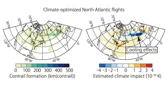
 [Green Version]
Figure 1. Daily mean geopotential height anomaly (red–blue contours) and zonal wind above 40 ms−1 (green contours with interval 5 ms−1) at 250 hPa for representative days in winter: (a) type W1 on 12 January, 2010; (b) type W2 on 1 January, 2015; (c) type W3 on 9 January, 2012; (d) type W4 on 20 December, 2009; and (e) type W5 on 19 February, 2012. “H” and “L” represent the high and low geopotential height anomalies.
Aerospace 08 00033 g001
Figure 2. Daily mean geopotential height anomaly (red–blue contours) and zonal wind above 20 ms−1 (green contours with an interval of 5 ms−1) at 250 hPa for representative days in summer: (a) type S1 on 11 July, 2009; (b) type S2 on 1 August, 2016; and (c) type S3 on 26 July, 2011. “H” and “L” represent high and low geopotential height anomalies.
Aerospace 08 00033 g002
Figure 3. Flight characteristics obtained from the one-day air traffic simulations for representative days of each weather type over the North Atlantic. The bars indicate the sum of 103 flights flying with different aircraft routing options. ATR20total is calculated by the algorithmic climate change functions (aCCFs) (see text for details).
Aerospace 08 00033 g003
Figure 4. Vertically integrated distribution of the climate impact (ATR20total) in winter (types W1 to W5) and in summer (types S1 to S3); those values are calculated by the aCCFs: (left) COC option; (center) contrail option; and (right) climate option. The distributions represent the sum of 103 flights for 24 h of the respective days. The arrows indicate the region where the climate impact changes significantly.
Aerospace 08 00033 g004
Figure 5. Relative changes in the flight time and fuel use for the one-day air traffic simulations with the time and the fuel routing options, including the enlarged drawing of the fuel optimal results. A symbol indicates the combined effect of 103 flights; for all the weather types, the results of the COC routing option are taken as the reference indicated by the cross “x” at the point of origin.
Aerospace 08 00033 g005
Figure 6. Changes in ATR20 components obtained from one-day air traffic simulations for the representative days of each weather type. For each type, three bars show the results for the COC, contrail and climate options. A bar consists of the values of ATR20 of ozone, methane, water vapor, CO2 and contrails; those values are calculated by the aCCFs. The individually colored components of the bar are stacked according to their positive or negative temperature responses.
Aerospace 08 00033 g006
Figure 7. Vertically integrated distribution of contrail distance for types W1, W4, S1 and S2: (left) COC option; (center) contrail option; (right) climate option. The distributions represent the sum of 103 flights for 24 h of the respective days. The arrows indicate the region where the contrail formation changes significantly.
Aerospace 08 00033 g007
Figure 8. Contrail distance vs. ATR20contrail for 103 individual flights obtained by the COC, the contrail and the climate options for the respective weather types.
Aerospace 08 00033 g008
Table 1. Setup for the European Center Hamburg general circulation model (ECHAM) and the Modular Earth Submodel System (MESSy) Atmospheric Chemistry (EMAC) model simulations.
ParameterDescription
ECHAM5 resolutionT42L90MA (2.8° by 2.8° in latitude and longitude, up to 0.01 hPa)
Simulation periodDecember 2008–August 2018 (ten years)
Time step length of EMAC12 min
EMAC mode of operationSpecified dynamics by nudging with ERA-Interim reanalysis dataset
Table 2. Setup for the air traffic simulations by the AirTraf submodel. “FL290” stands for a flight level at 29,000 ft. The setup of the second group (divided by rows) is used for Adaptive Range Multi-Objective Genetic Algorithm (ARMOGA) [39,40,41]. In ARMOGA, the Blend crossover operator (BLX(Blend crossover)-α; [43]) is employed with a user-specified crossover parameter α; the revised polynomial mutation operator [44] is employed with a mutation rate rm and with an external parameter controlling the shape of the probability distribution ηm. Details of these parameters are described by Yamashita et al. [27].
ParameterDescription
Flight plan103 North Atlantic flights (52 eastbound/51 westbound) [11,45]
Simulation periodOne day
Aircraft/engine typeA330-301/CF6-80E1A2, 2GE051 (with 1862M39 combustor)
Mach number0.82
Flight altitude change[FL290, FL410] (≈ [8.8, 12.5] km)
Number of waypoints101
Aircraft routing optionFlight time, fuel use, COC, contrail formation, climate impact
Coupled submodelsCONTRAIL, ACCF
Design variable11 (6 locations and 5 altitudes)
Population size100
Number of generations100
SelectionStochastic universal sampling
CrossoverBlend crossover BLX-α (α = 0.2)
MutationRevised polynomial mutation (rm = 0.1; ηm = 5.0)
Table 3. North Atlantic weather types for winter and summer. This classification refers to Table 1 of Irvine et al. [34]. In the second column, “+” stands for positive regimes of the North Atlantic Oscillation (NAO)/East Atlantic (EA) patterns, where anomaly fields have the same structure as typical NAO and EA teleconnection patterns; and “−” stands for their negative regimes, where anomaly fields have the same structure of the opposite sign.
TypeNAO/EA IndicesJet Stream Position/StrengthFrequency (Days/Season)Representative Day in 2008–2018
W1EA+Zonal/strong14.712 January 2010
W2NAO+Tilted/strong17.81 January 2015
W3EA−Tilted/weak18.99 January 2012
W4NAO−Confined/strong16.820 December 2009
W5MixedConfined/weak22.019 February 2012
S1EA+Zonal/strong26.011 July 2009
S2MixedWeakly tilted/weak43.11 August 2016
S3EA−Strongly tilted/weak22.926 July 2011
Publisher’s Note: MDPI stays neutral with regard to jurisdictional claims in published maps and institutional affiliations.

