Burn Time Correction of Start-Up Transients for CAMUI Type Hybrid Rocket Engine

Abstract

Burn time errors caused by various start-up transient effects have a significant influence on the regression modelling of hybrid rockets. Their influence is especially pronounced in the simulation model of the Cascaded Multi Impinging Jet (CAMUI) hybrid rocket engine. This paper analyses these transient burn time errors and their effect on the regression simulations for short burn time engines. To address these errors, the equivalent burn time is introduced and is defined as the time the engine would burn if it were burning at its steady-state level throughout the burn time to achieve the measured total impulse. The accuracy of the regression simulation with and without the use of equivalent burn time is then finally compared. Equivalent burn time is shown to address the burn time issue successfully for port regression and, therefore, also for other types of cylindrical port hybrid rocket engines. For the CAMUI-specific impinging jet fore-end and back-end surfaces, though, the results are inconclusive.

1. Introduction

In recent years, there has been an increasing trend of development of new rocket systems using hybrid rocket technology [1]. This trend is due to the essentially non-explosive nature of the hybrid propulsion rocket system. Hybrid rockets are inherently safer than their liquid or solid counterparts as the fuel and oxidizer are in separate states, in this case, solid state and liquid state. These separate states remove the possibility of uncontrolled mixing, and consequently, an explosion if any part of the engine ruptures [2]. This robustness against explosion is a strongly desirable trait, especially in the operation of very small, low-cost launchers, be they for suborbital or orbital flights. Once the cost of the launcher hardware is low enough, the ground costs become the main expense, with a substantial part of this being due to the explosive nature of conventional solid and liquid bi-propellant rocket engines [3]. Hybrid rockets avoid this cost but have traditionally had too low fuel regression rates and, therefore, too small thrust to weight ratios to be very useful as boosters.

1.1. CAMUI Hybrid Rocket Engine and Simulator

The Cascaded Multi-stage Impinging Jet (CAMUI) hybrid rocket engine solves this problem mentioned above of a low thrust to weight ratio. It is currently being developed as a powerful hybrid rocket engine with the potential of being used for sounding rockets, orbital booster stages, and satellite apogee kick engines. The principle of the CAMUI fuel geometry is shown below in Figure 1.

This geometry causes the hot combustion gasses to impinge multiple times on the fuel surfaces when exiting each port, thereby significantly increasing heat transfer to the fuel and, consequently, the fuel regression rate and overall engine thrust-to-weight ratio.

Test firings of up to 15 kN CAMUI engines with 15 s burn time have been performed successfully. At this size, though, and even more so at larger sizes, the cost of test firings starts to be prohibitive with the existing resources. It is, therefore, critical to have a good prediction model of the engine to minimize the necessary number of test firings needed to optimize a given engine class. For the simulation considered here, the burning of a fuel block is defined to happen differently on the three main burning surfaces: Fore-end surface, port, and back-end surface, as shown in Figure 1.

The existing model for fuel regression is based on Equations (1)–(4). These are derived from Nagata et al’s [4] adaptation of Marxman’s diffusion-limited model [5], and have been further adapted to include a scaling factor to account for the change in dimensions during burning:

$$\mathbf{Fore-end}\mathbf{surface}:r_{fu}=a_u(o/f)\ast G_p^{mu}{(\frac{H}{D_p})}^{nu}\ast {(\frac{D_p}{D_{pi}})}^{(mu-1)}$$

(1)

$$\mathbf{Port}:r_{fp}=a_p(o/f)\ast G_p^{mp}\ast {(\frac{D_p}{D_{pi}})}^{(mp-1)}$$

(2)

$$\mathbf{Back-end}\mathbf{surface}:r_{fd}=a_d(o/f)\ast G_p^{m}d\ast {(\frac{H}{H_i})}^{nd}\ast {(\frac{D_p}{D_{pi}})}^{(md-1)}$$

(3)

$$\mathbf{a-function}:a(o/f)=c1+c2\ast exp({(-\frac{ln(o/f)/c3}{c4})}^2)$$

(4)

Note that $a(o/f)$ is calculated separately for each of the 3 burning surfaces resulting in separate constants $c1,c2,c3$ and $c4$ for each of the a-functions $a_u(o/f),a_p(o/f)$ and $a_d(o/f)$.

As the port regressions are modelled as self-standing conventional (cylindrical) hybrid rocket, both the simulation methodology as well as the problems of it and their solutions are equally applicable to the regression simulation of any such conventional cylindrical hybrid rocket.

Note that, to measure the empirical regression rate, the fuel shape before and after firing is measured and the total regression is then divided by the burn time to get the regression rate. This method assumes a linear regression through time and the same linear regression is assumed when defining the fuel geometry for scaling. As the regression is non-linear [6,7], this may cause some additional error that is not addressed in this work.

Table 1. Nomenclatures used in this research.

a	function of $\mathit{O}/\mathit{F}$	H	Height (between fore- and back-end surfaces) (mm)	$\mathit{n}\mathit{u}$	Empirical constant (fore-end surface)
$D_p$	Port diameter (mm)	$H_i$	Initial height (mm)	$Re$	Reynolds number
$D_{pi}$	Initial port diameter (mm)	$md$	Empirical constant (back-end surface)	$R_{fd}$	Total regression back-end surface (mm)
F	Force of engine thrust (N)	$mp$	Empirical constant (port)	$R_{fp}$	Total regression port (mm)
$F_{steadystate}$	Force of engine thrust at steady state (N)	$mu$	Empirical constant (fore-end surface)	$R_{fu}$	Total regression fore-end surface (mm)
$G_p$	Propellant mass flux (kg/s/m${}^2$)	$nd$	Empirical constant (back-end surface)	$r_{fd}$	Regression rate back-end surface (mm)
$r_{fp}$	Regression rate port (mm)	$r_{fu}$	Regression rate fore-end surface (mm)	$tb$	Burn time (s)
$t{b}_{eq}$	Equivalent burn time (s)

shows the definition of the variables in the equations.

1.2. Problematic of Start-Up Transient

The current simulation model assumes a perfect burn with no start-up transient. As can be seen in the example of Figure 2, this is not the case as it takes a couple of seconds for the burn to reach its steady-state. As discussed in [8], this start-up transient is almost entirely caused by the slow build-up of stable oxidizer supply to the engine. Comparatively the ignition start-up where we have a build-up of temperature in the combustion area for the CAMUI engine is in the order of 0.1 s [8] and therefore negligible compared to the overall transient time. For this reason the diffusion limited model as described in Equations (1)–(4) is used exclusively in this work and other combustion mechanisms that happen during the much shorter ignition part of the transient time are not taken into account.

Compared to the typical CAMUI burn time of 2–10 s, a 2-s transient is a very significant time. Because the simulation model uses averaged values, this start-up transient will cause an error in the empirically derived constants used in the regression model. Note that the LOX flow measurement is unreliable for the first half-second or so [8]. Therefore, if using the measured LOX flow in the simulator, the LOX flow during this time is taken to be a linear rising LOX flow, from 0 at the beginning of chamber pressure/thrust rise to the measured LOX flow at what is deemed the LOX flow measurement stabilization point. After that, the simulated LOX flow is the measured LOX flow. In this case the simulated and actual measured LOX flow can be seen in Figure 2. As described in [8], using the existing model, based on Equations (1)–(3), to evaluate the resulting regression error for a ±30% burn time error, shows that the resulting regression error reaches up to 60% for a 30% burn time error. For these results, the 230 mm diameter high Reynolds number engine (230 Hi) were used for analysis. Figure 3 show that the burn time error has a disproportionately large effect on the regression accuracy. Here the “high tb” indicates simulation done where the analysed data has a 30% burn time added to the actual burn time as an artificial error to estimate the regression rate. Likewise, “low tb” indicates simulation done where the analysed data has a 30% burn time deducted from the actual burn time as an artificial error to estimate the regression rate. The regression is then simulated with the correct burn times. This causes two effects, firstly the changed burn time directly affects the estimated regression rate. The second effect is that the changed regression rate causes a erroneous shift in the assumed O/F ratio at the given regression rate. Combined, this gives a significant potential error in the simulated regression accuracy. This conclusion follows well the uncertainty analysis performed by Frederick et al. [9] on the effects of start-up transients for traditional tube-shaped hybrid rockets. However, where they measured start-up transient times of around 0.2 s compared to a 2 s burn time, the CAMUI, using liquid oxygen, has up to 2 s transient times for similar burn times so almost ten times larger. Despite their shorter transient times, they concluded that this effect was the most significant uncertainty effect on the regression rate estimation. A more recent analysis of the length of the start-up transient and the impact of the local oxidizer flow rate on the start-up transient time is presented by Cai et al. [10]. This analysis shows transient times varying from around 0.2 s to over 1-s fitting well with the engines used by both Frederick et al. [9] and Viscor et al. [8] as used in this research. This supports that for CAMUI, the transient effect is by far the most significant uncertainty for the regression estimation.

It is important to note that sufficiently long burn times will negate this error. Although to achieve as large a test firing database as currently exists (over 100 firings), this would necessitate re-doing a large number of tests for longer burn times. Furthermore, longer burn times mean larger and more expensive engines.

To allow for the efficient use of the existing test-firing data, we propose to adjust the simulation model to take this transient time phenomenon into account. This paper investigates the burn time errors associated with start-up transients. It introduces a method for overcoming these transients when applying test data to an empirical correlation of Marxman’s diffusion-limited regression model based on the analysis of recent CAMUI-type hybrid rocket test data.

This paper is organized as follows, Section 2 presents the implemented simulator and proposed method for overcoming these transients, Section 3 shows its results of the new model, Section 4 discusses its efficiency to minimize the overall simulation error, followed by an outlook of this work in Section 5.

2. Methodology

A comprehensive CAMUI simulator was developed in Matlab to help analyze the regression characteristics of the CAMUI engine for this research.

This simulator uses one set of engine tests to create a regression simulator for the prediction of other engine tests. The principle of the simulator is to import the test data from one series of engine test firings and then analyze this data to extract the empirical regression constants $m,c1,c2,c3$ and $c4$ for each of the 3 burning surfaces. These constants are then used in the regression simulator together with the regression formulas, Equations (1)–(4), to simulate the regression of any other CAMUI type engine. This simulator concept is illustrated in Figure 4. Based on this simulator, equivalent burn time is defined such that, when used in the constants analyzer part of the CAMUI simulator, it will give the corrected regression constants for the steady-state burning.

As illustrated in Figure 5, this equivalent burn time for each engine firing is found by first measuring the total impulse (in Newton seconds) of the given test firing and manually defining the steady-state thrust level $F_{steadystate}$. This $F_{steadystate}$ is found by looking at the thrust curve and visually evaluating when the start-up transient has ended, and thereby the steady-state level has been reached. The equivalent burn time is then the time the engine would be firing at this steady-state thrust level to achieve the measured total impulse. Mathematically, this is done as shown in Equation (5).

$$t_{b_{eq}}=\frac{\int Fdt}{F_{steadystate}}$$

(5)

This equivalent burn time is then implemented into the constants analyzer, resulting in adjusted $a(o/f)$ functions and m values in Equations (1)–(3), closer to the actual steady-state values rather than the time-averaged values. This then results in overall higher simulated regression rates and resulting thrust.

To conceptualize the change in burn time error when using these equivalent burn time derived constants versus the nominal burn time derived constants in the regression simulator, the errors for the two cases have been illustrated in Figure 6. Note that, for better visualization, the simulations here are illustrated with the assumption of an instantaneous steady-state LOX flow. Figure 6 shows, conceptually, the results from simulated versus actual performance when using nominal (top) and equivalent burn time (bottom)for the derivation of the regression constants in the analysis part of the simulator. In Figure 6 (top), we see the expected error from the simulation with nominal burn time derived constants split into two regions, namely the overshoot region where the regression rate is overestimated and the undershoot region where the regression rate is underestimated.

In the case of simulating an engine that is similar to the engines used for derivation of the constants in the constants analyser, the nominal burn time overshoot error and undershoot error cancel out each other in the averaging analysis. Using burn time equivalent, in this case, will only increase the overshoot error and additionally remove the balancing undershoot error, causing an overall increased error in the simulated engine. However, when the simulated engine has a longer burn time than the analysed engines used for the derivation of the constants, then the undershoot error grows proportionally to the burn time while the overshoot error stays the same, creating an increasing overall error in the simulated engine. Once this error growth becomes larger than the additional burn time equivalent overshoot error, it should theoretically be advantageous to use equivalent burn time. Similarly, if the simulated engine has a shorter transient time than the analysis engines, the overshoot error is reduced while the undershoot error stays the same. Once this reduction in overshoot error is larger than the initial undershoot error, it again is expected to become advantageous to use equivalent burn time.

To investigate this empirically, the results from regression simulations with and without the use of equivalent burn time are compared to the results from a number of firing tests. The measured LOX flows from the firing tests are used as oxidizer inputs for these simulations. This reduces to some degree the overshoot error, but does not eliminate it as other transient effects are still unresolved. The engine test series used in this analysis are shown below in

Table 2. Engines used in this research.

Engine Name	Number of Fuel Blocks per Engine	Fuel Outer Diameter (mm)	Nominal Thrust Level (kN)	Burn Times (s)	Burn Time Category	Re Number ·${10}^4$
100 Lo	10	100	2.5	2–5	short	1–5
230 Hi	10	230	10	5–10	medium	10–20
200 Lo	7	200	2	5–25	long	1–5
200 Hi	8	200	4	5–10	medium	10–20

.

Following Nagata et al. [11], the engines in this research are grouped into two categories, namely high Reynolds number engines and low Reynolds number engines. The 100 Lo engines are similar in Re number to the 200 Lo engines, while the 230 Hi engines are similar to the 200 Hi engines. Therefore, 100 Lo results are used in the constants analyzer for the simulation of both the 100 Lo engines as well as the 200 Lo engines. Similarly, the 230 Hi engines are used in the constants analyzer for the simulation of both the 230 Hi engine and the 200 Hi engines.

Figure 7 shows the overall calculation flow when using nominal burn time (left), and when using equivalent burn time (right).

Using just nominal burn time as shown in Figure 7 (left), the empirical regression constants $m,c1,c2,c3$ and $c4$ are found for each of the 3 burning surfaces. This is based on the data from all engines in a single test series (either 100 Lo or 230 Hi). These constants are then used to simulate the regression of each surface on each fuel block for each individual engine in a test series (100 Lo, 200 Lo, 230 Hi and 200 Hi). Lastly these individual surface total regression rates are compared with the measured ones. in the case of using equivalent burn time as shown in Figure 7 (right), before extract the regression constants, the equivalent burn times for each engine firing in the series is calculated according to Equation (5). These equivalent burn times ($t{b}_{eq}$) are then used instead of the nominal burn times when extracting the empirical constants $m,c1,c2,c3$ and $c4$ for each of the 3 burning surfaces. The regression of each surface on each fuel block for each individual engine in a test series (100 Lo, 200 Lo, 230 Hi and 200 Hi) is then simulated using the nominal burn time $tb$. Lastly these individual surface total regression rates are compared with the measured ones.

3. Results

Using the described method of finding $t{b}_{eq}$ the resulting change in burn time is described below in

Table 3. $tb$ vs. $t{b}_{eq}$ for 100 Lo.

Engine Number	1	2	3	4	5	6	7
$tb$	5.3	4.2	2.2	2.2	2.3	3	3.2
$t{b}_{eq}$	4.7	3.5	2	2.1	2	2.6	2.6
% $tb$ reduction	11%	17%	10%	5%	13%	13%	19%

for the 100 Lo test series and in

Table 4. $tb$ vs. $t{b}_{eq}$ for 230 Hi.

Engine Number	1	2	3	4	5	6
$tb$	10.2	5.5	6.9	5.3	4.8	5
$t{b}_{eq}$	10	5.1	6	4.9	4.3	4.4
% $tb$ reduction	2%	7%	13%	8%	10%	12%

for the 230 Hi test series.

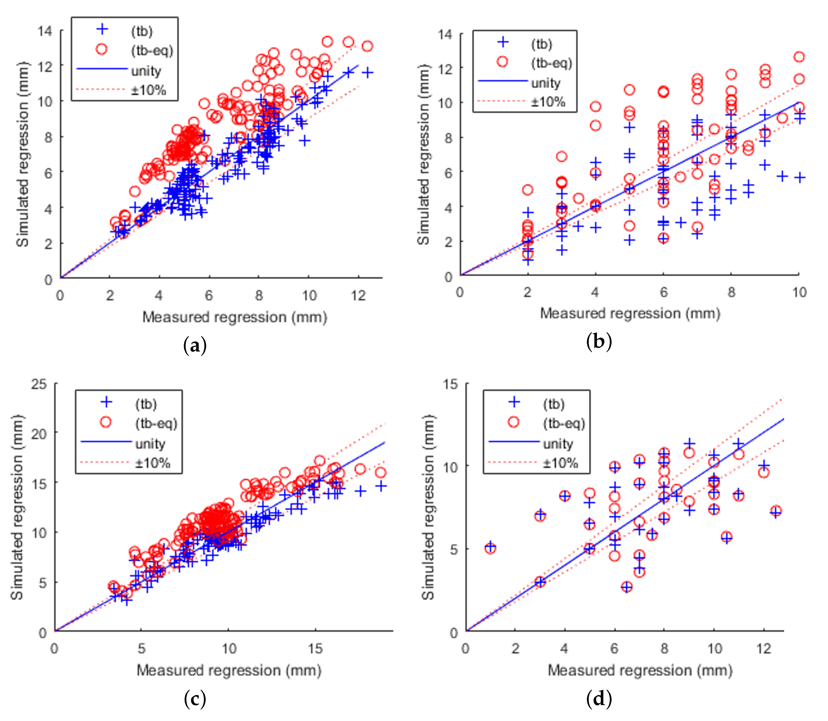
When focusing on the port surface regressions, the simulation results become as shown in Figure 8a for the analysis of 100 Lo data to simulate 100 Lo firing, Figure 8b for analysis of 100 Lo data to simulate 200 Lo firing, Figure 8c for analysis of 230 Hi data for 230 Hi simulation, and Figure 8d for analysis of 230 Hi data to simulate 200 Hi firing. Calculating the port regression error RMS for simulated vs. measured regression for the same analysis and test firing scenarios with and without the use of the burn time equivalent, we get results as shown in

Table 5. Simulated port regression error (RMS).

Analysis Baseline Engine	100 Lo		230 Hi
Simulated engine	100 Lo	200 Lo	230 Hi	200 Hi
Simulated engine	100 Lo	200 Lo	230 Hi	200 Hi
Error RMS $tb$	15%	41%	14%	27%
Error RMS $t{b}_{eq}$	47%	18%	24%	24%

.

We then look at the results for all burning surfaces. Figure 9a,b shows, respectively, the 100 Lo and 200 Lo results when using the 100 Lo data for analysis with and without $t{b}_{eq}$. Likewise, using the 230 Hi data for analysis with and without $t{b}_{eq}$ gives the 230 Hi results, as shown in Figure 9c and the 200 Hi results shown in Figure 9d.

4. Discussion

Considering the port regression, when using the 100 Lo series both as the analysis baseline as well as the simulate test case, using the nominal burn time gives a very accurate simulation. This is shown in Figure 8a, and results in an error RMS of 15% while using the equivalent burn time considerably increases the error to an RMS of 41%. The same pattern can be seen in Figure 8c with an increase of error RMS from 14% for nominal burn time to 24% for equivalent burn time. These results are as expected as the analysis engines are the same (averaged) as the simulated engines where using nominal burn time should give the best results. That the effect is considerably more significant for the 100 Lo series in Figure 8a than for the 230 Hi series in Figure 8c is caused by the relatively larger difference between the start-up transient length and burn time with the 100 Lo series having similar start-up transient times but much shorter overall burn times compared to the 230 Hi series. This results in a larger percentual change of burn time for the 100 Lo engines compared to the 230 Hi engines. The effects of introducing the equivalent burn time are, therefore, more significant.

In Figure 8b the 100 Lo series was used in the constants analyzer to simulate the 200 Lo series. Here we see that the use of equivalent burn time has a substantial positive effect on the simulation accuracy. The use of equivalent burn time reduces the simulated regression error RMS from 41% with nominal burn time to 18 %. This result also follows expectations in that the 100 Lo test series, which is used for the analysis, has long start-up transients and very short burn times. The use of equivalent burn time correctly predicts how the regression would be when this burn time is extended in the long-burning 200 Lo series, which furthermore has shorter transient times as well. A similar trend is seen in Figure 8d with the use of 230 Hi series for analysis and 200 Hi for the firing simulation comparison. The error RMS, in this case, is reduced from 27% to 24%. The effect here, though, is much smaller. This again fits the expected results, as the 230 Hi burn times are more similar to the 200 Hi burn times than those of 200 Lo are to 100 Lo. When looking at the results for all the burn surfaces, for Figure 9a,c, the simulation using equivalent burn time performs worse than the nominal as expected like in the port only case. For Figure 9b,d though, it is not clear that using the equivalent burn time is an improvement over nominal burn time. As mentioned in [8], other uncertainties have a significant effect on the regression simulator for the upstream and downstream surfaces. It is believed that we are here running into the problem that the overall regression modelling accuracy for the fore- and back-end surfaces is inadequate to evaluate the effect of the equivalent burn time.

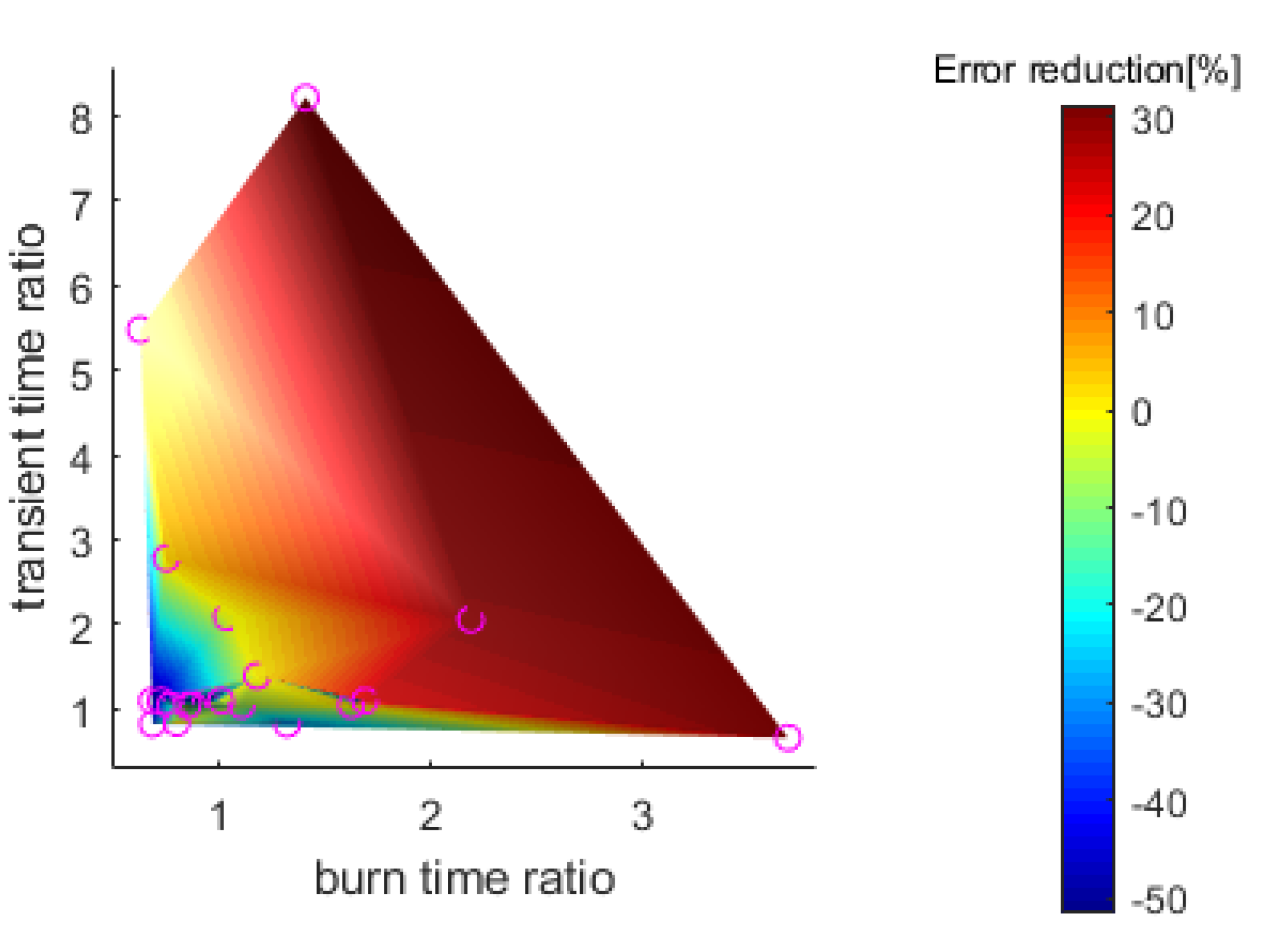
The above discussion shows that equivalent burn time can improve the error in regression modelling caused by start-up transients under certain conditions, namely when the simulated engine has a longer burn time and or shorter transient time than the engines used for the analysis. To concretize “longer” and “shorter” the effect on error RMS of each engine has been plotted in Figure 10. For better visualization, the value points have been interpolated to create a 3D surface. The data points from each individual engine are shown (pink circle) with:

• Error reduction (delta error RMS) = error RMS ($tb$) – error RMS($t{b}_{eq}$);
• Burnt time ratio = $tb$ (simulated)/$tb$ (analysed);
• Transient time ratio = $tt$ (analysed)/$tt$ (simulated).

The times, $tt$ (analysed) and $tb$ (analysed), are the ratio between the averaged transient times of all the engines in the analysis test series and the transient time of the given simulated engine. The simulated times are for each individual engine.

Figure 10 illustrates that with increasing simulated burn time and decreasing simulated transient time compared to the analysed values, an increasing error reduction is achieved by using the equivalent burn time. Figure 11 is a top view of the same graph shown in Figure 10. This view allows us to clearly see the demarcation line (yellow area) that shows the border between when it is an advantage to use equivalent burn time (above of the yellow 0-value line), and when it is a disadvantage (below the yellow line).

Based on this, it is therefore believed by the authors that the use of equivalent burn time is valid for the described cases where the simulated engines have longer burn time or shorter transient times, as shown in Figure 10 and Figure 11. With the existing regression model, this can currently only be validated for the port regression as other errors overshadow the effects of the equivalent burn time for the end face regression simulations. The validation of the use for the port regression modeling, though, also shows that this method is valid for use on all conventional cylindrical hybrid rocket engines.

5. Conclusions

To address the problem of start-up transients’ effect on burn time definition, and therefore regression simulation, the equivalent burn time has been defined. Though inconclusive for the end face regression surfaces, for port regression, and therefore also for other types of cylindrical port hybrid rocket fuels, the equivalent burn time methodology has shown to be a useful tool to reduce errors caused when short burn time engines with relatively large start-up transients are used as a baseline to simulate the performance of longer burn time engines or shorter transient time engines. Equivalent burn time is, therefore, now an integral part of the overall CAMUI simulator and is being used for future engine designs.