Article

Sensitivity-Based Non-Linear Model Predictive Control for Aircraft Descent Operations Subject to Time Constraints

1
Department of Physics, Technical University of Catalonia (UPC), 08860 Castelldefels, Spain
2
Crew Systems and Aviation Operations Branch, NASA Langley Research Center (LaRC), Hampton, VA 23666, USA
*
Author to whom correspondence should be addressed.
Aerospace 2021, 8(12), 377; https://doi.org/10.3390/aerospace8120377
Submission received: 3 November 2021 / Revised: 30 November 2021 / Accepted: 2 December 2021 / Published: 4 December 2021

Abstract

:
The ability to meet a controlled time of arrival while also flying a continuous descent operation will enable environmentally friendly and fuel efficient descent operations while simultaneously maintaining airport throughput. Previous work showed that model predictive control, a guidance strategy based on a reiterated update of the optimal trajectory during the descent, provides excellent environmental impact mitigation figures while meeting operational constraints in the presence of modeling errors. Despite that, the computational delay associated with the solution of the trajectory optimization problem could lead to performance degradation and stability issues. This paper proposes two guidance strategies based on the theory of neighboring extremals that alleviate this problem. Parametric sensitivities are obtained by linearization of the necessary conditions of optimality along the active optimal trajectory plan to rapidly update it for small perturbations, effectively converting the complex and time consuming non-linear programming problem into a manageable quadratic programming problem. Promising results, derived from more than 4000 simulations, show that the performance of this method is comparable to that of instantaneously recalculating the optimal trajectory at each time sample.

1. Introduction

Continuous descent operations (CDOs) with controlled times of arrival (CTAs) at one or several metering or merging fixes could enable more environmentally friendly procedures without compromising airspace or airport throughput. This type of flight operation requires flight management systems (FMSs) not only able to compute (i.e., plan) an optimal trajectory satisfying CTAs, but also to safely and efficiently guide the aircraft during the execution of the descent, such that these time constraints are successfully satisfied by the actual flown trajectory.
The computation of the optimal trajectory plan can be formulated as an optimal control problem [1], in which a given cost function (e.g., fuel consumption) is to be minimized while satisfying a set of constraints, including the CTA(s). Typical FMSs compute the optimal trajectory plan before starting the descent. Then, the trajectory plan is “frozen” and the guidance system executes it. This initial trajectory plan, however, only shows what can be achieved given a perfect (deterministic) knowledge of the model of the whole system (driven by models on aircraft dynamics and weather). When the models used by the trajectory planning function of the FMS do not match the reality, the initial trajectory plan is no longer optimal and some operational constraints (including CTAs) may even be violated if errors are not actively nullified by the guidance system.
In recent years, an interesting research effort has been devoted to taking into account system uncertainties and to derive methodologies for robust or stochastic aircraft trajectory planning. See, for instance [2], where weather uncertainty is considered by means of probabilistic forecasts generated by ensemble prediction systems and a robust trajectory plan is obtained in such a way that the same track and true airspeed are followed in all possible weather scenarios (weather ensembles), and the expected value of a given cost function is minimized. A similar approach was recently presented in [3], particularly addressing the robust optimization of CDOs with a CTA. Since true airspeed is fixed in all (different) weather ensembles, the ground speed is different in each particular ensemble and, therefore, the fulfillment of the CTA cannot be ensured. Instead, the proposed algorithm minimizes the expected value of the CTA time error at the metering/merging fix. Although these robust strategies might certainly help to reduce uncertainty in the trajectory planning function of the FMS, an efficient guidance function is still needed in order to achieve CTAs in the executed trajectories with high levels of accuracy, while trying to minimize the differences of the flown trajectory with respect to the initially planed one, especially in certain variables such as fuel consumption or the energy deviation at the metering/merging fix.
In our previous work [4], the performance of various guidance strategies in the time and energy managed operations concept [5] were compared using a high-fidelity fast-time flight simulator, focusing on the environmental impact mitigation and the ability to meet operational constraints. Numerous descents subject to CTAs were simulated, with errors introduced in the parameters of the weather and aircraft performance models used by the trajectory planning function of the FMS. Results showed that the non-linear model predictive control (NMPC) [6], a guidance strategy based on a frequent update of the optimal trajectory plan during the execution of the descent, is very robust in terms of correcting energy (speed and altitude) and time deviations, providing at the same time acceptable fuel consumption and noise figures. NMPC was also compared to "typical" guidance strategies (similar to those implemented by most FMSs) in [7], demonstrating superior performance in terms of CTA compliance and fuel efficiency. Other relevant applications of model predictive control in the aviation field can be found in [8,9,10].
Typical NMPC strategies update the optimal trajectory plan by solving a non-linear programming (NLP) optimization problem, referred to in this paper as ideal NMPC (INMPC) [11]. Ideally, the NLP optimization problem is solved instantaneously right after measuring the actual state of the aircraft. In practical applications, however, solving the NLP optimization problem may take a significant amount of time, leading to stability issues and/or degrading the performance of the operation [11]. In order to reduce the execution time, educated simplifications in the models used by the trajectory planning function of the FMS could be used [12], at the expense of compromising the accuracy of the resulting trajectory plan. Other NMPC implementations compensate for computational delay by starting the optimization in advance, setting the initial conditions of the new trajectory plan to the predicted state of the aircraft at the next time sample [13], or at a look-ahead time equal to the estimated execution time. In the latter case, the unpredictability of the execution time remains a critical issue [14].
An alternative method widely used in process industries, such as chemical manufacturing and oil refineries, consists of computing fast trajectory updates in the neighborhood of the active optimal trajectory plan using the theory of neighboring extremals [15]. Parametric sensitivities are obtained by linearization of the necessary conditions of optimality along the active optimal trajectory plan to rapidly update it for small perturbations in the (uncertain) parameters of the model. This strategy, known as sensitivity-based NMPC (SbNMPC), has shown an important reduction of execution time [16,17,18].
In previous work [19], the SbNMPC strategy was implemented to guide aircraft during CDOs subject to CTAs, and 15 representative descents were simulated introducing errors in the parameters used by the FMS to describe the wind profile. Then, the performance of SbNMPC in terms of fuel consumption and ability to satisfy operational constraints was compared with those of the open-loop execution and the INMPC. This paper extends the experiment to more than 4000 descents per guidance strategy in order to draw conclusions based on statistically meaningful results. Another contribution of this paper is to assess the performance of an alternative guidance strategy, referred to as Advanced step NMPC (AsNMPC), which combines an early recalculation of the trajectory plan based on the predicted state at the next time sample with a sensitivity-based update to correct perturbations right after measuring the actual state. The sensitivity of the performance metrics to the mean longitudinal wind error experienced during the execution of the descent is also investigated for the three different guidance strategies compared to the performance of the open-loop descent execution. Last but not least, this paper proposes a generic formulation of the trajectory optimization problem using direct methods, which goes beyond the descent phase.

2. Trajectory Management Using NMPC

NMPC was introduced to the process industry in the 1970s. This guidance strategy is based on the solution, at each time sample, of an optimal control problem over a future time horizon [6]. The resulting optimal control is applied only until the next time sample, when the optimal control problem is solved again, and so on. Typical NMPC applications consider a fixed-length time horizon, which advances an interval sample at each recalculation. When the system has to reach a certain state in a fixed amount of time (as in this paper), a shrinking horizon is often preferred. Using this strategy, the length of the horizon decreases by one interval sample at each recalculation.
Section 2.1 formulates the multi-phase optimal control problem for the shrinking horizon NMPC, and shows how to solve the resulting parametric optimization problem. Depending on the algorithm used to update the optimal solution at each time sample, different NMPC variants can be defined. Section 2.2 presents the working principle of three NMPC guidance strategies investigated in this paper.

2.1. Trajectory Planning

Section 2.1.1 presents the generic optimal control problem formulation in the continuous domain over a shrinking horizon. Then, Section 2.1.2 presents a method to discretize the problem with direct methods. Finally, Section 2.1.3 describes a numerical approach to solve it by using non-linear programming (NLP) optimization solvers.

2.1.1. Optimal Control Problem Formulation in the Continuous Domain

An optimal control problem over a fixed or variable continuous time horizon t I , t F can be formulated as follows [1]:
min u ( t ) J : = ϕ x ( t F ) , d + t I t F π x ( t ) , u ( t ) , d d t s . t x ( t I ) = X x ˙ = f x ( t ) , u ( t ) , d , t [ t I , t F ] b i n x ( t ) , u ( t ) , d 0 , t [ t I , t F ] b e q x ( t ) , u ( t ) , d = 0 , t [ t I , t F ] ψ x ( t F ) , d = 0 ,
where x ( t ) n x is the vector of differential states; u ( t ) n u is the vector of controls; and d n d is the vector of fixed parameters of the model. The cost function J : n x × n u × n d , which is composed by a running cost (or Lagrange term) π : n x × n u × n d and an end cost (or Mayer term) ϕ : n x × n d , is to be minimized subject to: dynamic constraints f : n x × n u × n d n x in the form of ordinary differential equations (ODEs) with initial conditions X n x ; algebraic constraints b e q : n x × n u × n d n φ ; inequality path constraints b i n : n x × n u × n d n b ; and terminal constraints ψ : n x × n d n ψ .
In some applications, free parameters that, in contrast to the controls, are constant in time might be also included as a part of the decision variables. For instance, when the final time is fixed, t F is a known parameter; for optimal control problems with variable final time, however, t F becomes a new decision variable to be optimized, in addition to u ( t ) . Conversely, the vector of fixed parameters of the model, d, is not part of the decision variables (e.g., the CTA or the wind forecast) and, consequently, must be specified beforehand and remains constant during the whole optimization process.
Essentially, two different methods are available for solving Equation (1): indirect methods, which involve the calculus of variations or the maximum principle of Pontryagin [1]; and direct methods, which transform the original infinite-dimensional optimal control problem into a finite-dimensional NLP optimization problem [20]. On the one hand, the solution of optimal control problems with indirect methods requires the solution of a multi-point boundary value problem using an appropriate, multi-dimensional zero finding algorithm. The major drawback of these methods is the requirement for a detailed mathematical analysis of each single problem. Even slight changes in the constraints can lead to a completely different solution structure, often requiring a complete revision of any previous derivation of the necessary equations. On the other hand, direct methods parametrize the time histories of the control and possibly state variables at a set of time samples. The cost function and constraints of the optimal control problem can be expressed in terms of these parametrized controls and possibly states, which become the decision variables of a parametric NLP optimization problem.

2.1.2. Optimal Control Problem Discretization Using Direct Methods

Let the continuous time horizon t I , t F be discretized into N + 1 equidistant time samples τ k , with k = 0 , , N . Note that τ 0 = t I , τ N = t F and the discretization step is Δ τ = τ N τ 0 N (i.e., a time step is the difference between two consecutive time samples). The discrete optimal control problem minimizing the cost function J in a time horizon of N time intervals can be formulated as:
min x k , k = 0 , , N u k , k = 0 , , N 1 J : = ϕ x N , d + k = 0 N 1 Π x k , u k , d , Δ τ s . t x 0 = X x k + 1 = F x k , u k , d , Δ τ ; k = 0 , , N 1 b i n x k , u k , d 0 ; k = 0 , , N 1 b e q x k , u k , d = 0 ; k = 0 , , N 1 ψ x N , d = 0 ,
where x k n x and u k n u are the state and control vectors discretized at τ k , respectively, for k = 0 , , N . While the algebraic, path and terminal constraints of the continuous optimal control problem (1) can be directly evaluated at the discretized states and controls, the states evolution function F : n x × n u × n d × n x must be defined as the result of integrating f during a time interval of duration Δ τ using the discretized states and controls. Similarly, Π : n x × n u × n d × is a quadrature function resulting from a numerical integration of π during a time interval Δ τ .
The optimal control problem described by Equation (2) assumes that the same running cost, dynamic constraints and algebraic and path constraints apply during the whole time horizon. In addition, event constraints can be set only at the very end of the time horizon. Yet, many real-life processes can be divided into several phases, where the dynamics of the system, the cost and the constraints might change. In addition, in some applications it is necessary to formulate interior-point constraints in between two consecutive phases. Equation (2) can be extended to multi-phase problems.
First, let the continuous time horizon [ t I , t F ] be divided into P time intervals [ t j , t j + 1 ] for j = 0 , , P 1 ; each time interval corresponding to a different phase. Again, t 0 = t I and t P = t F . Then, each phase is discretized into N j equidistant time samples τ k , τ k + 1 , , τ k + N j 1 , where τ k = t j , τ k + N j 1 = t j + 1 and k = i < j N i , for all j = 0 , , P 1 . The discretization step of the jth phase is denoted by Δ τ j . As a result, the whole time horizon is discretized into N + 1 = j = 0 P 1 N j time samples τ 0 , τ 1 , , τ N .
Let T be a multi-dimensional set that relates the index of each phase to the indexes of its corresponding time samples. The subset E T only includes the index corresponding to the last time sample of each phase; and I is defined as T \ E . Based on the definitions stated above, the discrete multi-phase optimal control problem can be formulated as:
min x k , k = 0 , , N u k , ( j , k ) I J : = ( j , k ) E ϕ j x k , d + ( j , k ) I Π j x k , u k , d , Δ τ j s . t x 0 = X x k + 1 = F j x k , u k , d , Δ τ j ; ( j , k ) I b j i n x k , u k , d 0 ; ( j , k ) I b j e q x k , u k , d = 0 ; ( j , k ) I ϑ j e q x k , d = 0 ; ( j , k ) E \ { ( P 1 , N ) } ϑ j i n x k , d 0 ; ( j , k ) E \ { ( P 1 , N ) } ψ x N , d = 0 x k x k + 1 = 0 ; ( j , k ) E \ { ( P 1 , N ) } .
In Equation (3), Π j : n x × n u × n d × and F j : n x × n u × n d × n x are the quadrature and states evolution functions for the jth phase, respectively. Similarly, b j e q : n x × n u × n d n φ j and b j i n : n x × n u × n d n b j are the algebraic and path constraints, respectively, of the jth phase; and ϑ j e q : n x × n d n ϑ j e q , and ϑ j i n : n x × n d n ϑ j i n represent applicable equality and inequality interior-point constraints, respectively, applying at the last time of the jth phase. Note that, in the very last row of Equation (3), a new set of constraints has been added to link the state variables across two consecutive phases and guarantee continuity in the solution. For more details on this formulation, the reader could refer to [21].
Analogously to the single-phase optimal control problem, the discretization step of each individual phase could be considered either a known parameter or a variable to be optimized. For instance, if the duration of the whole time horizon were fixed to a certain parameter, say a CTA, but the duration of each phase was flexible, Δ τ j for j = 0 , , P 1 would become decision variables subject to the following constraint:
j = 0 P 1 N j 1 Δ τ j CTA = 0 ,
which would be appended to Equation (3).

2.1.3. Solution of the Direct Optimal Control Problem Using NLP Algorithms

As mentioned above, direct methods for optimal control compute the optimal trajectory plan by formulating the generic optimal control problem Equation (3) as a parametric NLP optimization problem of the form:
min z f z , p s . t h z , p = 0 g z , p 0 ,
where z n z is the vector of primal variables; h : n z × n p n h is the vector of equality constraints; g : n z × n p n g is the vector of inequality constraints; and p n p is the vector of (fixed) parameters of the NLP optimization problem. In this paper, the following definitions have been considered:
z : = z 0 z 1 z N , h z , p : = h 0 z , p h 1 z , p h N z , p , g z , p : = g 0 z , p g 1 z , p g N z , p ,
where
z k : = u k x k if ( j , k ) I x k if ( j , k ) E h k : = x k + 1 F j x k , u k , d , Δ τ j b j e q x k , u k , d if ( j , k ) I ϑ j e q x k , d x k x k + 1 if ( j , k ) E \ { ( P 1 , N ) } ψ x k , d if k = N g k : = b j i n x k , u k , d if ( j , k ) I ϑ j i n x k , d if ( j , k ) E \ { ( P 1 , N ) } .
Note that z k includes both discretized states and controls at τ k . Similarly, g k and h k include the inequality and equality constraints applied at τ k , respectively.
In Equation (5), f is the cost function of the original optimal control problem evaluated at the primal variables and NLP parameters, that is, f z , p = J ( z , p ) . In this paper, the vector of fixed NLP parameters is composed of both the current state of the aircraft and the fixed parameters of the model:
p = X , d T .
The Lagrangian function associated to the NLP optimization problem Equation (5) is:
L z , p , λ , μ : = f z , p + λ T g z , p + μ T h z , p ,
where λ n g and μ n h are the Lagrange multipliers (dual variables) vectors paired up with the constraints g and h, respectively. An optimal primal-dual pair z * , λ * , μ * satisfies the first-order necessary conditions of optimality, also known as Karush–Kuhn–Tucker (KKT) conditions if:
L z z * , p , λ * , μ * = 0
      h z * , p = 0
      g z * , p 0
      λ * T g z * , p = 0
         λ * 0 .
The inequality constraints in the optimal solution can be divided into two complementary sets: the active set ( G a c ) and the inactive set ( G i n ) [17]. All inequality constraints in the active set satisfy g z * , p = 0 . In the above notation, ( · ) * indicates optimal.
Let P N be the NLP algorithm (either interior-point or active-set) that provides the optimal primal-dual solution (i.e., satisfying Equation (10)) as a function of p for the next N time intervals:
z * , λ * , μ * P N p .
Remember that the vector of NLP parameters includes both current states and fixed parameters of the model (see Equation (8)). In addition, by definition of Equation (11), the optimal primal-dual solution of the NLP optimization problem is an implicit function of p. Therefore, any change in p would lead to a new optimal primal-dual solution.
Imagine a hypothetical case in which, at τ 0 , the algorithm P N has provided the optimal primal-dual solution in the time horizon τ 0 , τ 1 , , τ N . After implementing the optimal control u 0 * during the first time interval Δ τ , the system would be driven to a new state. Note that if the dynamic model and associated parameters d were perfect, the new state would correspond to F X , u 0 * , d , Δ τ . Assuming a situation in which the optimal primal-dual solution starting at the new state needs to be updated, the structure of the NLP optimization problem and the old primal-dual solution corresponding to the new time horizon τ 1 , , τ N could be used to speed up the optimization process. Stated in a more general form, the solution of the NLP optimization problem at any τ i , i = 1 , , N 1 could take advantage of the NLP optimization problem structure and the optimal primal-dual solution at any of the preceding time samples.
Firstly, the decision variables and constraints will be:
z i : : = z i z i + 1 z N , h i : z i , p : = h i z i , p h i + 1 z i : , p h N z i : , p , g i : z i : , p : = g i z i : , p g i + 1 z i : , p g N z i : , p ,
where · i : indicates the elements of · corresponding to time samples from τ i to the end of the time horizon ( τ N ).
The Lagrangian function of the NLP optimization problem starting at τ i is:
L i : z i : , p , λ i : , μ i : : = f i : z i : , p + λ i : T g i : z i : , p + μ i : T h i : z i : , p ,
and the KKT conditions Equation (10) also need to be satisfied at z i : * , λ i : * , μ i : * .
Let P N i be the NLP algorithm that provides the optimal primal-dual solution as a function of p, starting at τ i and for the next N i time intervals:
z i : * , λ i : * , μ i : * P N i p .
Secondly, NLP solvers are always executed from a starting point with all the primal and dual variables of the problem (unknowns of the problem) initialized to some value. Typically, the user can specify these starting values and, otherwise, the solver will just set all the unknowns to zero or to another random value. Then, from this starting point, the internal algorithm of the NLP solver aims to find a feasible (i.e., that fulfills all the constraints) and optimal (i.e., that either minimizes or maximizes the cost functional) solution. An appropriate starting point or initial estimate dramatically reduces the convergence time of the optimization, a key aspect when the problem is very complex. It should be noted that, since NLP solvers cannot guarantee a global optimum in non-convex problems, different initial estimate could lead to different sub-optimal solutions. When solving a sequence of related problems, the solution from the preceding optimization within the current time horizon should be used as an estimate. This technique, which typically reduces the execution time, is commonly known as warm start.

2.2. Trajectory Guidance

Depending on whether the optimal solution is updated at each time sample by solving a rigorous NLP optimization problem and/or by taking advantage of parametric sensitivities, the following NMPC guidance strategies can be defined:

2.2.1. Ideal NMPC (INMPC) Guidance

In an ideal case, problem P N i is solved at each time sample τ i , as soon as the parameter vector p is measured or estimated. Then, the resulting optimal control u i * is applied without delay until τ i + 1 , where the process is repeated. However, for achieving optimal performance and good stability properties, problem P N i needs to be solved instantaneously. We refer to this hypothetical case as the ideal NMPC (INMPC). Algorithm 1 details its main steps.
Algorithm 1 Working principle of the ideal NMPC (INMPC)
1:
z * , λ * , μ * P N p
2:
Build z 1 : * , λ 1 : * and μ 1 : * from z * , λ * and μ *
3:
for  i = 1 , , N 1 do
4:
    Measure X and estimate d
5:
     p X d
6:
     z i : * , λ i : * , μ i : * P N i p using warm start
7:
    Build z i + 1 : * , λ i + 1 : * and μ i + 1 : * from z i : * , λ i : * and μ i : *
8:
    Implement u i * until τ i + 1 .
Unfortunately, in practical applications,  P N i may be computationally expensive to solve. This implies that the control u i * cannot be applied just after p is measured or estimated, but only after  P N i is solved. The delay in calculating the new solution may lead to sub-optimum trajectories, failure to meet constraints, or in some instances instabilities of the solution [22]. This motivates the introduction of sensitivity-based methods to (approximately) update the optimal trajectory plan quasi instantaneously.

2.2.2. Sensitivity-Based NMPC (SbNMPC) Guidance

If the change in the parameters vector from one time sample to the next is small, parametric sensitivities at the active optimal solution can be used to rapidly update the optimal trajectory for any perturbation Δ p . The parametric sensitivities of the primal and dual variables with respect to the parameters vector at τ i , i = 0 , , N 1 can be obtained by differentiating the KKT conditions Equation (10) evaluated at the active optimal primal-dual solution:
z i : p λ i : p μ i : p = 2 L i : * z i : 2 g i : * z i : T h i : * z i : T g i : * z i : 0 0 h i : * z i : 0 0 1 2 L i : * z i : p g i : * p h i : * p .
Being consistent with the notation, ( · ) i : * = ( · ) ( z i : * , λ i : * , μ i : * , p ) . It is very important to remark that only active inequality constraints (i.e., those included in G a c , thus satisfying g z * , p = 0 ) can be considered in the linear system defined by Equation (15).
This linear system can be solved for z i : p , λ i : p and μ i : p , allowing us to update the optimal solution using a simple first-order Taylor approximation as follows:
z i : * ( p + Δ p ) = z i : * ( p ) + z i : p Δ p
λ i : * ( p + Δ p ) = λ i : * ( p ) + λ i : p Δ p
μ i : * ( p + Δ p ) = μ i : * ( p ) + μ i : p Δ p .
Unfortunately, this fast and convenient parametric sensitivity update can only be used if the set of active constraints does not change after the perturbation [17]. In practical NMPC applications, however, constraints in the active set may become inactive, or constraints in the inactive set may become active for the solution corresponding to the perturbed p. In this case, the approximate solution may no longer be accurate enough.
An interesting approach that accounts for active set changes after a perturbation in the NLP parameters vector was suggested by [23]. This approach formulates Equation (15) as a quadratic programming (QP) optimization problem:
min Δ z 1 2 Δ z i : T 2 L i : * z i : 2 Δ z i : + Δ z i : T 2 L i : * z i : p Δ p + f i : * z i : T Δ z i : s . t g i : * + g i : * z i : Δ z i : + g i : * p Δ p 0 h i : * + h i : * z i : Δ z i : + h i : * p Δ p = 0 .
For the sake of simplicity in the notation, the set of first and second-order sensitivities is defined as F i : * : = { 2 L i : * z i : 2 , 2 L i : * z i : p , f i : * z i : , g i : * z i : , g i : * p , h i : * z i : , h i : * p } . Let Q N i represent the QP algorithm that provides optimal primal variables perturbation Δ z i : * and dual variables λ i : * , μ i : * as a function of Δ p :
Δ z i : * , λ i : * , μ i : * Q N i Δ p .
The dual variables of the optimal solution computed with the unperturbed parameters vector are updated with those obtained from solving  Q N i , while the primal variables and parameters’ vector are updated as follows:
z i : * ( p + Δ p ) = z i : * ( p ) + Δ z i : * ( Δ p ) p = p + Δ p .
The first-order update Equation (19) will be accurate only for small Δ p . For large perturbations, the new solution must to be analyzed to verify that the KKT conditions are still satisfied. This is accomplished by computing the error in the Lagrange sensitivity ϵ o p t and the nonlinear constraint infeasibility ϵ i n f s at the updated pair of primal-dual variables:
ϵ o p t = L i : * z λ i : * 2 + μ i : * 2 + 1 , ϵ i n f s = g i : * + + h i : * z i : * 2 + 1 ,
where, for a scalar function · + = m a x ( · , 0 ) , and for a vector-valued function of n elements, · + = · 1 + , · 2 + , , · n + .
If these metrics were higher than pre-defined values, F i : * would be updated with the new z i : * , λ i : * , μ i : * solution and p, and further iterations of Q N i would be triggered until satisfying the feasibility and optimality criteria in Equation (20).
Summing up, if Δ p is small, it is not really necessary to solve  P N i at each time sample. In the neighborhood of the preceding optimal solution, parametric sensitivities can be calculated to rapidly update the optimal solution at τ i using a first-order approximation. This fast trajectory update is performed by solving  Q N i and updating the optimal solution. A virtue of this method is that F i : * can be evaluated in the background at the solution of P N i 1 assuming the estimated parameters p [16,24]. Then, the optimal solution is updated on-line by solving  Q N i almost instantaneously right after collecting the real p measurements. This method is commonly referred to as sensitivity-based NMPC (SbNMPC). Algorithm 2 shows the main steps of SbNMPC, where τ o p t and τ i n f s are the pre-defined tolerances for the optimality and feasibility criteria, respectively.

2.2.3. Advanced Step NMPC (AsNMPC) Guidance

Consider that at τ i the real state vector is X and that u i * is applied to the system. If the model and associated parameters used during the trajectory optimization process matches the real world conditions, the system will evolve according to F. Under these circumstances, at τ i it is possible to predict with high accuracy the future state vector and, using the most recent estimation of d, solve  P N i + 1 in advance. If this problem can be solved in the background during the time interval τ i , τ i + 1 , and the assumption of the models match reality is true, then u i + 1 * will be available at τ i + 1 . When using this guidance strategy, the discretization interval between two consecutive time samples needs to be higher than the expected time required to solve the optimization problem.
Algorithm 2 Working Principle of the Sensitivity-Based NMPC (SbNMPC)
1:
z * , λ * , μ * P N p
2:
Build F 1 : * from F *
3:
for  i = 1 , , N 1 do
4:
     Measure X and estimate d
5:
      Δ p X d p ( τ i 1 )
6:
      Δ z i : * , λ i : * , μ i : * Q N i Δ p
7:
      z i : * z i : * + Δ z i : *
8:
      p X d
9:
     Evaluate F i : * at the new ( z i : * , λ i : * , μ i : * ) and p
10:
    while  ϵ o p t > τ o p t | ϵ i n f s > τ i n f s do
11:
         Δ z i : * , λ i : * , μ i : * Q N i 0
12:
         z i : * z i : * + Δ z i : *
13:
        Evaluate F i : * at the new ( z i : * , λ i : * , μ i : * ) and p
14:
    Build F i + 1 * from F i : *
15:
    Build z i + 1 : * , λ i + 1 : * and μ i + 1 : * from z i : * , λ i : * and μ i : *
16:
    Implement u i * until τ i + 1 .
The simplified approach resolves the computational delay issue in INMPC. In the presence of errors in the models, however, the real state vector at τ i will not coincide with that predicted at the previous time sample. In this case, the optimal control action cannot be computed in advance with sufficient accuracy. In order to account for errors in the models used by the FMS planning function, a fast update using parametric sensitivities can be used when measuring the actual state and parameters at τ i . This strategy, which mixes an advanced full recalculation in background with an on-line sensitivity-based update when receiving measurements, is known as the advanced-step NMPC (AsNMPC) [13,22]. Algorithm 3 details the main steps of the AsNMPC.
Algorithm 3 Working principle of the advanced-step NMPC (AsNMPC)
1:
z * , λ * , μ * P N p
2:
Build z 1 : * , λ 1 : * and μ 1 : * from z * , λ * and μ *
3:
for  i = 1 , , N 1 do
4:
    Predict X and d
5:
     p X d
6:
     z i : * , λ i : * , μ i : * P N i p using warm start
7:
    Evaluate F i : * at the new ( z i : * , λ i : * , μ i : * ) and p
8:
    Same as SbNMPC from step 4 to 16.

3. NMPC Guidance Strategies for a Time-Constrained CDO

In this Section, the generic optimal control Equation (2) problem is particularized for an aircraft already in descent on a CDO that is subject to a time constraint at a single metering/merging fix. Then, a method to estimate the parameters of the dynamics model, which represent the wind profile, is proposed. For the remainder of this document the optimal control problem will be formulated in the continuous domain, aiming to keep the notation simple. However, the problem needs to be discretized in the form of Equation (2).

3.1. Optimal Control Problem Formulation

The state vector x = t , v , h is composed of time, true airspeed (TAS), and altitude; the control vector u = γ , T , β is composed of the aerodynamic flight path angle, engine thrust, and speed brakes deflection. The flight path angle is the control that is used by the aircraft to modulate energy (i.e., exchange potential for kinetic energy and vice-versa), whereas thrust and speed brakes are used to add and remove energy, respectively.
Different from typical formulations, the independent variable in this problem is the distance to go (s) and not the time. The selection of s as the independent variable is driven by the fact that during an ideal CDO, with no intervention from the air traffic controllers (ATC) except for the assignment of the CTA, the aircraft will follow a “closed route”, and therefore the remaining distance to go will be always known by the FMS. In addition, this formulation replicates how constraints are defined in the current operational environment, thereby enabling more precise modeling of the constraints.
The dynamics of x are expressed by the following set of ordinary differential equations, considering a point-mass representation of the aircraft reduced to a “gamma-command” model, where vertical equilibrium is assumed (lift balances weight) and the cross and vertical components of the wind are neglected:
f j = d x d s = d x d t d t d s = 1 T D ( v , h , β ) m g sin γ v sin γ 1 v cos γ + w ( h ) ; j = 0 , , P 1 ,
where D : R n x × n u R is the aerodynamic drag; g is the gravity acceleration and m the mass, which is assumed to be constant since the fuel consumption during a descent is a small fraction of the total mass [25]. The longitudinal component of the wind w : R R is modeled by a smoothing spline [20] as function of the altitude:
w ( h ) = i = 1 n c c i B i ( h ) ,
where B i , i = 1 , , n c , are B-spline basis functions and c = c 1 , , c n c are control points of the spline [26]. It should be noted that the longitudinal wind has been modeled as a function of the altitude only, as done in other research [27].
Since the flight time is fixed by the CTA, the goal is to minimize a weighted sum of fuel consumption and speed brakes use (which leads to airframe noise and pilot workload) for the remaining descent. Therefore, the stage cost is:
π j ( v , h , T , β , γ ) = q ( v , h , T ) + K β β v cos γ + w ( h ) ; j = 0 , , P 1 ,
where q : R n x × n u R is the fuel flow and K β is a weighting parameter that determines how much the use of β is penalized. It should be noted that in this application example, no terminal cost are considered (i.e., ϕ j = 0 for j = 0 , , P 1 ). Furthermore, a fourth-order Runge–Kutta scheme is used to obtain F j and Π j from f j and π j , respectively.
The following terminal constraints are enforced at the metering/merging fix:
ψ = v C A S ( v , h ) v C A S F h h F t CTA ,
where v C A S : R n x R is the calibrated airspeed (CAS); and v C A S F and h F are the CAS and altitude at the metering/merging fix, respectively. According to Equation (24), the CTA is imposed by fixing the final time of the last phase. Therefore, the final times of each phase are additional decision variables to be optimized.
Phase-independent path constraints on the controls (i.e., applying all along the descent) are also considered, aiming to ensure that the maximum and minimum descent gradients, thrust and speed brakes are not exceeded:
b j i n = γ γ m i n γ T m i n ( v , h ) T , T T m a x ( v , h ) 0.0 β β 1.0 ; j = 0 , , P 1 ,
where γ m i n is the minimum descent gradient; T m i n : R n x R and T m a x : R n x R are the idle and maximum thrust, respectively; β = 0 and β = 1 indicate that speed brakes are retracted and fully extended, respectively. Different alternatives can be used to model T m i n , T m a x , D and q and their respective parameters. In this paper, the EUROCONTROL’s base of the aircraft data (BADA) v4 model has been adopted [28].
The descent can be divided into several phases, defined between two consecutive waypoints of the trajectory with associated speed and/or altitude constraints. In each phase, different operational constraints may apply and may be modeled in the form of additional path, algebraic and interior-point constraints, which depend on the particular procedure being investigated, which will be listed in Section 4.
Finally, the vector of model parameters includes the control points of the spline approximating the longitudinal wind and CTA, that is, d = c T , CTA T . This definition allows the optimal trajectory to be updated whenever an improved wind forecast is available or the CTA is modified by the controller while descending.

3.2. On-Line Wind Profile Parameters Estimation

By definition of P N i and Q N i , the optimal trajectory is an implicit function of the parameters’ vector. In the model proposed in this paper, the parameters vector includes the control points of a smoothing spline that fits an approximated longitudinal wind profile. Accordingly, whenever an improved wind forecast is available, the trajectory can be updated either by solving a rigorous NLP problem or by using parametric sensitivities.
Given n o wind observations at different altitudes ( h ^ k , w ^ k ) , k = 1 , , n o , and a vector of fixed knots, the control points c k , k = 1 , , n c that minimize the curvature of the spline while bounding the approximation error are obtained by solving:
min c k , k = 1 , , n c w ( h ) 2 d h s . t k = 1 n o ω k w ( h ^ k ) w ^ k 2 ε ,
where ε specifies the trade-off between the smoothness and accuracy of the approximation. The weights associated with the observations can be defined in many different ways. In this paper, the weights are updated at each time sample t i according to ω k = Λ τ k τ i , where t k is the time sample where the observation ( h ^ k , w ^ k ) was obtained. The forgetting factor Λ 0 , 1 weights the more recent measurements so that old observations are discounted at an exponential rate.
Before starting the descent, the initial spline approximating the longitudinal wind profile is generated by solving Equation (26) with data from a numerical weather forecast. During the execution of the descent, at each time sample the wind at the current altitude is measured and added to the set of wind observations. Then, weights are updated using the forgetting factor and problem Equation (26) is solved very quickly. This results in a new c, which allows the optimal trajectory to be updated according to a better estimation of the actual wind conditions either by solving the whole NLP optimization problem or by using parametric sensitivities (depending on the guidance strategy).

4. Experiment Setup

The goal of the experiment was to assess the performance of the guidance strategies proposed herein: INMPC, SbNMPC, AsNMPC. Results were also compared with those of an open-loop guidance strategy that simply applies the optimal control of the initial trajectory plan u * ( t ) throughout the descent, without monitoring state deviations nor updating the optimal trajectory plan; in other words, a naive guidance strategy that blindly follows the thrust and flight path angle profile of the initial trajectory plan.
This experiment has been conducted by using an in-house simulator developed in Python. The simulator makes use of the CVodes integrator from Sundials [29] to accurately integrate the aircraft dynamics; BADA v4 to model aircraft performance (using the pyBada library [30]); weather data from the rapid refresh (RAP) analysis system of the National Oceanic and Atmospheric Administration (NOAA) to model the actual wind; and the international standard atmosphere (ISA) model for the temperature and pressure.

4.1. Arrival Route

A simplified version of the BOSS TWO Arrival procedure at Denver International Airport (Figure 1) was used to define the lateral and vertical path constraints of the optimal control problem. Constraints were required to model the vertical profile shown in Figure 1. In order to accomplish that, the descent was divided into P = 4 different phases, with an associated phase-dependent path, along with algebraic and/or interior-point constraints. Table 1 wraps up the different phases and their associated constraints.
In Table 1, M : R n x R is the Mach number; MMO and VMO are the maximum operative Mach and CAS, respectively; and GD is the green dot speed (for the Airbus A320, the green dot speed is the minimum operating speed in managed mode and clean configuration, being approximately the best lift-to-drag ratio speed). The values for VMO and MMO were obtained from the BADA v4 global parameters file. The terminal constraints of the generic model (see Equation (24)) were set at the waypoint DYMON, such that h F = 7000 ft , v C A S F = GD = 200 kt and the overfly time fixed to the CTA.

4.2. Case Studies

Wind data were obtained from the RAP forecast/analysis system. This system generates numerical weather forecasts hourly for look-ahead times up to +18 h in a 13 km resolution grid covering North America and for 50 vertical levels extending up to 10 hPa. Sightly different, RAP analyses, which reproduce the actual weather conditions, are generated hourly by using weather observations gathered from commercial aircraft, balloons, radars and satellites. For each case study of this experiment, a different wind forecast generated by RAP was used to initialize the wind profile spline used to compute the initial trajectory plan. Then, during the execution of the descent in the simulator, the actual wind encountered by the aircraft was obtained from the corresponding RAP analysis. Historical wind forecasts generated at 00:00, 06:00, 12:00 and 18:00 for look-ahead times of +1, +3 and +6 h during one year (from June 2017 to June 2018) and actual wind data as reported by the corresponding analysis were used to configure a total of 4143 case studies per guidance strategy.

4.3. Descent Simulation Workflow

The experiment simulated an Airbus A320-214 cruising at FL360 and Mach 0.78. Well before starting the descent, we assume that the initial trajectory plan was computed by using a typical cost index of 30 kg min 1 [31]. This initial (and optimal) trajectory plan was computed with the same optimisation framework described above, discretizing the continuous optimal control problem into N = 60 time samples. Moreover, this initial trajectory was computed considering a spline for the longitudinal wind profile that approximated the RAP wind forecast data.
As a result of this initial optimization, the location of the top of descent, s TOD , was determined, as well as the (optimal) estimated time of arrival at DYMON. In addition, the energy-neutral time window (i.e., the difference between the latest and earliest time of arrival that could be achieved without requiring neither thrust nor speed brakes usage throughout the whole descent [32]) from s TOD to DYMON was also computed, which could hypothetically be sent to the ATC, who would reply with a CTA at DYMON within this energy-neutral time window. Then, the FMS would set the CTA as a terminal constraint for the time state in Equation (24), and calculate the new resulting optimal descent trajectory from the current state to DYMON by solving P N .
All simulations in this paper started with the aircraft located at the TOD and with a given CTA assigned, ready to start the execution of the optimal descent trajectory using one of the four guidance strategies considered in this paper. Then, during the descent, the aircraft is supposed to encounter the actual wind conditions (obtained from a RAP analysis), which was different from the initial forecast used to plan the optimal trajectory (obtained from the corresponding RAP forecast). This initial forecast progressively converged to the actual wind profile: At each time sample, the actual wind at the current altitude was sensed by the aircraft, this data point was appended to the set of available wind observations, and the control points of the spline that approximates the wind profile were re-calculated by solving Equation (26).
Then, the trajectory was updated either by solving P N i or Q N i , depending on the guidance strategy considered during the simulation, or not updated for the open-loop runs. In this paper, P N i and Q N i are formulated in CasADi [33,34], a symbolic framework for automatic differentiation and numeric non-linear optimization, and solved by using the SNOPT (Sparse Non-linear OPTimiser) NLP solver [35]. Results showed that, for the optimization problem tackled in this paper, the time required to solve P N i is one order of magnitude higher than that required to solve Q N i .

5. Results

Section 5.1 provides examples of trajectory updates generated after intentionally perturbing different elements of the vector of NLP parameters at the first time sample. Then, Section 5.2 illustrates the distinctive traits of each of the guidance strategies. From the 4143 wind forecasts and associated wind analysis considered in this experiment, those corresponding to the 21 April 2018 at 00:00 with a look-ahead time of +1 h were selected for the illustrative examples. Finally, Section 5.3 describes the results of the 16,572 simulations conducted as part of the experiment described in the previous Section.

5.1. Illustrative Examples: Trajectory Updates

The NMPC guidance strategies presented in Section 2.2 update the optimal trajectory at each time sample τ i , i = 1 , , N according to the vector of parameters p. By definition, a perturbation in any of the elements of p will entail a new optimal trajectory. Remember that for the model proposed in Section 3.1, the vector of NLP parameters at time sample τ i is composed by the current state of the aircraft X and the parameters d. Figure 2 shows both the initial forecast wind and the actual wind for this example.
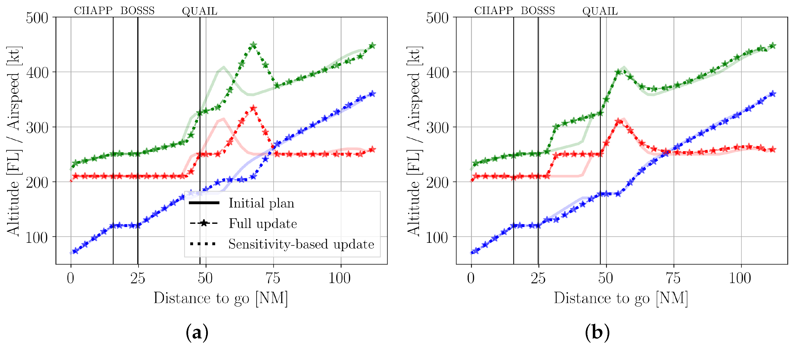
The initial (unperturbed) trajectory computed at the TOD for this illustrative example is shown in the two panels of Figure 3. The vector of parameters used to generate this trajectory was composed by the control points of the spline approximating the wind forecast data obtained from RAP (see Figure 2), the nominal initial state exposed in Section 4.3 and the CTA corresponding to the simulation for the same wind forecast and analysis. Figure 3 also shows the trajectories that would result from solving the rigorous NLP and a sensitivity-based update with perturbations in different elements of the parameters’ vector. Each panel of this figure corresponds to a different element of p: the wind perturbation was the difference between the control points of the splines approximating the RAP forecast and analysis data, δ c ; and the CTA perturbation, δ CTA , where the aircraft must arrive 30 s earlier than the FMS-calculated ETA for that forecast wind. It should be noted that each panel of Figure 3 shows only the results of a single trajectory update performed at τ 0 , after intentionally perturbing one element of p.
Figure 3 shows that the optimal trajectories resulting from sensitivity-based updates are almost identical to those obtained from solving a rigorous NLP optimization problem, even for large perturbations in the elements composing the parameters’ vector.
Figure 3a shows trajectory updates for perturbations in the control points of the spline approximating the wind profile. According to Figure 2, during the first part of the descent (from FL360 to FL200), the aircraft will encounter a tail wind that is significantly stronger than that reported by the initial wind forecast. Consequently, to keep the deviation from the CTA as small as feasible, the optimized trajectory update increased the aircraft’s descent rate between FL260 to FL200, thereby minimizing the impact of the significantly stronger than expected tailwind. To meet the speed constraint at QUAIL, the trajectory then leveled off the aircraft at FL200 to dissipate kinetic energy to 250 kts.
Figure 3b illustrates how the guidance strategy resolved the time error caused by the CTA being 30 s earlier than the original estimated time of arrival. The guidance strategy accomplished this by having the aircraft descend at a slightly faster rate to achieve and maintain the faster airspeed possible, while still meeting the path and terminal constraints for QUAIL and BOSSS listed in Table 1.

5.2. Illustrative Examples: Guidance Strategies

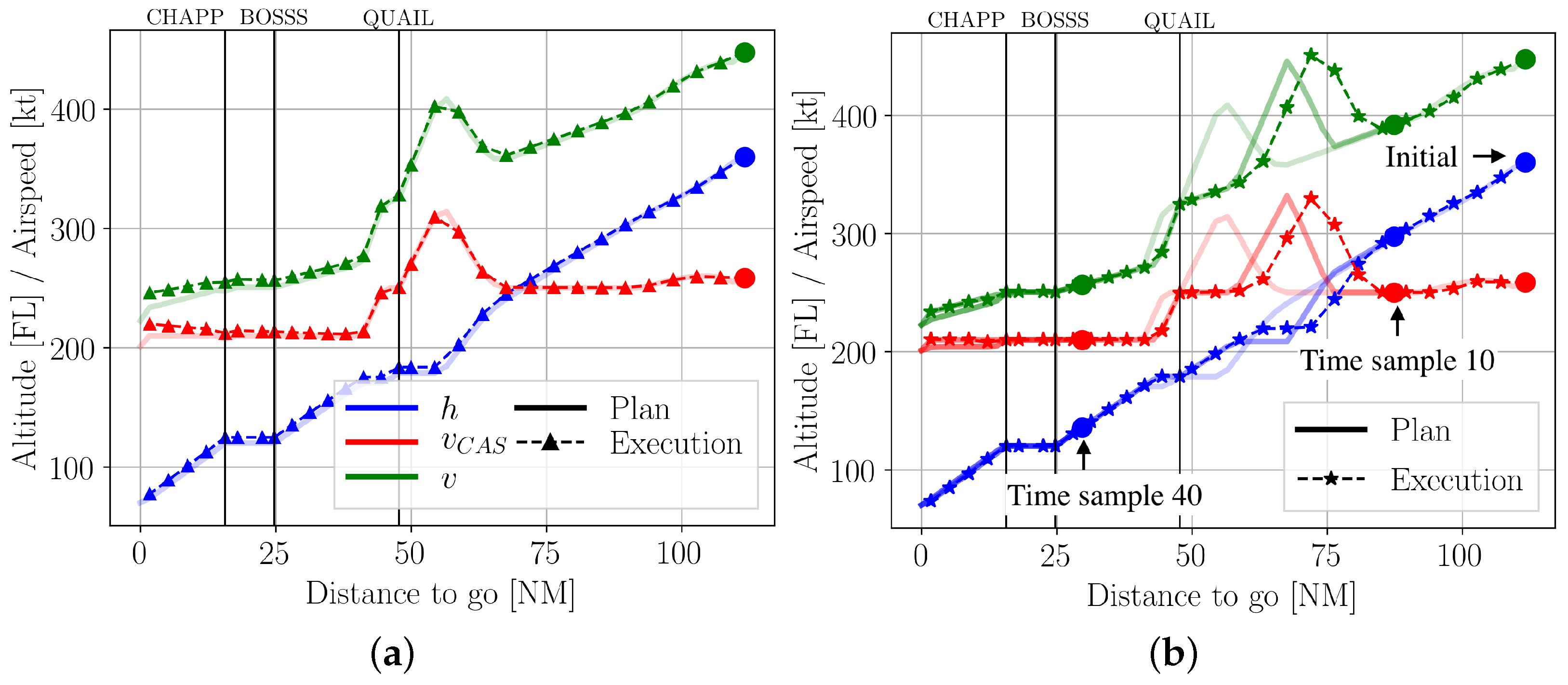
Using the same wind forecast and analysis as in the previous section, this section will describe the behavior of the NMPC guidance strategies considered in this experiment. Figure 4 shows the initially planned trajectory (computed at the TOD) and the executed trajectory, for the INMPC variant and for the open-loop strategy (OL). Results for the remaining NMPC strategies are not shown since the differences between them are small enough that they are difficult to visually observe in a plot.
The light solid lines in Figure 3 and Figure 4 are identical to each other, that is, the initially planned trajectory of the same run. Then, the slightly darker solid lines in Figure 4 represent the plans resulting from trajectory updates at two of the sixty time samples. These time samples, which were selected only for illustrative purposes, are Time sample 10 ( τ 10 ) and Time sample 40 ( τ 40 ) in the figure. The plans generated at the remaining time samples are not shown for the sake of clarity, even if being computed.
Before updating the trajectory at each time sample, the NMPC guidance system recalculates the control points of the spline that approximates the wind profile, based on the actual wind sensed at the current altitude. The wind profile used by the NMPC trajectory optimizer converges to the actual wind profile as wind measurements are collected during the execution of the descent. The impact of the wind forgetting function (or blending of actual sensed wind with forecast wind) is demonstrated in Figure 2 by the difference between the initial wind spline (forecast wind when the aircraft is at FL360 and TOD) and the wind spline at τ 10 (aircraft at approximately FL300).
It should be noted that the optimal control applied at each time sample is based on the best estimation of the wind profile at the current altitude. However, the actual wind conditions that the aircraft will encounter at lower altitudes are still unknown. Even if the control applied at each time sample is optimal for the estimated wind, it may be sub-optimal for the actual (unknown) wind conditions.

5.3. Aggregated Results

This section presents the results for the 4143 case studies per guidance strategy.

5.3.1. Time Error and Specific Energy Error Results

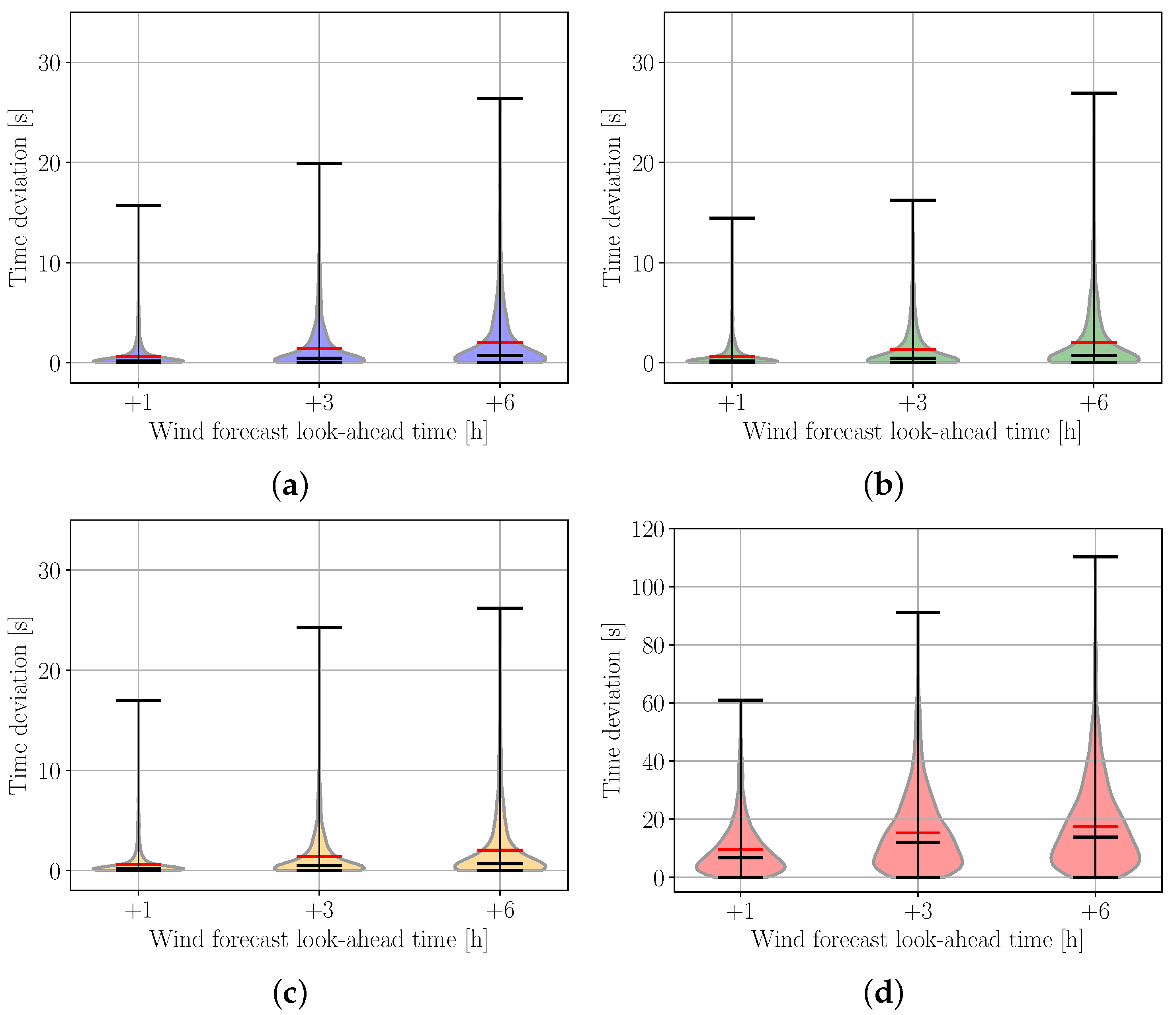
Figure 5 shows the absolute time error at the metering/merging fix (DYMON) as a function of the guidance strategy, and Figure 6 shows the specific energy ( E s ) (i.e., the energy divided by the aircraft weight) deviation at the metering fix as a function of the guidance strategy. The black horizontal line represents the median, the red horizontal line is the mean, and the whiskers extend out to the minimum and maximum values. Note that the y-axis of the plots within Figure 5 and within Figure 6 have fundamentally different scales, therefore if comparing NMPC to open-loop, care must be taken to draw the correct conclusion.
According to Figure 5, and as expected, the larger the look-ahead time of the wind forecast, the more time error (in absolute value) was observed, independently of the guidance strategy. The maximum time error (115 s) was realized using the open-loop guidance strategy with a wind forecast of +6 h. The median time error when using this guidance strategy with a wind forecast of +6 h was around 15 s. For a wind forecast of +1 h this value was reduced to 8 s. For the set of descents simulated with a wind forecast of +6 h, the distribution of time errors was concentrated in the range [ 0 , 60 ] s.
When using strategies based on NMPC, the time error was drastically reduced. For all case studies analyzed herein the time error was always lower than 27 s. The median time error for any of the NMPC guidance strategies was lower than 2 s for the set of descents simulated with a wind forecast of +6 h. In addition, the distribution of time errors was always concentrated in the range [ 0 , 10 ] s.
Similar results were observed for the specific energy error. According to Figure 6d, the metering fix could be achieved with specific energy errors up to 1800 ft by implementing the control of the initial optimal trajectory in open-loop. Conversely, guidance strategies based on NMPC achieved the metering/merging fix with negligible specific energy error, always lower than 150 ft and with a median value around 10 ft for a wind forecast of +6 h. In addition, the distribution of specific energy errors for the open-loop extends up to 1000 ft, while for any of the NMPC strategies this value is 75 ft.
Figure 5 and Figure 6 show that the performance of the SbNMPC in terms of energy and time errors is equivalent to that of INMPC and AsNMPC. Results agree with those shown in previous sections, where the trajectory updates based on parametric sensitivities were similar to those obtained by solving the rigorous NLP optimization problem.

5.3.2. Speed Brakes, Throttle and Fuel Results

The optimal control computed at each τ i could demand to modulate energy with the elevator or to add/remove energy to/from the system by means of additional thrust or speed brakes. Ideally, the NMPC optimizer will attempt to obtain an energy-neutral trajectory. In certain conditions with significant errors in the model parameters, however, energy modulation by means of elevator control may not be sufficient to obtain a solution satisfying all the constraints. In this case, the NMPC trajectory optimizer would calculate the optimal amount of energy to be added or removed in terms of fuel consumption and use of speed brakes such that all constraints are satisfied.
Table 2 shows the percentage of simulations in which the guidance system was able to execute the descent without applying speed brakes (independently of the thrust), without using additional thrust (independently of the speed brakes), and without neither applying speed brakes nor using additional thrust (the energy-neutral trajectories).
According to Table 2, in general the larger the forecast look-ahead time, the more chances the guidance system has to apply speed brakes and/or use additional thrust, independently of the guidance strategy. For instance, for a forecast look-ahead time of +1 h, the number of descents that could be executed using only elevator control to satisfy constraints is around 80%. For a forecast look-ahead of +6 h, this value is reduced to 67%. Again, results for the three NMPC variants compared in this paper are very similar.
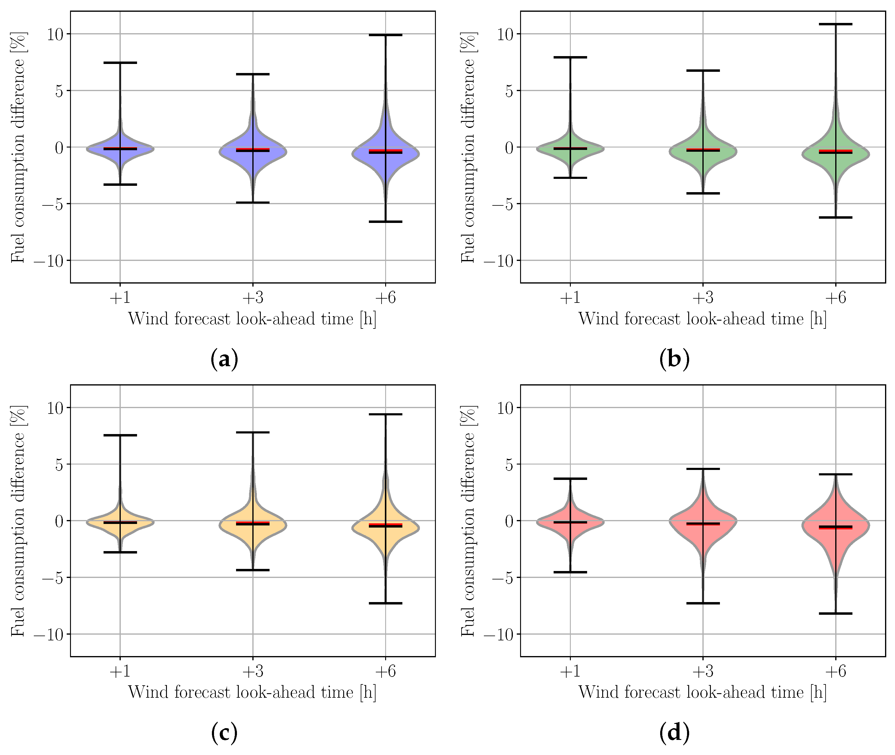
Figure 7 shows the difference in fuel consumption between the executed trajectory and that initially planned when receiving the CTA for each guidance strategy. Negative values indicate less fuel consumption, positive values indicate more fuel consumption.
Interestingly, Figure 7 shows that using any of the three NMPC guidance strategies the fuel burned during the execution is typically the same than that initially planned. In addition, Figure 7 illustrates that the maximum extra fuel consumption required to compensate potential time errors up to 115 s and specific energy errors up to 1800 ft is always lower than 10%. The key conclusion of Figure 7 is that NMPC strategies do not incur additional fuel burn compared to open-loop, yet enable the aircraft to conform to the constraints described in the previous sections.

5.3.3. Sensitivity to Wind Error

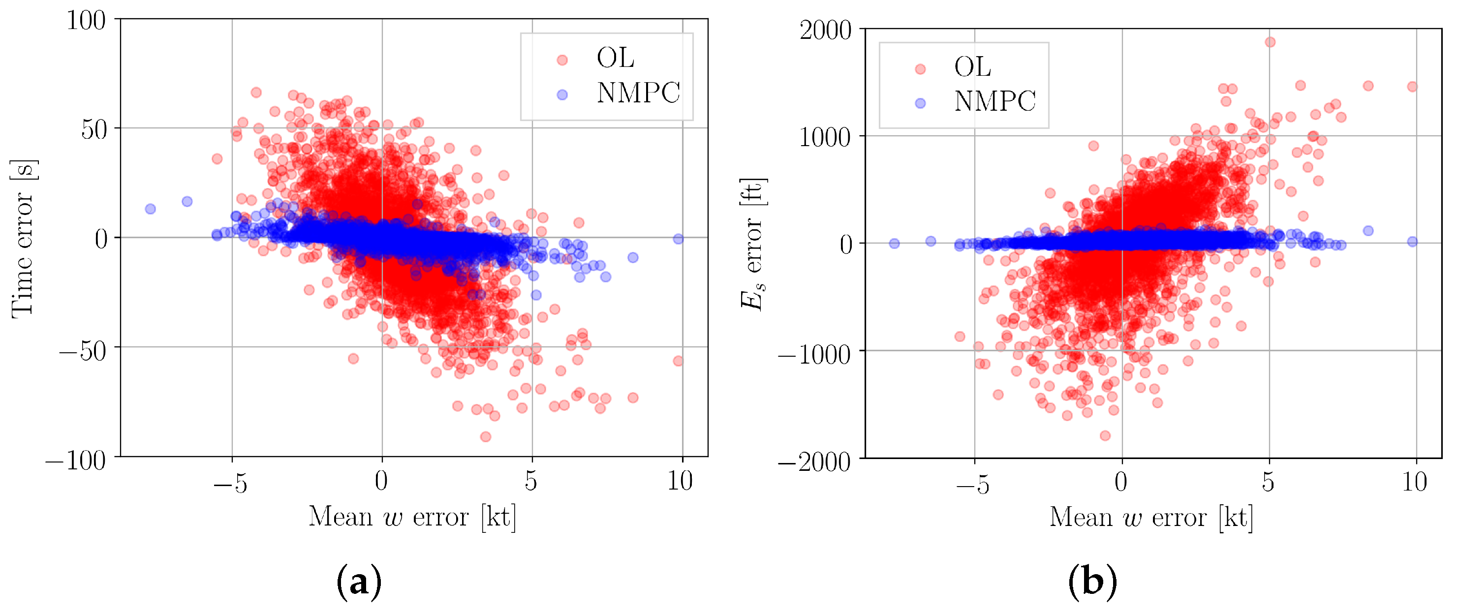
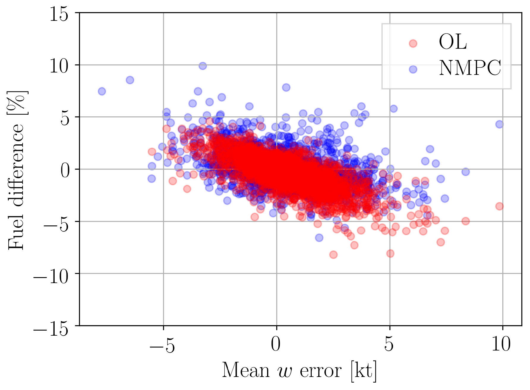
The previous section assessed the performance of three NMPC guidance strategies in the presence of errors in the longitudinal wind profile forecast, and compared the results with those of the open-loop execution. Figure 8 and Figure 9 show the correlation between the different metrics of the performance assessment and the mean longitudinal wind error, shown as w on the X-axis. The mean longitudinal wind error for each case study has been computed by averaging the longitudinal wind error of all sixty time samples. Positive values indicate more tail wind than initially expected, negative values manifest a stronger head wind if compared to the forecast. Each data point in these figures corresponds to a particular case study. In order to keep this figure simple, only the results for the open-loop and INMPC guidances are shown. Yet, it should be noted that results for the remaining NMPC strategies are very similar to those of the INMPC.
According to Figure 8a, and as expected, when executing the initial optimal control in open-loop, the time error at the metering/merging fix shows a strong, negative correlation with the mean longitudinal wind error, i.e., the stronger the unexpected head wind, the later the aircraft will arrive with respect to the CTA. Analogously, the specific energy error at the metering/merging fix (see Figure 8b) presents a strong, positive correlation with the mean longitudinal error, meaning that the stronger the unexpected head wind, the lower the energy of the aircraft will be at the metering/merging fix.
For the NMPC strategies, the time error appears to be weakly correlated with the mean longitudinal wind error; and the specific energy error is not correlated at all. The differences in the correlation patterns for the open-loop and NMPC guidance strategies are caused by the corrective actions performed by the latter, which repeatedly updates the optimal descent trajectory to satisfy the terminal constraints at the metering/merging fix while minimizing the environmental impact.
Figure 9 shows that the fuel consumption presents a negative correlation with the mean longitudinal wind error, meaning that the stronger the unexpected tail wind, the less thrust and fuel consumption are required if compared to the initial plan computed at the TOD. Remember that the open-loop strategy executes the initial control plan (i.e., thrust and flight path angle) without nullifying altitude nor speed deviations. For a given thrust value, however, the fuel flow changes with the altitude and the speed. Accordingly, the fuel consumption difference is caused by altitude and speed deviations from the initial trajectory plan. For the NMPC guidance strategies, these differences are also caused by trajectory updates that might modify the states and controls plans. For this reason, results for the NMPC guidance strategies show more dispersion.

6. Conclusions

To reduce aircraft fuel consumption and emissions during arrival operations without compromising airport throughput, the use of continuous descent operations (CDOs) with a controlled time of arrival (CTA) to a metering/merging fix has emerged as a potent tool to achieve these two objectives simultaneously. This paper compared three guidance strategies based on non-linear model predictive control (NMPC) to an open-loop baseline, in the presence of altitude, wind and time error, to determine the efficacy of each in meeting constraints of a CDO currently in use at a major US airport.
Of these, the sensitivity-based NMPC (SbNMPC) and advanced-step NMPC (AsNMPC) guidance strategies are explored as an alternative approach to reduce the computational intensity of the ideal NMPC (INMPC), without impacting the accuracy of the trajectory calculations required to meet the constraints established by the CDO and set by the CTA. An in-house flight simulator based on the performance model of the Airbus A320 was used to simulate 4143 descents for each guidance strategy. Each simulation used the path and terminal constraints of an existing arrival procedure, imposed a CTA, and injected a wind error through the use of published forecast winds for the trajectory planning and the corresponding actual winds for the execution.
Results indicate that, in terms of meeting the CDO and CTA constraints (speed, altitude, time), the SbNMPC and AsNMPC guidance strategies were operationally equivalent to the INMPC guidance strategy, and frequently the differences in fuel consumption, changes in throttle or speed brakes, or other errors were statistically insignificant as well. These are all strong indications that the simpler and faster parametric sensitivities approach are sufficient to achieve the same level of performance as the more rigorous non-linear programming optimization approach used by INMPC. The results also demonstrated that in the face of wind error and time error, all the NMPC-based guidance strategies were generally able to achieve the CDO and CTA constraints without requiring significant additional thrust or use of speed brakes. In terms of fuel consumption, descents using any of the NMPC all had a mean of essential 0% additional fuel consumption when compared to an open-loop descent. This is a very strong indication the NMPC guidance strategies were able to achieve, without incurring a fuel penalty, the CDO and CTA constraints where the open-loop strategy did not.
The results presented in this paper, however, are only valid for the Airbus A320, which nonetheless represents the vast majority of worldwide narrow-body commercial aircraft. It is worth noting that the Boeing 737, which has a similar performance to the A320, is the second most commonly used aircraft nowadays. Accordingly, the fuel consumption, specific energy, and time error figures presented in the paper are likely to be valid for a very large percentage of airliners currently in operations. Furthermore, the proposed planning and guidance algorithms are generic enough to consider different aircraft types by adopting the corresponding performance model. In future works, the figures presented herein must be compared with those of other aircraft types.
The accurate and robust achievement of CTA in descents is a key requirement for arrival managers (AMAN), which are decision support systems for air traffic control when sequencing and merging arrival traffic in terminal airspace. The results shown in this paper could become an important technical enabler for future FMS capable of advanced 4D trajectory negotiation and synchronization with enhanced AMAN systems, which would ultimately aim to maximize the number of executed CDOs, even during high peaks of incoming traffic. See for instance the research done in [36], where accurate CTA fulfillment is a key element to schedule traffic in a 4D trajectory synchronization paradigm based on tromboning procedures; or more recently in [37], where a novel methodology is proposed based on a pre-sequencing area used to assign CTA to all incoming traffic, followed by a dynamic-trajectories area designed to optimize the sequencing and merging operations.

Author Contributions

Conceptualization, R.D., X.P. and B.B.; methodology, R.D., X.P. and B.B.; software, R.D.; validation, R.D.; formal analysis, R.D., X.P. and B.B; investigation, R.D., X.P. and B.B.; data curation, R.D.; writing—original draft preparation, R.D., X.P. and B.B.; writing—review and editing, R.D., X.P. and B.B.; visualization, R.D.; supervision, X.P. and B.B.; project administration, X.P. and B.B. All authors have read and agreed to the published version of the manuscript.

Funding

This research was funded by “la Caixa” Foundation: International mobility grant for students.

Institutional Review Board Statement

Not applicable.

Informed Consent Statement

Not applicable.

Data Availability Statement

Publicly available weather datasets were analyzed in this study. This data can be found here: https://ruc.noaa.gov/.

Conflicts of Interest

The authors declare no conflict of interest.

References

  1. Bryson, A.E.; Ho, Y. Applied Optimal Control: Optimization, Estimation, and Control; Taylor and Francis Group: New York, NY, USA, 1975. [Google Scholar]
  2. González-Arribas, D.; Soler, M.; Sanjurjo-Rivo, M. Robust Aircraft Trajectory Planning Under Wind Uncertainty Using Optimal Control. J. Guid. Control. Dyn. 2018, 41, 673–688. [Google Scholar] [CrossRef] [Green Version]
  3. Kamo, S.; Rosenow, J.; Fricke, H.; Soler, M. Robust CDO Trajectory Planning under Uncertainties in Weather Prediction. In Proceedings of the the 13th USA/Europe Air Traffic Management Research and Development Seminar, Saclay, France, 17–19 June 2019. [Google Scholar]
  4. Dalmau, R.; Prats, X.; Verhoeven, R.; Bussink, F.J.L.; Heesbeen, B. Performance comparison of guidance strategies to accomplish RTAs during a CDO. In Proceedings of the 36th AIAA/IEEE Digital Avionics Systems Conference (DASC), St. Petersburg, FL, USA, 17–21 September 2017. [Google Scholar] [CrossRef] [Green Version]
  5. de Jong, P.M.A.; de Gelder, N.; Verhoeven, R.; Bussink, F.J.L.; Kohrs, R.; van Paassen, M.M.; Mulder, M. Time and Energy Management During Descent and Approach: Batch Simulation Study. J. Aircr. 2014, 52, 190–203. [Google Scholar] [CrossRef]
  6. Diehl, M.; Ferreau, H.J.; Haverbeke, N. Efficient Numerical Methods for Nonlinear MPC and Moving Horizon Estimation Problem Formulation. In Nonlinear Model Predictive Control; Springer: Berlin/Heidelberg, Germany, 2008; pp. 391–417. [Google Scholar] [CrossRef] [Green Version]
  7. Dalmau, R.; Verhoeven, R.; De Gelder, N.; Prats, X. Performance comparison between TEMO and a typical FMS in presence of CTA and wind uncertainties. In Proceedings of the 35th AIAA/IEEE Digital Avionics Systems Conference (DASC), Sacramento, CA, USA, 25–29 September 2016. [Google Scholar] [CrossRef] [Green Version]
  8. Weitz, L.A.; Bai, X. Using Model Predictive Control for Trajectory Optimization and to Meet Spacing Objectives. In Proceedings of the AIAA Guidance, Navigation, and Control Conference, Kissimmee, FL, USA, 8–12 January 2018. [Google Scholar]
  9. Ru, P.; Subbarao, K. Nonlinear Model Predictive Control for Unmanned Aerial Vehicles. Aerospace 2017, 4, 31. [Google Scholar] [CrossRef]
  10. Mothes, F. Trajectory Planning in Time-Varying Adverse Weather for Fixed-Wing Aircraft Using Robust Model Predictive Control. Aerospace 2019, 6, 68. [Google Scholar] [CrossRef] [Green Version]
  11. Suwartadi, E.; Kungurtsev, V.; Jäschke, J. Sensitivity-Based Economic NMPC with a Path-Following Approach. Processes 2017, 5, 8. [Google Scholar] [CrossRef] [Green Version]
  12. Kim, T.J.; Hull, D.G. Optimal control design that accounts for model mismatch errors. In Proceedings of the AAS/MAA Space Flight Mechanics Meeting, Albuquerque, New Mexico, 13–16 February 1995. [Google Scholar]
  13. Zavala, V.M.; Biegler, L.T. The advanced-step NMPC controller: Optimality, stability and robustness. Automatica 2009, 45, 86–93. [Google Scholar] [CrossRef]
  14. Wetzel, T.A. Development of a Finite Difference Neighboring Optimal Control Law and Application to the Optimal Landing of a Reusable Launch Vehicle. Ph.D. Thesis, Iowa State University, Ames, IA, USA, 1996. [Google Scholar]
  15. Pesch, H.J. Numerical computation of neighboring optimum feedback control schemes in real-time. Appl. Math. Optim. 1979, 5, 231–252. [Google Scholar] [CrossRef]
  16. Würth, L.; Hannemann, R.; Marquardt, W. An Efficient Strategy for Real-Time Dynamic Optimization based on Parametric Sensitivities. IFAC Proc. Vol. 2008, 41, 1928–1933. [Google Scholar] [CrossRef] [Green Version]
  17. Würth, L.; Hannemann, R.; Marquardt, W. Neighboring-extremal updates for nonlinear model-predictive control and dynamic real-time optimization. J. Process. Control. 2009, 19, 1277–1288. [Google Scholar] [CrossRef]
  18. Wolf, I.J.; Marquardt, W. Fast NMPC schemes for regulatory and economic NMPC—A review. J. Process. Control. 2016, 44, 162–183. [Google Scholar] [CrossRef]
  19. Dalmau, R.; Baxley, B.; Prats, X. Fast sensitivity-based optimal trajectory updates for descent operations subject to time constraints. In Proceedings of the 37th IEEE/AIAA Digital Avionics Systems Conference (DASC), London, UK, 23–27 September 2018. [Google Scholar] [CrossRef] [Green Version]
  20. Betts, J.T. Practical Methods for Optimal Control and Estimation Using Nonlinear Programming, 2nd ed.; SIAM: Philadelphia, PA, USA, 2010; p. 434. [Google Scholar] [CrossRef]
  21. Dalmau, R. Optimal Trajectory Management for Aircraft Descent Operations Subject to Time Constraints. Ph.D. Thesis, Technical University of Catalonia (UPC), Barcelona, Spain, 2019. [Google Scholar]
  22. Jäschke, J.; Yang, X.; Biegler, L.T. Fast economic model predictive control based on NLP-sensitivities. J. Process. Control. 2014, 24, 1260–1272. [Google Scholar] [CrossRef]
  23. Kadam, J.V.; Marquardt, W. Sensitivity-Based Solution Updates in Closed-Loop Dynamic Optimization. IFAC Proc. Vol. 2004, 37, 947–952. [Google Scholar] [CrossRef]
  24. Gros, S.; Srinivasan, B.; Chachuat, B.; Bonvin, D. Neighbouring-extremal control for singular dynamic optimisation problems. Part I: Single-input systems. Int. J. Control. 2009, 82, 1099–1112. [Google Scholar] [CrossRef]
  25. Clarke, J.P.B.; Ho, N.T.; Ren, L.; Brown, J.A.; Elmer, K.R.; Zou, K.F.; Hunting, C.; McGregor, D.L.; Shivashankara, B.N.; Tong, K.; et al. Continuous descent approach: Design and flight test for Louisville international airport. J. Aircr. 2004, 41, 1054–1066. [Google Scholar] [CrossRef]
  26. de Boor, C. On calculating with B-splines. J. Approx. Theory 1972, 6, 50–62. [Google Scholar] [CrossRef] [Green Version]
  27. de Jong, P.M.A.; van der Laan, J.J.; Veld, A.C.; van Paassen, M.M.; Mulder, M. Wind-Profile Estimation Using Airborne Sensors. J. Aircr. 2014, 51, 1852–1863. [Google Scholar] [CrossRef]
  28. Poles, D.; Nuic, A.; Mouillet, V. Advanced aircraft performance modelling for ATM: Analysis of BADA model capabilities. In Proceedings of the 29th Digital Avionics Systems Conference (DASC), Salt Lake City, UT, USA, 3–7 October 2010. [Google Scholar] [CrossRef]
  29. Hindmarsh, A.C.; Brown, P.N.; Grant, K.E.; Lee, S.L.; Serban, R.; Shumaker, D.E.; Woodward, C.S. SUNDIALS: Suite of nonlinear and differential/algebraic equation solvers. ACM Trans. Math. Softw. 2005, 31, 363–396. [Google Scholar] [CrossRef]
  30. Dalmau, R.; Melgosa, M.; Prats, X. pyBADA: Easy BADA integration in python for rapid prototyping. In Proceedings of the 8th SESAR Innovation Days (SID), Salzburg, Austria, 3–6 December 2018. [Google Scholar]
  31. Airbus. Getting to Grips with the Cost Index; Technical Report; Airbus Flight Operations Support & Line Assistance: Blagnac, France, 1998. [Google Scholar]
  32. Dalmau, R.; Prats, X. Controlled time of arrival windows for already initiated energy-neutral continuous descent operations. Transp. Res. Part C 2017, 85, 334–347. [Google Scholar] [CrossRef] [Green Version]
  33. Andersson, J.; Akesson, J.; Diehl, M. Dynamic optimization with CasADi. In Proceedings of the IEEE Conference on Decision and Control, Maui, HI, USA, 10–13 December 2012; pp. 681–686. [Google Scholar] [CrossRef]
  34. Andersson, J.; Gillis, J.; Horn, G.; Rawlings, J.B.; Diehl, M. CasADi—A software framework for nonlinear optimization and optimal control. Math. Program. Comput. 2019, 11, 1–36. [Google Scholar] [CrossRef]
  35. Gill, P.E.; Murray, W.; Saunders, M.A. SNOPT: An SQP algorithm for large-scale constrained optimization. Soc. Ind. Appl. Math. 2005, 47, 99–131. [Google Scholar] [CrossRef]
  36. Sáez, R.; Prats, X.; Polishchuk, T.; Polishchuk, V. Traffic synchronization in terminal airspace to enable continuous descent operations in trombone sequencing and merging procedures: An implementation study for Frankfurt airport. Transp. Res. Part C 2020, 121, 102875. [Google Scholar] [CrossRef]
  37. Sáez, R.; Polishchuk, T.; Schmidt, C.; Hardell, H.; Smetanová, L.; Polishchuk, V.; Prats, X. Automated sequencing and merging with dynamic aircraft arrival routes and speed management for continuous descent operations. Transp. Res. Part C 2021, 132, 103402. [Google Scholar] [CrossRef]
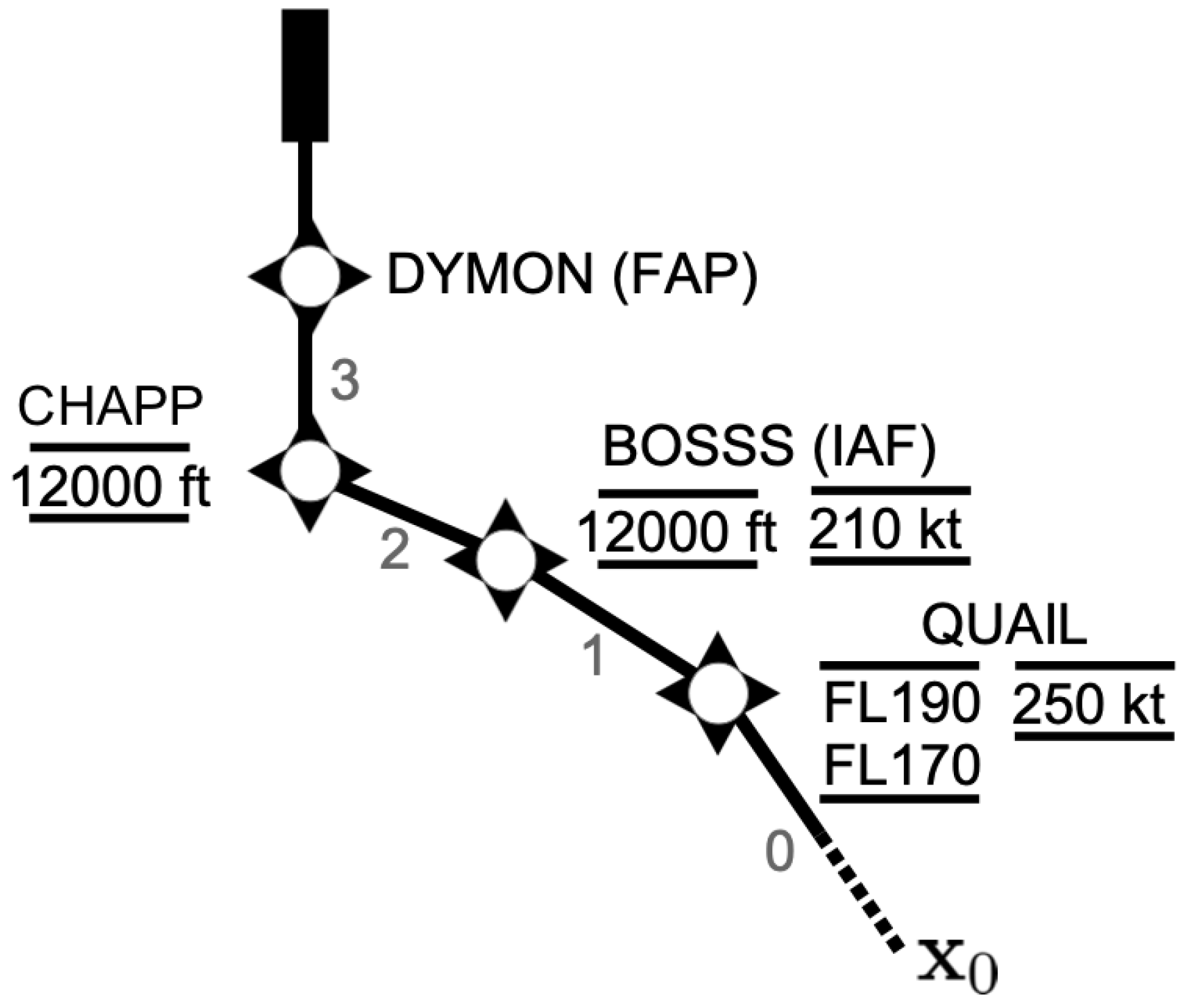
Figure 1. BOSSS TWO standard arrival procedure.
Aerospace 08 00377 g001
Figure 2. RAP wind forecast and analysis (21 April 2018 00:00 with a look-ahead time of +1 h).
Aerospace 08 00377 g002
Figure 3. Optimal trajectory updates for perturbations in the parameters vector (21 April 2018 00:00 with a look-ahead time of +1 h). (a) δ c (actual minus forecast of Figure 2). (b) δ CTA = 30 s .
Aerospace 08 00377 g003
Figure 4. Planned and executed trajectories by control method (21 April 2018 00:00 with a look-ahead time of +1 h). (a) Open-loop. (b) INMPC.
Aerospace 08 00377 g004
Figure 5. Time deviation at the metering/merging fix. (a) NMPC. (b) SbNMPC. (c) AsNMPC. (d) Open-loop.
Aerospace 08 00377 g005
Figure 6. Specific energy deviation at the metering/merging fix. (a) NMPC. (b) SbNMPC. (c) AsNMPC. (d) Open-loop.
Aerospace 08 00377 g006
Figure 7. Fuel consumption difference with respect to the initial plan. (a) NMPC. (b) SbNMPC. (c) AsNMPC. (d) Open-loop.
Aerospace 08 00377 g007
Figure 8. Time and specific energy error at the metering/merging fix. (a) Time error. (b) Specific energy error.
Aerospace 08 00377 g008
Figure 9. Fuel consumption difference with respect to initial plan.
Aerospace 08 00377 g009
Table 1. Definition of the phases and associated constraints for the BOSSS TWO procedure.
jDescription b j in φ j eq ϑ j in ϑ j eq
0TOD-QUAIL M ( h , V ) MMO v C A S ( v , h ) VMO 250 kt v C A S ( v , h ) - FL 170 h h FL 190 v C A S ( v , h ) 250 kt
1QUAIL-BOSSS v C A S ( v , h ) 250 kt 210 kt v C A S ( v , h ) -- v C A S ( v , h ) 210 kt h 12 , 000 ft
2BOSSS-CHAPP v C A S ( v , h ) 210 kt GD v C A S ( v , h ) h ˙ --
3CHAPP-DYMON v C A S ( v , h ) 210 kt GD v C A S ( v , h ) --
Table 2. Energy-neutral trajectories per guidance strategy.
Guidance StrategyWithout Speed Brakes Without Additional Thrust Energy-Neutral
+1+3+6+1+3+6+1+3+6
INMPC98.393.790.082.175.675.580.670.367.0
SbNMPC98.393.289.281.977.476.680.571.367.4
AsNMPC98.693.289.982.076.376.780.970.568.4
Publisher’s Note: MDPI stays neutral with regard to jurisdictional claims in published maps and institutional affiliations.