Optimal Guidance Law with Impact-Angle Constraint and Acceleration Limit for Exo-Atmospheric Interception

Abstract

This paper aims to develop an optimal guidance law for exo-atmospheric interception, in which impact-angle constraint and acceleration limit are considered. Firstly, an optimal control problem with constraints on terminal miss and impact-angle is formulated, in which the control energy performance index is weighted by a power function of the time-to-go. The closed-loop guidance command, which is expressed as a linear combination of zero-effort miss distance and the zero-effort angle error, is derived using a traditional order reduction transformation. Then, an analytical solution to the maximal acceleration during the flight is obtained by analyzing the boundary points and critical points of the guidance command curve. It is found that the maximal acceleration is a function of the weighted gain in the performance index. Therefore, the maximal acceleration can be efficiently limited by using the variable weighted gain. Furthermore, the relationship between the total control energy and the weighted gain is studied. As a result, a systematic method is proposed for selecting the weighted gain so as to meet the constraint of the acceleration while the total control energy is minimal. Nonlinear simulations have been carried out to test the performance of the proposed method. The results show that this method performs well in intercepting the maneuvering target with a negligible miss distance and intercept angle error. And it can tolerate a stricter acceleration limit in comparison with the typical method.

1. Introduction

The terminal guidance law, which has direct influence on kill efficiency, is immensely important for the weapon system. During terminal attack, the achievement of a proper impact angle is an important goal of homing systems. Using impact-angle-control, the missile is capable of attacking a weak spot of the target to maximize warhead effectiveness and ensure a high kill probability [1,2]. In addition, the acceleration limit is another crucial constraint on homing missiles, which will lead to large miss-distance and impact angle error if the acceleration saturation occurs near the target.

Guidance law design with specific impact direction has been a hot topic during the past four decades. As an application of optimal control theory, Bryson and Ho [3] have proposed the optimal solution to the simple rendezvous problem with terminal constraints on the lateral position and velocity. In [4], a similar formulation was used to derive a linear quadratic optimal guidance law and linear quadratic differential game-based laws for maneuvering target scenarios. These two formulations can be utilized to impose a terminal intercept angle by selecting the ratio between the relative terminal velocity and the closing speed. Kim and Grider [5] first proposed an optimal guidance law to ensure the impact angle for a reentry vehicle, which pursues a fixed or slowly moving ground target. In [6], York and Pastrick further improved the guidance law presented in [5], in which the lag in the autopilot is considered. The resulting guidance law was applied to an air defense interceptor in [7]. In [8], a generalized form of energy minimization optimal guidance law was proposed for satisfying the impact-angle constraints. Song et al. [9] have studied an optimal impact angle guidance law for varying velocity missiles against a maneuvering ship. Shaferman [10] derived two impact angle control guidance laws based on the optimal control and differential game theory for an evasive maneuvering target. An optimal control planar interception law against maneuvering targets with known trajectories was devised in [11]. A terminal body angle control guidance law considering the angle-of-attack dynamics was developed in [12]. It is noted that the abovementioned optimal guidance laws are all based on a constant weighted performance index, which results in the weak ability of the trajectory shaping. And the terminal acceleration cannot be guaranteed to be zero, which possibly increases the miss-distance.

In order to address this drawback, Ryoo [13] proposed a time-to-go weighted optimal guidance with zero terminal acceleration because the weighting of cost infinitely increases as the time-to-go approaches zero. Ohlmeyer [14,15] proposed an optimal guidance law with a weighted gain specified by the user, called Generalized Vector Explicit Guidance, which improves the ability to shape the trajectory and achieves the impact-angle constraint. He [16] investigated a similar guidance law which considers the influence of the gravity and thrust in the exo-atmospheric interception engagement. Lee [17] further developed a generalized optimal guidance law with arbitrary weighted function to satisfy the impact-angle constraint. By considering the penalty term regarding the miss distance and intercept angle weighted by hyperbolic tangent functions in the performance index, Xiong [18] proposed a new optimal guidance law, of which the guidance performance was less affected by the time-varying speed. Li [19] further designed a unified optimal impact angle guidance law with the energy consumption weighted by an arbitrary positive function, which can adapt to different types of interceptors and targets. In addition to the guidance law based on the optimal control theory, biased proportional navigation [20,21,22,23,24] and sliding-mode guidance law [25,26,27,28,29] can also realize the impact with a specified angle. However, all these guidance laws do not consider the acceleration limit, which possibly leads to large miss-distance and impact angle error if the acceleration saturation occurs near the target.

In order to limit acceleration, Rusnak [30] and Hexner [31] directly solved the optimal control problem with control constraint, which leads to a significantly complicated solution. Weiss [32] introduced a new class of optimal guidance law in which a special performance index penalizing the variability of the guidance command is used, and therefore, an additional design parameter can be profitably used to avoid acceleration saturation. Although the acceleration limit is considered in this research, the impact-angle cannot be guaranteed. This is due to the fact that if the constraint of impact-angle is considered simultaneously, the solved guidance command is extremely complex and even cannot be solved analytically.

In this paper, an optimal guidance law with constraint on the impact-angle and acceleration limit is proposed. Firstly, an impact-angle constrained optimal guidance law (IACOGL) with a variable weighted gain is formulated. The closed-loop guidance command can be expressed as a linear combination of zero-effort miss distance (ZEM) and the zero-effort angle error (ZEAE). Then, we analyze the extreme value of the guidance command curve and derive the closed-form function between the maximum of guidance command with the weighted gain. Therefore, the maximal acceleration can be efficiently limited by using the variable weighted gain. Furthermore, the relationship between the total control energy and the weighted gain is studied. Finally, a systematic method to select the optimal weighted gain, which minimizes the total control energy and keeps the acceleration within the constraint, is proposed. The greatest difference from the previous works is that the proposed method is able to avoid acceleration saturation by choosing the appropriate weighted gain in an analytical manner, while having optimal performance for the guidance command. Several numerical simulations are carried out to evaluate the performance of the proposed method. The results show that this method performs well in intercepting the maneuvering target with the impact angle constraint and acceleration limit.

The remainder of this paper is organized as follows: In Section 2, the mathematical models used for the guidance law derivation and simulation are presented. Section 3 derives the time-to-go weighted optimal guidance law with constraint on impact-angle. Section 4 provides the derivation process on the maximum of guidance command and the total maneuvering energy. After which, a method used to select the weighted gain to avoid the acceleration saturation is also presented in Section 4. Finally, nonlinear simulations are carried out to evaluate the performance of the proposed law.

2. Model Formulation

Consider a planar engagement geometry for a maneuvering target shown in Figure 1. Here, $X_I-O_I-Y_I$ is a Cartesian inertial reference frame. We denote the missile and target by the subscripts M and T, respectively. The velocity, acceleration, and flight-path angles are denoted by $V$, $a$ and $\gamma$, respectively. It is assumed that the velocity of missile and target for guidance law derivation is constant. The range between the adversaries is $r$, and $\lambda$ is the angle between the line of sight (LOS) and the $X_I$ axis. The $X_R$ axis, aligned with the initial LOS, is denoted for linearization. The relative displacement between the target and the missile normal to this axis is $\xi$. The intercept angle between missile and angle is defined as ${\gamma }_I={\gamma }_T+{\gamma }_M$, which is required to be a given value ${\gamma }_f^c$ at the intercept time.

From Figure 1, the equations of relative motion between missile and target are given by

$$\dot{r}=-\left[V_T\cos \left({\gamma }_T+\lambda \right)+V_M\cos \left({\gamma }_M-\lambda \right)\right]$$

(1)

$$\dot{\lambda }=\left[-V_M\sin \left({\gamma }_M-\lambda \right)+V_T\sin \left({\gamma }_T+\lambda \right)\right]/r$$

(2)

And, due to the existence of acceleration and gravitational effect, the flight-path angle and velocity of the missile as well as the target evolve according to

$${\dot{\gamma }}_M=\left[a_M\cos \left({\gamma }_M-\lambda \right)-g_M\cos {\gamma }_M\right]/V_M$$

(3)

$${\dot{V}}_M=a_M\sin \left({\gamma }_M-\lambda \right)-g_M\sin {\gamma }_M$$

(4)

where, $g_M$ stands for the gravitational acceleration of the missile. Similarly, due to the gravitational effect, the flight-path angle and velocity of target evolve according to

$${\dot{\gamma }}_T=-g_T\cos {\gamma }_T/V_T$$

(5)

$${\dot{V}}_T=-g_T\sin {\gamma }_T$$

(6)

where, $g_T$ is the gravitational acceleration of the target. $g_M$ and $g_T$ are assumed as a constant $g$ because the duration of the terminal guidance phase is typically very short.

It is assumed that the missile’s closed-loop dynamics can be represented by the following first-order system:

$${\dot{a}}_M=\left(u-a_M\right)/T$$

(7)

where, $u$ is the guidance command, $T$ is the time constant of the missile’s dynamics.

As was done in [10], the derivation of the guidance law in this paper will be performed based on a linearized model. In the linear model, the kinematics equations of $\xi$ and ${\gamma }_I$ are

$$\ddot{\xi }=-a_M$$

(8)

$${\dot{\gamma }}_I=\left(k_M{a}_M+\Delta g_{\gamma }\right)/V_M$$

(9)

where, $k_M=\cos \left({\gamma }_M-\lambda \right)$ and $\Delta g_{\gamma }=-g\left(\cos {\gamma }_M+\cos {\gamma }_T{V}_M/V_T\right)$. In the derivation of the guidance law, $V_M$, $k_M$, and $\Delta g_{\gamma }$ are regarded as the constants and will be updated in each guidance step. The state vector of the linearized problem is defined as

$$x={\left[\begin{array}{ccc}\xi & \dot{\xi }& {\gamma }_I\end{array}\right]}^T$$

(10)

The matrix form of the kinematic equations is

$$\dot{x}=Ax+Bu+C$$

(11)

where

$$A=\left[\begin{array}{ccc}0& 1& 0\\ 0& 0& 0\\ 0& 0& 0\end{array}\right],B=\left[\begin{array}{c}0\\ -1\\ k_M/V_M\end{array}\right],C=\left[\begin{array}{c}0\\ 0\\ \Delta g_{\gamma }/V_M\end{array}\right]$$

(12)

3. Derivation of IACOGL

In this section, an impact-angle constraint guidance law with a variable weighted gain is derived on the foundation of optimal control theory. Now, let us consider the following optimal control problem: Find $u\left(t\right)$ that minimizes defined by

$$J=\frac{1}{2}{\displaystyle {\int }_{t_0}^{t_f}{u}^2/t_{go}^{N}dt}$$

(13)

subject to (11) and terminal constraints given by

$$\begin{array}{cc}\xi \left(t_f\right)=0,& {\gamma }_I\left(t_f\right)-{\gamma }_f^c=0\end{array}$$

(14)

where, $t_{go}=t_f-t$ is the time-to-go; $N$ is weighted gain, which is the shaping parameter of the guidance command.

3.1. Order Reduction Transformation

Bryson and Ho [3] introduced a transformation enabling reducing an optimal control problem’s order, which is denoted as terminal projection and can be used to simplify the derivation. This transformation can be easily applied to the resulting optimal control problem in previous section.

As was done in [10], let us define a new state vector $Z\left(t\right)$ that satisfies

$$Z\left(t\right)=D\Phi \left(t_f,t\right)x\left(t\right)+D{\displaystyle {\int }_t^{t_f}\Phi \left(t_f,\tau \right)Cd\tau }-D{x}_f^c$$

(15)

where $\Phi \left(t_f,t\right)$ is the transition matrix associated with Equation (11), $x_f^c$ indicates the terminal constraint of $x\left(t\right)$, and $D$ is a constant matrix

$$D=\left[\begin{array}{cccc}1\hfill & 0\hfill & 0\hfill & {\left[0\right]}_{1\times n}\hfill \\ 0\hfill & 0\hfill & 1\hfill & {\left[0\right]}_{1\times n}\hfill \end{array}\right]$$

(16)

Since

$$\dot{\Phi }\left(t_f,t\right)=-\Phi \left(t_f,t\right)A$$

(17)

the time derivative of the new state vector $Z\left(t\right)$ is

$$\dot{Z}=D\left[\dot{\Phi }\left(t_f,t\right)x+\Phi \left(t_f,t\right)\dot{x}\right]-D\Phi \left(t_f,t\right)C=D\Phi \left(t_f,t\right)Bu=\left[\begin{array}{c}{\phi }_{\xi }\left(t_{go}\right)\\ {\phi }_{\gamma }\left(t_{go}\right)\end{array}\right]u$$

(18)

which is state independent and only the function of the guidance command $u$. The terminal value of $Z\left(t\right)$ can be expressed using (15) as

$$Z\left(t_f\right)=D\left[x\left(t_f\right)-x_f^c\right]={\left[\begin{array}{cc}\xi \left(t_f\right),& {\gamma }_I\left(t_f\right)-{\gamma }_f^c\end{array}\right]}^T$$

(19)

It is obvious that $Z\left(t_f\right)$ should be zeros. Then, using these new variables, the augmented cost function can be written as

$$\overline{J}={\upsilon }_1{Z}_1\left(t_f\right)+{\upsilon }_2{Z}_2\left(t_f\right)+\frac{1}{2}{\displaystyle {\int }_{t_0}^{t_f}{u}^2/t_{go}^{N}dt}$$

(20)

where, ${\upsilon }_1$ and ${\upsilon }_2$ are Lagrange multipliers;$Z_1\left(t_f\right)$ and $Z_2\left(t_f\right)$ are the first and second variables of $Z\left(t_f\right)$.

Note that, besides reducing the order of the problem, the two variables of the new state vector $Z\left(t\right)$ have an important physical meaning. $Z_1\left(t\right)$ is zero-effort miss distance (ZEM), and $Z_2\left(t\right)$ is zero-effort angle error (ZEAE), respectively referring to the miss distance and the impact-angle error if, from the current time onward, the missile will not apply any control.

3.2. Closed-Loop Optimal Guidance Command

According to the theory of optimal control, the Hamiltonian of the problem is

$$H=\frac{1}{2}{u}^2/t_{go}^N+{\lambda }_1{\phi }_{\xi }\left(t_{go}\right)u+{\lambda }_2{\phi }_{\gamma }\left(t_{go}\right)u$$

(21)

where ${\lambda }_1$ and ${\lambda }_2$ are co-state variables, respectively. Due to the order reduction transformation, the time derivative of the zero-effort variables is state independent, and therefore the adjoint equations can be presented in a simplified manner.

$$\left\{\begin{array}{c}{\dot{\lambda }}_1=-\partial H/\partial Z_1=0\\ {\dot{\lambda }}_2=-\partial H/\partial Z_2=0\end{array}\right.$$

(22)

Then we can obtain the co-state variables:

$$\left\{\begin{array}{c}{\lambda }_1\left(t\right)={\lambda }_1\left(t_f\right)={\upsilon }_1\hfill \\ {\lambda }_2\left(t\right)={\lambda }_2\left(t_f\right)={\upsilon }_2\hfill \end{array}\right.$$

(23)

For obtaining an analytic solution for the guidance command, it is assumed that the dynamics of missile are lag-free. Therefore, the time derivatives of the $Z_1$ and $Z_2$ are simplified as

$$\left\{\begin{array}{l}{\dot{Z}}_1={\phi }_{\xi }\left(t_{go}\right)u=-t_{go}u\hfill \\ {\dot{Z}}_2={\phi }_{\gamma }\left(t_{go}\right)u=u/{V^{\prime }}_M\hfill \end{array}\right.$$

(24)

where ${V^{\prime }}_M=V_M/k_M$. Therefore, the optimal guidance command for the missiles, which satisfy

$$u^{\ast }={\arg }_u\min H$$

(25)

are

$$\partial H/\partial u=0\Rightarrow u^{\ast }\left(t\right)={\lambda }_1{t}_{go}^{N+1}-{\lambda }_2{t}_{go}^N/{V^{\prime }}_M$$

(26)

Substituting (23) into (26) and integrating from $t$ to $t_f$ yields the following two coupled algebraic equations:

$$\begin{array}{l}{Z}_1\left(t_f\right)=Z_1\left(t\right)-{\upsilon }_1\frac{t_{go}^{N+3}}{N+3}+{\upsilon }_2\frac{t_{go}^{N+2}}{\left(N+2\right){V^{\prime }}_M}=0\\ Z_2\left(t_f\right)=Z_2\left(t\right)+{\upsilon }_1\frac{t_{go}^{N+2}}{\left(N+2\right){V^{\prime }}_M}-{\upsilon }_2\frac{t_{go}^{N+1}}{\left(N+1\right){V^{\prime }}_M^2}=0\end{array}$$

(27)

Solving ${\upsilon }_1$, ${\upsilon }_2$ and substituting the solution into (26), the optimal guidance command [10] is

$$u^{\ast }\left(t\right)=\frac{N_{ZEM}}{t_{go}^2}{Z}_1\left(t\right)+N_{ZEAE}\frac{{V^{\prime }}_M}{t_{go}}{Z}_2\left(t\right)$$

(28)

where, $N_{ZEM}$ and $N_{ZEAE}$ are the navigation gains, which are expressed as

$$\begin{array}{l}{N}_{ZEM}=\left(N+2\right)\left(N+3\right)\\ N_{ZEAE}=\left(N+1\right)\left(N+2\right)\end{array}$$

(29)

And the new states $Z_1$ and $Z_2$ can be expressed using state $x$ as

$$\begin{array}{l}{Z}_1\left(t\right)=\xi +\dot{\xi }{t}_{go}\\ Z_2\left(t\right)=\Delta g_{\gamma }{t}_{go}/V_M+{\gamma }_I-{\gamma }_f^c\end{array}$$

(30)

For the guidance law implementation, the time-to-go must be estimated. It can be approximated simply by

$$t_{go}=-r/\dot{r}$$

(31)

If the more accurate $t_{go}$ estimation is needed, the method presented in [8] can be adopted.

It is found that the command of the proposed guidance law is expressed as a linear combination of zero-effort miss distance and the zero-effort angle error, which is similar to that of the OGL-CTIA proposed in [10]. However, the navigation gains are absolutely different from that of the OGL-CTIA. They possess an additional parameter to shape the intercepting trajectory, which can be used to limit the maximal acceleration. Next, we will focus on how to select the most appropriate weighted gain to achieve missile acceleration within the limit.

4. IACOGL with Acceleration Limit

In the previous section, a universal impact-angle constrained optimal guidance law with great trajectory shaping capability is obtained, but acceleration limit is not considered. In this section, the maximum acceleration is limited by adjusting the shaping parameter, which is the weighted gain, $N$, to avoid acceleration saturation. Firstly, the closed-form solution to the guidance command is proposed, which is used to derive the function of maximum of guidance command and total maneuvering energy. Then a systematic method is proposed for selecting the weighted gain meeting the constraint of the acceleration while the total maneuvering energy is minimal.

4.1. Analytical Solution to Guidance Command

In order to derive an analytical solution to the guidance command, let us focus on the linear dynamics equation presented in (18). Substituting (28) into (18) results in the following optimal states dynamics:

$$\left\{\begin{array}{l}{\dot{Z}}_1^{\ast }=-N_{ZEM}{Z}_1^{\ast }/t_{go}-N_{ZEAE}{V^{\prime }}_M{Z}_2^{\ast }\\ {\dot{Z}}_2^{\ast }=N_{ZEM}{Z}_1^{\ast }/\left({V^{\prime }}_M{t}_{go}^2\right)+N_{ZEAE}{Z}_2^{\ast }/t_{go}\end{array}\right.$$

(32)

It is obvious that the resulting equation set is a first-order linear time-invariant ordinary differential equation (ODE). Its solution can be analytically formulated as

$$\left\{\begin{array}{l}{Z}_1^{\ast }\left(t\right)=\left(N+2\right)C_1{t}_{go}^{N+3}-\left(N+1\right)C_2{t}_{go}^{N+2}\\ Z_2^{\ast }\left(t\right)=-\left[\left(N+3\right)C_1{t}_{go}^{N+2}-\left(N+2\right)C_2{t}_{go}^{N+1}\right]/{V^{\prime }}_M\end{array}\right.$$

(33)

where

$$\begin{array}{l}{C}_1=\left(N+2\right)Z_{10}/t_f^{N+3}+\left(N+1\right){V^{\prime }}_M{Z}_{20}/t_f^{N+2}\\ C_2=\left(N+3\right)Z_{10}/t_f^{N+2}+\left(N+2\right){V^{\prime }}_M{Z}_{20}/t_f^{N+1}\end{array}$$

(34)

and $Z_{10}$, $Z_{20}$ are initial values, respectively.

For simplification, a non-dimensional parameter, which is a function of $Z_1$, $Z_2$, ${V^{\prime }}_M$, and $t_{go}$ is introduced.

$$\kappa =Z_1/\left({V^{\prime }}_M{Z}_2{t}_{go}\right)$$

(35)

Therefore, Equation (33) can be rewritten as

$$\begin{array}{l}{Z}_1^{\ast }\left(t\right)={V^{\prime }}_M{Z}_{20}{t}_f\left[\left(N+2\right){\overline{C}}_1{\overline{t}}_{go}-\left(N+1\right){\overline{C}}_2\right]{\overline{t}}_{go}^{N+2}\\ Z_2^{\ast }\left(t\right)=-Z_{20}\left[\left(N+3\right){\overline{C}}_1{\overline{t}}_{go}-\left(N+2\right){\overline{C}}_2\right]{\overline{t}}_{go}^{N+1}\end{array}$$

(36)

where, ${\overline{C}}_1$ and ${\overline{C}}_2$ are non-dimensional coefficients which expressed as

$$\begin{array}{l}{\overline{C}}_1=\left(N+2\right){\kappa }_0+\left(N+1\right)\\ {\overline{C}}_2=\left(N+3\right){\kappa }_0+\left(N+2\right)\end{array}$$

(37)

where, ${\kappa }_0=Z_{10}/\left({V^{\prime }}_M{Z}_{20}{t}_f\right)$ is the initial value of $\kappa$. Substituting (36) into (28), the expression to guidance command is derived as

$$u^{\ast }\left(t\right)=\frac{{V^{\prime }}_M{Z}_{20}}{t_f}{\eta }_N\left(\frac{{\overline{C}}_1}{N+1}{\overline{t}}_{go}^{N+1}-\frac{{\overline{C}}_2}{N+3}{\overline{t}}_{go}^N\right)$$

(38)

where, ${\eta }_N=\left(N+1\right)\left(N+2\right)\left(N+3\right)$ and ${\overline{t}}_{go}=t_{go}/t_f$ is the dimensionless time-to-go. Therefore, the expression to guidance command can be derived directly if the initial conditions and terminal constraints are provided.

4.2. Maximum of Guidance Command

From a practical point of view, the available acceleration that the missile can provide is limited, so it is necessary to analyze the maximum acceleration during the homing flight. According to the analytical solution to guidance command presented in (38), the maximum of guidance command for the given initial condition and the selected weighted gain $N$ can be derived. Therefore, the designer can judge whether command saturations occur when the acceleration limit is imposed. In this subsection, the maximum of guidance command for different ${\kappa }_0$ is derived in an analytical manner, which is a function of the weighted gain $N$. Furthermore, the weighted gain which minimizes the maximum of the guidance command is derived, which can be used to limit the maximum of the guidance command during the engagement.

4.2.1. Expression to Maximum of Guidance Command

For simplification, the dimensionless guidance command is defined as

$${\overline{u}}^{\ast }\left(\overline{t}\right)\triangleq \frac{u^{\ast }\left(t\right)}{V_M{Z}_{20}/t_f}={\eta }_N\left(\frac{{\overline{C}}_1}{N+1}{\overline{t}}_{go}^{N+1}-\frac{{\overline{C}}_2}{N+3}{\overline{t}}_{go}^N\right)$$

(39)

For a continuous function on a closed and bounded interval, a maximum value can be observed at a critical point or boundary point by the extreme value theorem. The critical point of a function is where its time-derivative is zero. It is obvious that the dimensionless guidance command profile is continuously differentiable in the bounded time interval [0,1] and its derivative to dimensionless time is

$$d{\overline{u}}^{\ast }/d\overline{t}=-{\eta }_N\left[{\overline{C}}_1{\overline{t}}_{go}-N{\overline{C}}_2/\left(N+3\right)\right]{\overline{t}}_{go}^{N-1}$$

(40)

Then, considering the critical point condition $d{\overline{u}}^{\ast }/d\overline{t}=0$, two critical points can be obtained:

$$\begin{array}{cc}{\overline{t}}_{go1}=0,& {\overline{t}}_{go1}=N{\overline{C}}_2/\left[\left(N+3\right){\overline{C}}_1\right]\end{array}$$

(41)

It is obvious that the first solution is one of boundary points, which should be removed. For the second solution, if it is within $\left(0,1\right)$, it can be regarded as the critical point. Now, let us define a set $N_{ext}$ of weighted gain, which makes the second solution within $\left(0,1\right)$. It is noted that the set $N_{ext}$ is dependent on ${\kappa }_0$. If ${\kappa }_0=-1$, $0<{\overline{t}}_{go1}<1$ degenerates to $0<N/\left(N+3\right)<1$. Thus, it is apparent that $N_{ext}=\left(0,+\infty \right)$. And if ${\kappa }_0\ne -1$, $0<{\overline{t}}_{go1}<1$ is equivalent to

$$\left\{\begin{array}{l}\left(N+3\right)\left(N-2N_2/3\right)>N\left(N-N_1\right)\\ N-N_1>0\end{array}\right.\mathrm{or}\left\{\begin{array}{l}\left(N+3\right)\left(N-2N_2/3\right)<N\left(N-N_1\right)\\ N-N_1<0\end{array}\right.$$

(42)

where

$$N_1=-\left(3{\kappa }_0+2\right)/\left({\kappa }_0+1\right),N_2=-\left(3{\kappa }_0+3/2\right)/\left({\kappa }_0+1\right)$$

(43)

Then we can obtain

$$N_{ext}=\left(0,\min \left\{0,N_1,N_2\right\}\right)\cup \left(\max \left\{0,N_1,N_2\right\},+\infty \right)$$

(44)

Now, let us consider the special case of $N=0$. In this case, it can be obtained from (39) that the terminal dimensionless guidance command is not zero and its value is

$${\overline{u}}_f^{\ast }\left(N=0\right)=-2\left(3{\kappa }_0+2\right)$$

(45)

when $N\in N_{ext}$, Substituting (41) into (39), the dimensionless guidance command at critical point is

$${\overline{u}}_1^{\ast }\left(N\right)=-\left(N+2\right){\overline{C}}_2{\overline{t}}_{go1}^N$$

(46)

It is noted that, if $N\to 0$, ${\overline{u}}_1^{\ast }\left(N\right)$ is approach to ${\overline{u}}_f^{\ast }\left(N=0\right)$. Thus, if $N=0$, the critical point is at the terminal point. Therefore, the set $N_{ext}$ should include the case,$N=0$. As a result, $N_{ext}$ for different ${\kappa }_0$ can be expressed as

$$\begin{array}{c}{N}_{ext}=\left[0,\min \left\{0,N_1,N_2\right\}\right)\cup \left(\max \left\{0,N_1,N_2\right\},+\infty \right)\\ =\left\{\begin{array}{cc}\left[0,N_1\right)\cup \left(N_2,+\infty \right),\hfill & -1<{\kappa }_0<-2/3\hfill \\ \left(N_2,+\infty \right),\hfill & -2/3\le {\kappa }_0<-1/2\hfill \\ \left[0,+\infty \right),\hfill & {\kappa }_0\le -1,{\kappa }_0\ge -1/2\hfill \end{array}\right.\end{array}$$

(47)

Therefore, the maximum of dimensionless guidance command, ${\overline{u}}_{Max}$, can be obtained by the extreme value theorem as

$${\overline{u}}_{Max}\left(N\right)=\left\{\begin{array}{cc}\max \left(\left|{\overline{u}}_0^{\ast }\right|,\left|{\overline{u}}_1^{\ast }\right|\right),\hfill & N\in N_{ext}\hfill \\ \left|{\overline{u}}_0^{\ast }\right|,\hfill & N\notin N_{ext}\hfill \end{array}\right.$$

(48)

where ${\overline{u}}_0^{\ast }$ is the value of ${\overline{u}}^{\ast }\left(\overline{t}\right)$ at the boundary point, 0, which is the function of $N$:

$${\overline{u}}_0^{\ast }\left(N\right)=\left(N+2\right)\left({\overline{C}}_2-1\right)$$

(49)

All in all, the maximum value can be expressed by a uniform formula which is function of $N$. In order to analyze the specific expression of ${\overline{u}}_{Max}$, a function of $N$ is defined to denote the difference between the magnitudes of ${\overline{u}}_0^{\ast }$ and ${\overline{u}}_1^{\ast }$.

$$\begin{array}{cc}\Xi \left(N\right)=\left|{\overline{u}}_0^{\ast }\right|-\left|{\overline{u}}_1^{\ast }\right|,& N\in N_{ext}\end{array}$$

(50)

Obviously, ${\overline{t}}_{go1}\ge 0$ for arbitrary ${\kappa }_0$ and $N\in N_{ext}$. Then, substitute (46) and (48) to (50), $\Xi \left(N\right)$ can be expressed as

$$\begin{array}{c}\Xi \left(N\right)=\left(N+2\right)\left(\left|{\overline{C}}_2-1\right|-\left|{\overline{C}}_2\right|{\overline{t}}_{go1}^N\right)\\ =\left\{\begin{array}{cc}-\left(N+2\right)f_{add}\left(N\right),\hfill & {\overline{C}}_2\le 0\hfill \\ -\left(N+2\right)f_{sub}\left(N\right),\hfill & {\overline{C}}_2\in \left(0,1\right)\hfill \\ \left(N+2\right)f_{add}\left(N\right),\hfill & {\overline{C}}_2\ge 1\hfill \end{array}\right.\end{array}$$

(51)

where, the functions $f_{add}\left(N\right)$ and $f_{sub}\left(N\right)$ are defined as

$$\begin{array}{cc}{f}_{add}\left(N\right)={\overline{C}}_2-1-{\overline{C}}_2{\overline{t}}_{go1}^N,& N\in N_{\mathrm{add}}\end{array}$$

(52)

$$\begin{array}{cc}{f}_{sub}\left(N\right)={\overline{C}}_2-1+{\overline{C}}_2{\overline{t}}_{go1}^N,& N\in N_{\mathrm{sub}}\end{array}$$

(53)

where the domains of $N_{\mathrm{add}}$ and $N_{\mathrm{sub}}$ are

$$N_{\mathrm{add}}=\left\{N\in N_{ext}|C_2\in \left(-\infty ,0\right]\cup \left[1,\infty \right)\right\},N_{\mathrm{sub}}=\left\{N\in N_{ext}|C_2\in \left(0,1\right)\right\}.$$

(54)

It is obvious that the magnitude relationship between ${\overline{C}}_2$ and 0,1 is different for various ${\kappa }_0$. And therefore, the sets $N_{\mathrm{add}}$ and $N_{\mathrm{sub}}$ have different interval for various ${\kappa }_0$, which is present in Figure 2. In the figure, $N_3$ is the special weighted gain which makes ${\overline{C}}_2=1$. It is

$$N_3=-\left(3{\kappa }_0+1\right)/\left({\kappa }_0+1\right)$$

(55)

It can be seen that the sign of $\Xi \left(N\right)$ is depended on $f_{add}\left(N\right)$ and $f_{sub}\left(N\right)$. The Propositions A1 and A2 are presented in Appendix A to analyze the sign of $f_{add}\left(N\right)$ and $f_{sub}\left(N\right)$. Actually, the sign of $\Xi \left(N\right)$ can be determined according to the magnitude of ${\kappa }_0$. And then the expression of ${\overline{u}}_{Max}$ is derived. ${\overline{u}}_{Max}$ is a piecewise function of $N$, the piecewise point of which is dependent on ${\kappa }_0$. Based on the set $N_{ext}$, the specific expression of ${\overline{u}}_{Max}$ is divided into the following four cases.

(1) If ${\kappa }_0\le -1$, it can be obtained from the Proposition A1 that ${\overline{C}}_2<0$ and $f_{add}\left(N\right)<0$ for any $N\in N_{ext}$. And therefore, it is obvious that $\Xi \left(N\right)>0$ from (51), i.e., $\left|{\overline{u}}_0^{\ast }\right|$ is larger than $\left|{\overline{u}}_1^{\ast }\right|$ for $N\in N_{ext}$. Note that the sign of ${\overline{u}}_0^{\ast }$ is negative according to (49). Therefore, the maximum of dimensionless guidance command is

$${\overline{u}}_{Max}=\left|{\overline{u}}_0^{\ast }\right|=-{\overline{u}}_0^{\ast }$$

(56)

(2) If $-1<{\kappa }_0<-2/3$, the set $N_{ext}=\left[0,N_1\right)\cup \left(N_2,+\infty \right)$. According to Figure 2, $\Xi \left(N\right)$ divides into three parts according to different weighted gain, which is

$$\Xi \left(N\right)=\left\{\begin{array}{cc}-\left(N+2\right)f_{add}\left(N\right),\hfill & N\in \left[0,N_1\right)\hfill \\ -\left(N+2\right)f_{sub}\left(N\right),\hfill & N\in \left(N_2,N_3\right]\hfill \\ \left(N+2\right)f_{add}\left(N\right),\hfill & N\in \left(N_3,+\infty \right)\hfill \end{array}\right.$$

(57)

Then, the sign of $\Xi \left(N\right)$ can be derived according to the Propositions A1 and A2, which is

$$\Xi \left(N\right)=\left\{\begin{array}{cc}\left|{\overline{u}}_0^{\ast }\right|-\left|{\overline{u}}_1^{\ast }\right|>0,\hfill & N\in \left[0,N_1\right)\hfill \\ \left|{\overline{u}}_0^{\ast }\right|-\left|{\overline{u}}_1^{\ast }\right|<0,\hfill & N\in \left(N_2,N_{zero}^{add}\right]\hfill \\ \left|{\overline{u}}_0^{\ast }\right|-\left|{\overline{u}}_1^{\ast }\right|>0,\hfill & N\in \left(N_{zero}^{add},+\infty \right)\hfill \end{array}\right.$$

(58)

where $N_{zero}^{add}$ is the zero point of function $f_{add}\left(N\right)$. It should be noted that there is a special case, $N\in \left[N_1,N_2\right]$, in which the maximum of dimensionless guidance command is $\left|{\overline{u}}_0^{\ast }\right|$ according to (48). Additionally, the sign of ${\overline{u}}_0^{\ast }$ and ${\overline{u}}_1^{\ast }$ is dependent on the value of ${\overline{C}}_2$ which can be easily conclude that

$$\left\{\begin{array}{cc}{\overline{C}}_2\le \left({\kappa }_0+1\right)N_2+3{\kappa }_0+2<1,\hfill & N\in \left[0,N_2\right]\hfill \\ {\overline{C}}_2>\left({\kappa }_0+1\right)N_2+3{\kappa }_0+2>0,\hfill & N\in \left(N_2,N_{zero}^{add}\right]\hfill \\ {\overline{C}}_2>\left({\kappa }_0+1\right)N_3+3{\kappa }_0+2=1,\hfill & N\in \left(N_{zero}^{add},+\infty \right)\hfill \end{array}\right.$$

(59)

As a result, the maximum of dimensionless guidance command is

$${\overline{u}}_{Max}=\left\{\begin{array}{cc}\left|{\overline{u}}_0^{\ast }\right|=-{\overline{u}}_0^{\ast },\hfill & N\in \left(0,N_2\right]\hfill \\ \left|{\overline{u}}_1^{\ast }\right|=-{\overline{u}}_1^{\ast },\hfill & N\in \left(N_2,N_{zero}^{add}\right]\hfill \\ \left|{\overline{u}}_0^{\ast }\right|={\overline{u}}_0^{\ast },\hfill & N\in \left(N_{zero}^{add},+\infty \right)\hfill \end{array}\right.$$

(60)

(3) If $-2/3\le {\kappa }_0<-1/2$, the set $N_{ext}$ is $\left(N_2,+\infty \right)$. Because the derivation process is similar to the case of $-1<{\kappa }_0<-2/3$, the sign of $\Xi \left(N\right)$ is

$$\Xi \left(N\right)=\left\{\begin{array}{l}\begin{array}{cc}\left|{\overline{u}}_0^{\ast }\right|-\left|{\overline{u}}_1^{\ast }\right|<0,& N\in \left(N_2,N_{zero}^{add}\right]\end{array}\\ \begin{array}{cc}\left|{\overline{u}}_0^{\ast }\right|-\left|{\overline{u}}_1^{\ast }\right|>0,& N\in \left(N_{zero}^{add},+\infty \right)\end{array}\end{array}\right.$$

(61)

It should be noted that there is also a special case, $N\in \left[0,N_2\right]$, in which the maximum of the dimensionless guidance command is $\left|{\overline{u}}_0^{\ast }\right|$ according to (48). Thus, the maximum of the dimensionless guidance command is the same as that presented in (60).

(4) If ${\kappa }_0\ge -1/2$, the set $N_{ext}=\left[0,+\infty \right)$. It can be easily obtained that for any $N\in \left[0,+\infty \right)$,

$${\overline{C}}_2=\left({\kappa }_0+1\right)N+3{\kappa }_0+2\ge 3{\kappa }_0+2>0$$

(62)

Furthermore, it is clear that if ${\kappa }_0\ge -1/3$, ${\overline{C}}_2>1$ for any $N$. As for the case $-1/2\le {\kappa }_0<-1/3$, it can be obtained from Figure 2 that

$$\left\{\begin{array}{l}\begin{array}{cc}{\overline{C}}_2<1,\hfill & N\in \left(0,N_3\right)\end{array}\\ \begin{array}{cc}{\overline{C}}_2>1,\hfill & N\in \left(N_3,+\infty \right)\end{array}\end{array}\right.$$

(63)

where $N_3$ is a function of ${\kappa }_0$, which is presented in (55). Thus, $\Xi \left(N\right)$ can be expressed as

$$\Xi \left(N\right)=\left\{\begin{array}{cc}-\left(N+2\right)f_{sub}\left(N\right),\hfill & N\in \left[0,max\left\{0,N_3\right\}\right]\hfill \\ \left(N+2\right)f_{add}\left(N\right),\hfill & N\in \left(max\left\{0,N_3\right\},+\infty \right)\hfill \end{array}\right.$$

(64)

According to the Propositions A1 and A2, the sign of $\Xi \left(N\right)$ can be derived.

$$\Xi \left(N\right)=\left\{\begin{array}{l}\begin{array}{cc}\left|{\overline{u}}_0^{\ast }\right|-\left|{\overline{u}}_1^{\ast }\right|<0,& N\in \left[0,N_{zero}^{add}\right]\end{array}\\ \begin{array}{cc}\left|{\overline{u}}_0^{\ast }\right|-\left|{\overline{u}}_1^{\ast }\right|>0,\hfill & N\in \left(N_{zero}^{add},+\infty \right)\end{array}\end{array}\right.$$

(65)

Thus, the maximum of dimensionless guidance command is

$${\overline{u}}_{Max}=\left\{\begin{array}{cc}\left|{\overline{u}}_1^{\ast }\right|=-{\overline{u}}_1^{\ast },\hfill & N\in \left[0,N_{zero}^{add}\right]\hfill \\ \left|{\overline{u}}_0^{\ast }\right|={\overline{u}}_0^{\ast },\hfill & N\in \left(N_{zero}^{add},+\infty \right)\hfill \end{array}\right.$$

(66)

In conclusion, the closed-form solution of ${\overline{u}}_{Max}$ for various initial states are determined by (56), (60), and (66). Noted that, though ${\overline{u}}_{Max}$ is the piecewise function of $N$, it is still continuous.

4.2.2. Weighted Gain Minimal Maximum of Guidance Command

In order to find the weighted gain corresponding to the minimal of ${\overline{u}}_{Max}$, the derivative of ${\overline{u}}_{Max}$ to $N$ is obtained. There are still three types according to the different initial states.

(1) If ${\kappa }_0\le -1$, it can be obtained from (56) that the derivative of ${\overline{u}}_{Max}$ to $N$ is

$${\dot{\overline{u}}}_{Max}=-2\left({\kappa }_0+1\right)N-\left(5{\kappa }_0+3\right)$$

(67)

It is obvious that ${\dot{\overline{u}}}_{Max}>0$ for any $N\ge 0$, i.e., ${\overline{u}}_{Max}$ is the monotonic increasing function of $N$. Therefore, the weighted gain which minimizes the maximum of guidance command is

$$N_{\min }=0$$

(68)

(2) If $-1<{\kappa }_0<-1/2$, according to (60), the derivative of ${\overline{u}}_{Max}$ to $N$ is

$${\dot{\overline{u}}}_{Max}=\left\{\begin{array}{cc}-2\left({\kappa }_0+1\right)N-\left(5{\kappa }_0+3\right),\hfill & N\in \left[0,N_2\right]\hfill \\ \left|{\overline{u}}_1^{\ast }\right|\Gamma \left(N\right)/\left(N+2\right),\hfill & N\in \left(N_2,N_{zero}^{add}\right]\hfill \\ 2\left({\kappa }_0+1\right)N+5{\kappa }_0+3,\hfill & N\in \left(N_{zero}^{add},+\infty \right)\hfill \end{array}\right.$$

(69)

where

$$\Gamma \left(N\right)=\left(1+{\overline{C}}_1\right)/{\overline{C}}_2+\left(N+2\right)f\left(N\right)+1$$

(70)

If $N\in \left(N_{zero}^{add},+\infty \right)$, it is obvious that ${\dot{\overline{u}}}_{Max}$ is the monotonic increasing function of $N$. According to the Proposition A1, $N_3$ is larger than $N_{zero}^{add}$. It is easy to find that ${\dot{\overline{u}}}_{Max}$ in interval $\left(N_{zero}^{add},+\infty \right)$ is larger than zero.

$${\dot{\overline{u}}}_{Max}>{\dot{\overline{u}}}_{Max}\left(N_{zero}^{add}\right)>{\dot{\overline{u}}}_{Max}\left(N_3\right)=1-{\kappa }_0>0$$

(71)

If $N\in \left(N_2,N_{zero}^{add}\right]$, the sign of ${\dot{\overline{u}}}_{Max}$ is depended on $\Gamma \left(N\right)$. It can be seen from the Proposition A3 presented in Appendix A, there is one and only one zero point of $\Gamma \left(N\right)$ defined as $N_{ext}^{u_1}$ in the interval $\left(N_2,+\infty \right)$ for the case $-1<{\kappa }_0<-1/2$. In order to analyze the sign of ${\dot{\overline{u}}}_{Max}\left(N\right)$ in interval $N\in \left(N_2,N_{zero}^{add}\right]$, it is necessary to study the relationship between $N_{ext}^{u_1}$ and $N_{zero}^{add}$. Substituting $N_3$ into (70), the value of $\Gamma \left(N\right)$ at $N_3$ is

$$\Gamma \left(N_3\right)=2x\left[\ln \left(1-x\right)+\left(2-7{\kappa }_0\right)x\right]>2x\left[\ln \left(1-x\right)+2x\right]>0$$

(72)

where, $x=-\left({\kappa }_0+1\right)/\left(2{\kappa }_0\right)\in \left(0,1/2\right)$. Note that, because $\Gamma \left(N\right)$ is the monotonic increasing function and $N_{ext}^{u_1}$ is the zero point of $\Gamma \left(N\right)$, $N_{ext}^{u_1}<N_3$. Furthermore, it is clear that $N_3<N_{zero}^{add}$ because $N_{zero}^{add}$ is the zero point of $f_{\mathrm{add}}\left(N\right)$ in the interval $\left(\max \left\{0,N_3\right\},+\infty \right)$. It can be obtained that $N_{ext}^{u_1}<N_3<N_{zero}^{add}$. Therefore, it is easy to find that ${\dot{\overline{u}}}_{Max}<0$ when $N\in \left(N_2,N_{ext}^{u_1}\right)$ and ${\dot{\overline{u}}}_{Max}>0$ when $N\in \left(N_{ext}^{u_1},N_{zero}^{add}\right]$.

If $N\in \left[0,N_2\right]$, it is clear that there is one and only one zero point of ${\dot{\overline{u}}}_{Max}\left(N\right)$.

$$N_{ext}^{u_0}=-\left(5{\kappa }_0/2+3/2\right)/\left({\kappa }_0+1\right)$$

(73)

Moreover, ${\dot{\overline{u}}}_{Max}>0$, when $N\in \left[0,N_{ext}^{u_0}\right)$ and ${\dot{\overline{u}}}_{Max}<0$, when $N\in \left(N_{ext}^{u_0},N_2\right]$. In conclusion, the sign of ${\dot{\overline{u}}}_{Max}$ is derived as

$$\left\{\begin{array}{cc}{\dot{\overline{u}}}_{Max}>0,\hfill & N\in \left[0,N_{ext}^{u_0}\right)\hfill \\ {\dot{\overline{u}}}_{Max}<0,\hfill & N\in \left(N_{ext}^{u_0},N_{ext}^{u_1}\right)\hfill \\ {\dot{\overline{u}}}_{Max}>0,\hfill & N\in \left(N_{ext}^{u_1},+\infty \right)\hfill \end{array}\right.$$

(74)

Consequently, the minimum of ${\overline{u}}_{Max}$ is at $N=0$ or $N=N_{ext}^{u_1}$. The weighted gain which minimizes the maximum of guidance command is

$$N_{\min }=\left\{\begin{array}{cc}0,\hfill & {\overline{u}}_{Max}\left(0\right)\le {\overline{u}}_{Max}\left(N_{ext}^{u_1}\right)\hfill \\ N_{ext}^{u_1},\hfill & {\overline{u}}_{Max}\left(0\right)>{\overline{u}}_{Max}\left(N_{ext}^{u_1}\right)\hfill \end{array}\right.$$

(75)

It can be seen from Figure 3 that, there is only one point, ${\kappa }_0=-0.7745$, in the interval $\left(-1,-1/2\right)$ such that ${\overline{u}}_{Max}\left(0\right)={\overline{u}}_{Max}\left(N_{ext}^{u_1}\right)$. Therefore, (75) can be rewritten as

$$N_{\min }=\left\{\begin{array}{cc}0,\hfill & -1<{\kappa }_0\le -0.7745\hfill \\ N_{ext}^{u_1},\hfill & -0.7745<{\kappa }_0<-1/2\hfill \end{array}\right.$$

(76)

(3) If ${\kappa }_0\ge -1/2$, according to (66), the derivative of ${\overline{u}}_{Max}$ to $N$ is

$${\dot{\overline{u}}}_{Max}=\left\{\begin{array}{cc}\left|{\overline{u}}_1^{\ast }\right|\Gamma \left(N\right)/\left(N+2\right),\hfill & N\in \left[0,N_{zero}^{add}\right]\hfill \\ 2\left({\kappa }_0+1\right)N+5{\kappa }_0+3,\hfill & N\in \left(N_{zero}^{add},+\infty \right)\hfill \end{array}\right.$$

(77)

It is obvious that ${\dot{\overline{u}}}_{Max}>0$ for any $N\in \left(N_{zero}^{add},+\infty \right)$. Furthermore, if ${\kappa }_0>-1/2$, it can be obtained from Proposition A3 that $\Gamma \left(N\right)<0$ when $N\in \left[0,N_{ext}^{u_1}\right)$ and $\Gamma \left(N\right)>0$ when $N\in \left(N_{ext}^{u_1},+\infty \right)$. If $N_{ext}^{u_1}<N_{zero}^{add}$, the sign of ${\dot{\overline{u}}}_{Max}$ is

$$\left\{\begin{array}{cc}{\dot{\overline{u}}}_{Max}<0,\hfill & N\in \left[0,N_{ext}^{u_1}\right)\hfill \\ {\dot{\overline{u}}}_{Max}>0,\hfill & N\in \left(N_{ext}^{u_1},+\infty \right)\hfill \end{array}\right.$$

(78)

Thus, $N_{ext}^{u_1}$ is the minimal point of ${\overline{u}}_{Max}$. And if $N_{ext}^{u_1}>N_{zero}^{add}$, the sign of ${\dot{\overline{u}}}_{Max}$ is

$$\left\{\begin{array}{cc}{\dot{\overline{u}}}_{Max}<0,\hfill & N\in \left[0,N_{zero}^{add}\right)\hfill \\ {\dot{\overline{u}}}_{Max}>0,\hfill & N\in \left(N_{zero}^{add},+\infty \right)\hfill \end{array}\right.$$

(79)

Thus, $N_{zero}^{add}$ is the minimal point of ${\overline{u}}_{Max}$. Therefore, for the case ${\kappa }_0>-1/2$, the weighted gain which minimizes the maximum of guidance command is

$$N_{\min }=\min \left\{N_{ext}^{u_1},N_{zero}^{add}\right\}$$

(80)

It can be seen from Figure 4, there is only one point, ${\kappa }_0=-0.0634$, in the set $\left(-1/2,+\infty \right)$ such that $N_{ext}^{u_1}=N_{zero}^{add}$. Therefore, (80) can be rewritten as

$$N_{\min }=\left\{\begin{array}{cc}{N}_{ext}^{u_1},\hfill & -1/2<{\kappa }_0\le -0.06335\hfill \\ N_{zero}^{add},\hfill & {\kappa }_0>-0.06335\hfill \end{array}\right.$$

(81)

If ${\kappa }_0=-1/2$, it can be obtained from the Proposition A3 that $\Gamma \left(N\right)>0$ when $N\in \left[0,+\infty \right)$. Thus, the sign of ${\dot{\overline{u}}}_{Max}$ is positive for any $N$. The weighted gain which minimizes the maximum of guidance command is

$$N_{\min }=0$$

(82)

In conclusion, the weighted gain which minimizes the maximum of guidance command is determined by (68), (76), and (81), which can be summarized as:

$$N_{\min }=\left\{\begin{array}{cc}0,\hfill & {\kappa }_0\le -0.7745,{\kappa }_0=-0.5\hfill \\ N_{ext}^{u_1},\hfill & -0.7745<{\kappa }_0\le -0.0634\&{\kappa }_0\ne -0.5\hfill \\ N_{zero}^{add},\hfill & {\kappa }_0>-0.06335\hfill \end{array}\right.$$

(83)

4.3. Total Maneuvering Energy

For the missile guidance and control system, it is desired to impact the target with less maneuvering in the course of guidance. Therefore, a special function $E$ is defined to represent the energy consumption caused by maneuvering in the whole course of guidance.

$$E={\displaystyle {\int }_0^1{\overline{u}}^2\left(\overline{t}\right)d\overline{t}}$$

(84)

Substituting (40) into (84), the expression of $E$ can be obtained as

$$\begin{array}{c}E\left(N\right)=\frac{{\left(N+2\right)}^2}{\left(2N+1\right)\left(2N+3\right)}\left[{\left({\kappa }_0+1\right)}^2{N}^3+\left(7{\kappa }_0^2+10{\kappa }_0+3\right)N^2\right.\\ \left.+5\left(3{\kappa }_0^2+3{\kappa }_0+1\right)N+3\left(3{\kappa }_0^2+3{\kappa }_0+1\right)\right]\hfill \end{array}$$

(85)

It is obvious that $E$ is related to the initial value ${\kappa }_0$ and the weighted gain $N$. Therefore, it is necessary to analyze the minimum of $E$.

The derivative of $E$ to $N$ is

$$\dot{E}\left(N\right)=\frac{N\left(N+2\right)}{{\left(2N+1\right)}^2{\left(2N+3\right)}^2}{\Theta }_a\left(N,{\kappa }_0\right)$$

(86)

where

$${\Theta }_a\left(N,{\kappa }_0\right)=a_2\left(N\right){\kappa }_0^2+a_1\left(N\right){\kappa }_0+a_0\left(N\right)$$

(87)

And

$$\begin{array}{l}{a}_2\left(N\right)=12N^4+96N^3+275N^2+334N+147\\ a_1\left(N\right)=24N^4+160N^3+394N^2+436N+183\\ a_0\left(N\right)=12N^4+64N^3+139N^2+142N+57\end{array}$$

(88)

It is obvious that the sign of $\dot{E}\left(N\right)$ is determined by the quadratic polynomial ${\Theta }_a\left(N,{\kappa }_0\right)$. The trajectory of function ${\Theta }_a\left(N,{\kappa }_0\right)=0$ with different $N$ and ${\kappa }_0$ is shown in Figure 5. It is obvious that it divides space $\left(N,{\kappa }_0\right)$ into two regions, $S_1$ and $S_2$, the one is $\dot{E}\left(N\right)<0$ and the other is $\dot{E}\left(N\right)>0$.

As can be seen from Figure 5, there is a maximum ${\kappa }_{\max }$ of ${\kappa }_0$ in the trajectory of ${\Theta }_a\left(N,{\kappa }_0\right)=0$ which can be regarded as an implicit function of ${\kappa }_0$ with respect to $N$. Calculating the derivative of both sides of ${\Theta }_a\left(N,{\kappa }_0\right)=0$ to $N$, it yields

$$\begin{array}{l}2a_2\left(N\right){\kappa }_{0}d{\kappa }_0/dN+a_1\left(N\right)d{\kappa }_0/dN+{\dot{a}}_2\left(N\right){\kappa }_0^2\\ +{\dot{a}}_1\left(N\right){\kappa }_0+{\dot{a}}_0\left(N\right)=0\end{array}$$

(89)

where, $d{\kappa }_0/dN$, ${\dot{a}}_2\left(N\right)$, ${\dot{a}}_1\left(N\right)$, and ${\dot{a}}_0\left(N\right)$ are the derivatives of ${\kappa }_0$, $a_2$, $a_1$, and $a_0$ to $N$, respectively. It is obvious that ${\kappa }_{\max }$ is at the point which makes $d{\kappa }_0/dN$ zero. Therefore, according to (89), ${\kappa }_{\max }$ must meet the equation as

$${\dot{a}}_2\left(N\right){\kappa }_{\max }^2+{\dot{a}}_1\left(N\right){\kappa }_{\max }+{\dot{a}}_0\left(N\right)=0$$

(90)

Because $a_2$, $a_1$, and $a_0$ are polynomial functions of $N$, those derivatives can be determined in analytical manner. Additionally, because ${\kappa }_{\max }$ is at the trajectory of ${\Theta }_a\left(N,{\kappa }_0\right)=0$, the following equation should be satisfied for ${\kappa }_{\max }$ and $N$.

$$a_2\left(N\right){\kappa }_{\max }^2+a_1\left(N\right){\kappa }_{\max }+a_0\left(N\right)=0$$

(91)

It is easy to solve the equation set (90) and (91) to obtain ${\kappa }_{\max }=-0.6418$.

Obviously, if ${\kappa }_0\ge {\kappa }_{\max }$, $\dot{E}\left(N\right)\ge 0$ for any $N$, i.e., $E\left(N\right)$ is the monotonic increasing function of $N$. And if ${\kappa }_0<{\kappa }_{\max }$, two weighted gains satisfy ${\Theta }_a\left(N,{\kappa }_0\right)=0$, which is defined as $N_{E1}$ and $N_{E2}$(might as well assume that $N_{E1}<N_{E2}$). Then, the sign of $\dot{E}\left(N\right)$ is derived as

$$\left\{\begin{array}{cc}\dot{E}\left(N\right)>0,\hfill & N\in \left[0,N_{E1}\right)\cup \left(N_{E2},+\infty \right)\hfill \\ \dot{E}\left(N\right)<0,\hfill & N\in \left(N_{E1},N_{E2}\right)\hfill \end{array}\right.$$

(92)

It is apparent that $E\left(N\right)$ increases with the increase of $N$ when $N\in \left[0,N_{E1}\right)$, decreases with the increase of $N$ when $N\in \left(N_{E1},N_{E2}\right)$, and increases again when $N\in \left(N_{E2},+\infty \right)$. Therefore, the minimum of $E\left(N\right)$ is at $N=0$ or $N=N_{E2}$, where the values of $E\left(N\right)$ are

$$\begin{array}{cc}{E}_0=4\left(3{\kappa }_0^2+3{\kappa }_0+1\right),& E_2=E\left(N_{E2};{\kappa }_0\right)\end{array}$$

(93)

In order to determine the minimum of $E_2$ and $E_0$, the difference between them is defined as

$$E_2-E_0=\frac{N_{E2}^2}{\left(2N_{E2}+1\right)\left(2N_{E2}+3\right)}{\Theta }_b\left(N_{E2},{\kappa }_0\right)$$

(94)

where

$${\Theta }_b\left(N_{E2},{\kappa }_0\right)=b_2\left(N_{E2}\right){\kappa }_0^2+b_1\left(N_{E2}\right){\kappa }_0+b_0\left(N_{E2}\right)$$

(95)

and

$$\begin{array}{l}{b}_2\left(N\right)=N^3+11N^2+47N+49\\ b_1\left(N\right)=2N^3+18N^2+63N+61\\ b_0\left(N\right)=N^3+7N^2+21N+19\end{array}$$

(96)

It is obvious that the sign of $E_2-E_0$ is determined by the quadratic polynomial ${\Theta }_b\left(N_{E2},{\kappa }_0\right)$, the discriminant of which satisfies

$$\Delta =-{\left(N_{E2}-1\right)}^2\left(4N_{E2}^2+8N_{E2}+3\right)<0$$

(97)

Thus, it leads to the fact that ${\Theta }_b\left(N_{E2},{\kappa }_0\right)>0$ because the highest degree coefficient of ${\Theta }_b\left(N_{E2},{\kappa }_0\right)$ is greater than zero. Furthermore, it can be obtained that $E_2>E_0$. It means that $E_0$ is the minimum value of $E$.

4.4. Weighted Gain for Limiting Maximum Guidance Command

In this subsection, a systematic method based on the characteristic presented in the previous two subsections is proposed for limiting maximum guidance command by adjusting the weighed gain $N$. Note that if the initial conditions are given, the maximum of guidance command can be expressed as a function of weighed gain $N$. Therefore, the set of weighted gain $N$ that meets the acceleration limit can be determined inversely. Additionally, the total maneuvering energy, which is an important index especially for the missile’s maneuverability with direct force in exo-atmospheric interception, is also dependent on the weighted gain. Therefore, it is necessary to select the weighted gain which minimizes the total maneuvering energy while satisfying the acceleration constraint.

It can be seen from last subsection that when $N=0$, the value of $E$ is at its minimum, and the navigation gains $N_{ZEM}$, $N_{ZEAE}$ are the minimum. It is beneficial for the missile to increase the robustness to the error. Obviously, if the maximum of guidance command for the case $N=0$, $u_{Max}\left(0\right)$, is less than the acceleration limit, $u_{\lim }$, the weighted gain should be selected as

$$N=0$$

(98)

If $u_{Max}\left(N_{\min }\right)<u_{\lim }<u_{Max}\left(0\right)$, there exists an interval $\left(N_{\lim 1},N_{\lim 2}\right)$ satisfying $u_{Max}\left(N\right)<u_{\lim }$. The weighted gain should be selected as the one makes $E$ minimal in this interval. If ${\kappa }_0\ge {\kappa }_{\max }$, $E$ is the monotonic increasing function of $N$ according to the previous subsection, and therefore the weighted gain should be selected as

$$N=N_{\lim 1}$$

(99)

And if ${\kappa }_0<{\kappa }_{\max }$, $E$ is also a monotonic increasing function of $N$ for $N<N_{E1}$ or $N>N_{E2}$, and a monotonic decreasing function for $N_{E1}<N<N_{E2}$. Obviously, the minimum of $E$ in interval $\left(N_{\lim 1},N_{\lim 2}\right)$ may occur at $N_{\lim 1}$, $N_{\lim 2}$, or $N_{E2}$. Therefore, the weighted gain should be selected as the minimal values of $E$ at these three points.

$$N=\left.N_j\right|\min \left\{E\left(N_j\right)\right\},j\in \left\{\lim 1,\lim 2,E2\right\}$$

(100)

Let us consider a stricter case, $u_{Max}\left(N_{\min }\right)\ge u_{\lim }$. It is well known that acceleration saturation will generally occur during the initial period. Therefore, the weighted gain $N_{\min }$ should be updated at each guidance step until the current guidance command is within the acceleration limit. However, If the weighted gain is selected as $N_{\min }$, the acceleration will still be saturated near the interception. A varying weighted gain $N$ should be employed to avoid acceleration saturation near the interception so as to improve guidance performance. For this case, the weighted gain should be re-selected to zero at the point ${\kappa }^{\ast }=-1/2$, which can significantly reduce the maximum of guidance command according to the Proposition A4 presented in Appendix A.

The weighted gain satisfying the acceleration limit is obtained. Applying it to the guidance command in the form of state feedback presented in (28), a complete guidance law with impact-angle constraint and acceleration limit is successfully derived. It is noted that although this method has been developed for lag-free systems, it may be applied to lag systems as well.

4.5. Implementation of Proposed Guidance Law

In this paper, the time-to-go weighted optimal guidance law with impact-angle constraint and acceleration limit is developed. The procedure for implementing the proposed guidance law is included in the flow chart in Figure 6 and summarized in detail as follows.

(1)

Initialization: Set initial simulation parameters.

(2)

Linearization of relative motion model: Construct the linear model for guidance law derivation based on the current value of $V_M$, $V_T$, ${\gamma }_M$, ${\gamma }_T$, and $\lambda$.

(3)

Determine whether to update the weighted gain according to the following conditions:

• The current guidance step is the first one.
• There is the case mentioned in the previous subsection where the weighted gain needs to be updated:

  i:

  The current guidance command generated by the current weighted gain is not within the acceleration limit, update the weighted gain as $N_{\min }$.

  ii:

  If $u_{\max }\left(N_{\min }\right)>u_{\lim }$, re-select the weighted gain to zero at the point ${\kappa }^{\ast }=-1/2$.

If yes, go to next step, if not, go to step 7.

(4)

Derive the closed-form expression to guidance command of the lag-free dynamic.

(5)

Calculate the maximum of guidance command and the total maneuvering energy based on the closed-form expression to guidance command.

(6)

Select the optimal weighted gain that minimal the total maneuvering energy while satisfying the acceleration constraint.

(7)

Using (28), generate the current guidance command with the selected weighted gain.

(8)

Apply the guidance command to the real nonlinear relative motion model and update the initial state, then return step 2.

5. Simulation Results

In this section, numerical simulations using the nonlinear engagement kinematics are carried out to evaluate the performance of the proposed guidance law. Three cases with different initial flight-path angle and impact-angle constraint are considered, which are: (a) case 1: ${\gamma }_M\left(0\right)=0^{\circ }$, ${\gamma }_f^c=0^{\circ }$; (b) case 2: ${\gamma }_M\left(0\right)=-{20}^{\circ }$, ${\gamma }_f^c=0^{\circ }$; (c) case 1: ${\gamma }_M\left(0\right)=-{20}^{\circ }$, ${\gamma }_f^c=-{20}^{\circ }$. The initial parameters ${\kappa }_0$ corresponding to these three cases are 0, −0.6, and −1.7, respectively, which are typical cases for the category of ${\kappa }_0$. And the other required initial conditions are listed in

Table 1. Initial Conditions for Engagement.

Parameters	Values
Missile-target initial relative range, $r\left(0\right)$	230 km
Initial LOS angle, $\lambda \left(0\right)$	0°
Missile initial velocity, $V_M\left(0\right)$	4000 m/s
Target initial velocity, $V_T\left(0\right)$	3000 m/s
Target initial flight-path angle, ${\gamma }_T\left(0\right)$	0°
Gravitational acceleration, $g$	9.8 m/s2

. A first-order lag with a time constant of 0.3 s is considered for the interceptor. All programs are implemented on a computer with a 2.6 GHz processor and 2016a MATLAB environment.

5.1. Normal Simulation of Proposed Guidance Law

Numerical simulation is carried out in this subsection in which different initial conditions and weighted gains are considered to verify the previous theoretical results. Figure 7 provide the simulation results of instantaneous ZEM and ZEAE obtained by the proposed guidance law with $N=0,0.5,1$. It is obvious that both instantaneous ZEM and ZEAE converge to zeros at the time of impact, which means that the proposed guidance law is capable of guiding the missile to intercept the target with desired terminal angle for $N\ge 0$.

Figure 8 shows the histories of the missile accelerations. Obviously, for ${\kappa }_0=0$ and ${\kappa }_0=-1.7$, there exists a critical point for the cases with $N=0.5$ and $N=1$; for ${\kappa }_0=-0.6$ there exists a critical point for the case with $N=1$. The simulation results are consistent with the theory presented in Section 4.2.1, which implies that, if $N\in N_{ext}$, there is a critical point in the acceleration profile.

In order to further verify the validity of the proposed method for limiting maximum acceleration, some comparisons with linear lag-free system, nonlinear lag-free system, as well as nonlinear first-order lag system have been done. The simulation results are demonstrated in Figure 9, Figure 10 and Figure 11. The subfigure (a), (b), and (c) respectively show the maximum accelerations of the three system with various $N$, the dimensionless time-to-go corresponding to the maximum acceleration, and the histories of the real acceleration for three systems, in which the weighted gain is selected as $N=N_{\min }$.

Obviously, the maximum acceleration of nonlinear simulation is approximate to, in most cases even slightly less than, that of linear lag-free system except for the case 2. The reason is that the first-order lag system is considered in the simulation, which leads to a lag for the response of command tracking. Therefore, it can be seen from Figure 9c and Figure 11c, the maximum acceleration at the beginning, is less than that in linear lag-free system. Accordingly, for the case 1, the acceleration at the critical point $t_1$ is also less than that in linear lag-free system. As for the case 2, the maximum acceleration is a little bigger than its theoretical value due to nonlinear and first-order lag. This may result in acceleration saturation. But the maximum for the acceleration is happened at the beginning of the flight. And then, it shapely reduces to the non-saturation. Therefore, the acceleration saturation will not have much influence on the terminal miss. The phenomenon can be inferred from Figure 10b,c. Conclusively, the method derived from the linear lag-free systems is still valid for the nonlinear lag systems.

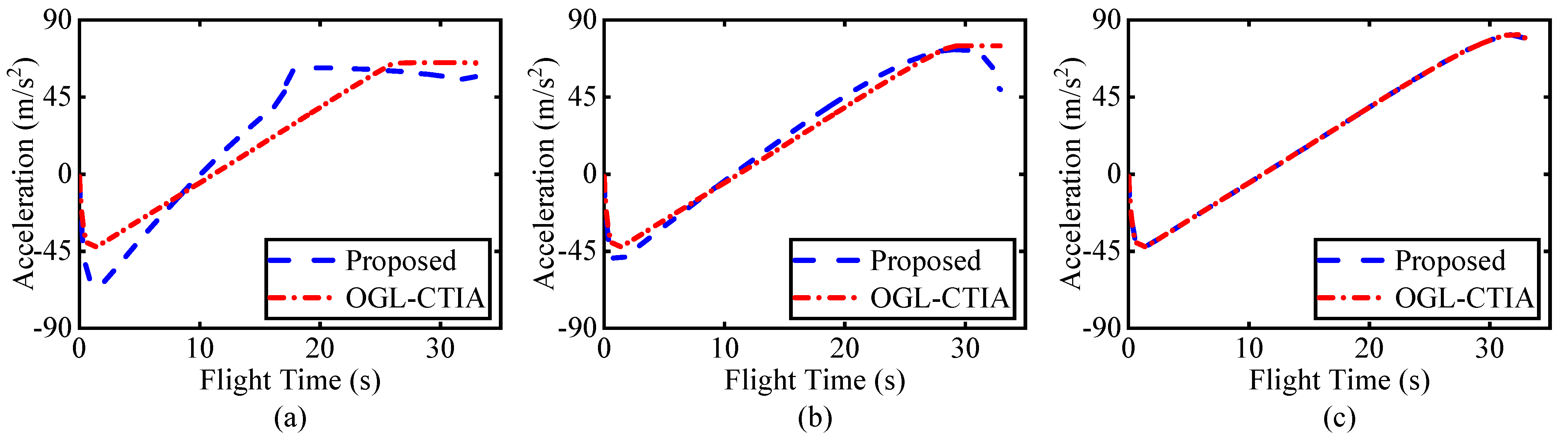
5.2. Comparison with Other Guidance Law

The OGL-CTIA proposed in [10] is a widely used and effective guidance law to impose a specified impact-angle. In this subsection, a comparison between the proposed guidance law and OGL-CTIA is provided to demonstrate the superior performance of the proposed guidance law in limiting maximum acceleration. In the simulations, the engagement condition is set to case 1 and the various acceleration limits are involved.

Figure 12 shows the interception trajectories of both guidance laws with $u_{\lim }=65,75,85 \mathrm{m}/{\mathrm{s}}^2$. As can be seen from those figures, both guidance laws perform well when the acceleration limit is $85 \mathrm{m}/{\mathrm{s}}^2$. If the acceleration limit is stricter to $65 \mathrm{m}/{\mathrm{s}}^2$ or $75 \mathrm{m}/{\mathrm{s}}^2$, the proposed method also performs well. However, the OGL-CTIA fails to intercept the target. The statistics of the miss distances and the impact-angle errors are listed in

Table 2. Miss Distances and Impact-angle Errors of Two Guidance Laws.

Acceleration Limit (m/s2)	Proposed Guidance		OGL-CTIA
	Miss (m)	Angle Error (deg)	Miss (m)	Angle Error (deg)
65	2.04 × 10-3	1.52 × 10-3	257.54	1.26
75	7.42×10-3	8.08×10-3	32.88	0.26
85	3.68 × 10-3	4.11 × 10-3	3.68 × 10-3	4.11 × 10-3

. The computational time at every guidance step of the proposed method and OGL-CTIA is presented in Figure 13. It is obvious that the computational time of the proposed method is almost same as that of OGL-CTIA. Therefore, the increase of computational burden due to solving the optimal weighted gain is less and negligible, so the real-time computational feasibility of the proposed method can be guaranteed.

The missile’s accelerations for different guidance laws are given in Figure 14. It is obvious that the accelerations of all cases for the proposed guidance law are within the limiting value throughout the homing phase. However, the acceleration for OGL-CTIA saturates during the last seconds when the acceleration limits are restricted to $75\mathrm{m}/{\mathrm{s}}^2$ and $65\mathrm{m}/{\mathrm{s}}^2$. That leads to the failure to intercept the target. It should be noted that only one case is successful because the acceleration limiting value is only $85\mathrm{m}/{\mathrm{s}}^2$, which is much looser than that in other cases. Conclusively, the proposed guidance law improves the effectiveness of direct hit in comparison with other guidance laws. Note that a saltation in the acceleration profile of the proposed guidance law occurred for the case with $u_{\lim }=65\mathrm{m}/{\mathrm{s}}^2$. The reason is that, at this point, $N$ suddenly becomes zero in response to the coming acceleration saturation, which is shown in Figure 15.

The miss distance, impact-angle error, and the total maneuvering energy for different acceleration limiting values are displayed in Figure 16. Obviously, the proposed guidance law can achieve successful interception with desired impact-angle if the acceleration limiting value is as low as 62 m/s². However, OGL-CTIA will fail if the acceleration limit is below 82 m/s². This is because the acceleration saturates during the last seconds when the acceleration limits are stricter, causing large miss distance and terminal angle error. Although the total maneuvering energy has increased, it is not too much, by only 11.5%. Therefore, it is easy to conclude that the proposed guidance law has a superior performance in dealing with the stricter acceleration limit in comparison with typical OGL-CTIA.

6. Conclusions

A guidance law is proposed for imposing a predetermined impact-angle with the acceleration limit using linear optimal control methodology. This guidance law introduces a time-varying weighted function at the cost of control energy so that the acceleration profile can be regulated by adjusting the weighted gain. Furthermore, the relationship between the maximum of guidance command, the total maneuvering energy and the weighted gain is derived in the framework of linear lag-free system. And a method to select the suitable weighted gain to limit the maximum acceleration is developed. Several numerical simulations with linear lag-free system, nonlinear lag-free system, and nonlinear lag system are carried out to verify the performance of the proposed guidance law. The results demonstrate that, even when the scenario is initiated with largely different impact-angle requirement, the guidance laws exhibited excellent performance by providing near-zero miss distance and intercept angle error. Additionally, the proposed guidance law also has superior performance in dealing with the stricter acceleration limit in comparison with typical OGL-CTIA. Benefiting from this character, the proposed method greatly improves the interceptor’s warhead lethality, resulting in possible warhead size reduction.

References

1. Han, T.; Hu, Q.; Xin, M. Analytical solution of field-of-view limited guidance with constrained impact and capturability analysis. Aerosp. Sci. Technol. 2020, 97, 105586. [Google Scholar] [CrossRef]
2. Liu, B.; Hou, M.; Feng, D. Nonlinear mapping based impact angle control guidance with seeker’s field-of-view constraint. Aerosp. Sci. Technol. 2019, 86, 724–736. [Google Scholar] [CrossRef]
3. Bryson, A.E.; Ho, Y.-C. Applied Optimal Control; John Wiley & Sons: New York, NY, USA, 1975; pp. 154–155. [Google Scholar]
4. Ben-Asher, J.Z.; Yaesh, I. Advances in Missile Guidance Theory; AIAA, Inc.: Reston, VA, USA, 1998; pp. 123–130. [Google Scholar]
5. Kim, M.; Grider, K.V. Terminal Guidance for Impact Attitude Angle Constrained Flight Trajectories. IEEE Trans. Aerosp. Electron. Syst. 1973, AES-9, 852–859. [Google Scholar] [CrossRef]
6. York, R.J.; Pastrick, H.L. Optimal Terminal Guidance with Constraints at Final Time. J. Spacecr. Rocket. 1977, 14, 381–383. [Google Scholar] [CrossRef]
7. Pastrick, H.; York, R. Optimal control for an air defense interceptor: Part I. In Proceedings of the 1980 IEEE Southeastcon, Knoxville, TN, USA, 10–13 April 1980; pp. 229–232. [Google Scholar]
8. Ryoo, C.-K.; Cho, H.; Tahk, M.-J. Optimal Guidance Laws with Terminal Impact Angle Constraint. J. Guid. Control Dyn. 2005, 28, 724–732. [Google Scholar] [CrossRef]
9. Song, T.L.; Shin, S.J.; Cho, H. Impact Angle Control for Planar Engagements. IEEE Trans. Aerosp. Electron. Syst. 1999, 35, 1439–1444. [Google Scholar] [CrossRef]
10. Shaferman, V.; Shima, T. Linear Quadratic Guidance Laws for Imposing a Terminal Intercept Angle. J. Guid. Control Dyn. 2008, 31, 1400–1412. [Google Scholar] [CrossRef]
11. Rusnak, I.; Weiss, H.; Eliav, R. Missile guidance with constrained terminal body angle. In Proceedings of the 2010 IEEE 26th Convention of Electrical and Electronics Engineers in Israel, Eilat, Israel, 17–20 November 2010; pp. 45–49. [Google Scholar]
12. Idan, M.; Golan, O.M.; Guelman, M. Optimal planar interception with terminal constraints. J. Guid. Control Dyn. 1995, 18, 1273–1279. [Google Scholar] [CrossRef]
13. Chang-Kyung, R.; Hangju, C.; Min-Jea, T. Time-to-go weighted optimal guidance with impact angle constraints. IEEE Trans. Control Syst. Technol. 2006, 14, 483–492. [Google Scholar] [CrossRef]
14. Ohlmeyer, E.J. Control of terminal engagement geometry using generalized vector explicit guidance. In Proceedings of the 2003 American Control Conference, Denver, CO, USA, 4–6 June 2003; pp. 396–401. [Google Scholar]
15. Ohlmeyer, E.J.; Phillips, C.A. Generalized Vector Explicit Guidance. J. Guid. Control Dyn. 2006, 29, 261–268. [Google Scholar] [CrossRef]
16. He, S.; Lee, C.-H. Optimal Impact Angle Guidance for Exoatmospheric Interception Utilizing Gravitational Effect. IEEE Trans. Aerosp. Electron. Syst. 2019, 55, 1–10. [Google Scholar] [CrossRef] [Green Version]
17. Lee, C.-H.; Tahk, M.-J.; Lee, J.-I. Generalized Formulation of Weighted Optimal Guidance Laws with Impact Angle Constraint. IEEE Trans. Aerosp. Electron. Syst. 2013, 49, 1317–1322. [Google Scholar] [CrossRef] [Green Version]
18. Xiong, S.; Wei, M.; Zhao, M.; Xiong, H.; Wang, W.; Zhou, B. Hyperbolic tangent function weighted optimal intercept angle guidance law. Aerosp. Sci. Technol. 2018, 78, 604–619. [Google Scholar] [CrossRef]
19. Li, C.; Wang, J.; He, S.; Lee, C.-H. Collision-geometry-based generalized optimal impact angle guidance for various missile and target motions. Aerosp. Sci. Technol. 2020, 106, 106204. [Google Scholar] [CrossRef]
20. Kim, B.S.; Lee, J.G.; Han, H.S. Biased PNG law for impact with angular constraint. IEEE Trans. Aerosp. Electron. Syst. 1998, 34, 277–288. [Google Scholar] [CrossRef]
21. Ratnoo, A.; Ghose, D. Impact Angle Constrained Guidance Against Nonstationary Nonmaneuvering Targets. J. Guid. Control Dyn. 2010, 33, 269–275. [Google Scholar] [CrossRef]
22. Erer, K.S.; Merttopçuoglu, O. Indirect Impact-Angle-Control Against Stationary Targets Using Biased Pure Proportional Navigation. J. Guid. Control Dyn. 2012, 35, 700–704. [Google Scholar] [CrossRef]
23. Kim, T.-H.; Park, B.-G.; Tahk, M.-J. Bias-Shaping Method for Biased Proportional Navigation with Terminal-Angle Constraint. J. Guid. Control Dyn. 2013, 36, 1810–1816. [Google Scholar] [CrossRef]
24. Lee, C.-H.; Kim, T.-H.; Tahk, M.-J. Interception Angle Control Guidance Using Proportional Navigation with Error Feedback. J. Guid. Control Dyn. 2013, 36, 1556–1561. [Google Scholar] [CrossRef]
25. Kumar, S.R.; Rao, S.; Ghose, D. Sliding-Mode Guidance and Control for All-Aspect Interceptors with Terminal Angle Constraints. J. Guid. Control Dyn. 2012, 35, 1230–1246. [Google Scholar] [CrossRef]
26. Cho, D.; Kim, H.J.; Tahk, M.-J. Impact angle constrained sliding mode guidance against maneuvering target with unknown acceleration. IEEE Trans. Aerosp. Electron. Syst. 2015, 51, 1310–1323. [Google Scholar] [CrossRef]
27. Ji, Y.; Lin, D.; Wang, W.; Hu, S.; Pei, P. Three-dimensional terminal angle constrained robust guidance law with autopilot lag consideration. Aerosp. Sci. Technol. 2019, 86, 160–176. [Google Scholar] [CrossRef]
28. Chen, Z.; Chen, W.; Liu, X.; Cheng, J. Three-dimensional fixed-time robust cooperative guidance law for simultaneous attack with impact angle constraint. Aerosp. Sci. Technol. 2021, 110, 106523. [Google Scholar] [CrossRef]
29. Hu, Q.; Cao, R.; Han, T.; Xin, M. Field-of-view limited guidance with impact angle constraint and feasibility analysis. Aerosp. Sci. Technol. 2021, 114, 106753. [Google Scholar] [CrossRef]
30. Rusnak, I.; Meir, L. Optimal guidance for acceleration constrained missile and maneuvering target. IEEE Trans. Aerosp. Electron. Syst. 1990, 26, 618–624. [Google Scholar] [CrossRef]
31. Hexner, G.; Shima, T.; Weiss, H. LQG Guidance Law with Bounded Acceleration Command. IEEE Trans. Aerosp. Electron. Syst. 2008, 44, 77–86. [Google Scholar] [CrossRef]
32. Weiss, M.; Shima, T. Optimal Linear-Quadratic Missile Guidance Laws with Penalty on Command Variability. J. Guid. Control Dyn. 2015, 38, 226–237. [Google Scholar] [CrossRef]
Figure 1. The Planar engagement geometry.
Aerospace 08 00358 g001
Figure 2. The value of C ¯ 2 for the various κ 0 . (a) κ 0 , 1 , N add = 0 , + , N sub = ; (b) κ 0 1 , 2 / 3 , N add = 0 , N 1 N 3 , + , N sub = N 2 , N 3 ; (c) κ 0 2 / 3 , 1 / 3 , N add = N 3 , + , N sub = max 0 , N 2 , N 3 ; (d) κ 0 1 / 3 , + , N add = 0 , + , N sub = .
Aerospace 08 00358 g002
Figure 3. u ¯ M a x 0 and u ¯ M a x N e x t u 1 for various κ 0 .
Aerospace 08 00358 g003
Figure 4. N e x t u 1 and N z e r o a d d for various κ 0 .
Aerospace 08 00358 g004
Figure 5. The trajectory of Θ a N , κ 0 = 0 .
Aerospace 08 00358 g005
Figure 6. The flowchart of implementation.
Aerospace 08 00358 g006
Figure 7. ZEM and ZEAE. (a) case 1; (b) case 2; (c) case 3.
Aerospace 08 00358 g007
Figure 8. Missile acceleration. (a) case 1; (b) case 2; (c) case 3.
Aerospace 08 00358 g008
Figure 9. Some comparisons for three systems in case 1. (a) Maximum acceleration; (b) Dimensionless time-to-go corresponding to the maximum acceleration; (c) History of the missile acceleration.
Aerospace 08 00358 g009
Figure 10. Some comparisons for three systems in case 2. (a) Maximum acceleration; (b) Dimensionless time-to-go corresponding to the maximum acceleration; (c) History of the missile acceleration.
Aerospace 08 00358 g010
Figure 11. Some comparisons for three systems in case 3. (a) Maximum acceleration; (b) Dimensionless time-to-go corresponding to the maximum acceleration; (c) History of the missile acceleration.
Aerospace 08 00358 g011
Figure 12. Interception trajectories. (a) u lim = 65   m / s 2 ; (b) u lim = 75   m / s 2 ; (c) u lim = 85   m / s 2 .
Aerospace 08 00358 g012
Figure 13. Computational time. (a) u lim = 65   m / s 2 ; (b) u lim = 75   m / s 2 ; (c) u lim = 85   m / s 2 .
Aerospace 08 00358 g013
Figure 14. Missile acceleration. (a) u lim = 65 m / s 2 ; (b) u lim = 75 m / s 2 ; (c) u lim = 85 m / s 2 .
Aerospace 08 00358 g014
Figure 15. κ and N with u lim = 65   m / s 2 .
Aerospace 08 00358 g015
Figure 16. Interception results for various acceleration limiting values. (a) Miss distance; (b) Impact-angle error; (c) Total maneuvering energy.
Aerospace 08 00358 g016