A Multi-Objective Coverage Path Planning Algorithm for UAVs to Cover Spatially Distributed Regions in Urban Environments

Abstract

This paper presents a multi-objective coverage flight path planning algorithm that finds minimum length, collision-free, and flyable paths for unmanned aerial vehicles (UAV) in three-dimensional (3D) urban environments inhabiting multiple obstacles for covering spatially distributed regions. In many practical applications, UAVs are often required to fully cover multiple spatially distributed regions located in the 3D urban environments while avoiding obstacles. This problem is relatively complex since it requires the optimization of both inter (e.g., traveling from one region/city to another) and intra-regional (e.g., within a region/city) paths. To solve this complex problem, we find the traversal order of each area of interest (AOI) in the form of a coarse tour (i.e., graph) with the help of an ant colony optimization (ACO) algorithm by formulating it as a traveling salesman problem (TSP) from the center of each AOI, which is subsequently optimized. The intra-regional path finding problem is solved with the integration of fitting sensors’ footprints sweeps (SFS) and sparse waypoint graphs (SWG) in the AOI. To find a path that covers all accessible points of an AOI, we fit fewer, longest, and smooth SFSs in such a way that most parts of an AOI can be covered with fewer sweeps. Furthermore, the low-cost traversal order of each SFS is computed, and SWG is constructed by connecting the SFSs while respecting the global and local constraints. It finds a global solution (i.e., inter + intra-regional path) without sacrificing the guarantees on computing time, number of turning maneuvers, perfect coverage, path overlapping, and path length. The results obtained from various representative scenarios show that proposed algorithm is able to compute low-cost coverage paths for UAV navigation in urban environments.

1. Introduction

Unmanned aerial vehicles (UAVs) are playing a vital role in the realization of smart cities, smart building, and smart infrastructures with innovative applications. Due to the rapid developments in the low-cost control methods and the wide range of sensors, UAV applications in urban areas have significantly increased [1]. UAVs can contribute to improving the quality of people’s lives. The technological developments such as low-powered hardware, embedded software, reactive controls, long-range wireless communication, onboard computation, and other such technologies have enabled UAVs to perform complex missions autonomously. The recent technological developments have significantly enhanced the UAV endurance, localization, motion accuracy, self-awareness, and the level of autonomy in the airspace. The use of UAVs is rapidly increasing in many sectors, especially in urban areas due to their sensing and avoidance (SAA) abilities which allow them to navigate safely in airspace [2]. UAVs are capable of performing various missions in an economical and convenient way compared to traditional human-based approaches. According to the Teal Group Corporation forecasts, the annual spending on UAVs will be more than USD 12 billion in the coming five years [3]. Furthermore, with the integration of internet of things and cloud computing technologies, UAVs have become a powerful tool for data collection [4].

The real-life practical applications of UAVs such as communication relays [5], building construction monitoring [6], searching for rescue victims [7], inspection of aging infrastructure [8], goods delivery [9], air quality monitoring [10], disaster management [11], remote sensing [12], soybean yield prediction [13], visual tracking [14], content delivery [15], among others, are the most attractive applications. Besides many real-world applications in each sector, UAV usage without human onboard control imposes several challenges such as the co-ordination among UAV and the ground control station (GCS) as this can be affected by the high distances, limited onboard processing capability, weather conditions, and energy constraints etc. Moreover, collision avoidance with not only with obstacles, especially with other drones and, eventually, helicopters in complex 3D urban environments and payload constraints are noticeable challenge. Beside these challenges, in many practical applications, a UAV needs an ability to find a collision-free path between two pre-decided locations which is referred as path planning (PP) or to find a viable path which covers every reachable point of a certain area of interest (AOI) which is called coverage path planning (CPP). In this paper, we focus on the CPP problem for a UAV to cover multiple obstacle surrounded strewn AOIs located in 3D urban environments which has not been solved by prior studies.

The CPP problem is regarded as the subtopic of the PP where it is necessary to obtain a viable path that covers an entire free space of a certain AOI with a minimal cost [16]. The coverage path cost can be number of turns, computing time, path length, overlapping, energy, and smoothness. Every CPP algorithm optimizes one/more cost functions. Due to the extensive use of the UAVs in recent times, the CPP problem for single and multiple UAVs has become an active area of research [17,18]. The CPP are divided into two major categories, global and local CPP based on the information available about workspace. In global CPP, the path planning is carried out in a fully known environment (i.e., obstacles’ geometries are known). In contrast, local CPP, also known as sensor-based coverage, is relatively complex because the UAV workspace is mostly unknown [19]. The UAV employs on-board sensors to acquire workspace data to perform the coverage mission in real-time. Considering the nature of the problem, single/multiple UAVs can be deployed to perform the mission. However, deploying multiple UAVs can lead to communication and co-ordination issues among UAVs.

Many CPP methods have been reported in the literature for covering a regularly (i.e., rectangle, convex polygon) or irregularly (non-convex polygons) shaped AOI with the visual/thermal sensors mounted on a UAV [20,21]. The basic methodology used by most of these algorithms is as follows: (i) AOI decomposition into non-overlapping sub-regions, (ii) finding of the visiting order/sequence of the sub-regions, and (iii) covering decomposed sub-regions individually in a back and forth (BF) or spiral manner to obtain a coverage path. The AOI’s decomposition-based methods are promising in achieving perfect coverage of an AOI. Classical exact cellular decomposition [22], landmark-based topological coverage [23], Morse-based decomposition [24], contact sensor-based coverage [25], grid-based decomposition methods [26], and graph-based methods [27] are well-known decomposition approaches. There are works in the literature dealing with the CPP problem using simple geometric flight patterns without decomposing the AOI [28]. Meanwhile, the target area in such works is of regular shape with less complexity.

The existing CPP algorithms for UAVs do not provide thorough insight into the coverage of multiple AOIs in complex 3D urban environments with obstacles. They do not use sensor footprints (SF) as a coverage unit while decomposing the AOI, thereby causing significant path length degradation and overlapping. Li et al. [29] have explained that most of the prior CPP algorithms employ the same sweep direction in all sub-regions which may hinder finding an optimal path. The cost for switching between sub-regions is also very high. To lower path computing cost, various latest approaches such as viewpoints sampling [30], mirror mapping [31], optimal polygon decomposition [32], in-field obstacles classification [33], and context-aware UAV mobility [34] have been developed. Despite the practical nature of these approaches, in most cases, either computing time is very high, or many locations of the AOI are covered repeatedly [35]. Most of the CPP algorithms are very sensitive to the shape of the AOI [36]. When the shape of the AOI is changed, the algorithm performance is no longer acceptable. The AOI decomposition is not conducted in relation to the SFs which can increase the number of turns in the path. To overcome the above limitations, this study proposes a new CPP algorithm that fulfills the multiple objectives of the CPP with fewer SF sweeps and a sparse waypoint graph (SWG).

The rest of the paper is organized as follows. Section 2 explains the background and related work regarding well-known CPP algorithms proposed for singular and multiple AOI coverage, respectively. Section 3 presents the proposed multi-objective coverage flight path planning algorithm and explains its principal steps. Section 4 discusses the experimental results that were obtained with extensive experiments. Finally, conclusions, limitations, and promising future directions are given in Section 5.

2. Background and Related Work on CPP

This section presents the background and related work about the single AOI and multiple spatially distributed AOI coverage. Cao et al. [37] defined the six mandatory requirements for the CPP which are: (i) the UAV must move through all accessible points in AOI to ensure perfect coverage; (ii) the UAV must cover the AOI without overlapping paths; (iii) continuous and sequential operations without any repetition of paths are needed; (iv) the UAV must bypass all obstacles safely; (v) simple motion plans (e.g., straight lines or circles) should be used; and (vi) a low-cost path under available conditions is desired.

2.1. Single Area of Interest Coverage

In single AOI coverage, only one target area is covered with the assistance of single/multiple UAVs. This area can be of any geometry, and it can be located in an urban/non-urban environment. The CPP problem for the single AOI coverage has been extensively studied in the past. The detailed background about the types of AOI, decomposition techniques, geometric flight patterns, coverage types, path optimization algorithms, and well-known CPP methods are explained in Section 2.1.1, Section 2.1.2, Section 2.1.3, Section 2.1.4, Section 2.1.5 and Section 2.1.6.

2.1.1. Different Types of the Area of Interest Used for the Coverage Missions

The type of the AOI to be covered with the UAV’s sensor/camera can be 3D cubes (i.e., buildings), a rectangle/square, convex and concave polygon or of irregular shape. The shape of the AOI is an important factor, and it must be considered in the CPP process. The CPP algorithms devised for the convex-polygonal-shaped AOI cannot yield feasible results in an irregular-shaped AOI. The five most widely used AOI types are shown in Figure 1.

2.1.2. Area of Interest Decomposition Techniques Used in the Coverage Path Planning

The existing CPP methods can be classified into two major categories: cell decomposition and heuristic-based CPP methods. In the former methods, the AOI is decomposed into non-overlapping cells of varying shapes and sizes. There exist several kinds of AOI decomposition techniques [38]. The two most recognized cell-decomposition techniques are: trapezoidal decomposition [39] and boustrophedon decomposition [40]. Trapezoidal decomposition divides the AOI into convex trapezoidal cells, performs BF motions, and uses an exhaustive walk to determine the cells’ exploration sequence to perform coverage. In contrast, the boustrophedon decomposition creates non-convex larger cells considering only obstacle-vertices. The boustrophedon decomposition is superior than the trapezoidal decomposition in terms of number of cells and path length. The Morse-based cellular decomposition is an advance form of the boustrophedon decomposition, which is based on the critical points of the Morse functions [41]. Grid-based decomposition methods are also used to generate coverage paths for UAVs from grids [42]. Convex decomposition transforms the irregularly shaped AOI into the regular shaped cells to reduce the number of turns [43]. In some cases, the concave and convex decomposition both have been jointly used in the CPP problems. Each decomposition method varies regarding the cell shapes, cell sizes, degree of complexity, objectives of CPP, and path quality. For instance, the trapezoidal decomposition has overall time estimation of $O\left(n^3\right)$ which makes it unsuitable for complex problems. On the other hand, the heuristic-based methods define procedures that should be followed during the CPP process [44,45]. These methods determine a path without decomposing the AOI, and have lower computing complexities than decomposition-based methods. A pictorial overview of the six most widely used AOI decomposition techniques is depicted in Figure 2. The selection of the decomposition technique depends upon the AOI shape, application’s requirement, coverage type, flight pattern, and objectives of the CPP.

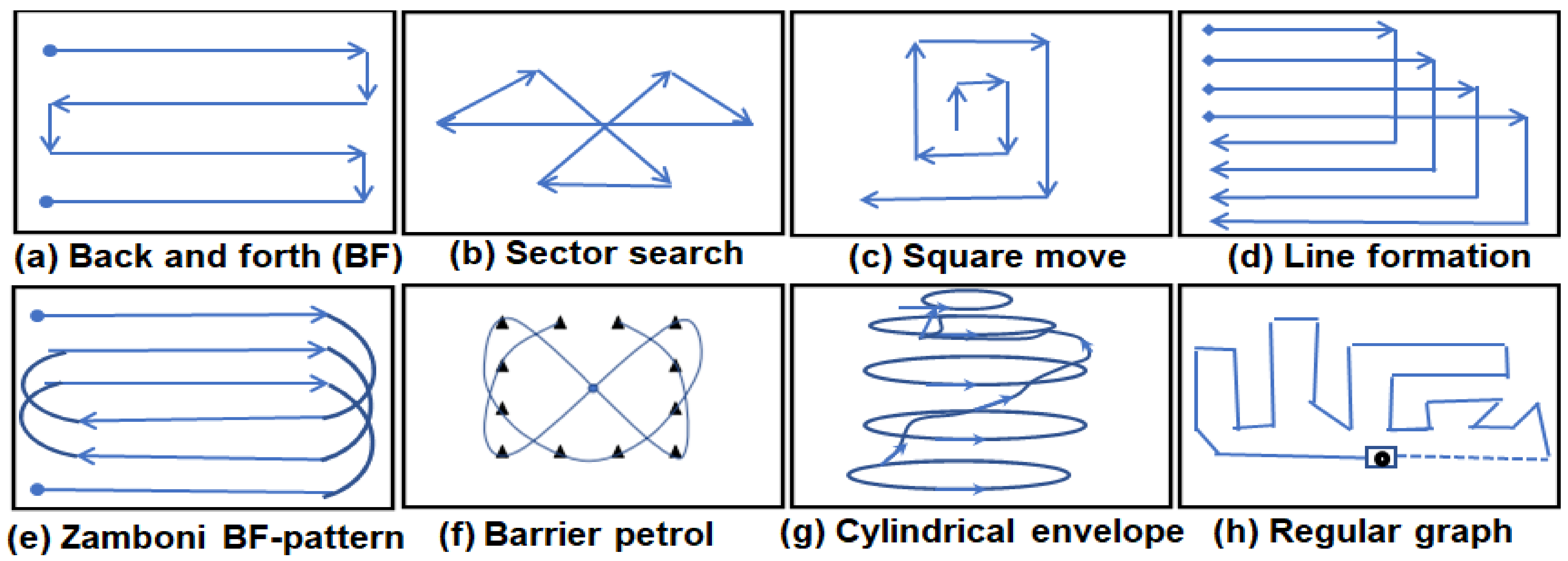
2.1.3. Geometric Flight Patterns Used in the Area of Interest Coverage

There are eight commonly used geometric flight patterns for the CPP. Andersen et al. [46] compared various types of the geometric flight patterns used for the CPP problems. The flight patterns are chosen based on the shape of the AOI, UAV mobility constraints, application requirements, and coverage type. For example, the BF pattern is suitable when the AOI is large in size and is in a rectangular shape. In Figure 3, eight well-known geometric flight patterns are presented graphically.

2.1.4. Coverage Types Employed in the Practical Scenarios with Unmanned Aerial Vehicle

Generally, there are two well-known types of the coverage for the practical scenarios. Both coverage types with examples are explained below.

• Simple coverage: In this type of coverage, the AOI is covered only once. The example of this type of the coverage are imagery, sprays, surveillance, and scans etc.
• Continuous coverage: In this type of coverage, the AOI is covered multiple times. The example of this type of coverage is objects/events detection in the AOI, and periodic readings collection from different parts of the AOI.

2.1.5. Overview of Path Optimization Algorithms Used in the Coverage Path Planning

After AOI decomposition and graph modeling from each sub region, an optimization algorithm is employed to find a coverage path. The existing studies used several types of path optimization algorithms for CPP. The most promising optimization algorithms are the genetic algorithm [47], the ACO algorithm [48], the A* algorithm [49], particle swarm optimization [50], the theta* algorithm [51], the wavefront algorithm [52], and their improved versions. Furthermore, in some cases, two different optimization algorithms can also be employed simultaneously for the inter and intra-region coverage [53]. This work uses an ACO algorithm [48] for computing the traversal order of AOI and sweeps, respectively.

2.1.6. State-of-the-Art Coverage Path Planning Methods

Finding a low-cost coverage path to ensure the perfect coverage of an AOI is an attractive topic for research. Öst [54] proposed a CPP algorithm for a concave shape AOI with sharp edges without sacrificing the guarantees on the perfect coverage. It employs convex decomposition to transform the complex shape AOI into smaller regular cells. BF and SP patterns are jointly used to fully cover the given AOI. It has an ability to handle the complex shaped AOI with only marginal loss in the solution quality. Xu et al. [55] proposed an optimal CPP algorithm for a fixed wing UAV with minimum overlapping and complete coverage guarantees. It employs boustrophedon decomposition to decompose the AOI into a set of non-overlapping cells. Later, the adjacency graph is generated from the cells, and each cell is swept using the BF flight patterns. The order of the cells visit follows the Eulerian circuit concept with the start and end at the same vertex of the cell. It guarantees the complete coverage of the given AOI. However, in some cases, it may perform additional sweeps when an obstacle’s geometry is complex by not considering the SF as the coverage unit, and thereby the path length can be degraded. Jiao et al. [56] devised an exact cellular decomposition-based approach for the concave area coverage. Initially, the concave-shaped AOI is decomposed into the convex subareas using minimum width sum approach [57], and then the BF flight pattern is employed to completely sweep the AOI.

Table 1. Description of the state-of-the art coverage path planning approaches used in single AOI coverage.

Decomposition Type	Shape of the AOI	Detailed Comparison of State-of-the Art Coverage Path Planning Approaches
		Evaluation Criteria	CPP for	Approach	Agent Type	Representative Methods
No decomposition	Polygonal 3D Topology Regular Grids Rectangular Rectangular	Flight time Energy consumption Energy consumption and Mission time Coverage rate and time Flight time	Single UAV Single UAV Single UAV Multiple UAVs Multiple UAVs	Back and forth CPP Three-stage Energy-aware CPP E-MoTA e I-MoTA Dynamic programming MILP approach	Fixed wing Rotary wing Both Fixed wing Fixed wing	Coombes et al. [58] Li et al. [59] Artemenko et al. [60] Ahmadzadeh et al. [61] Forsmo et al. [62]
Exact cellular decomposition	Polygonal Irregular Polygonal Irregular Rectangular	Number of turns and path length Path length and coverage time Number of turning maneuvers Interval of visits and information latency Target detection and search time	Single UAV Single UAV Single UAV Multiple UAVs Multiple UAVs	Back-and-Forth CPP Back-and-Forth CPP Back-and-Forth CPP One-to-one coordination Line Formation-based CPP	Rotary wing Fixed wing Both Both Rotary wing	Torres et al. [63] Xu et al. [64] Li et al. [29] Acevedo et al. [65] Vincent et al. [66]
Approximate cellular decomposition	Irregular/Regular Grid Regular Grid Square Square Polygonal Rectangular Regular Grid 3D cube (building)	Coverage time Path length Total distance of the coverage Total distance of the coverage Path length Mission completion time Coverage rate and coverage ratio Computing time	Single UAV Single UAV Single UAV Single UAV Single UAV Multiple UAVs Multiple UAVs Single UAV	Gradient-based CPP Simulated annealing Hilbert space-filling curves BFS, DFS, and SH Genetic Algorithm Multi-Objective CPP with GA Chaotic ACO algorithm TOGVF transition	Rotary wing Rotary wing Rotary wing Rotary wing Rotary wing Rotary wing Rotary wing Both	Valente et al. [67] Xiao et al. [68] Sadat et al. [69] Sadat et al. [70] Trujillo et al. [71] Hayat et al. [72] Rosalie et al. [73] Yao et al. [17]

summarizes state-of-the-art CPP methods.

The CPP algorithms devised to solve the AOI coverage problem are mostly concerned with the planning phase to find a complete path while optimizing certain performance metrics. However, a considerable attention is required when planning a coverage path for the fixed-wing UAVs, as these UAVs cannot make the abrupt directional changes. Hence, the CPP algorithm must also consider the motion constraints of such UAVs during the pathfinding process [36,74]. Some studies devised application-specific methods such as CPP for interesting and non-interesting zones [69,70]. The interesting zones need careful observation at higher resolution, so the UAV scans such area/zones with relatively lower altitudes. In contrast, the non-interesting zones are covered from higher altitudes with decreased resolutions to reduce the overall path cost.

2.2. Spatially Distributed and Multiple AOI Coverage

In many practical applications, the UAV needs the ability to cover multiple spatially distributed regions located in urban environments. For example, when a disaster occurs, multiple spatially distributed regions may need damage assessment, and the UAV is a low-cost tool for this purpose. Furthermore, in search and rescue (SAR) missions, spatially distributed region coverage is often required to find the targets or to collect data. The CPP for covering spatially distributed regions is also needed in many other applications such as room cleaning, lawn mowing, and infrastructure inspection. Bouzid et al. [75] proposed an optimal CPP approach for the several points of interest (POIs) for coverage with a quad rotor UAV. Their approach consists of two steps; firstly, the cost to visit the adjacent POI is calculated, and then the sequence of POIs visit is determined aiming to reduce the global path length. They formulated the POI visits problem as TSP, and solved it with a genetic algorithm. The proposed approach can generate the closed path of shortest length while visiting each POI only once. A few studies focused on the CPP to cover spatially distributed regions. Xie et al. [76] proposed an optimal CPP algorithm for UAVs to cover multiple regions. The approach makes use of advanced dynamic programming to solve the integrated problem of TSP and CPP. Jincheng et al. [77] proposed an online CPP algorithm for multi-region surveillance with no more than one turn while covering several AOIs. It performs better than the zig-zag path planner. Huang et al. [78] presented a comprehensive study regarding several typical problems in designing an internet of flying robots (IoFR) for practical applications. They classified the coverage into three types: camera coverage, charging coverage, and communication coverage, and discussed the CPP for each category. Vasquez et al. [79] proposed an algorithm for surveying the disjoint areas with UAVs. Xie et al. [80] devised a generic method for covering multiple spatially distributed regions. However, these approaches are not suitable for use in urban environments inhabited by multiple obstacles.

2.3. Major Contributions in the Field of UAV CPP for Spatially Distributed Regions Coverage

The major contributions of this research are summarized as follows: (i) it proposes a new multi-objective CPP algorithm that has the potential to obtain a flyable path that ensures the perfect coverage of the multiple spatially distributed regions located in urban environments, with reduced path length, coverage time, turning maneuvers, and path overlapping, something that previously proposed CPP algorithms based on the similar principles could not do; (ii) it finds a low-cost traversal order for the multiple areas’ visits in the form of a directed graph that is optimized afterwards based on environment complexity; (iii) it introduces a new sensor’s footprints sweeps (SFSs) fitting method by exploiting the obstacle geometry information in such a way that all the free spaces of an AOI can be swept with as few SFSs as possible; (iv) it constructs a sparse waypoint graph (SWG) by joining the footprint sweeps’ endpoints with their neighbors’ sweeps by taking into account the optimization objectives and global and local constraints; (v) it proposes a lightweight mechanism to switch between regions while avoiding collision with obstacles; (vi) to the best of our knowledge, this is the first work that solves the spatially distributed region coverage problem in urban environments with obstacles.

3. The Proposed Multi-Objective Coverage Flight Path Planning Algorithm

The SFS fitting and a SWG-based CPP algorithm is proposed to resolve the time performance, number of turns, path length, and path overlapping issues stemming from the computationally expensive decomposition techniques used for the coverage missions in obstacle-rich urban environments. The proposed algorithm not only ensures the complete coverage of a single AOI; it also computes the shortest length path between spatially distributed AOI to allow the UAV to cover multiple AOIs successfully without sacrificing guarantees on the target objectives. It computes a coverage path with reduced cost, and it enables the UAV to sweep all target areas fully in one round. This section explains the conceptual overview of the proposed multi-objective CPP algorithm and outlines its key steps. Figure 4 presents the conceptual overview of the proposed algorithm.

To find a coverage path $\mathsf{\Gamma }$ that covers an entire free space of a multiple AOI, $\{Q_1,Q_2,Q_3,\cdots ,Q_n\}$ located in a 3D urban environment of completely known geometry, we used the seven key steps, (i) modeling of the UAV operating environment from a raw urban environment map; (ii) locating AOIs on a modeled map; (iii) computing the low-cost traversal order of the AOI visits in a directed graph form; (iv) finding intra-regional path from an AOI based on the UAV initial location, using six key steps described in Section 3.4.1, Section 3.4.2, Section 3.4.3, Section 3.4.4, Section 3.4.5 and Section 3.4.6; (v) determining the next AOI to switch from the current AOI with low-cost; (vi) switching to the next AOI by formulating and solving it as a PP problem; and (vii) repeating the intra-inter regional pathfinding process until the completion of last AOI (i.e., $Q_n$). Brief discussion about each key step with formalization is below.

3.1. Modeling of the UAV’s Operating Environment from a Real Urban Environment Map

After obtaining the required information related to the coverage mission, the proposed CPP algorithm models and the UAV operating environment (i.e., workspace). Generally, it refers to the classification of the free spaces $\left(Q_{free}\right)$, and obstacle regions $\left(Q_{obstacles}\right)$. The $Q_{obstacles}$ refers to the non-traversal parts of the AOI Q because the UAV cannot fly in these parts due to the presence of obstacles. In contrast, $Q_{free}$ refers to those parts of the Q where UAV can operate safely and the probability of collision with obstacles is zero. The obstacles present in the operating environment are modeled with the help of geometrical shapes (i.e., cubes, squares, and circles, etc.). In this paper, UAV’s operating environment from a raw urban environment map containing the elevation data about the apartments, trees, and buildings, etc. was modeled with a set of 3D convex obstacles. This is done by calculating the convex hull of the elevation data. Each modeled obstacle has random geometry (i.e., width, length and height) depending upon the real object geometry present in an urban environment. Each convex obstacle has six faces and eight vertices. The obstacle vertices v in the modeled map can be represented with three co-ordinates values, $v=(x,y,z)$. An ith obstacle vertex along with their numerical values can be mathematically expressed as the matrix given below.

$$O_i=\left[\begin{array}{ccccc}{x}_{min}& y_{min}& z_{max};x_{min}& y_{min}& z_{min}\\ x_{min}& y_{max}& z_{max};x_{min}& y_{max}& z_{min}\\ x_{max}& y_{min}& z_{max};x_{max}& y_{min}& z_{min}\\ x_{max}& y_{max}& z_{max};x_{max}& y_{max}& z_{min}\end{array}\right]=\left[\begin{array}{ccccc}573& 919& 245;573& 919& 0\\ 573& 1038& 245;573& 1038& 0\\ 653& 919& 245;653& 919& 0\\ 653& 1038& 245;653& 1038& 0\end{array}\right]$$

where $min$ and $max$ refer to minimum and maximum values of the respective axis, respectively. The UAV source (i.e., depot) and mission completion locations are represented with 3D points $v_s$ and $v_c$, respectively. In some studies, $v_s$ and $v_c$ are the same as the UAV returns to the initial location after completing the whole mission. In this work, we consider the alternate case in which UAV does not return to the $v_s$ after finishing the mission due to the power issues. The objective of the proposed CPP algorithm is to find a coverage path $\mathsf{\Gamma }$ for a UAV mission. The path $\mathsf{\Gamma }$ consists of several nodes which have two characteristics, (i) $\mathsf{\Gamma }\in Q_{free}$ and (ii) $\mathsf{\Gamma }\cap Q_{obstacles}=\varnothing$.

3.2. Locating All Areas of Interest on a Modelled Map

The proposed CPP algorithm locates all AOIs on the 3D modelled map based on their geometry information specified in the inputs. The AOI $Q_i$ can be represented with the sequence of p vertices, $\{p_1,p_2,p_3,\cdots ,p_n\}$. Each $Q_i$ vertex $p_i$ has three co-ordinates values $(p_x\left(i\right),p_y\left(i\right),p_z\left(i\right))$, where $p_z\left(i\right)=0$. Let $p_i$ be the initial vertex of a $Q_i$; the next vertex to $p_i$ can be represented as $p_{next\left(i\right)}$, where $next\left(i\right)=i\left(modn\right)+1$. The line $e_i$ connecting two vertices $p_i$ and $p_{next\left(i\right)}$ has length $l_i$. The $Q_i$ boundary (i.e., combinations of vertices and edges) can intersect with the obstacles. The four practical cases in this regard are: (i) the $Q_i$ vertices and edges do not intersect with obstacles at all, (ii) the $Q_i$ vertices can lie within obstacles, (iii) the $Q_i$ edges intersect with obstacles, and (iv) combinations of (ii) and (iii). When the $Q_i$ boundary hits obstacles, boundary simplification is then applied in the intra-regional path computation considering the nearby obstacles. In some scenarios, the $Q_i$ can contain many no-fly zones (NFZ) of distinct geometries, and our algorithm locates those NFZs in the respective AOI at this stage.

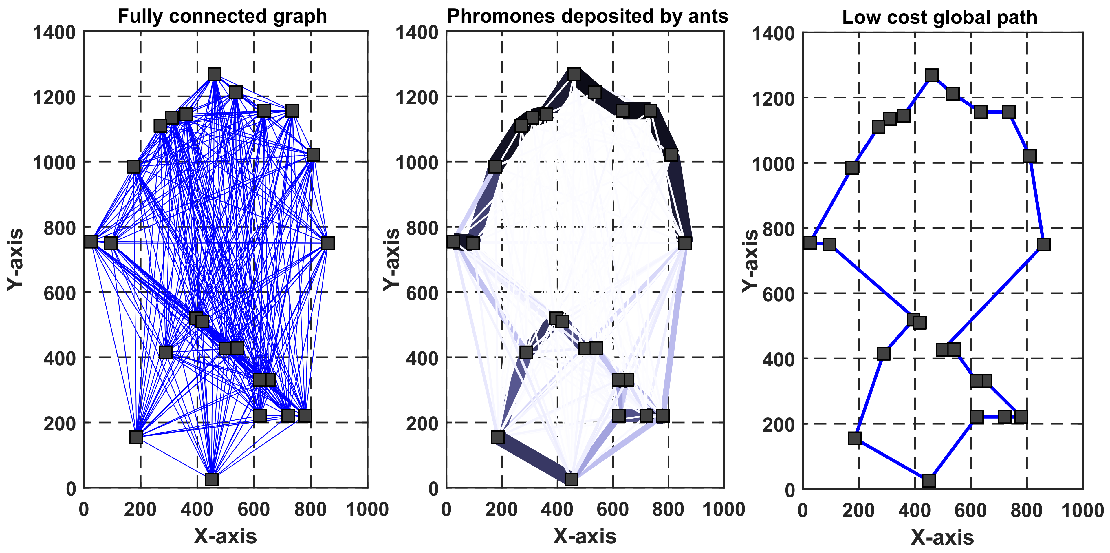
3.3. Computing Low-Cost Traversal Order of the Area of Interests in the Form of a Graph

After locating all AOIs on the modeled map as per their geometries, the next step is to compute the low-cost traversal order (e.g., process of passing across) of the AOIs for computing the global path. To do so, the centroids of each AOI were determined initially. To find the center $C_{Q_i}$ of an $ith$ AOI which is in rectangular form with four vertices ($p=4$), we applied the following procedure to find the $Q_i$ center. The four vertices values are given which are: $p_1=(800,40,0)$, $p_2=(800,1000,0)$, $p_3=(1000,40,0)$, $p_4=(1000,1000,0)$. We find the two unknown vertices $p_5$ and $p_6$ with the help of Equations (1) and (2).

$$p_5=(p_x\left(1\right),\frac{p_y\left(1\right)+p_y\left(2\right)}{2},p_z\left(1\right)).$$

(1)

$$p_6=(p_x\left(3\right),\frac{p_y\left(3\right)+p_y\left(4\right)}{2},p_z\left(3\right)).$$

(2)

In Equations (1) and (2), the x-axis and $z\text{-}\mathrm{axis}$ values were fixed. One can fix the y-axis and $z\text{-}\mathrm{axis}$ values, and can find the unknown points using x-axis values. After finding the $p_5$ and $p_6$ points values, the $C_{Q_i}$ value can be determined using (3).

$$C_{Q_i}=(\frac{p_x\left(5\right)+p_x\left(6\right)}{2},p_y\left(5\right),p_z\left(5\right)).$$

(3)

In $Q_i$, the four vertices’ geometry values are fully known, hence the $C_{Q_i}$ value is $C_{Q_i}=(900,520,0)$. With the help of a similar procedure, the centroids of each AOI are determined. Meanwhile, if the AOI’s shape is not regular, then it is converted to the regular shape (i.e., square/rectangle) first with sufficient accuracy by computing the convex-hull. Later, the midpoints are determined using the relevant axis values. The computed centroids information is stored in set $C_Q$, where $C_Q=\{C_{Q_1},C_{Q_2},C_{Q_3},\cdots ,C_{Q_N}\}$ for further processing. Once, the centroids of all AOIs are determined, we formulate the traversal order computation problem as a traveling salesman problem (TSP) (i.e., each AOI must be visited only once), and the ACO algorithm is employed to solve this TSP. Before computing the traversal order, the UAV depot location $v_s$ is added in set $C_Q$, and $C_Q=\{v_s,C_{Q_1},C_{Q_2},C_{Q_3},\cdots ,C_{Q_N}\}$, as it assists in determining the first AOI to be visited as per the UAV initial location.

Given the N-point set $C_Q$ originally determined from the AOI’s vertices, these points are used to calculate a close path that visits each AOI’s center exactly once. We specify the required parameters of an ACO algorithm such as the number of iterations ($y_{itr}$), the number of ants (ℓ), the number of points (i.e., centroids, and UAV location) (n), the parameter to regulate the influence of pheromones ($\alpha$), the parameter to regulate the influence of visibility (sight) among two centroids ($\beta$), and the pheromone evaporation rate ($\rho$), where $\rho \in [0,1]$ values are based on the set $C_Q$ size. After specifying the parameters’ values, the distance and sight matrix are computed between centroids. Then, ℓ ants are deployed on random points, and the computation process is started for the pre-specified iterations $y_{itr}$. During this process, each ant ${\ell }_i$ determines a tour $T_{{\ell }_i}$ by remembering the points (i.e., AOI’s centroids) which have already been explored, and choosing the nearby points from its current location based on the action choice rule, formalized in Equation (4). The probability p that point $C_{Q_j}$ will be visited by an ant ${\ell }_i$ which is currently at point $C_{Q_i}$ can be computed from the following equation.

$$p_{C_{Q_i}{C}_{Q_j}}^{{\ell }_i}=\left\{\begin{array}{c}{\displaystyle \frac{{\left[{\tau }_{C_{Q_i}{C}_{Q_j}}\right]}^{\alpha }[{\eta }_{C_{Q_i}{C}_{Q_j}}{]}^{\beta }}{{\displaystyle \sum _{s\in {allowed}_{{\ell }_i}}}{\left[{\tau }_{C_{Q_i}{C}_{Q_j}}\right]}^{\alpha }[{\eta }_{C_{Q_i}{C}_{Q_j}}{]}^{\beta }}},C_{Q_j}\in allowe{d}_{{\ell }_i},\hfill \\ 0,otherwise,\hfill \end{array}\right.$$

(4)

where ${\tau }_{C_{Q_i}{C}_{Q_j}}$ represents the intensity of the pheromones trial between point $C_{Q_i}$ and $C_{Q_j}$, $\alpha$ is a parameter used to regulate the influence of ${\tau }_{C_{Q_i}{C}_{Q_j}}$, the variable ${\eta }_{C_{Q_i}{C}_{Q_j}}$ represents the visibility between point $C_{Q_j}$ and $C_{Q_i}$, which is computed as $1/d_{C_{Q_i}{C}_{Q_j}}$ (where $d_{C_{Q_i}{C}_{Q_j}}$ is the Euclidean distance between two points computed from Equation (5)), $\beta$ is a parameter used to regulate the influence of ${\eta }_{C_{Q_i}{C}_{Q_j}}$, and $allowe{d}_{{\ell }_i}$ represents the points that have not been visited by an ant ${\ell }_i$ yet, respectively.

$$d_{C_{Q_i}{C}_{Q_j}}=\sqrt{{(x_{C_{Q_i}}-x_{C_{Q_j}})}^2+{(y_{C_{Q_i}}-y_{C_{Q_j}})}^2+{(z_{C_{Q_i}}-z_{C_{Q_j}})}^2}$$

(5)

At the start, ℓ ants are deployed to the n points randomly. After that, each ant makes the decision to choose the next point based on the transition probability $p_{C_{Q_i}{C}_{Q_j}}^{{\ell }_i}$ given in Equation (4). After the $y_{itr}$ of this full process, every ant finds a complete tour by visiting each point once. It is necessary to re-enforce good solutions, and the ant with the shortest tour should deposit more pheromones to find a low-cost solution compared to the other ants. Thus, the trail levels are updated, and each ant leaves a quantity of pheromones given by $X/l_{{\ell }_i}$, where X is constant, and $l_{{\ell }_i}$ is the length of the optimal tour. Meanwhile, the pheromones’ quantity will decrease with the passage of time. Hence, the update rule of the ${\tau }_{C_{Q_i}{C}_{Q_j}}$ can be written as follows:

$${\tau }_{C_{Q_i}{C}_{Q_j}}(\chi +1)=(1-\rho ){\tau }_{C_{Q_i}{C}_{Q_j}}\left(\chi \right)+\Delta {\tau }_{C_{Q_i}{C}_{Q_j}},$$

(6)

$$\Delta {\tau }_{C_{Q_i}{C}_{Q_j}}=\sum _{{\ell }_i=1}^{\ell }\Delta {\tau }_{C_{Q_i}{C}_{Q_j}}^{{\ell }_i},$$

(7)

$$\Delta {\tau }_{C_{Q_i}{C}_{Q_j}}^{{\ell }_i}=\left\{\begin{array}{c}X/l_{{\ell }_i},ifant{\ell }_{i}travelsontheedge(C_{Q_i}.C_{Q_j}),\hfill \\ 0,,otherwise,\hfill \end{array}\right.$$

(8)

where variable $\chi$ in Equation (6) represents the iteration counter, the parameter $\rho$ is used to regulate the influence of ${\tau }_{C_{Q_i}{C}_{Q_j}}$, $\Delta {\tau }_{C_{Q_i}{C}_{Q_j}}$ shows the total increase in trial level on a particular edge $\left(C_{Q_i}{C}_{Q_j}\right)$, and $\Delta {\tau }_{C_{Q_i}{C}_{Q_j}}^{{\ell }_i}$ represents the increase in trial level on the two respective edges $\left(C_{Q_i}{C}_{Q_j}\right)$ caused by an ant ${\ell }_i$. While determining the AOI’s visiting order, we do not consider the obstacles’ effect to find the optimum length global tour. Meanwhile, the obstacles’ effects are taken into account during switching between the AOIs and intra-regional path finding. With the help of ACO algorithm, we can obtain the low-cost traversal order modeled as a directed graph G. For the sake of simplicity, we store the traversal order as matrix $\xi$, where $\xi =\{(v_s,n_0),(Q_1,n_1),(Q_2,n_2),(Q_3,n_3),\cdots ,(Q_n,n_n)\}$ of the AOI’s visiting order that will be used during the coverage mission. In set $\xi$, the $n_i$ refers to the traversal order of a particular AOI. For example, five AOI given as, $Q_1$, $Q_2$, $Q_3$, $Q_4$, $Q_5$ and the UAV depot location $v_s$ can be processed via the ACO algorithm, and the low cost traversal order in the form $v_s$⇒$Q_1$⇒$Q_2$⇒$Q_3$⇒$Q_5$⇒$Q_4$ can be obtained. Accordingly, the information in matrix $\xi$ will be saved in the form, $\xi =\{(v_s,0),(Q_1,1),(Q_2,2),(Q_3,3),(Q_5,4),(Q_4,5)\}$. Through extensive experiments, we found that the traversal order computed with the ACO algorithm is suitable when all AOIs are well apart from each other. Moreover, when the distance between AOIs is not significantly large (e.g., less than $10 \mathrm{km}$), the order computed at this stage may not yield the optimal results. Hence, in such cases, we re-evaluate the traversal order in combinations with the intra-regional paths in order to find a low-cost coverage path.

3.4. Finding an Intra-Regional Coverage Path from an AOI Located in Urban Environments

After finding a low-cost traversal order for each AOI, the intra-regional CPP is carried out to find the coverage path from the AOI which comes first in the order. While finding an intra-regional coverage path represented as $\zeta$ that covers all traversal parts of this AOI with UAV sensor/camera footprint, the objective is to optimize the stated assertions to the greatest extent possible. To find $\zeta$ from each AOI, we applied five main steps stated in Section 3.4.1, Section 3.4.2, Section 3.4.3, Section 3.4.4, Section 3.4.5 and Section 3.4.6.

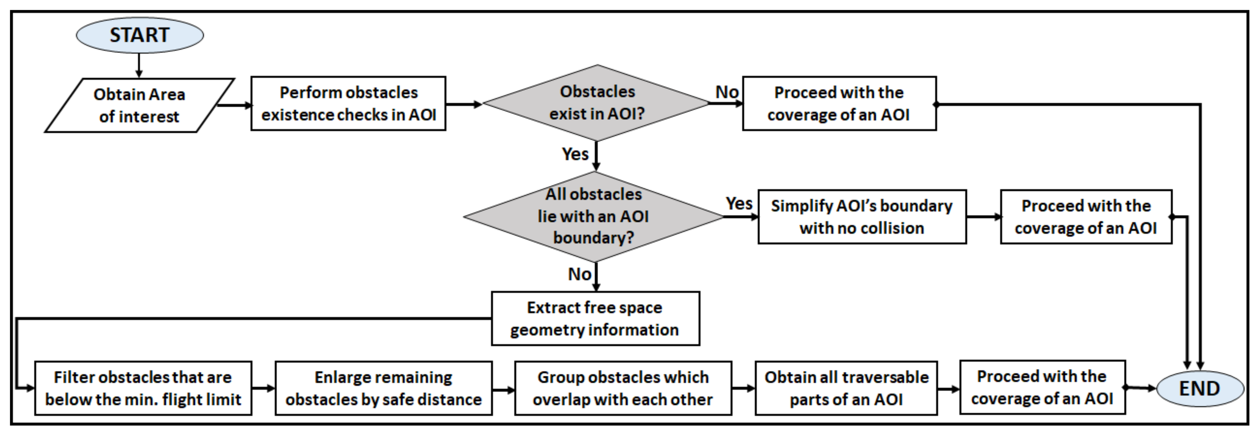
3.4.1. Multi-Criteria-Based Free Space Geometry Information Extraction from an AOI

Free space geometry information from an AOI can be extracted by a using multi-criteria-based method. Firstly, the obstacles’ existence checks are performed in an AOI by the line rotation method (i.e., a line $l_r$ is drawn from one vertex $p_i$ of an AOI to its nearest adjacent vertices $p_{i+1}$ and rotate it to all p vertices). Due to these checks, the AOI can be classified into three categories, (i) obstacle-inhibiting environment, (ii) obstacle-free environment, and (iii) area boundary obstacles only. In the third case, an AOI’s boundary is simplified by considering the nearby obstacles that intersect with the AOI vertices/edges or lying in very close proximity to it. The AOI’s boundary is modified by shrinking the AOI’s actual boundary inward, considering the UAV size and obstacles with whom UAV can possibly collide during the coverage mission. Later, the simplified environment is used for the coverage mission. The working of the multi-criteria-based free space geometry information extraction method is shown in Figure 5.

If no obstacles intersect with the $l_r$, then the AOI is regarded as the obstacle-free environment, and coverage can be performed with ease (i.e., second case). Meanwhile, if the obstacles exist in an AOI, the obstacles’ expansion (i.e., enlarging the obstacles’ intersections by a $D_{safe}$ value out of the obstacles) is carried out to avoid collision with obstacles. The nearby obstacles are clustered which overlap each other due to $D_{safe}$ addition. Furthermore, we cluster the obstacles which become very close to each other such that a UAV can possibly collide with them. The $D_{safe}$ is an integer number whose value can be determined/adjusted considering the operating environment, UAV size, and obstacles’ shapes. We apply the $H_{min}$ (where $H_{min}=$ minimum UAV altitude limits) to filter the obstacles that fall below the $H_{min}$, and the UAV can go over safely. Through the above-mentioned multi-criteria-based free space geometry information extraction method, the AOI can be classified into non-traversable and traversable parts. Subsequently, we fit the UAV’s sensor/camera footprints’ sweeps only in the traversal parts for the coverage missions after choosing the appropriate coverage direction(s).

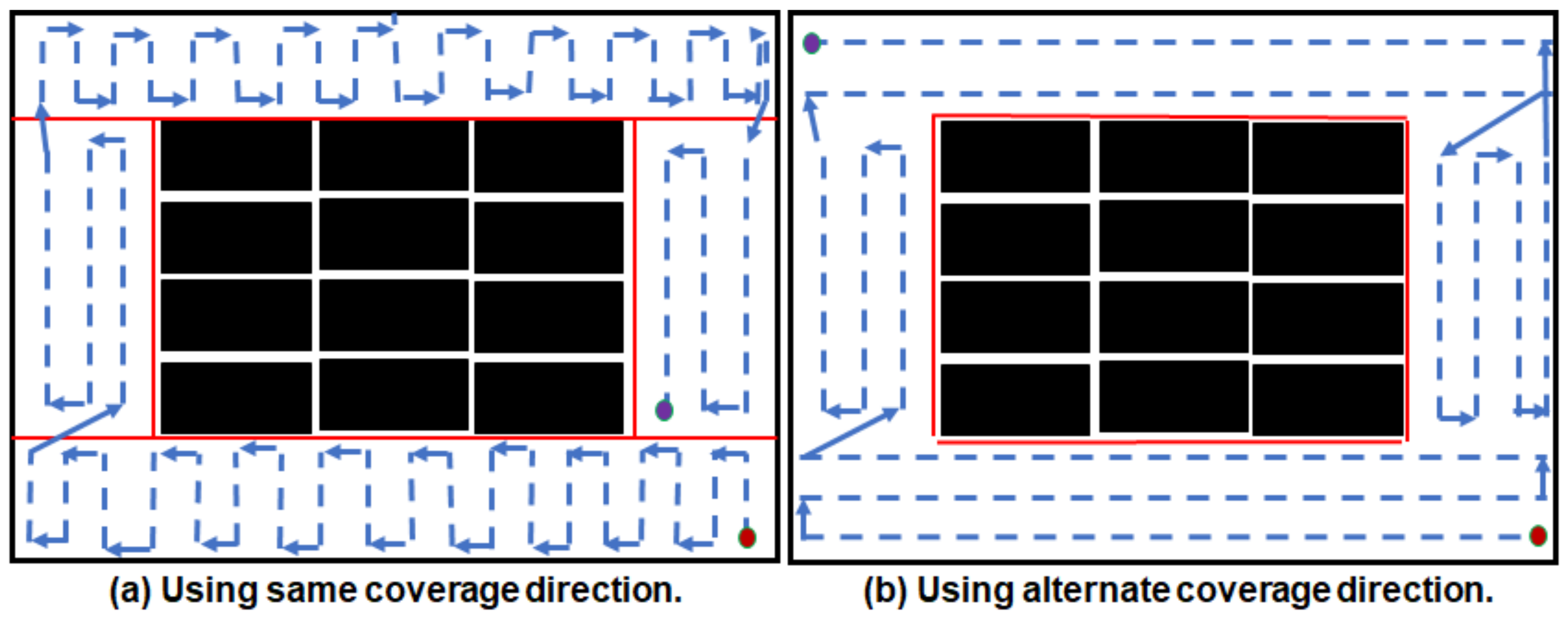
3.4.2. Choosing the Appropriate Coverage Direction(s) by Exploiting Available Free Space Geometry Information and Analyzing the Geometrical Characteristics of the AOI

Choosing the best coverage direction(s) has a range of advantages in coverage scenarios such as it lowers the turning maneuvers in a flight path to save the UAV resources. The turning maneuvers are very costly in terms of the energy consumption, coverage time, and path length because the UAV has to perform three actions for each turning maneuver such as (i) reducing the current speed, (ii) taking the turn, and (iii) increasing the speed again. Figure 6 demonstrates the overview of the coverage path obtained from the $Q_1$ with two different coverage directions. From the Figure 6b,c, it can be observed that coverage direction has a significant impact on the turning maneuvers, and it requires detailed knowledge regarding the underlying AOI in order to reduce the turns. The $\zeta$ in Figure 6b has only three turns while the $\zeta$ in Figure 6c has eleven turns.

In this paper, the best coverage direction (s) is determined by exploiting traversable parts’ geometry information, and analyzing the span W of the AOI to be covered with a UAV. In regular-shaped AOIs, we find the values of both the vertical span $W_v$ and horizontal span $W_h$ of the AOI for the best coverage direction selection. Furthermore, the AOI’s traversable parts’ geometry knowledge is exploited to select the most appropriate coverage direction (s). Meanwhile, the coverage direction is mostly chosen parallel to the maximal span axis and considering the tendency of free spaces. We employ single/multiple coverage directions depending upon the given AOI complexity to reduce the number of turns. Moreover, if an AOI is not in the regular shape, we transform it to a regular shape by the using convex-hull concept for the span calculation and, accordingly, the best coverage direction selection. If $W_v=W_h$, then the appropriate coverage direction can be chosen considering the obstacles placement and next AOI. In addition, by utilizing the global information of the AOI, and following the practical procedure explained above, the proposed CPP algorithm has the ability to find the best coverage direction, which in turn yields a smaller number of turning maneuvers in $\zeta$.

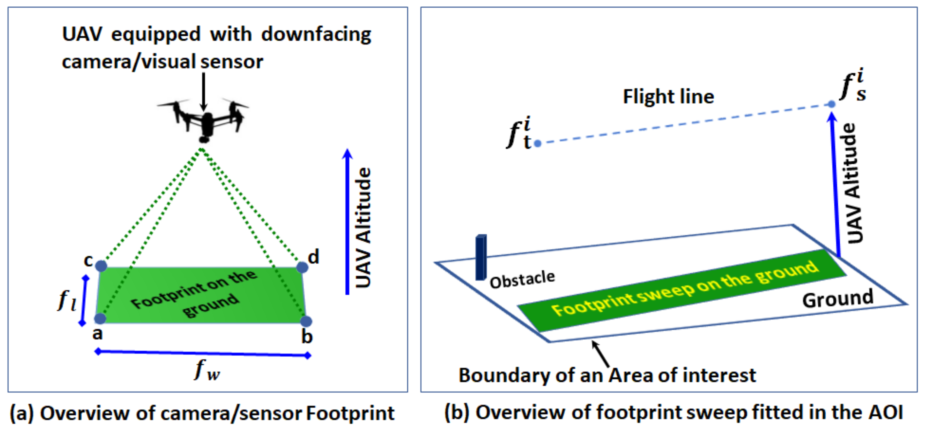
3.4.3. Fitting Sensor/Camera Footprints’ Sweeps in All Traversal Parts of the AOI

In coverage missions, a UAV always carries a specific tool which can be a transmitter, visual sensor, digital camera, or a spray tank depending upon the scenario. This tool is usually downward facing and mounted on the UAV. This work considers that the UAV carries a visual sensor/camera to cover the AOI for imagery missions. The attached tools with a UAV can have different characteristics related to sensing, and varying footprint sizes depending upon the UAV altitudes. For example, when the UAV altitude is low, image resolution is very high and footprint size is small, and vice versa. However, these sensing parameters/characteristics can be adjusted and are usually taken at the start of the mission. During tests, it is assumed that UAV generally flies at constant altitude while covering an AOI. However, in some cases, the priorities can be assigned to some parts of the AOI. The sensor footprint f is of rectangular shape with fixed width $f_w$ and length $f_l$, respectively. The sensor footprint size on the ground can be determined as shown in Figure 7a, and later N SFSs can be fitted in the traversable parts of an AOI in such a way that fewer footprints’ sweeps can achieve the coverage of most parts. The N SFSs fitted in an AOI can be mathematically expressed as set S as shown in Equation (9).

$$S=\{f_1,f_2,f_3,\cdots ,f_N\}.$$

(9)

Each SFS has two main parts: one is from a certain height (i.e., the 3D line segment form) which is also called the flight line and the other on the ground (i.e., the 2D rectangular form with four vertices ($a,b,c,d$), and fixed width $f_w$ and length $f_l$) similar to the sample given in Figure 7b.

The 3D line that passes from the middle of the ground footprint is used as an actual path on which UAV moves during the coverage mission. Considering the SFS as a line segment, the start point $f_s$ and endpoint $f_t$ of an $ith$ SFS are given as:

$$f_i=(f_s^i,f_t^i)=((x_s^i,y_s^i,z_s^i),(x_t^i,y_t^i,z_t^i)).$$

(10)

After fitting the SFSs in all required parts of the AOI, the midpoint of each footprint line segment part utilizing $f_s^i$ and $f_t^i$ values are computed. The objective is to find the visiting sequence of the SFSs by utilizing these midpoints. The midpoint $f_m^i$ of the ith footprint $f_i$ can be computed using the respective co-ordinates values of both $f_s^i$ and $f_t^i$. A detailed pictorial overview of a f in a rectangle form and SFS is shown in Figure 7b.

3.4.4. Determining the Visiting Sequence of the Footprints’ Sweeps by Formulating and Solving It as TSP

After fitting the sensor/camera footprints’ sweeps in the AOI, the next step is to determine the sequence/order in which the footprints’ sweeps will be connected and visited to ensure the perfect coverage of the AOI. To find the low-cost footprints’ sweeps visiting sequence, it is formulated as a TSP, and the ACO algorithm as explained earlier is employed to compute the visiting sequence. A pictorial overview of the TSP calculated from the 25 3D points (footprints’ sweeps’ midpoints) in 2D is shown in Figure 8.

Rigorous experiments are performed to verify the computed sequence. Through this process, a low-cost footprints’ sweeps visiting sequence can be obtained for further processing. For example, five footprints’ sweeps, $f_1$, $f_2$, $f_3$, $f_4$, $f_5$ can be processed via ACO and an optimal visiting sequence in the form $f_1$⇒$f_2$⇒$f_3$⇒$f_5$⇒$f_4$⇒$f_1$ can be obtained. We store the footprints’ sweeps visiting sequence information in set $\nu$, where $\nu =\{(f_1,x_1),(f_2,x_2),\cdots ,(f_n,x_n)\}.$. The x values in set $\nu$ denote the visiting sequence value of the respective f. The obtained footprints’ sweeps visiting sequence is used for SWG construction and coverage pathfinding, respectively.

3.4.5. Generation of the Sparse Waypoints Graph by Connecting the Endpoint of Footprints’ Sweeps

An SWG is generated by connecting the SFSs’ endpoints for the coverage pathfinding from an AOI. Mathematically, the SWG is a double edge graph $\omega$ of the reachable locations, $\omega =\{V,E\}$, where V represents the set of nodes, and E represents the set of edges. The V are basically the SFSs’ endpoints, while E are the straight lines for each SFS and connection from one sweep to another (i.e., circular form). Each sweep is a line segment with two endpoints $f_s$ and $f_t$ (i.e., $f_i=\overline{f_s^i{f}_t^i}$) as shown in Figure 7b. The SFSs’ endpoints are connected with the coincident (i.e., neighbors) sweeps’ endpoints to form $\omega$. Furthermore, the $\omega$ construction process encounters obstacles that need to be avoided while respecting the UAV maneuverability constraints. We devised a low cost strategy to avoid obstacles that hinder sweeps’ connection by evaluating and selecting the three avoidance options (i.e., left, right, top) as shown in Figure 9a. The footprints’ sweeps can be classified into two categories: (i) the maximal coverage sweeps, and (ii) partial coverage sweeps. The former sweeps are the ones which start from one corner of the AOI to the other without encountering any obstacle. In contrast, the later sweeps encounter obstacles and are not able to reach to the other end of the AOI. The pictorial overview of the partial and maximal coverage sweeps is shown in Figure 9b. The green and yellow colours represent the partial maximal coverage sweeps, respectively. The large number of maximal sweeps can enhance the convergence rate, and the path can be computed with least turns. Moreover, in obstacle-rich environments, the number of maximal coverage sweeps can be less and the CPP requires extensive computing.

Given set S of SFSs, where each sweep is in the form of a line segment with start point ($f_s$) and endpoint ($f_t$), collision-free connections between sweeps are determined to construct a SWG $\omega$. The complete pseudo-code used to generate $\omega$ from the AOI (i.e., $Q_i$) while avoiding obstacles safely is given in Algorithm 1. The proposed algorithm computes and selects the low-cost obstacle avoidance option from the three candidate options (shown in Figure 9a). To successfully avoid scattered obstacles present in an AOI, two additional points on all three sides of an obstacle are introduced, and the distance is computed for low-cost collision avoidance.

Algorithm 1. Sparse Waypoint Graph Construction from an AOI $Q_i$ located in an Urban Environment.

Input   :(1) $Q_i$ inhabiting N obstacles, where $N=\{o_1,o_2,o_3,\cdots ,o_n\}$ and each obstacle has random geometry.                (2) Set $\nu$ of sweeps’ visiting sequence, where $\nu =\{(f_1,x_1),(f_2,x_2),\cdots ,(f_n,x_n)\}.$                (3) Set S of the sensor footprints’ sweeps, where $s=\{f_1,f_2,\cdots ,f_n\}$ and $f_i=(f_s^i,f_t^i)$.   Output: Sparse waypoints graph $\omega$   Procedure:   1  for every sweep $f_i$, where $f_i$ = $f_1$ to $f_n$∈S do  2      Find the next sweep $f_j$ considering the the optimized visiting sequence (i.e., x values in set $\nu$).  3      Figure out the relevant endpoint pair using $(f_s^i,f_s^j,f_t^i,f_t^j)$ for the connection $c_i$  4      if INTERSECTS($c_i$,$o_k$) then  5         Evaluate the obstacle $o_k$ bypassing options values, $d_l,d_r,d_t$ using the following Equations.  6            Calculate $d_r$ for bypassing from the right: $d_r=d\{(f_s^i,f_t^i),p_{r_1})\}+d(p_{r_1},p_{r_2})+d\{p_{r_2},(f_s^j,f_t^j)\}$.  7            Calculate $d_l$ for bypassing from the left: $d_l=d\{(f_s^i,f_t^i),p_{l_1})\}+d(p_{l_1},p_{l_2})+d\{p_{l_2},(f_s^j,f_t^j)\}$.  8            Calculate $d_t$ for bypassing from the top: $d_t=d\{(f_s^i,f_t^i),p_{t_1})\}+d(p_{t_1},p_{t_2})+d\{p_{t_2},(f_s^j,f_t^j)\}$.  9         Select the appropriate obstacle $o_k$ bypassing option $AOB{O}_k$ using $AOB{O}_k=min(d_r,d_l,d_t)$, where           $d_r,d_l,d_t$ shows the minimum cost required to avoid $o_k$ from the right, left, and top, respectively.  10         Create collision free $c_i$ between sweeps $f_i$ and $f_j$ by acquiring the relevant endpoints.  11      else  12         Create collision free $c_i$ between sweeps $f_i$ and $f_j$ with the relevant endpoints.  13      End if  14   End for  15 return $\mathit{\omega }$

In Algorithm 1, the AOI $Q_i$ inhabits N obstacles, SFSs set S, and the SFSs’ visiting sequence set $\nu$ are given as an input. The SWG $\omega$, where $\omega =\{V,E\}$ is obtained as an output. Line 2 implements the finding of an appropriate SFS $f_j$ to be connected with an SFS $f_i$ from set S based on the optimized visiting sequence values stored in a set $\nu$. Line 3 implements the figuring out of the relevant endpoint’s pairs with the help of which a collision-free connection $c_i$ which can be established between $f_i$ and $f_j$. Line 4 performs the check for the possible obstacle(s) existence that can hinder the formation of a collision-free connection $c_i$. Lines 5–8 implement the cost/distance computation to avoid an obstacle $o_k$ from either the top, left or right using $o_k$, $f_i$, and $f_j$ geometry’s information. Line 9 implements the finding of a lowest cost obstacle avoidance option among the three candidate options. Line 10 implements the connection formation while avoiding obstacles present between SFSs $f_i$ and $f_j$. Line 12 implements the connection formation if no obstacles exist between two sweeps. When under the $if-else$ condition, Lines 4–13 perform the generation of the collision free connections with and without the presence of the obstacles. Furthermore, the same process is repeated for all sweeps until a complete SWG is constructed. Finally, an SWG $\omega$ is returned as an output (line 15). Furthermore, in some cases, the connection gap value is also taken as an input to be considered during the $\omega$ construction for turns handling depending upon the type of a UAV.

3.4.6. Intra-Regional Path Searching over the SWG to Fully Cover an AOI

After generating the $\omega$ from an AOI $Q_i$, the path searching is carried out to find an intra-regional path $\zeta$ from the UAV’s depot location (i.e., $v_s$). It is assumed that $v_s$ is very close to the $Q_i$, and no obstacles exist between the $v_s$ and starting location $b_i$ of the $Q_i$. The location in which UAV finishes the perfect coverage of an $Q_i$ is denoted with $e_i$. The $e_i$ location is used to make decisions in switching between areas. After complete $\omega$ construction, the path searching process begins from the point $v_s$ and continues until the perfect coverage is achieved. To find an intra-regional collision-free path ${\zeta }_i$ over an SWG constructed from the $Qi$ located in an urban environment, we employed the ACO algorithm which generated the optimized visiting order of the SFSs, and informed the search. Our algorithm maintains the track of the locations to be visited by a UAV using the order generated by the ACO for SFSs connections. It is assumes that UAV is able to execute turning maneuvers with sufficient accuracy while transiting from one sweep to another during the coverage mission. The complete pseudo-code is used to find ${\zeta }_i$ from $Q_i$) without sacrificing the guarantees on the stated assertions is given in Algorithm 2.

Algorithm 2. Coverage pathfinding to fully scan a target area $Q_i$ with a UAV-mounted Sensor/Camera.

Input   :(1) The depot location $v_s$ of the UAV, where $v_s=(x_s,y_s,z_s)$.                (2) Set $\nu$ of the sweeps’ visiting sequence, where $\nu =\{(f_1,x_1),(f_2,x_2),\cdots ,(f_n,x_n)\}.$                (3) Sparse waypoints graph $\omega$ of the sweeps connections, where $\omega =\{V,E\}$.                (4) The starting location $b_i$ of the mission in the AOI, where $b_i=f_s^i=(x_s^i,y_s^i,z_s^i)$  Output  :Intra-regional path ${\zeta }_i$ and mission end location $e_i$  Procedure:  1   Connect the UAV’s depot location $v_s$ with the starting location $b_i$ of the mission in the AOI with a line $l_e$.  2   for every sweep $f_i$, where $f_i$ = $f_1$ to $f_n$∈$\omega$ do  3      Find the next sweep $f_j$ considering the the optimized visiting sequence (i.e., x values in set $\nu$).  4      Find the connection $c_i$ which connects the $f_i$ and $f_j$ in $\omega$  5      Traverse all the nodes and lines of the $f_i$, $f_j$, and $c_i$ in a BF manner, and record this as $r_1$.  6      Repeat: steps 3–5 for the next sweep $f_k\in \omega$, where $f_j$ is the successor sweep of $f_k$.  7      Traverse all the nodes and lines of the $f_j$, $f_k$, and $c_{i+1}$ in a BF manner, and record this as $r_2$.  8      if lastRound($f_k$,$f_n$) then  9         Traverse all the nodes and lines of the $f_k$, $f_n$, and $c_{i+n}$ in a BF manner, and record this as $r_n$.  10         Assign the endpoint of the $r_n$ to the $e_i$.  11      else  12         Repeat: ∀$\{f_l,f_m,f_n,\cdots ,f_n\}\in \omega$, find all respective rounds.  13         Assign the endpoint of the $r_n$ to the $e_i$.  14      End if  15      Add the path information in ${\zeta }_i$, where ${\zeta }_i=\{l_e,(r_1,r_2,r_3,\cdots ,r_n)\}$.  16   End for  17 return ${\zeta }_i$ and $e_i$

In Algorithm 2, the UAV depot location $v_s$, SFSs set S, and SFSs’ visiting sequence set $\nu$, SWG $\omega$, and starting location $b_i$ which is the point of entry in $Q_i$ are given as an input. The path ${\zeta }_i$ and mission end location $e_i$ are obtained as an output. Line 1 implements the connection establishment between the $v_s$ and $b_i$. Lines 3–5 implement the first complete round formation in a BF manner using the two SFSs ($f_i$ and $f_j$) and their connection ($c_i$). Lines 6–7 implement the the second complete round formation in a BF manner using the two SFSs ($f_j$ and $f_k$) and their connection ($c_{i+1}$). Lines 8–14 determines whether the perfect coverage has been achieved or not via if−else conditions; in both cases, the location where the mission finishes is recorded (Lines 10 and 13). The complete coverage path information is stored in ${\zeta }_i$ (Line 15). Finally, path information along with the mission completion location is returned as an output (line 17). Our CPP algorithm finds the path very quickly since the already optimized visiting order and informed search strategy is utilized. Furthermore, the $\omega$ contains fewer nodes and edges, and thereby the path searching time is significantly lower, and ${\zeta }_i$ can be computed quickly.

3.5. Determining the Next Area of Interest to Switch from the Current Area of Interest with the Lowest Possible Cost

After the perfect coverage of an AOI $Q_i$ with the path ${\zeta }_i$, the next AOI $Q_j$ to be covered is determined. Although the traversal order for each AOI’s visits is determined in advance but it cannot lead to optimal results in some cases. Therefore, the appropriateness of traversal order is re-assessed while switching between different AOIs. The two cases in which the traversal order can/cannot yield the appropriate results are presented in Figure 10. As shown in Figure 10ii, the cost of switching from $Q_2$ to $Q_1$ as per the ACO algorithm’s suggested order is more than $Q_2$ to $Q_3$ based on the coverage path end location. Hence, in such cases, the traversal order is re-evaluated and modified if required to lower the overall path cost. In such cases, the intra-regional and inter-regional path computation cannot be separated. Concisely, if the AOIs are not well separated, the traversal order computed at the start may yield longer paths. This work resolves this problem by analyzing the distances between the AOIs. If the distance between all AOIs is sufficiently large, then the traversal order computed at the start can yield optimal results in most cases as shown in Figure 10i. However, if the AOIs are not well-separated, then the traversal order computed at the start can no longer yield feasible results, and re-assessment of the traversal order is needed as shown in Figure 10ii. The main reason behind this problem is the intra-regional path that can impact traversal order based on the mission completion locations in a respective AOI.

Once, the decision about the next AOI is made, the low-cost path is determined for switching from the current AOI to the next AOI. We formalize and solve it as a traditional PP problem between two pre-determined locations.

3.6. Switching to the Next AOI by Formulating and Solving It as a Traditional Path Planning Problem

To safely switch from the end location $e_i$ of an AOI $Q_i$ to the start location $b_j$ of an AOI $Q_j$, a five-step process was devised. The whole process is formalized as a traditional path planning problem in which $e_i$ and $b_j$ are perceived as the source and target locations, respectively. The objective is to find the shortest path $W_{ij}$ in a 3D urban environment between two points,$e_i$ and $b_j$, avoiding obstacles present in an underlying environment. The nodes set of the path ($W_{ij}$) has two characteristics, (i) $W_{ij}\in X_{free}$ and (ii) $W_{ij}\cap X_{obstacles}=\varnothing$. The functional model between $e_i$ and $b_j$ for the two-PP objective optimization is as follows:

$$\left\{\begin{array}{c}{W}_{ij}=[e_i=w_{i{j}_1},w_{i{j}_2},w_{i{j}_3},\cdots ,w_{i{j}_n},w_{i{j}_n+1}=b_j]\hfill \\ Minimize{f}_1\left(W_{ij}\right)=ComputingTime\left(W_{ij}\right)\hfill \\ Minimize{f}_2\left(W_{ij}\right)=Length\left(W_{ij}\right)\hfill \end{array}\right.$$

The proposed algorithm effectively resolves the two conflicting goals by exploiting the obstacles’ geometry information, and UAV the is assumed as a single point in this work. The process employed to compute the $W_{ij}$ by fulfilling the two objectives is comprised of following five steps: (i) drawing straight line $l_0$ between two locations (i.e., $e_i$ and $b_j$), (ii) filtering the obstacles that intersect with the axis $l_0$, (iii) finding the initial path $W_{ij}^{{}^{\prime }}$ by exploiting the relevant obstacles geometry information, (iv) refining the initial path by clustering obstacles, and utilizing the straight line’s point of intersection information, and (iv) path following to reach to $Q_j$ from the $Q_i$ (i.e., inter-region switching).

3.6.1. Drawing Straight Line from the Exit Location of the Previous AOI to the Beginning Location of the Next AOI

At the beginning, a straight line $l_0$ is drawn from the exit location $\left(e\right)$ of the previous AOI to the beginning location (b) of the next AOI. For example, when $l_0$ is drawn from $e_i$ of an $ith$-AOI to the $b_j$ of the $jth$-AOI for an inter-AOI switching, three types of the results can be observed. All three are results visually presented in Figure 11. In the first two scenarios, the $l_0$ does not intersect the obstacles, and $l_0$ can be used as working path for switching (i.e., $l_0=W_{ij}$). Meanwhile, in the second scenario, there are some obstacles which lie very close to the $l_0$ and the UAV can possibly collide with them. Therefore, slight adjustments are performed in $l_0$ by considering nearby obstacles to find a $W_{ij}$ for inter-region switching. The third scenario is a typical PP problem, and it requires further processing since $l_0$ intersects with obstacles either from the middle or the corners. In this scenario, the further processing is carried to find the $W_{ij}$ by filtering the intersected obstacles and analyzing their geometry information. The detailed procedure to find $W_{ij}$ is described in the subsequent Section 3.6.2, Section 3.6.3, Section 3.6.4 and Section 3.6.5.

3.6.2. Filtering the Obstacles That Intersect with the Straight Line

In the third scenario, as shown in Figure 11c, two obstacles intersect with the $l_0$, and we need to avoid them while switching from the $e_i$ to $b_j$ locations. Consequently, such obstacles are filtered from the 3D urban environment map, and further processing is applied. The complete pseudo-code used to filter obstacles that intersect with the $l_0$ from the map is given in Algorithm 3. In Algorithm 3, urban environment map M encompassing N number of obstacles, mission end location $e_i$ of an $ith$ AOI, and mission beginning location $b_j$ of the $jth$ AOI are provided as an input. Set ℜ, where (ℜ⊆N) of relevant obstacles is yielded as an output. Line 2 implements the $l_0$ drawing between two locations $e_i$ and $b_j$. Lines 3–7 perform the filtering of the obstacles that intersect with the $l_0$. Finally, set ℜ of the relevant obstacles is returned (line 8). Meanwhile, if no obstacle lies between the two locations, then $\Re =\varnothing$ will be returned as an output.

Algorithm 3. Filtering relevant obstacles from the urban environment map.

Input   :(1) Urban environment map M containing N number of obstacles, where $N=\{o_1,o_2,o_3,\cdots ,o_n\}$                (2) Mission end location ($e_i$) of an $ith$ AOI                (3) Mission beginning location $b_j$ of the $jth$ AOI  Output:  Set ℜ of the filtered relevant obstacles  Procedure:  1 Initialize:, set ℜ = ∅  2 Draw straight line $l_0$ between ($e_i$) and ($b_j$)  3   for each $o_i$, where $o_i$ = $o_1$ to $o_n$∈N do  4      if INTERSECTS ($l_0$, $o_i$) then  5         $\Re =\Re \cup \left\{o_i\right\}$  6      End if  7   End for  8 return ℜ

After obtaining set ℜ of the relevant obstacles, we enlarge the filtered obstacles by the safe distance ($D_{safe}$). After that, we analyze the obstacles’ geometry that are on the $l_0$ between $e_i$ and $b_j$ to find a low cost $W_{ij}^{{}^{\prime }}$.

3.6.3. Finding the Initial Path by Exploiting the Filtered Obstacles’ Geometry Information

We find the initial (i.e., coarse) path $W_{ij}^{{}^{\prime }}$ for inter-region switching by considering the obstacles lying on $l_0$. Mathematically, $W_{ij}^{{}^{\prime }}$ can be expressed as:

$$W_{ij}^{{}^{\prime }}=d_{l_0}+\sum _{i=0}^N{D}_i$$

(11)

where $d_{l_0}$ represents the straight line distance d between two locations ($e_i$ and $b_j$), computed as $d_{l_0}=\sqrt{{(x_t^i-x_s^j)}^2+{(y_t^i-y_s^j)}^2+{(z_t^i-z_s^j)}^2}$, $D_i$ is the degradation in straight line path caused by the obstacles lying on the $l_0$, and $W_{ij}^{{}^{\prime }}$ is an initial path which is subsequently optimized. The degradation (D) in path length due to an obstacle (e.g., i) is calculated using Equation (12).

$$D_i=min(\frac{O_w}{2},O_h)$$

(12)

where $O_w$ and $O_h$ are the obstacle’s width and height, respectively.

This indicates three options for bypassing an obstacle. This work does not consider the hanged obstacles; therefore, there are only three options to avoid each obstacle. If there is no obstacle between $e_i$ and $b_j$, then, the second term in Equation (11) will be zero, and $W_{ij}^{{}^{\prime }}=d_{l_0}$. The path complexity $C_{W_{i}j}$ is mathematically expressed in Equation (13).

$$C_{W_{i}j}=\frac{d_{l_0}}{W_{ij}^{{}^{\prime }}}$$

(13)

where $d_{l_0}$ and $W_{ij}^{{}^{\prime }}$ show the length of the path without and with obstacles’ presence, respectively. The $C_{W_{i}j}$ value close to one is preferred. If a large number of obstacles exist between the two locations, the D value will be higher, and consequently $C_{W_{i}j}$ will be close to zero, and vice versa. Meanwhile, the $C_{W_{i}j}$ value is optimized more by exploiting obstacles’ geometry information to find the actual path $W_{ij}$.

3.6.4. Refining the Initial Path by Clustering Nearby Obstacles, and Utilizing the Straight Line’s Point of Intersection Information

After finding the initial path $W_{ij}^{{}^{\prime }}$, its length is optimized by exploiting the obstacle’s geometry information that is lying on the $l_0$. In order to lower the $C_{W_{i}j}$, obstacles that are lying close to each other are grouped to be considered as one obstacle. This helps in reducing the path length and number of turns in the path. Furthermore, the actual point of intersection with obstacles is taken into account rather than assuming that $l_0$ intersects each obstacle from the middle. By jointly using the accurate point of intersection information, and grouping the nearby obstacles, the path length is significantly shortened. The initial path $W_{ij}^{{}^{\prime }}$ becomes the working path $W_{ij}$, and it will be followed by the UAV for inter-region switching. In the path-refining phase, the main objective is to shorten the path’s length, and make it smooth to the greatest extent possible.

3.6.5. Path following for Inter-Region Switching

Once the $W_{ij}$ is determined, the UAV moves from one AOI to another. The UAV switches to the next AOI based on the traversal order and computed path. In the inter-region path computation, no attention is paid to the coverage and it is assumed that the UAV camera/scanner is off during the region’s switching. This work assumes zero-wind scenarios, and that the UAV has the ability to follow the computed path with sufficient accuracy. After switching to the AOI, the intra-regional path computing process begins as explained earlier in Section 3.4.1. The intra-and inter-regional path computation process carries on until the completion of all N AOI coverage. At the end, the $\mathsf{\Gamma }$ is returned, which is the working path for the mission. The $\mathsf{\Gamma }$ is the combination of both inter-and intra-regional paths which can be mathematically expressed as Equation (14).

$$\mathsf{\Gamma }=\{l_e,{\zeta }_1,W_{12},{\zeta }_2,W_{23},{\zeta }_3,W_{34},\cdots ,W_{(n-1)\left(n\right)},{\zeta }_n\}$$

(14)

where $l_e$ is the path from $v_s$ to the first AOI, and ${\zeta }_i$ and $W_{\left(i\right)(i+1)}$ represent the intra-and inter-regional paths, respectively. The $\mathsf{\Gamma }$ is a path for the full tour, and ensures the perfect coverage of all AOIs with low cost switching between AOIs during the coverage mission.

4. Experimental Evaluation and Discussion

This section presents the experimental results obtained from various representative scenarios, and their comparisons with the existing CPP algorithms. The improvements of the proposed CPP algorithm were compared from two different perspectives, singular AOI, and multiple AOI coverage. For the former case, the proposed algorithm’s effectiveness was evaluated using four metrics; (i) the improvements in computation time, (ii) path overlapping, (iii) path lengths, and (iv) the number of turning maneuvers. In the latter case, its effectiveness was evaluated using two metrics; (i) the improvements in computing time and (ii) path length. To benchmark our algorithm, we compared its results with a decomposition-based CPP method named the CA-CPP algorithm [63], and a dynamic programming-based CPP method named TSP-CPP [80]. The simulation results were generated and compared on a PC running Microsoft Windows 10, with a CPU Intel Core i5 with 2.6 GHz and 8.00 GB memory, using MATLAB version 9.8.0.1359463 (R2020a). In simulations, both global constraints that are related to the operating environment (i.e., urban environment in our study), and local constraints that are related to the UAV configuration and structure were considered. The numerical/non-numerical values related to both constraints are summarized in

Table 2. Numerical/Non-numerical values of the global (urban environment) and local (UAV itself) constraints.

Constraints Type	Constraint Name	Constraints Values
		Numerical	Non-Numerical
Local	Wing span UAV size Steering angle Wind’s affect Available energy/battery Footprint sweep’s width Footprint sweep’s length Maximum UAV flight height limits Minimum UAV flight height limits	1 m 25 kg $\frac{\pi }{6}$ radius - - 20 m 30 m 155 m 25 m	- - - No-affect (zero-wind scenarios) Sufficient for whole coverage mission - - - -
Global	UAV workspace Obstacle’s geometry information Obstacles’ placement and sizes Safe distance from obstacles	- - - - 10 m	Urban areas Fully-known Random -

.

The performance comparisons of our algorithm are presented in the following subsections.

4.1. Performance Comparisons of the Proposed CPP Algorithm in Singular AOI Coverage

The overview of the 3D maps used in the simulations experiments and an exemplary coverage path computed by the proposed CPP are visually presented in Figure 12. We compared our algorithm’s results with the existing CA-CPP method by (i) varying obstacles’ complexity and (ii) the shape of the AOI. The relevant details about the obtained results are described in the respective subsections.

4.1.1. Comparisons with the Existing CPP Algorithm Based on Obstacles’ Complexities

The obstacles’ number and their placement in an AOI significantly impact the performance of any CPP algorithm. To validate the proposed CPP algorithm feasibility for coverage missions in 3D urban environments, we compared our algorithm’s computing time, path lengths, number of turning maneuvers, and path overlapping results with the existing method using five maps with varying obstacles’ complexities. Obstacles’ complexity is referred to as the density of the obstacles. The proposed CPP algorithm performance is compared using three obstacles’ density values (e.g., low, medium, and high) on the regularly shaped AOI. The complete description about the AOI sizes used in the simulation experiments, obstacles’ densities, and average running time and path length result comparisons of the proposed CPP algorithm are shown in

Table 3. Description of the AOI and the proposed algorithm CPP results in comparison with the CA-CPP method.

Map id	Area of Intrest Size	Obstacles Density	CA-CPP Algorithm [63] Results		Proposed-CPP Algorithm Results
			Avg. Computing Time (s)	Avg. Path Length (m)	Avg. Computing Time (s)	Avg. Path Length (m)
Map 1	500 × 600 × 300	Low Medium High	6.07 11.47 20.49	9518.08 8460.47 7609.68	5.04 9.58 17.01	9152.50 8135.40 7317.19
Map 2	1000 × 1200 × 300	Low Medium High	10.15 20.22 26.32	40,665.13 35,753.12 34,278.49	8.48 16.53 21.93	38,914.02 34,378.51 32,960.98
Map 3	1200 × 1400 × 300	Low Medium High	13.45 22.40 29.81	57,830.31 56,047.68 52,140.4	11.24 18.72 24.91	55,340.24 53,892.23 50,130.08
Map 4	1500 × 1500 × 400	Low Medium High	18.09 26.72 35.76	76,504.45 72,846.82 72,644.25	15.12 22.33 29.88	73,210.21 70,040.32 69,840.89
Map 5	2000 × 2000 × 400	Low Medium High	20.41 33.50 37.92	133,866.59 126,360.78 122,304.78	17.05 27.88 31.54	128,100.45 121,400.11 117,500.92

.

In experimental evaluation, all obstacles were placed randomly in an AOI. If the obstacles’ density is low, it means that AOI has a smaller number of obstacles, and consequently most parts of the AOI can be traversed. In contrast, the AOI with the high density of obstacles has fewer traversable parts, and the path overlapping can increase due to the complex obstacle geometry. The areas with medium density have uniform distribution of obstacles, and almost half of the spaces can be covered with the SFSs. The proposed CPP algorithm does not decompose the AOI into blocks/cells which can lead to excessive path overlapping and very high computing time in complex scenarios. Meanwhile, the CA-CPP method [63] decomposes the AOI into cells and find a coverage path. This algorithms is suitable for coverage missions, but the small-sized cells obtained through decomposition can cause path length degradation. In most cases, the computing time increases exponentially with the problem size (i.e., AOI size, and obstacles’ geometries). Our algorithm incurs less computing time by using SFSs and SWG with the minimum nodes and edges to accomplish the complete coverage task.

From the results, it can be observed that the computing time increases with an increase in obstacles’ densities and the size of the AOI. However, the path length in each case decrease with an increase in obstacles’ densities. Moreover, our algorithm shows a 20.09% reduction in the computing time compared to the prior algorithm. From the path length point of view, the proposed algorithm shows a 4.39% reduction compared to the CA-CPP algorithm. Meanwhile, in some cases, when the environment complexity is low or the AOI size is small (i.e., the first two cases), the CA-CPP algorithm yields the shortest length path compared to the proposed algorithm. Meanwhile, as the AOI size and obstacle densities increase, the performance of our algorithm improves on both metrics (i.e., computing time and path lengths). The significant improvements in computing time and path lengths are due to the sensor range-aware footprints’ sweeps fitting that guarantees maximal coverage with fewer sweeps. Our algorithm’s path overlapping and turning maneuvers results with the prior algorithm in each map (listed in Table 3) were compared, and corresponding results and their comparison are shown in

Table 4. Path overlapping comparison between three algorithms for the same area of interest.

Coverage Algorithms	Evaluation Criteria	Map id (Area of Interest Size)
		1 (500 × 600 × 300)	2 (1000 × 1200 × 300)	3 (1200 × 1400 × 300)	4 (1500 × 1500 × 400)	5 (2000 × 2000 × 400)
CA-CPP Algorithm [63]	Avg. path overlapping (m) Avg. number of turning maneuver	119.09 116	278.07 210	1090.15 223	1351.08 238	2079.11 318
Proposed CPP algorithm	Avg. path overlapping (m) Avg. number of turning maneuver	160.69 104	291.72 199	911.85 211	1223.02 227	1967.05 316

.

The proposed algorithm on average gives 7.92% and $5.34\%$ improvements in path overlapping and turning maneuver results compared to the prior algorithm on five different maps of varying obstacle densities and AOI sizes. Furthermore, it ensures the coverage ratio $c_{ratio}$ of 1.0 that represents perfect coverage (i.e., 100%) of an AOI.

4.1.2. Comparisons with the Prior CPP Algorithm Based on the Shape of the Area of Interest

Besides the obstacle’s densities, the shape of the AOI is also a relevant factor that can significantly impact performance of any CPP algorithm. CPP over a regularly shaped AOI is relatively easier compared to that for an irregularly shaped AOI. In a regularly shaped AOI, coverage can be performed with the help of a simple BF pattern. Moreover, in an irregularly shaped AOI, the coverage requires concavity modification, and hybrid motion patterns are needed to achieve full coverage. The CPP complexity varies with the shape of the AOI, and to find a low-cost path obstacles’ geometry knowledge to the fine-grained level is required. To this end, we compared our algorithm performance with the existing methods over five different types of AOI. We performed rigorous experiments to verify the algorithm performance in relation to the shape of the AOI. The average results of path length, computation time, turning maneuvers, and path overlapping are shown in

Table 5. Comparison of the proposed algorithm performance with varying shapes of the area of interest.

Coverage Algorithms	Shape of the Area of Interest	Evaluation Criteria (s)
		Avg. Path Length (m)	Avg. Computing Time (s)	Avg. Path Overlapping (m)	Avg. Turning Maneuvers
CA-CPP Algorithm [63]	Square Rectangle Polygon (convex) Polygon (non-convex) Irregular	70,904.37 8451.67 52,000.22 55,824.41 48,762.62	28.36 13.84 22.03 32.21 21.205	1259.31 179.35 684.88 775.35 988.91	51 55 52 95 103
Proposed CPP Algorithm	Square Rectangle Polygon (convex) Polygon (non-convex) Irregular	67,220.92 7905.12 51,098.11 53,915.78 46,591.09	17.15 8.88 15.19 21.91 13.10	1041.22 164.09 614.04 701.05 948.31	35 45 47 79 84

.

Through simulations and comparison with the prior algorithm using five distinct shapes of the AOI, on average, our proposed algorithm reduces the computing time of coverage path-finding by 19.24%. From a path length and path overlapping point of view, it reduces path length by 3.90% and path overlapping by 10.77%, respectively. Additionally, the proposed CPP algorithm reduces turning maneuvers by 9.26%. These results emphasize the proposed algorithm’s effectiveness in all four criteria.

4.1.3. General Comparisons of the Proposed Algorithm with the Existing CPP Algorithms

Apart from the numerical result explained above, the proposed CPP algorithm has several more advantages compared to the existing CPP methods. Four potential advantages of the proposed CPP algorithm that can highlight the utility of our algorithm for practical scenarios in urban environments are summarized below.

A. Compared with the previous solution in terms of the improved solution quality: in the literature, several exact cellular decomposition-based algorithms employ the same coverage direction in each subarea after decomposition of an AOI [16]. Using same coverage direction in each subarea is highly inefficient when the map complexity is high. In contrast, our CPP algorithm uses an alternate coverage direction by capturing the notion of free spaces to achieve maximal coverage with fewer SFSs. Figure 13 shows the comparison of two methods with the same and alternate coverage directions. Our algorithm fits sweeps of longer lengths to achieve better coverage. Additionally, the proposed algorithm path has the smallest number of turns and improved solution quality compared to the prior algorithms which employ same coverage direction in each decomposed area.

B. Compared with the previous solution in terms of transition distance between subareas: Most decomposition-based methods involve two types of the optimization in CPP: intra-cell and inter-cell [29]. In the latter optimization, it is desirable to consider the exit point of the previous cell/subarea and entrance point of the next cell/subarea simultaneously. However, most of the algorithms use pre-determined exits and entrance locations for subarea switching. Using the pre-determined entrance and exits locations can reduce the length of a path inside each cell/subarea up to some extent. However, the transition distance to switch from one subarea to another can increase drastically. Figure 14 shows the comparison of transition distance between subareas and the footprints’ sweeps connection. The red line shows the transition distance for both methods. Our algorithm shown in Figure 14b has a lower switching cost compared to the prior decomposition-based methods Figure 14a. Furthermore, it has less path overlapping than existing CPP methods in most cases.

C. Compared with the previous solution in terms of the number of way-points: The grid-based methods decompose the AOI into smaller grids of varying sizes and shapes [26]. Each grid can be either free or occupied by obstacles as shown in Figure 2b. Later, the graph is constructed from the middle of the obstacle-free grids, and an optimization algorithm is used to find the coverage path. The complexity of the CPP problem rises steadily with the increase in the number of nodes and edges obtained through the grids. Figure 15 shows the number of waypoints generated by our algorithm and existing grid-based methods for the same size of the AOI. From the results, it can be observed that the proposed algorithm has the smallest number of waypoints compared to the grid-based methods. Therefore, the proposed algorithm has the least computational complexity.

D. Compared with the previous solution in terms of perfect coverage of AOI: the decomposition-based methods decompose the AOI into smaller cells of varying sizes/ shapes [64]. Each cell has distinct geometry as shown in Figure 16a. Depending upon decomposition type, many traversable places of an AOI cannot be scanned fully if SFs are not considered during CPP process. Hence, in most cases, the prior CPP algorithms do not guarantee the coverage ratio $c_{ratio}$ of 1.0 that refers to perfect coverage (i.e., 100%). As shown in Figure 16a, some traversable parts are not covered by the BCDH-CPP [64]. However, our algorithm considers the SF on the ground from the desired UAV altitude. Therefore, in most cases, our algorithm guarantees the coverage ratio $C_{ratio}$ of 1.0 (i.e., 100%) of an AOI. From the results, it can be observed that our algorithm can achieve perfect coverage of an AOI with fewer turns than the prior method. Therefore, the proposed CPP algorithm has better utility for practical scenarios than the existing CPP methods.

4.2. Performance Comparisons of the Proposed CPP Algorithm in Multiple AOI Coverage

This subsection discuses the detailed results in multiple AOI coverage. Two metrics computing time and path lengths are chosen to evaluate our algorithm effectiveness over the existing algorithm in multiple CPP scenarios. The results are compared with the TSP-CPP algorithm [80]; it is the only available algorithm until now for the coverage of multiple regions. The overview of the 3D maps used in the experiments, and an exemplary coverage path computed by the proposed CPP for covering multiple AOIs, is visually presented in Figure 17. In Figure 17a, four rectangular-shaped AOIs are marked with the red boundary. In Figure 17b, the green part shows the sensor scan on the ground, and blue lines represent the upper portion of the sweeps from a certain altitude as shown in Figure 17b. The SWG is shown in Figure 17c, which is obtained by connecting sweeps. Finally, the complete coverage path obtained from four spatially distributed AOIs is sown in Figure 17d. In the next subsections, our algorithm results were compared with the prior algorithm by (i) varying AOI counts and (ii) the sizes of each AOI.

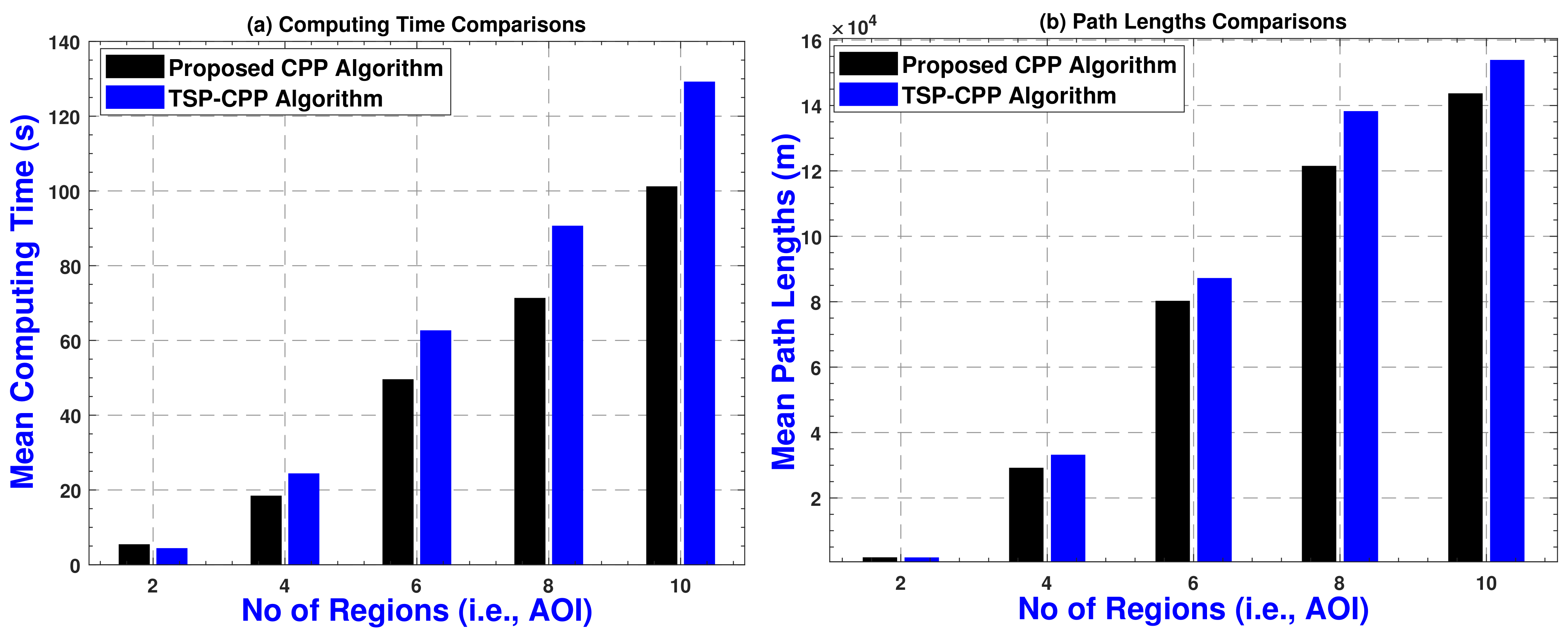
4.2.1. Comparisons with the Prior CPP Algorithm Based on Counts of the Area of Interest

The number of the AOIs can increase the complexity of the CPP algorithm due to the inclusion of excessive operations/calculations. Furthermore, the obstacles’ presence and their capricious placement in the AOI can further complicate the CPP process. To evaluate the performance, the number of AOIs (i.e., regions) was varied, and five scenarios were considered: (i.e., $N=\{2,4,6,8,10\}$). All AOIs are of the convex-polygonal shape, and are randomly generated, not overlapping with each other. We evaluated the performance via efficiency and optimality, and compared the results with TSP-CPP [80]. Although the TSP-CPP algorithm [80] was tested on large number of regions, all the regions were obstacle-free. The average computing time and path length results obtained from the experiments are shown in Figure 18. These results are the average of five runs in each test. From the results, it can be seen that our algorithm performs consistently better than the TSP-CPP algorithm. Although both time and length increase with number of AOIs, our algorithm reduces both metrics at the same time. Our algorithm, on average, reduces the computing time by 20.99%, and path length by 9.10% than TSP-CPP algorithm. Beside the improvements in numerical results, it has the least space complexity due to lesser SFSs.

4.2.2. Comparisons with the Prior CPP Algorithm Based on Sizes of the Area of Interest

The size of an AOI is an important factor in evaluating any CPP algorithm’s performance. A small-sized AOI can be covered quickly, and vice versa. To this end, rigorous comparisons were made by varying the sizes of the AOI in each test. Three scenarios were considered regarding the variation of the sizes of the AOIs (i.e., regions): small-sized, medium-sized, and large-sized AOI. In addition, we consider five scenarios: $N=2$, $N=4$, $N=6$, $N=8$ and $N=10$ of the AOI’s counts along with their sizes. The test results obtained from the experiments, and their comparison with the TSP-CPP algorithm [80] are shown in

Table 6. Computing time and path length comparisons between CPP algorithms by varying AOI sizes.

AOI Sizes	Evaluation Criteria	Coverage Algorithms	Number of the Areas of Interest (i.e., Regions) Located in Urban Environments
			2	4	6	8	10
Small-sized	Computing Time, Path Length	TSP-CPP Algorithm [80] Proposed CPP algorithm	2.9 s, 1505.32 m 3.27 s, 1519.92 m	11.76 s, 2039.56 m 8.52 s, 1921.12 m	18.25 s, 2832.23 m 13.67 s, 2532.23 m	27.32 s, 3656.23 m 19.32 s, 3023.45 m	35.81 s, 4123.45 m 25.21 s, 3412.34 m
Medium-sized	Computing Time, Path Length	TSP-CPP Algorithm [80] Proposed CPP algorithm	5.69 s, 1815.12 m 6.27 s, 1829.12 m	16.61 s, 2409.06 m 12.32 s, 2321.02 m	26.59 s, 3372.13 m 20.56 s, 3052.23 m	39.72 s, 4506.21 m 30.92 s, 4003.15 m	55.01 s, 5313.95 m 41.28 s, 4902.14 m
Large-sized	Computing Time, Path Length	TSP-CPP Algorithm [80] Proposed CPP algorithm	10.19 s, 2319.02 m 11.87 s, 2321.19 m	25.01 s, 2999.16 m 20.52 s, 2901.12 m	37.95 s, 4170.03 m 30.51 s, 3852.93 m	54.02 s, 5500.31 m 44.02 s, 5010.05 m	76.91 s, 7123.02 m 60.31 s, 6512.24 m

. From the results given in Table 6, it can be observed that both path length and computing time increase with the increase in sizes and number of AOIs. Meanwhile, our algorithm, on average, shows a 22.34% reduction in computing time compared to the TSP-CPP algorithm [80]. From the path lengths point of view, it lowers the path length by 8.84% compared to the TSP-CPP algorithm [80]. Our algorithm performs poorly in the 1st scenario, the main reason for this being the smaller amount of parameter setting for the TSP-CPP algorithm and obstacle-free environment. With the increase in problem size (i.e., the number of AOIs and their sizes), the performance of our algorithm improves compared to the TSP-CPP algorithm. These results emphasize the validity of the proposed algorithm from a technical point of view.

The algebraic complexity of the CPP process increases explosively with increase in the size of the AOI, counts of the AOI, shape of the AOI, number of obstacles, capricious obstacle placement, and many other geometric constraints present in an AOI. However, during experimental evaluation, the proposed algorithm yielded better results on most objectives than the state-of-the-art algorithms. Furthermore, through solving the CPP problem in a sequential manner and utilizing the concepts of informed search on SWG for path computation, the memory consumption of the proposed algorithm is not very high.

5. Conclusions and Future Work

This paper has presented a coverage flight path planning algorithm for unmanned aerial vehicle (UAV) navigation in order to cover spatially distributed and obstacle-surrounded strewn areas of interest (AOIs) located in three-dimensional (3D) urban environments with fixed obstacles. The main goals of the proposed algorithm are to reduce the computational time and path length for the inter-regional path, and to reduce the computational time, the number of turning maneuvers, and path overlapping while finding a minimum length path that passes over all the reachable points of an area or volume of interest for a UAV flying at lower altitudes in urban environments. To solve this challenging problem, the traversal order of each AOI in the form of a coarse tour (i.e., graph) with the help of an ant colony optimization (ACO) algorithm was determined initially by formulating it as a traveling salesman problem (TSP) from the center of each AOI, which is subsequently optimized. The intra-regional path finding problem is solved with the integration of fitting sensors’ footprints sweeps (SFS) and sparse waypoint graphs (SWG) in the AOI. The proposed algorithm finds a global solution(e.g., an inter + intra-regional path) without sacrificing the guarantees on the stated assertions. It yields comparatively better performance on multiple objectives than existing algorithms. It is complete, effective, and is applicable for a wide-range of practical applications in urban environments. To the best of our knowledge, this is the first practical algorithm used to compute a low-cost coverage path for spatially distributed AOIs in the urban environments inhabiting multiple obstacles. Although the proposed CPP algorithm is directly inspired by the real-world applications of UAVs, but rigorous testing and incorporating the applications constraints (i.e., image resolution, AOI visiting priorities, UAV battery, and varying altitudes etc.) is yet to be conducted. Furthermore, the algorithms test with distinct shapes of the AOI are left for future work. In addition, during CPP at lower heights in urban environments, there is a need to pay ample attention to hanging/thin obstacles (e.g., poles and electrical wires in streets). Another set of parameters to be considered is wind/crosswind and wind/gust (e.g., wind speed and direction), specifically when passing through tall buildings. Hence, further analysis with these practical parameters is yet to be explored in future work. Finally, authors intend to extend the proposed CPP algorithm for online CPP problems in large and complex 3D urban environments for practical applications.

References

1. Jin, Y.; Qian, Z.; Yang, W. UAV Cluster-Based Video Surveillance System Optimization in Heterogeneous Communication of Smart Cities. IEEE Access 2020, 8, 55654–55664. [Google Scholar] [CrossRef]
2. Krishnan, P.S.; Manimala, K. Implementation of optimized dynamic trajectory modification algorithm to avoid obstacles for secure navigation of UAV. Appl. Soft Comput. 2020, 90, 106168. [Google Scholar] [CrossRef]
3. Song, B.D.; Park, K.; Kim, J. Persistent UAV delivery logistics: MILP formulation and efficient heuristic. Comput. Ind. Eng. 2018, 120, 418–428. [Google Scholar] [CrossRef]
4. Qubeijian, W.; Dai, H.; Wang, Q.; Shukla, M.K.; Zhang, W.; Soares, C.G. On Connectivity of UAV-assisted Data Acquisition for Underwater Internet of Things. IEEE Internet Things J. 2020, 7, 5371–5385. [Google Scholar]
5. Ullah, S.; Kim, K.I.; Kim, K.H.; Imran, M.; Khan, P.; Tovar, E.; Ali, F. UAV-enabled healthcare architecture: Issues and challenges. Future Gener. Comput. Syst. 2019, 97, 425–432. [Google Scholar] [CrossRef]
6. Bognot, J.R.; Candido, C.G.; Blanco, A.C.; Montelibano, J.R.Y. Building construction progress monitoring using unmanned aerial system (UAS), low-cost photogrammetry, and geographic information system (GIS). In Proceedings of the ISPRS Annals of Photogrammetry, Remote Sensing & Spatial Information Sciences, Riva del Garda, Italy, 4–7 June 2018. [Google Scholar]
7. San Juan, V.; Santos, M.; Andújar, J.M. Intelligent UAV Map Generation and Discrete Path Planning for Search and Rescue Operations. Complexity 2018, 2018, 6879419. [Google Scholar] [CrossRef] [Green Version]
8. Mansouri, S.S.; Kanellakis, C.; Fresk, E.; Kominiak, D.; Nikolakopoulos, G. Cooperative UAVs as a tool for Aerial Inspection of the Aging Infrastructure. In Field and Service Robotics; Springer: Cham, Switzerland, 2018; pp. 177–189. [Google Scholar]
9. Khan, R.; Tausif, S.; Javed Malik, A. Consumer acceptance of delivery drones in urban areas. Int. J. Consum. Stud. 2019, 43, 87–101. [Google Scholar] [CrossRef] [Green Version]
10. Wang, Y.C. Mobile Solutions to Air Quality Monitoring. In Mobile Solutions and Their Usefulness in Everyday Life; Springer: Cham, Switzerland, 2019; pp. 225–249. [Google Scholar]
11. Luo, C.; Miao, W.; Ullah, H.; McClean, S.; Parr, G.; Min, G. Unmanned Aerial Vehicles for Disaster Management. In Geological Disaster Monitoring Based on Sensor Networks; Springer: Singapore, 2019; pp. 83–107. [Google Scholar]
12. Hiroyuki, O.; Shibata, H. Applications of UAV Remote Sensing to Topographic and Vegetation Surveys. In Unmanned Aerial Vehicle: Applications in Agriculture and Environment; Springer: Cham, Switzerland, 2020; pp. 131–142. [Google Scholar]
13. Maitiniyazi, M.; Sagan, V.; Sidike, P.; Hartling, S.; Esposito, F.; Fritschi, F.B. Soybean yield prediction from UAV using multimodal data fusion and deep learning. Remote Sens. Environ. 2020, 237, 111599. [Google Scholar]
14. Fu, C.; Lin, F.; Li, Y.; Chen, G. Correlation filter-based visual tracking for UAV with Online multi-feature learning. Remote Sens. 2019, 5, 549. [Google Scholar] [CrossRef] [Green Version]
15. Ortiz, S.; Calafate, C.T.; Cano, J.; Manzoni, P.; Toh, C.K. A UAV-based content delivery architecture for rural areas and future smart cities. IEEE Internet Comput. 2018, 1, 29–36. [Google Scholar] [CrossRef]
16. Choset, H. Coverage for robotics—A survey of recent results. Ann. Math. Artif. Intell. 2001, 31, 113–126. [Google Scholar] [CrossRef]
17. Yao, P.; Cai, Y.; Zhu, Q. Time-optimal trajectory generation for aerial coverage of urban building. Aerosp. Sci. Technol. 2019, 84, 387–398. [Google Scholar] [CrossRef]
18. Dai, R.; Fotedar, S.; Radmanesh, M.; Kumar, M. Quality-aware UAV coverage and path planning in geometrically complex environments. Ad Hoc Netw. 2018, 73, 95–105. [Google Scholar] [CrossRef]
19. Bircher, A.; Kamel, M.; Alexis, K.; Burri, M.; Oettershagen, P.; Omari, S.; Mantel, T.; Siegwart, R. Three-dimensional coverage path planning via viewpoint resampling and tour optimization for aerial robots. Auton. Robot. 2016, 40, 1059–1078. [Google Scholar] [CrossRef]
20. Kim, D.; Liu, M.; Lee, S.; Kamat, V.R. Remote proximity monitoring between mobile construction resources using camera-mounted UAVs. Autom. Constr. 2019, 99, 168–182. [Google Scholar] [CrossRef]
21. Oliveira, R.A.; Tommaselli, A.M.; Honkavaara, E. Generating a hyperspectral digital surface model using a hyperspectral 2D frame camera. ISPRS J. Photogramm. Remote Sens. 2019, 147, 345–360. [Google Scholar] [CrossRef]
22. Lingelbach, F. Path planning using probabilistic cell decomposition. In Proceedings of the 2004 IEEE International Conference on Robotics and Automation, ICRA’04, New Orleans, LA, USA, 26 April–1 May 2004; Volume 1, pp. 467–472. [Google Scholar]
23. Wong, S. Qualitative Topological Coverage of Unknown Environments by Mobile Robots. Ph.D. Thesis, The University of Auckland, Auckland, New Zealand, 2006. [Google Scholar]
24. Acar, E.U.; Choset, H.; Rizzi, A.A.; Atkar, P.N.; Hull, D. Morse decompositions for coverage tasks. Int. J. Robot. Res. 2002, 21, 331–344. [Google Scholar] [CrossRef]
25. Butler, Z.J.; Rizzi, A.A.; Hollis, R.L. Contact sensor-based coverage of rectilinear environments. In Proceedings of the 1999 IEEE International Symposium on Intelligent Control/Intelligent Systems and Semiotics, Cambridge, MA, USA, 17 September 1999; pp. 266–271. [Google Scholar]
26. Shivashankar, V.; Jain, R.; Kuter, U.; Nau, D.S. Real-Time Planning for Covering an Initially-Unknown Spatial Environment. In Proceedings of the Twenty-Fourth International Florida Artificial Intelligence Research Society Conference, Palm Beach, FL, USA, 18–20 May 2011. [Google Scholar]
27. Xu, L. Graph Planning for Environmental Coverage. Ph.D. Thesis, Robotics Institute, Carnegie Mellon University, Pittsburgh, PA, USA, 2011. [Google Scholar]
28. Cabreira, T.M.; Di Franco, C.; Ferreira, P.R.; Buttazzo, G.C. Energy-Aware Spiral Coverage Path Planning for UAV Photogrammetric Applications. IEEE Robot. Autom. Lett. 2018, 3, 3662–3668. [Google Scholar] [CrossRef]
29. Li, Y.; Chen, H.; Er, M.J.; Wang, X. Coverage path planning for UAVs based on enhanced exact cellular decomposition method. Mechatronics 2011, 21, 876–885. [Google Scholar] [CrossRef]
30. Morgenthal, G.; Hallermann, N.; Kersten, J.; Taraben, J.; Debus, P.; Helmrich, M.; Rodehorst, V. Framework for automated UAS-based structural condition assessment of bridges. Autom. Constr. 2019, 97, 77–95. [Google Scholar] [CrossRef]
31. Nasr, S.; Mekki, H.; Bouallegue, K. A multi-scroll chaotic system for a higher coverage path planning of a mobile robot using flatness controller. Chaos Solitons Fractals 2019, 118, 366–375. [Google Scholar] [CrossRef]
32. Coombes, M.; Fletcher, T.; Chen, W.H.; Liu, C. Optimal polygon decomposition for UAV survey coverage path planning in wind. Sensors 2018, 18, 2132. [Google Scholar] [CrossRef] [Green Version]
33. Zhou, K.; Jensen, A.L.; Sørensen, C.G.; Busato, P.; Bothtis, D.D. Agricultural operations planning in fields with multiple obstacle areas. Comput. Electron. Agric. 2014, 109, 12–22. [Google Scholar] [CrossRef]
34. Montanari, A.; Kringberg, F.; Valentini, A.; Mascolo, C.; Prorok, A. Surveying Areas in Developing Regions Through Context Aware Drone Mobility. In Proceedings of the 4th ACM Workshop on Micro Aerial Vehicle NetworksSystems, and Applications, Munich, Germany, 10–15 June 2018; ACM: New York, NY, USA, 2018; pp. 27–32. [Google Scholar]
35. Valente, J.; Del Cerro, J.; Barrientos, A.; Sanz, D. Aerial coverage optimization in precision agriculture management: A musical harmony inspired approach. Comput. Electron. Agric. 2013, 99, 153–159. [Google Scholar] [CrossRef] [Green Version]
36. Cabreira, T.; Brisolara, L.; Ferreira, P.R. Survey on Coverage Path Planning with Unmanned Aerial Vehicles. Drones 2019, 3, 4. [Google Scholar] [CrossRef] [Green Version]
37. Cao, Z.L.; Huang, Y.; Hall, E.L. Region filling operations with random obstacle avoidance for mobile robots. J. Robot. Syst. 1988, 5, 87–102. [Google Scholar] [CrossRef]
38. Galceran, E.; Carreras, M. A survey on coverage path planning for robotics. Robot. Auton. Syst. 2013, 61, 1258–1276. [Google Scholar] [CrossRef] [Green Version]
39. Choset, H.M.; Hutchinson, S.; Lynch, K.M.; Kantor, G.; Burgard, W.; Kavraki, L.E.; Thrun, S. Principles of Robot Motion: Theory, Algorithms, and Implementation; MIT Press: Cambridge, MA, USA, 2005. [Google Scholar]
40. Choset, H. Coverage of known spaces: The boustrophedon cellular decomposition. Auton. Robots 2000, 9, 247–253. [Google Scholar] [CrossRef]
41. Milnor, J.W.; Spivak, M.; Wells, R.; Wells, R. Morse Theory; Princeton University Press: Princeton, NJ, USA, 1963. [Google Scholar]
42. Nam, L.H.; Huang, L.; Li, X.J.; Xu, J.F. An approach for coverage path planning for UAVs. In Proceedings of the 2016 IEEE 14th International Workshop on Advanced Motion Control (AMC), Auckland, New Zealand, 22–24 April 2016; pp. 411–416. [Google Scholar]
43. Bochkarev, S.; Smith, S.L. On minimizing turns in robot coverage path planning. In Proceedings of the 2016 IEEE International Conference on Automation Science and Engineering (CASE), FortWorth, TX, USA, 21–25 August 2016; pp. 1237–1242. [Google Scholar]
44. Lee, T.K.; Baek, S.H.; Choi, Y.H.; Oh, S.Y. Smooth coverage path planning and control of mobile robots based on high-resolution grid map representation. Robot. Auton. Syst. 2011, 59, 801–812. [Google Scholar] [CrossRef]
45. Lin, L.; Goodrich, M.A. Hierarchical heuristic search using a Gaussian Mixture Model for UAV coverage planning. IEEE Trans. Cybern. 2014, 44, 2532–2544. [Google Scholar] [CrossRef]
46. Andersen, H.L. Path Planning for Search and Rescue Mission Using Multicopters. Master’s Thesis, Institutt for Teknisk Kybernetikk, Trondheim, Norway, 2014. [Google Scholar]
47. Larranaga, P.; Kuijpers, C.M.H.; Murga, R.H.; Inza, I.; Dizdarevic, S. Genetic algorithms for the travelling salesman problem: A review of representations and operators. Artif. Intell. Rev. 1999, 13, 129–170. [Google Scholar] [CrossRef]
48. Dorigo, M.; Maniezzo, V.; Colorni, A. Ant system: Optimization by a colony of cooperating agents. IEEE Trans. Syst. Man Cybern. Part B 1996, 26, 29–41. [Google Scholar] [CrossRef] [PubMed] [Green Version]
49. Hart, P.E.; Nilsson, N.J.; Raphael, B. A formal basis for the heuristic determination of minimum cost paths. IEEE Trans. Syst. Sci. Cybern. 1968, 4, 100–107. [Google Scholar] [CrossRef]
50. Fu, Y.; Ding, M.; Zhou, C.; Hu, H. Route planning for unmanned aerial vehicle (UAV) on the sea using hybrid differential evolution and quantum-behaved particle swarm optimization. IEEE Trans. Syst. Man Cybern. Syst. 2013, 43, 1451–1465. [Google Scholar] [CrossRef]
51. Nash, A.; Daniel, K.; Koenig, S.; Felner, A. Theta*: Any-Angle Path Planning on Grids. In Proceedings of the AAAI Conference on Artificial Intelligence, Vancouver, BC, Canada, 22–26 July 2007; pp. 1177–1183. [Google Scholar]
52. Zelinsky, A.; Jarvis, R.A.; Byrne, J.C.; Yuta, S. Planning paths of complete coverage of an unstructured environment by a mobile robot. In Proceedings of the International Conference on Advanced Robotics, Tsukuba, Japan, 8–9 November 1993; Volume 13, pp. 533–538. [Google Scholar]
53. Yu, X.; Chen, W.N.; Gu, T.; Yuan, H.; Zhang, H.; Zhang, J. ACO-A*: Ant Colony Optimization Plus A* for 3D Traveling in Environments with Dense Obstacles. IEEE Trans. Evol. Comput. 2018, 23, 617–631. [Google Scholar] [CrossRef]
54. Öst, G. Search Path Generation with UAV Applications Using Approximate Convex Decomposition. Master’s Thesis, Linkoping University, Linkoping, Sweden, 2012. [Google Scholar]
55. Xu, A.; Viriyasuthee, C.; Rekleitis, I. Optimal complete terrain coverage using an unmanned aerial vehicle. In Proceedings of the 2011 IEEE International Conference On Robotics and automation (ICRA), Shanghai, China, 9–13 May 2011; pp. 2513–2519. [Google Scholar]
56. Jiao, Y.S.; Wang, X.M.; Chen, H.; Li, Y. Research on the coverage path planning of uavs for polygon areas. In Proceedings of the 2010 5th IEEE Conference on Industrial Electronics and Applications (ICIEA), Taichung, Taiwan, 15–17 June 2010; pp. 1467–1472. [Google Scholar]
57. Levcopoulos, C.; Krznaric, D. Quasi-Greedy Triangulations Approximating the Minimum Weight Triangulation. In Proceedings of the Seventh Annual ACM-SIAM Symposium on Discrete Algorithms, Atlanta, GA, USA, 28–30 January 1996; pp. 392–401. [Google Scholar]
58. Coombes, M.; Chen, W.-H.; Liu, C. Boustrophedon coverage path planning for UAV aerial surveys in wind. In Proceedings of the 2017 International Conference on Unmanned Aircraft Systems (ICUAS), Miami, FL, USA, 13–16 June 2017; pp. 1563–1571. [Google Scholar]
59. Li, D.; Wang, X.; Sun, T. Energy-optimal coverage path planning on topographic map for environment survey with unmanned aerial vehicles. Electron. Lett. 2016, 9, 699–701. [Google Scholar] [CrossRef]
60. Artemenko, O.; Dominic, O.J.; Andryeyev, O.; Mitschele-Thiel, A. Energy-aware trajectory planning for the localization of mobile devices using an unmanned aerial vehicle. In Proceedings of the 2016 25th International Conference on Computer Communication and Networks (ICCCN), Waikoloa, HI, USA, 1–4 August 2016; pp. 1–9. [Google Scholar]
61. Ahmadzadeh, A.; Keller, J.; Pappas, G.; Jadbabaie, A.; Kumar, V. An optimization-based approach to time-critical cooperative surveillance and coverage with UAVS. In Experimental Robotics; Springer: Berlin/Heidelberg, Germany, 2008; pp. 491–500. [Google Scholar]
62. Forsmo, E.J.; Grøtli, E.I.; Fossen, T.I.; Johansen, T.A. Optimal search mission with unmanned aerial vehicles using mixed integer linear programming. In Proceedings of the 2013 International conference on unmanned aircraft systems (ICUAS), Atlanta, GA, USA, 28–31 May 2013; pp. 253–259. [Google Scholar]
63. Torres, M.; Pelta, D.A.; Verdegay, J.L.; Torres, J.C. Coverage path planning with unmanned aerial vehicles for 3D terrain reconstruction. Expert Syst. Appl. 2016, 55, 441–451. [Google Scholar] [CrossRef]
64. Xu, A.; Viriyasuthee, C.; Rekleitis, I. Efficient complete coverage of a known arbitrary environment with applications to aerial operations. Auton. Robots 2014, 36, 365–381. [Google Scholar] [CrossRef]
65. Acevedo, J.J.; Arrue, B.C.; Diaz-Bañez, J.M.; Ventura, I.; Maza, I.; Ollero, A. One-to-one coordination algorithm for decentralized area partition in surveillance missions with a team of aerial robots. J. Intell. Robot. Syst. 2014, 74, 269–285. [Google Scholar] [CrossRef]
66. Vincent, P.; Rubin, I. A Framework and Analysis for Cooperative Search Using UAV Swarms. In Proceedings of the 2004 ACM Symposium on Applied Computing, Nicosia, Cyprus, 14–17 March 2004; pp. 79–86. [Google Scholar]
67. Valente, J.; Sanz, D.; Del Cerro, J.; Barrientos, A.; de Frutos, M.Á. Near-optimal coverage trajectories for image mosaicing using a mini quad-rotor over irregular-shaped fields. Prec. Agric. 2013, 14, 115–132. [Google Scholar] [CrossRef]
68. Xiao, S.; Tan, X.; Wang, J. A Simulated Annealing Algorithm and Grid Map-Based UAV Coverage Path Planning Method for 3D Reconstruction. Electronics 2021, 10, 853. [Google Scholar] [CrossRef]
69. Sadat, S.A.; Wawerla, J.; Vaughan, R. Fractal trajectories for online non-uniform aerial coverage. In Proceedings of the 2015 IEEE International Conference on Robotics and Automation (ICRA), Seattle, WA, USA, 26–30 May 2015; pp. 2971–2976. [Google Scholar]
70. Sadat, S.A.; Wawerla, J.; Vaughan, R.T. Recursive non-uniform coverage of unknown terrains for uavs. In Proceedings of the 2014 IEEE/RSJ International Conference on Intelligent Robots and Systems (IROS 2014), Chicago, IL, USA, 14–18 September 2014; pp. 1742–1747. [Google Scholar]
71. Trujillo, M.M.; Darrah, M.; Speransky, K.; DeRoos, B.; Wathen, M. Optimized Flight Path for 3D Mapping of An Area with Structures Using A Multirotor. In Proceedings of the 2016 International Conference on Unmanned Aircraft Systems (ICUAS), Arlington, VA, USA, 7–10 June 2016; pp. 905–910. [Google Scholar]
72. Hayat, S.; Yanmaz, E.; Brown, T.X.; Bettstetter, C. Multi-Objective UAV Path Planning for Search and Rescue. In Proceedings of the 2017 IEEE International Conference on Robotics and Automation (ICRA), Piscataway, NJ, USA, 29 May–3 June 2017; pp. 5569–5574. [Google Scholar]
73. Rosalie, M.; Dentler, J.E.; Danoy, G.; Bouvry, P.; Kannan, S.; Olivares-Mendez, M.A.; Voos, H. Area Exploration with A Swarm of UAVs Combining Deterministic Chaotic Ant Colony Mobility with Position MPC. In Proceedings of the 2017 International Conference on Unmanned Aircraft Systems (ICUAS), Miami, FL, USA, 13–16 June 2017; pp. 1392–1397. [Google Scholar]
74. Majeed, A.; Lee, S. A new coverage flight path planning algorithm based on footprint sweep fitting for unmanned aerial vehicle navigation in urban environments. Appl. Sci. 2019, 9, 1470. [Google Scholar] [CrossRef] [Green Version]
75. Bouzid, Y.; Bestaoui, Y.; Siguerdidjane, H. Quadrotor-UAV optimal coverage path planning in cluttered environment with a limited onboard energy. In Proceedings of the Intelligent Robots and Systems (IROS), 2017 IEEE/RSJ International Conference, Vancouver, BC, Canada, 24–28 September 2017; pp. 979–984. [Google Scholar]
76. Xie, J.; Jin, L.; Garcia Carrillo, L.R. Optimal Path Planning for Unmanned Aerial Systems to Cover Multiple Regions. In Proceedings of the AIAA Scitech 2019 Forum, San Diego, CA, USA, 7–11 January 2019; p. 1794. [Google Scholar]
77. Li, J.; Chen, J.; Wang, P.; Li, C. Sensor-oriented path planning for multiregion surveillance with a single lightweight UAV SAR. Sensors 2018, 18, 548. [Google Scholar] [CrossRef] [Green Version]
78. Huang, H.; Savkin, A. Towards the Internet of Flying Robots: A Survey. Sensors 2018, 18, 4038. [Google Scholar] [CrossRef] [Green Version]
79. Vasquez-Gomez, J.I.; Herrera-Lozada, J.C.; Olguin-Carbajal, M. Coverage Path Planning for Surveying Disjoint Areas. In Proceedings of the 2018 International Conference on Unmanned Aircraft Systems (ICUAS), Dallas, TX, USA, 12–15 June 2018; pp. 899–904. [Google Scholar]
80. Xie, J.; Carrillo, L.R.G.; Jin, L. Path Planning for UAV to Cover Multiple Separated Convex Polygonal Regions. IEEE Access 2020, 8, 51770–51785. [Google Scholar] [CrossRef]
Figure 1. Most widely used AOI types in the coverage missions scenarios.
Aerospace 08 00343 g001
Figure 2. Most widely used AOI decomposition approaches for the coverage path planning.
Aerospace 08 00343 g002
Figure 3. Flight patterns used in the coverage path planning to fully cover the target area.
Aerospace 08 00343 g003
Figure 4. Conceptual overview of the proposed multi-objective coverage flight path planning algorithm.
Aerospace 08 00343 g004
Figure 5. Flowchart of multi-criteria-based free spaces geometry information extraction method.
Aerospace 08 00343 g005
Figure 6. Overview of the coverage path ζ obtained through two alternate sweep directions.
Aerospace 08 00343 g006
Figure 7. (a) Overview of the sensor footprint on the ground and (b) footprint sweep in the AOI.
Aerospace 08 00343 g007
Figure 8. Determining the visiting sequence as a closed tour of the SFSs using the ACO algorithm.
Aerospace 08 00343 g008
Figure 9. (a) Pictorial overview of the three obstacle avoidance options and (b) two types of sweeps.
Aerospace 08 00343 g009
Figure 10. Overview of two cases regarding the feasibility of traversal order (e.g., order is feasible (i), and is infeasible (ii)).
Aerospace 08 00343 g010
Figure 11. Pictorial overview of the three possible options while planning to switch between AOIs.
Aerospace 08 00343 g011
Figure 12. Path (i.e., the yellow line) from the square-shaped AOI located in an urban environment.
Aerospace 08 00343 g012
Figure 13. Improved path quality using the alternate (b) coverage direction compared to same (a).
Aerospace 08 00343 g013
Figure 14. Transition distance comparison between the proposed (b) and existing methods (a).
Aerospace 08 00343 g014
Figure 15. Number of waypoints for the proposed method (a) compared to the grid-based methods (b).
Aerospace 08 00343 g015
Figure 16. Perfect coverage of the AOI with a path with fewer turns (b) compared to the decomposition-based methods (a).
Aerospace 08 00343 g016
Figure 17. Pictorial overview of the coverage path computed by the proposed CPP algorithm. (a) Overview of an urban environment and the AOIs located in it. (b) Overview of the sensor’s footprints sweeps. (c) SWG obtained by connecting footprints sweeps. (d) Complete coverage flight path for a UAV.
Aerospace 08 00343 g017
Figure 18. (a): Computing Time: Proposed algorithm vs. TSP-CPP. (b): Path Lengths: Proposed algorithm vs. TSP-CPP.
Aerospace 08 00343 g018