Article

Design and Verification of Flush Air Data Sensing Module with Navigation and Temperature Information

College of Aerospace Science and Engineering, National University of Defense Technology, Changsha 410073, China
*
Author to whom correspondence should be addressed.
Aerospace 2021, 8(11), 336; https://doi.org/10.3390/aerospace8110336
Submission received: 29 September 2021 / Revised: 1 November 2021 / Accepted: 3 November 2021 / Published: 9 November 2021

Abstract

:
For aircraft which move in the atmosphere, the angle of attack and angle of sideslip cannot be measured precisely. This limits the precision of guidance and control systems, so the flush air data sensing system module with navigation and temperature information is designed for atmosphere parameter calculation. In this work the traditional parameter calculation method is improved, and a new algorithm which combines pressure data, temperature data and navigation data to calculate the atmosphere parameters is proposed. A ground experiment test scheme with a simulated flight environment is designed and the measured data is fitted and filtered to complete the experiments. The flush air data sensing module gets pressure data and temperature data of the atmosphere with sensors, and the measured data is integrated with navigation information to calculate the aircraft parameters of the angle of attack, angle of sideslip, dynamic pressure, static pressure, Mach number and so on. Calculated parameters can be transmitted to guidance and control systems to improve the attitude and trajectory precision for an aircraft. Experimental results show that the software and hardware of the flush air data system module with navigation and temperature information work well, and communication of various devices is normal. The flight status of aircraft can be precisely calculated online, which provides a useful reference for prospective wind tunnel experiments and flight tests.

1. Introduction

With the rapid development of the aerospace industry, various types of aircraft have emerged around the world. The structure, power, navigation, guidance and control systems are core components of an aircraft, which receive wide attention from scholars [1,2,3,4]. The latest developed aircraft are generally expensive, so it is necessary to improve flight status measurement precision to obtain more useful information, allowing aircraft to display excellent performance. If the aircraft status cannot be monitored precisely, major flight accidents and painful losses can be caused by the accumulation of errors [5,6,7].
The angle of attack and angle of sideslip are very important flight parameters [8]. Almost all aerodynamic coefficients and aerodynamic moment coefficients are related to the angle of attack and angle of sideslip. Precise calculation of the angle of attack and angle of sideslip has great significance for the guidance, navigation and control of an aircraft. Airplanes generally use weathervane sensors to measure the angle of attack and angle of sideslip [9,10]. However, due to their high flight speed and serious aerodynamic heat, it is difficult for missiles and rockets to obtain good results from external sensors so there is still a lack of effective measurement methods for the angle of attack and angle of sideslip for missiles, which limits further improvement of their flight performance [11,12,13].
How to obtain flight parameters such as the angle of attack and angle of sideslip of missiles and rockets accurately is a difficult task at present, which has attracted many scholars to the study if this topic. Calia [14] calculated static pressure and Mach number based on a neural network algorithm. Karlgaard [15] studied the application of a Kalman filter in the calculation of atmospheric parameters. Wang [16] studied the application of the RBF algorithm in parameter calculation. A flush air data sensing system (FADS) is a research method which has attracted much attention in engineering applications. In the United States, research in fields related to FADS is in a foremost position [17,18,19], while research in other countries is mostly theoretical and lacking in experimental verification.
This paper designs a flush air data sensing module (FADSM), which is shown in Figure 1. A new algorithm is proposed with pressure sensors, temperature sensors and integrated navigation system, with which the angle of attack, angle of sideslip, dynamic pressure, static pressure and Mach number can be calculated online. The proposed algorithm is verified by digital simulations and experiments. The experimental results show that the proposed algorithm is reasonable and the whole system works according to the design plan, which can provide a reference for prospective wind tunnel experiments and flight tests.

2. Whole Scheme Design

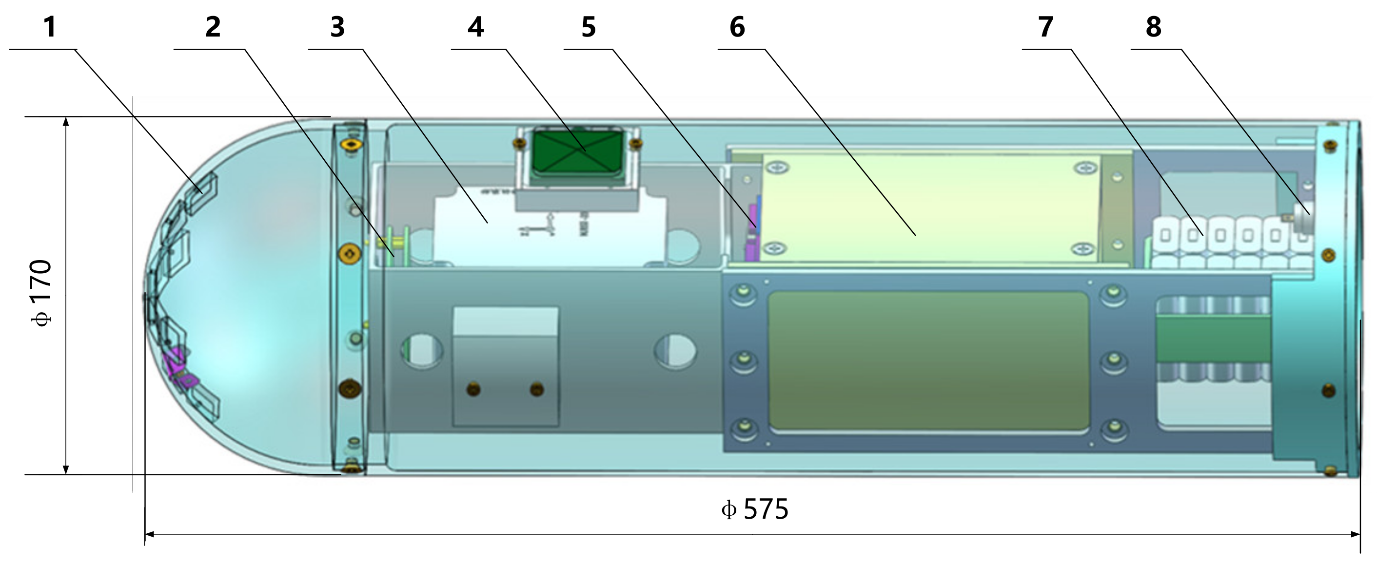
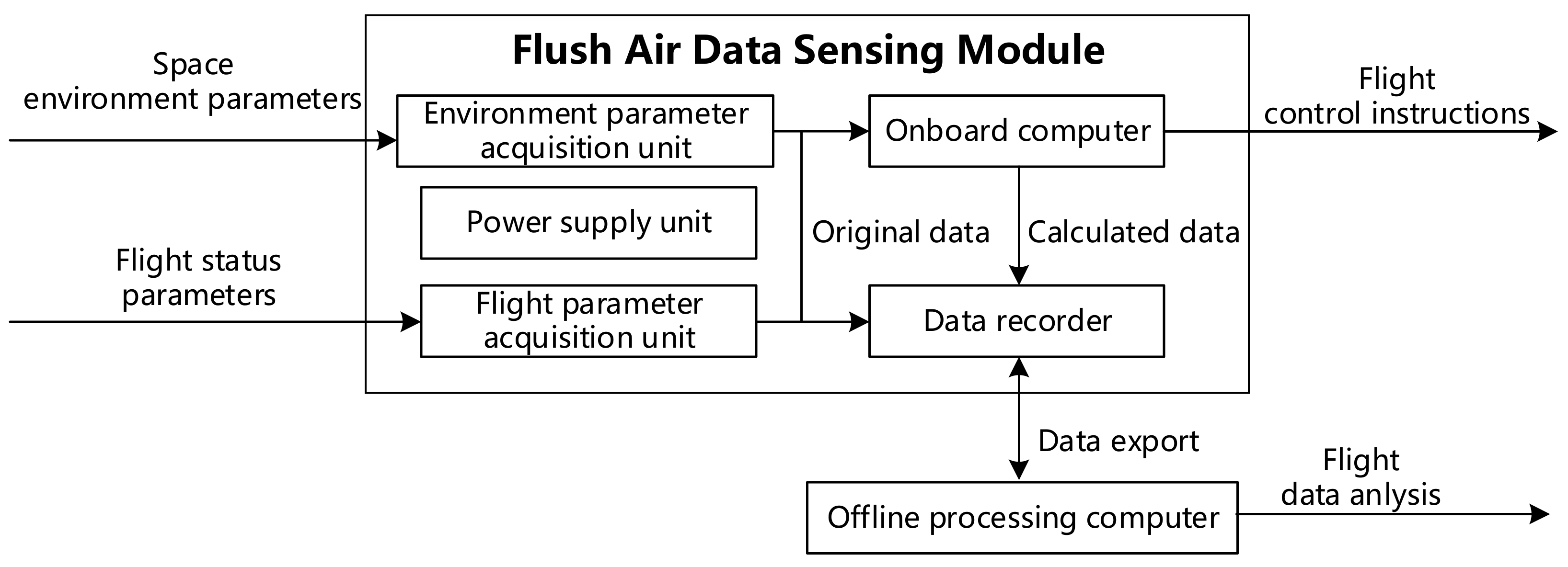
2.1. Hardware Structure

The designed flush air data sensing module adopts a hemispherical head and a cylindrical body scheme (as shown in Figure 2). The head shape can be changed into conical, oval, parabolic, double curved and other shapes according to the actual flight conditions.
The flush air data sensing module is mainly composed of nine pressure sensors, an onboard computer, integrated satellite navigation and inertial devices, a data recorder, a battery pack, and the necessary switches and electrical interfaces for data transmission among various components, etc. The internal structure is shown in Figure 3.
The onboard computer is the core component of the flush air data sensing module, which is used for online calculation of atmospheric parameters and to control the working logic of the system. It adopts a DSP chip + FPGA chip architecture, DSP is used for calculating the parameters, and FPGA is used for multiplexing serial ports to communicate with other electrical devices. The DSP model is a TMS320C6748 manufactured by Texas Instruments, Dallas, Texas, the U.S.A. with a main frequency of 300 MHz, and the FPGA model is an XC6SLX16CSG324 manufactured by Xilinx, San Jose, California, the U.S.A.
The data acquisition, processing and transfer speed of the module that can be mounted on aircraft systems have critical importance. The baud rate of communication from the data recorder to the onboard computer is set as 115,200 to ensure the whole system works normally. The frame frequency of data from the data recorder to the onboard computer is 64 Hz, which is fast enough for the calculations of the onboard computer.

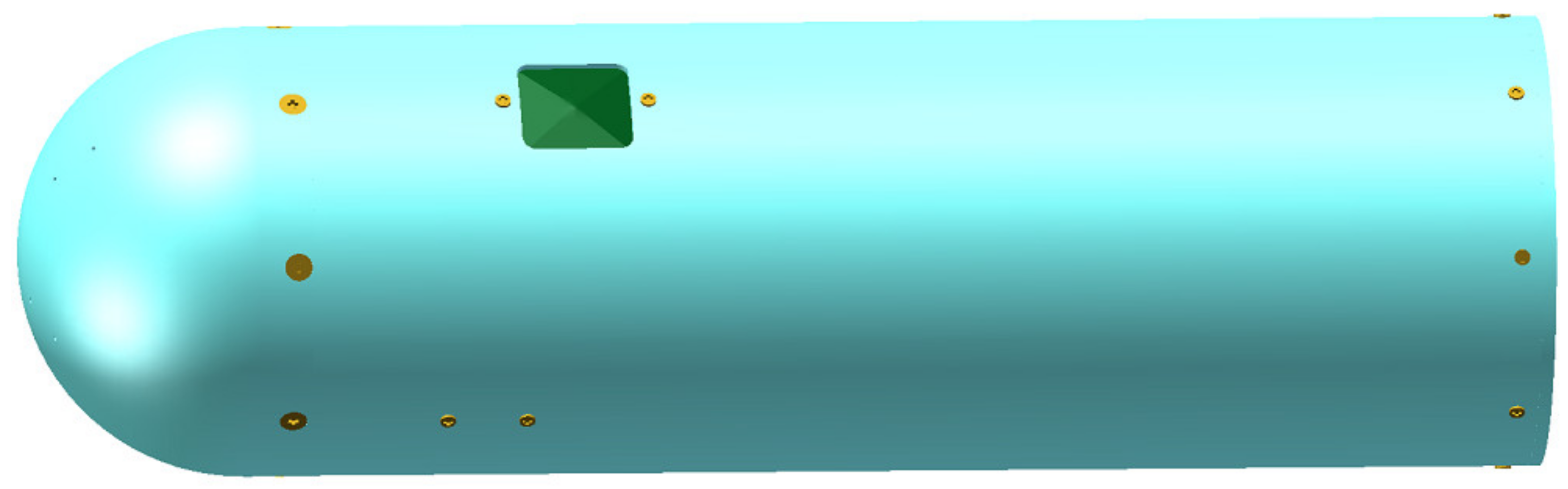
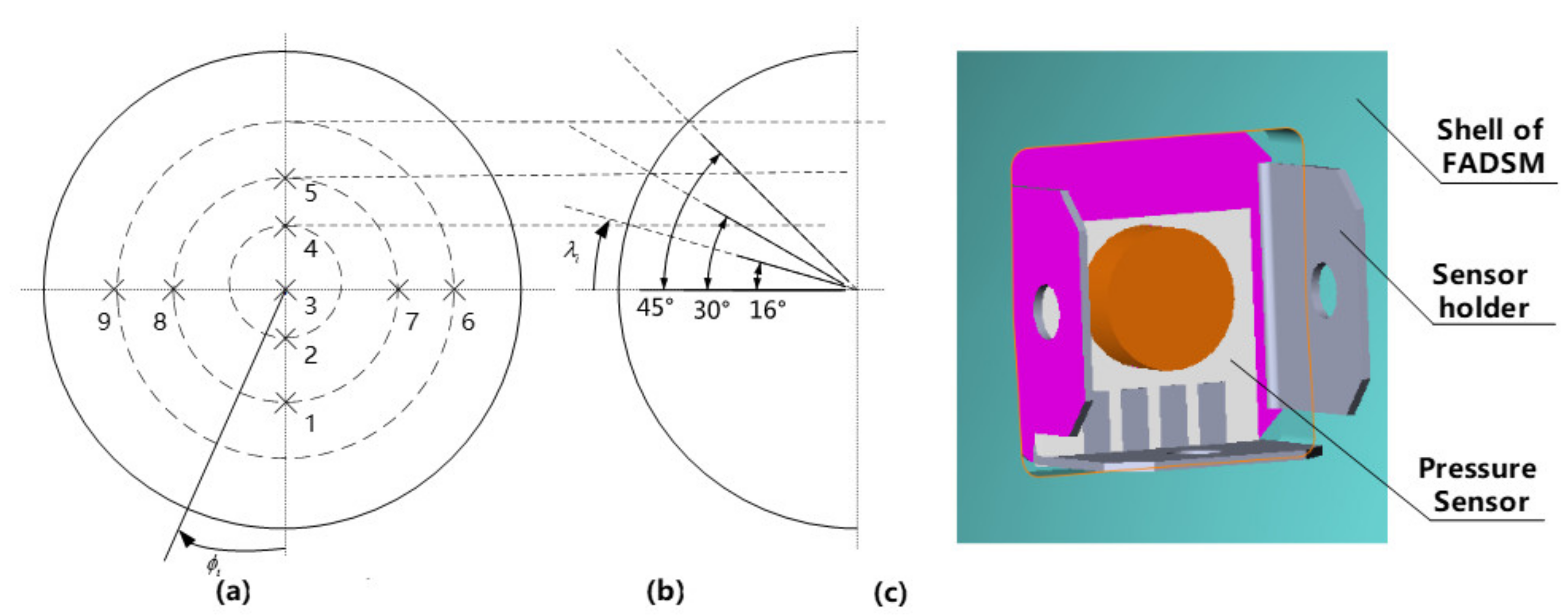
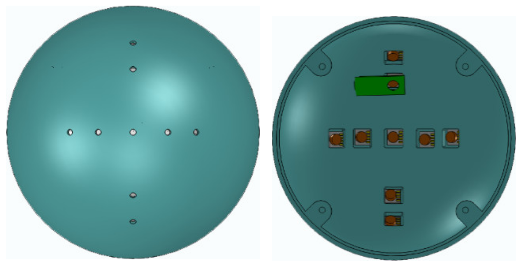
2.2. Pressure Sensors Layout Design

The head of the module adopts a hemispherical structure, and pressure sensors are installed in this head. The axis of a single sensor coincides with an angle normal to the hemispherical structure. The flush air data sensing module can be installed in front of a missile, so when the aircraft flies with different velocities and attitudes, the flow field near the pressure sensors will change according to the distributed position, then the angle of attack, angle of sideslip, dynamic pressure, static pressure and Mach number can be derived by an algorithm. Theoretically, the more pressure sensors there are, the more precise the calculation results will be, but because of the limited volume of the head of the flush air data sensing module, nine pressure holes are selected for the precision and convenience of the experiments. Using a flow field simulation, the layout position of the sensors is optimized as shown in Figure 4, where ϕ is defined as the circumference angle, (clockwise is positive when viewed from the direction of main view), and the zero degree line is down the direction of a plumb line as shown in Figure 4. λ is defined as the cone angle (clockwise is positive when viewed from the left view, and the horizontal line shown in Figure 4 is the zero degree line). Nine pressure sensors are used to measure the atmospheric pressure, and the serial numbers of these pressure sensors are shown in Figure 4. A close-up image of the holes drilled in the head of the module for pressure sensors to measure is also shown in Figure 4.

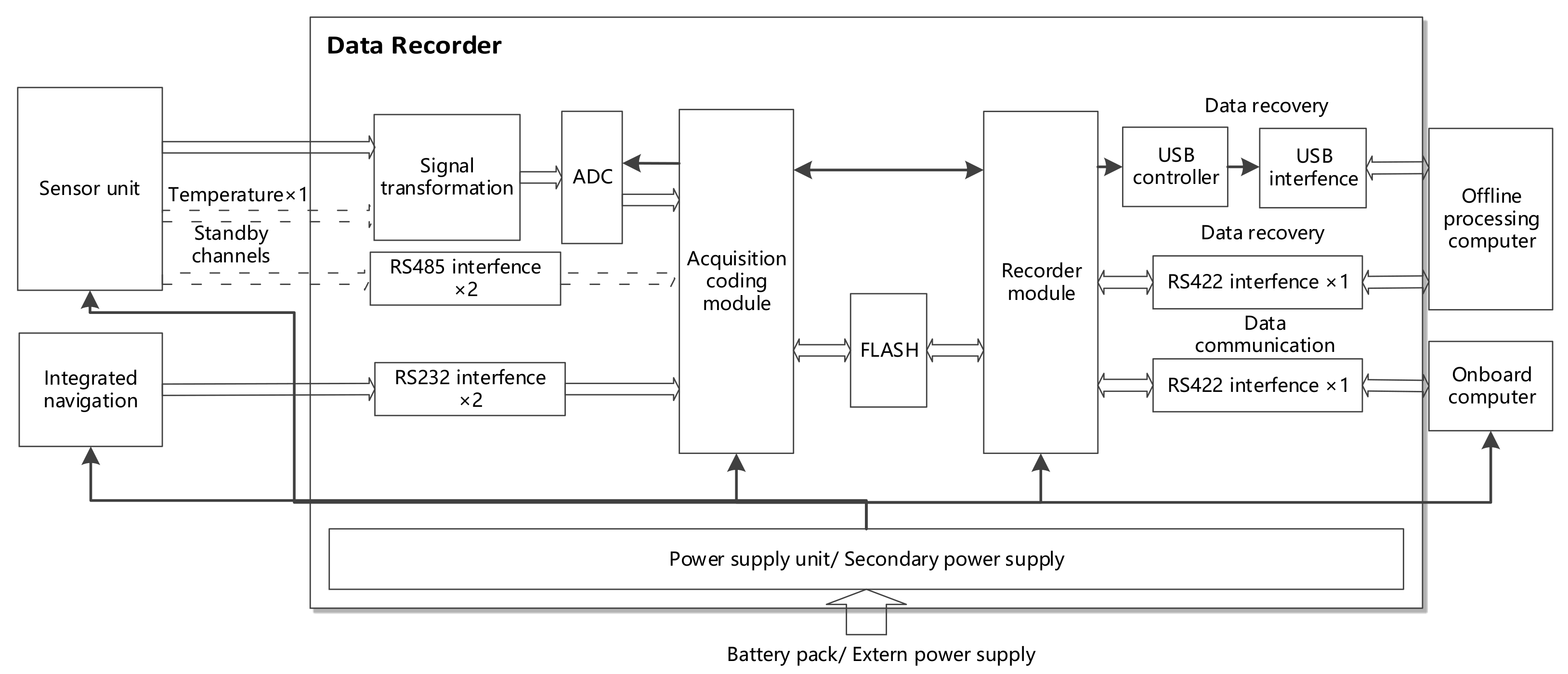
2.3. Electrical Scheme Design

The electrical scheme design focuses on the connections between the electrical equipment, data transmission interfaces and the overall scheme of the cable network. Specific models of sensors and other equipment can be selected for assembly according to the actual flight environment. The precision indicators should meet the specific flight mission needs. The schematic working diagram of the flush air data sensing module is shown in Figure 5, and the electrical connection schematic diagram is shown in Figure 6.
In Figure 5, the space environment parameters mainly include the atmospheric pressure and temperature, and the flight parameters mainly include the angular velocity, acceleration, position, speed, and attitude, etc. The environment parameter acquisition unit is composed of four or more pressure sensors and one or more temperature sensors. The more sensors, the higher calculation precision will be derived. Nine pressure sensors are selected here to get the required parameters. According to the specific mission, other types of sensors can be selected. The flight parameter acquisition unit comprises the integrated navigation system. The onboard computer is mainly used to calculate the angle of attack, angle of sideslip, dynamic pressure, static pressure and Mach number online with the measured information and generate the necessary flight control instructions. It can transmit calculated data and flight control instructions to other electrical equipment for specific missions. The data recorder can convert analog signals measured by the pressure sensors and temperature sensors into digital signals and transmit them to the onboard computer for calculation. It also stores the original data of flight status parameters, environment parameters and data calculated by the onboard computer. The power supply unit is a battery pack composed of lithium batteries. This battery pack supplies power to the data recorder, while the sensors, integrated navigation unit and onboard computer use secondary power provided by the data recorder to work. An offline processing computer can import data from the data recorder, which is used to analyze the flight process to optimize the guidance and control parameters. In the case of flight accidents, one can find the failure reasons and optimize the design of the guidance and control systems.
The data recorder is composed of an acquisition and storage circuit, signal conditioning circuit and RS422, RS232 isolation circuit, etc. It can adjust input sensor analog signals, and transform analog signals into digital signals. The data recorder can also store the data of the integrated navigation system and the onboard computer. All analog and digital signals are collected and programmed into a certain frame format and stored in a flash memory module. Meanwhile, the collected data is transmitted to the onboard computer online for display, analysis and processing in real time. When an experiment is finished, the data stored in the data recorder can be recovered by suitable data processing software, then it can be analyzed to determine the flight status.
The sensor unit is composed of nine pressure sensors. The temperature sensor is a standby unit with an analog channel, and two RS485 serial channels are in standby and not actually installed in the flush air data sensing module. A pressure sensor is composed of a sensitive device, a power supply circuit, a signal conditioning circuit, a filter circuit and an input and output interface. When a pressure sensor is powered, it outputs pressure with analog digitals for the data recorder to collect, convert, store and output in real time. When data is recovered from the data recorder, data processing software is used to analyze and calculate it.
The integrated navigation system mixes satellite signals and inertial signals together to get navigation information. The external plug-in integrated navigation unit is a J30J-25ZKP manufactured by Xi’an Lichuang Electronic Technology Co., Ltd., Xi’an, Hunan, China, which is connected with the data recorder through two RS232 serial interfaces to transmit the original inertial measurement and satellite measurement data. When it is powered, navigation information is transmitted to the data recorder through two RS232 serial interfaces for collection and storage. When an experiment is finished, data processing software is used to recover the integrated navigation data.
The external plug-in onboard computer is a J30J-25ZKP manufactured by Xi’an Lichuang Electronic Technology Co., Ltd., Xi’an, Hunan, China, which is connected with the data recorder through two RS422 serial interfaces. One RS422 serial interface is used to receive all kinds of data collected and compiled by the data recorder in real time. Another RS422 serial interface is available for expansion. The onboard computer calculates and analyzes the received data to get useful results, and the useful information is fed back to the data recorder through RS422 serial interface.
The independent external battery pack supplies power to the data recorder and provides +15 V voltage. The power supply unit of the data recorder includes a DC conversion module, which converts +15 V voltage into the required +5 V, ±12 V, +28 V voltages. It provides secondary power for the sensors (±12 V), integrated navigation system (+28 V) and the onboard computer (+5 V). The battery pack uses lithium batteries which can be charged and discharged repeatedly.
In the offline processing computer equipped with data processing software, which is used to store and recover data from the data recorder, the data format for recycling is .dat. Recovered data can be analyzed, calculated and expressed by figures. Calculated data can be exported as various formats for subsequent requirements.

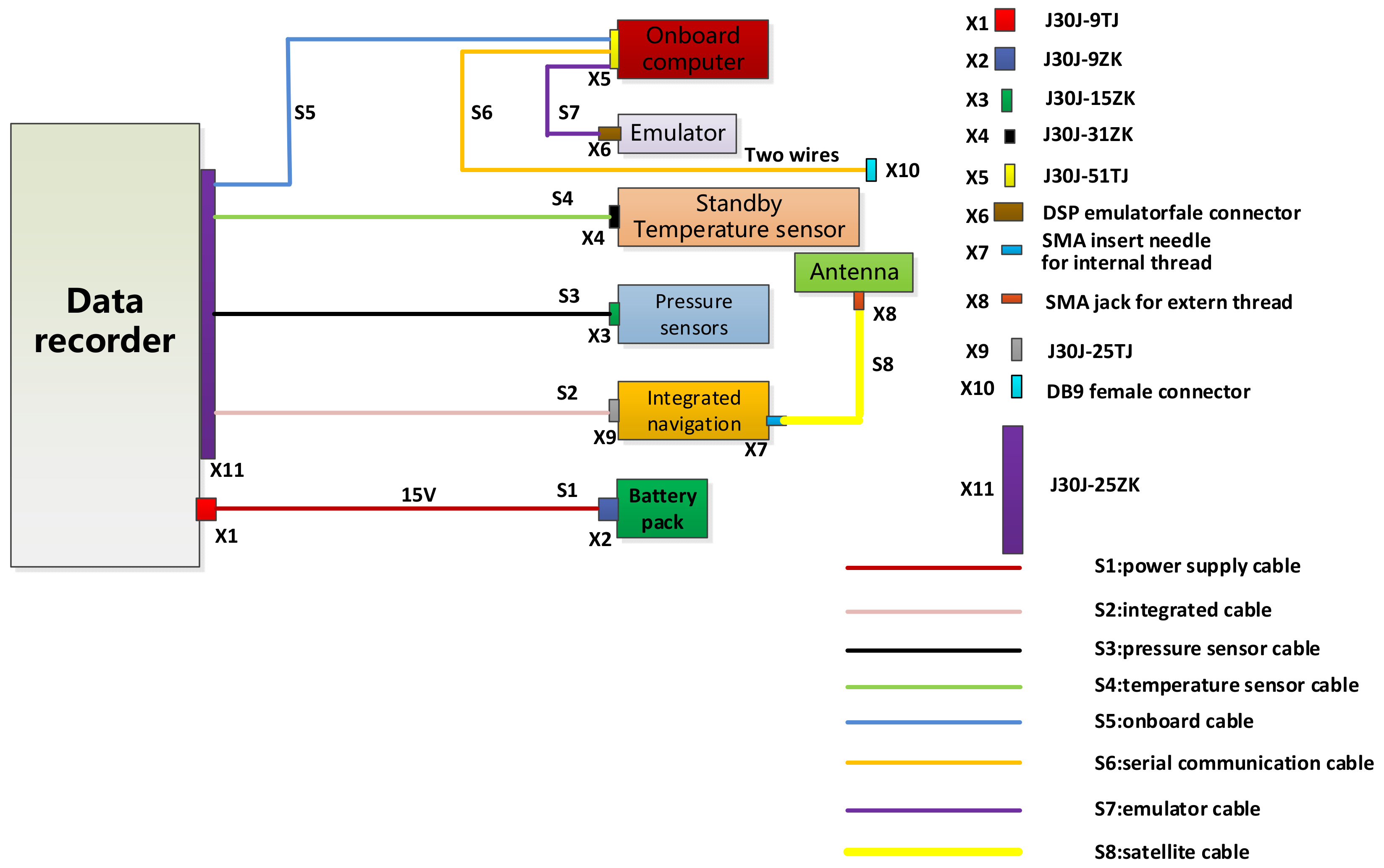
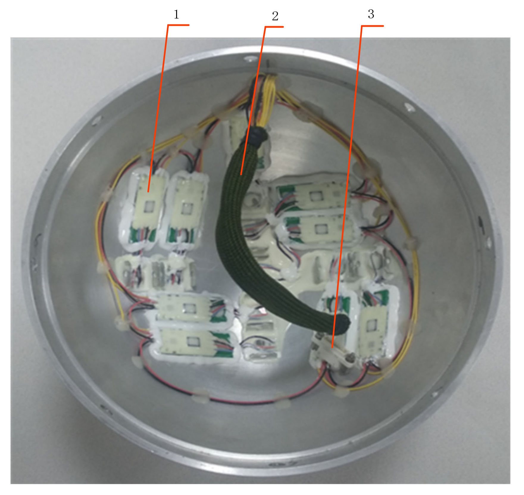
2.4. Cable Network Design

The cable network design of the proposed flush air data sensing module is shown in Figure 7. There are eight cables in the flush air data sensing module corresponding to ten electrical interfaces. X1–X10 represent the electrical wiring terminals and S1–S8 represent cables. TJ represents a plug insert pin, ZK represents a socket insert jack. The connectors shown in Figure 7 are models of cable outlet terminals, which are connected to each electrical device. The connector models of the electrical devices are not marked, and they are connected to connectors at the cable outlet terminals.

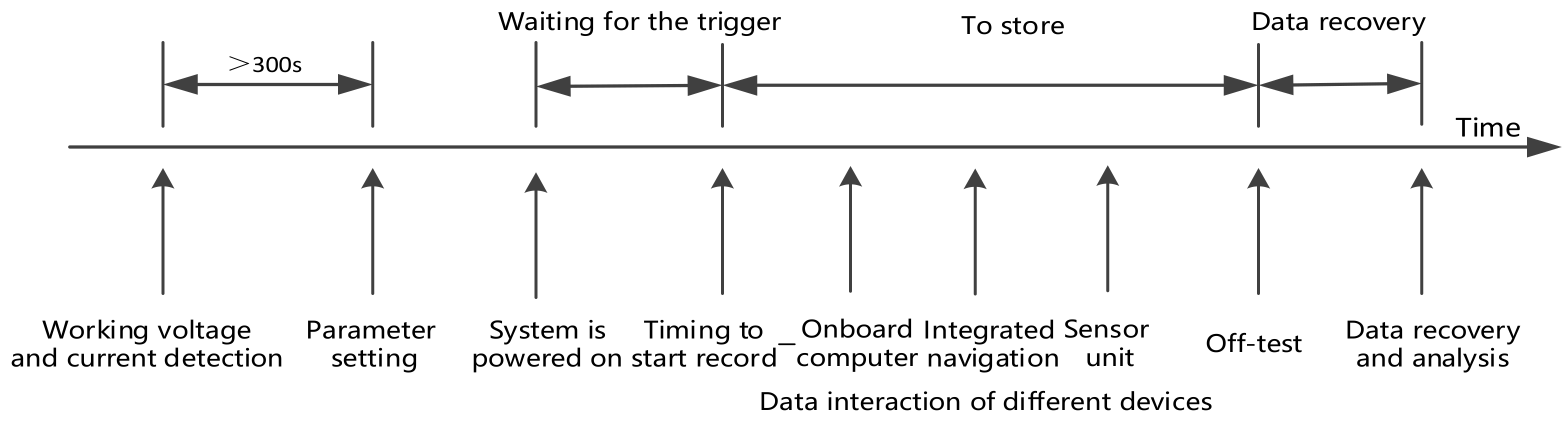
2.5. System Workflow

The workflow of the flush air data sensing module is as follows:
(1)
To check working voltage, current and set initial working parameters;
(2)
To start the timer and wait for its trigger;
(3)
When the timer triggers, the data recorder starts to collect and record data and supply power to the onboard computer, sensors and integrated navigation unit;
(4)
When the whole system begins to work, the pressure sensors measure the atmospheric pressure and the temperature sensor measures the atmospheric temperature with analog signals in real time. The data recorder will convert these analog signals from the sensors into digital signals, which are divided into two channels, one channel of data is connected to the onboard computer, while another channel of data is stored in the flash memory of the data recorder. The navigation system will get navigation information and transmit it to the onboard computer and data recorder. The onboard computer will mix data from the various devices together and calculate the angle of attack, angle of sideslip, dynamic pressure, static pressure, Mach number and so on, and the calculated data is transmitted to the data recorder for storage in real time;
(5)
When an experiment is finished, the data from the data recorder is recovered by the processing software in the offline processing computer. Recovered data can be analyzed to optimize the system iteratively. The system workflow is shown in Figure 8.

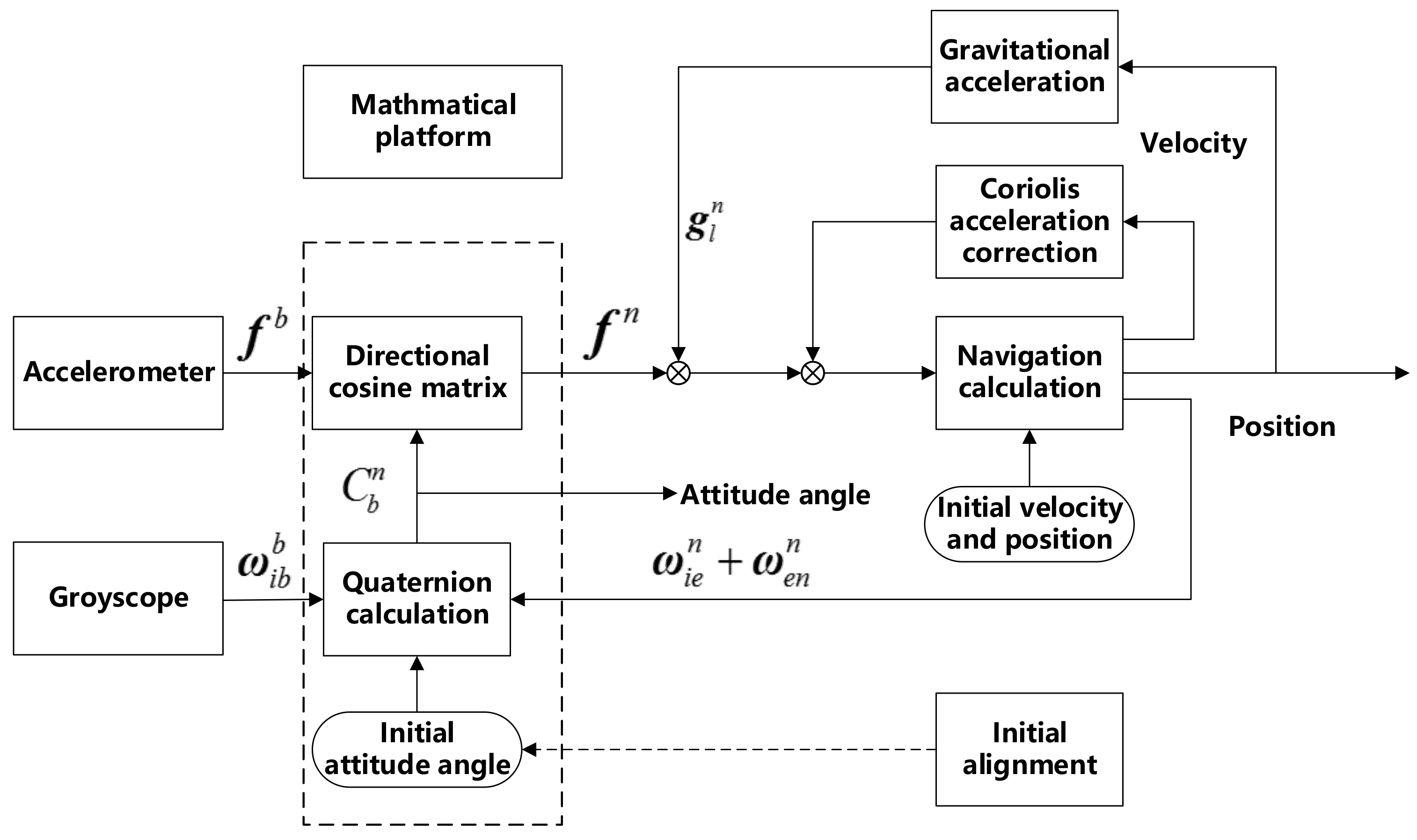
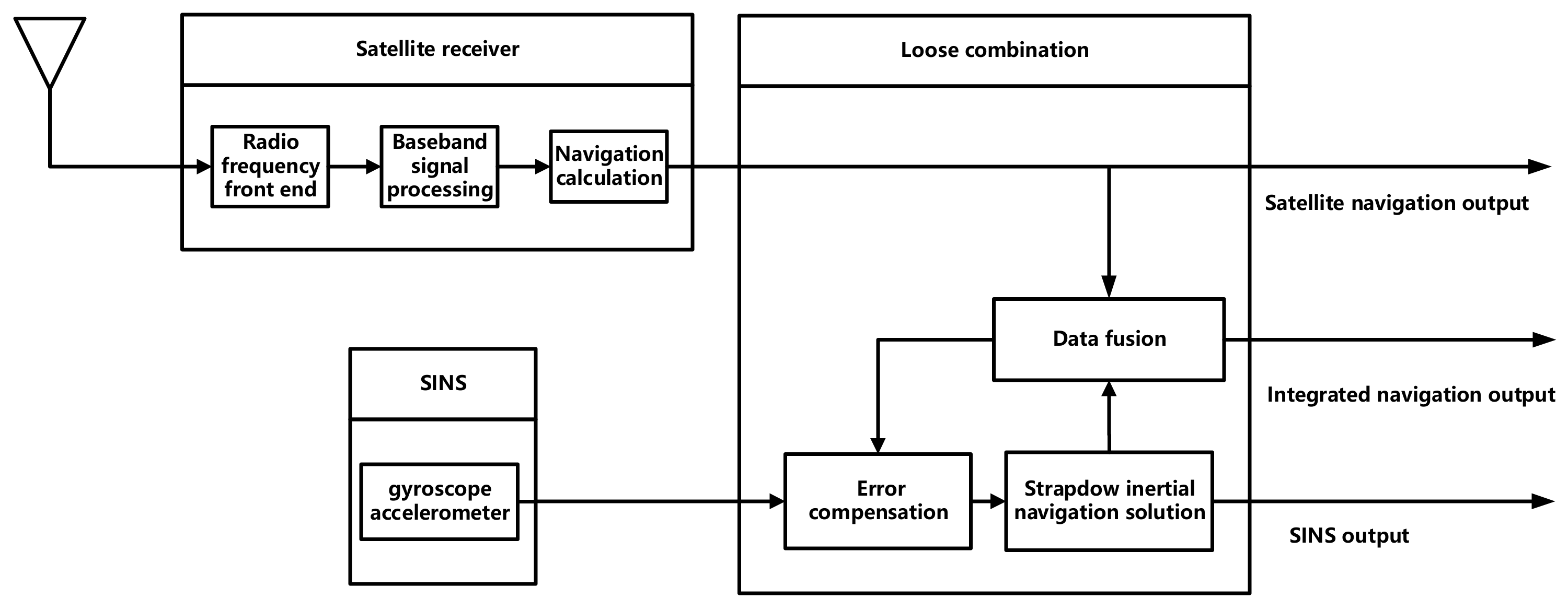
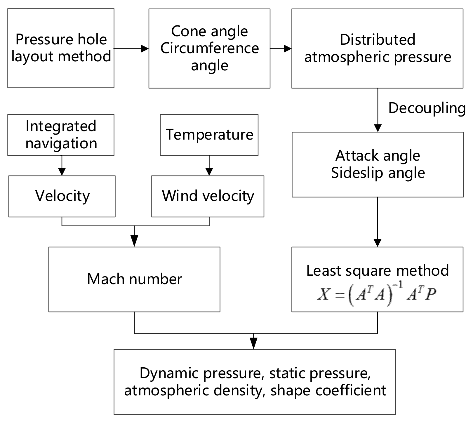
3. Atmospheric Parameter Calculation Algorithm

The installation position of the sensors is shown in Figure 9.
The measurement equation of a pressure sensor is:
p i = q c cos 2 θ i + ε sin 2 θ i + P
where, p i is the pressure value measured by the i-th pressure sensor, q c and P represent dynamic pressure and static pressure, respectively, ε represents the shape coefficient, which is affected by the flow compression, aerodynamic shape and other systems. It is usually regarded as a function of the angle of attack, angle of sideslip and Mach number f ε α , β , M a , and the precise function relationship should be determined by wind tunnel or flight tests. θ i represents the angle between the normal direction of the i-th pressure sensor and the local airflow velocity vector. It is known as the incoming flow incidence angle, which can be calculated from the local angle of attack and angle of sideslip:
cos θ i = cos ( α ) cos ( β ) cos ( λ i ) + sin ( β ) sin ( ϕ i ) sin ( λ i ) + sin ( α ) cos ( β ) cos ( ϕ i ) sin ( λ i )
where, λ i is the conical angle of the installation point of the i-th pressure sensor, which represents the angle between the normal direction of the pressure measuring hole and the central axis of the flush air data sensing module. ϕ i is the circumference angle of the installation point of the i-th pressure sensor, which represents the angle between the vertical center line in the main viewing direction to the axis of the pressure measuring hole direction. The units of λ i ,   ϕ i are rad. The definition of λ i ,   ϕ i is shown in Figure 4.
There is a definite function between dynamic pressure, static pressure and Mach number. Under subsonic conditions, the function can be solved by the isentropic flow rule. Under supersonic conditions, the adiabatic positive shock wave relation rule can be used to calculate the required parameters [20]. The specific equation is:
q c P = 1 + 0.2 M a 2 3.5 1 , M a 1 166.92 M a 2 M a 2 7 M a 2 1 2.5 1 , M a > 1

3.1. Calculation of the Angle of Attack and Angle of Sideslip

In the calculation process the input is the pressure value given by the pressure sensors. A three-point method is used to calculate the local angle of attack and angle of sideslip. According to the pressure values of three different pressure sensors, three measurement equations are established:
p i = q c 1 ε cos 2 θ i + q c ε + P p j = q c 1 ε cos 2 θ j + q c ε + P p k = q c 1 ε cos 2 θ k + q c ε + P
By combining these three equations and dividing the pressure value at any two pressure sensors by the difference, the following equation can be obtained:
p i p j p j p k = cos 2 θ i cos 2 θ j cos 2 θ j cos 2 θ k
Let τ i k = p i p k , τ j i = p j p i , τ k j = p k p j , to transfer the incident angle expression of Equation (2) into Equation (5), and take three points installed on a vertical line to realize decoupling of the local angle of attack and angle of sideslip, namely. We can then obtain:
cos ( α ) cos ( β ) cos ( λ j ) + s i n ( α ) c o s ( β ) s i n ( λ j ) 2 + τ j i cos ( α ) cos ( β ) cos ( λ k ) + s i n ( α ) c o s ( β ) s i n ( λ k ) 2 + τ k j cos ( α ) cos ( β ) cos ( λ i ) + s i n ( α ) c o s ( β ) s i n ( λ i ) 2 = 0
To expand the above equation, we know τ i k + τ j i + τ k j = 0 , so:
A = τ i k s i n 2 λ j + τ j i s i n 2 λ k + τ k j s i n 2 λ i B = τ i k cos λ j s i n λ j cos ϕ j + τ j i cos λ k s i n λ k cos ϕ k + τ k j cos λ i s i n λ i cos ϕ i
Thus, Equation (6) can be simplified as:
A ( tan 2 α 1 ) + 2 B tan α = 0
We can get α = 1 2 tan 1 A B .
According to the definition of incidence angle, then:
a i = cos α cos λ i + s i n α c o s ϕ i s i n λ i , b i = s i n ϕ i s i n λ i , and Equation (6) can be expressed as:
cos 2 β ( τ i k a j 2 + τ j i a k 2 + τ k j a i 2 ) + sin 2 β ( τ i k b j 2 + τ j i b k 2 + τ k j b i 2 ) + 2 sin β cos β ( τ i k a j b j + τ j i a k b k + τ k j a i b i ) = 0
Then:
A = τ i k b j 2 + τ j i b k 2 + τ k j b i 2 B = τ i k a j b j + τ j i a k b k + τ k j a i b i C = τ i k a j 2 + τ j i a k 2 + τ k j a i 2
Equation (9) can be simplified as:
A tan 2 β + 2 B tan β + C = 0
When A 0 , the following solution can be obtained:
tan β 1 , t a n β 2 = B A ± B A 2 C A
When A = 0 , it is easy to know tan β = C 2 B , and the value of the angle of sideslip can be obtained easily by using an inverse trigonometric function.

3.2. Calculation of the Mach Number

The Mach number is related to the sound velocity and the aircraft velocity:
M a = V V s
where V represents the aircraft speed, and V s represents the local sound velocity. The value of V can be measured by the integrated navigation system. The local sound velocity is related to the temperature which can be calculated by a temperature sensor:
V s = γ R T s
where, γ represents an adiabatic coefficient, equal to 1.4. R represents an air coefficient, which value is 287. R represents the atmospheric temperature. With all this the Mach number of an aircraft can be obtained by Equation (13).

3.3. Calculation of the Dynamic Pressure and Static Pressure

If the Mach number is obtained, Equation (3) and Equation (16) are combined. Putting the position information of pressure sensors, angle of attack and angle of sideslip calculated above into Equation (2), the incidence angle of each pressure measuring hole can be obtained. Then, the incidence angle can be put into Equation (1) to obtain the following equation:
p i = q c + P + q c ε 1 sin 2 θ i = 1 sin 2 θ i q c + P q c ε 1
The equation can be expressed as matrix form, A X = P , where:
A = 1 sin 2 θ 1 1 sin 2 θ n , X = X ( 1 ) X ( 2 ) , P = p 1 p n
The least squares solution can be obtained as: X = A T A 1 A T P .
Equations (3), (13) and (16) can be used to obtain dynamic pressure q c and the static pressure p .

3.4. Calculation of the Shape Coefficient and Atmospheric Density

From above equations, we can get:
t = X ( 1 ) X ( 2 ) = q c + P q c ε 1
This equation can be expressed as:
q c P = 1 t ε 1 1
According to the dynamic pressure q c , the static pressure p and the temperature t , the shape coefficient ε can be obtained.
The function between dynamic pressure q c and aircraft velocity V is:
q c = 1 2 ρ v 2
where ρ is the atmospheric density, then the atmospheric density ρ can be calculated as:
ρ = 2 q c V 2

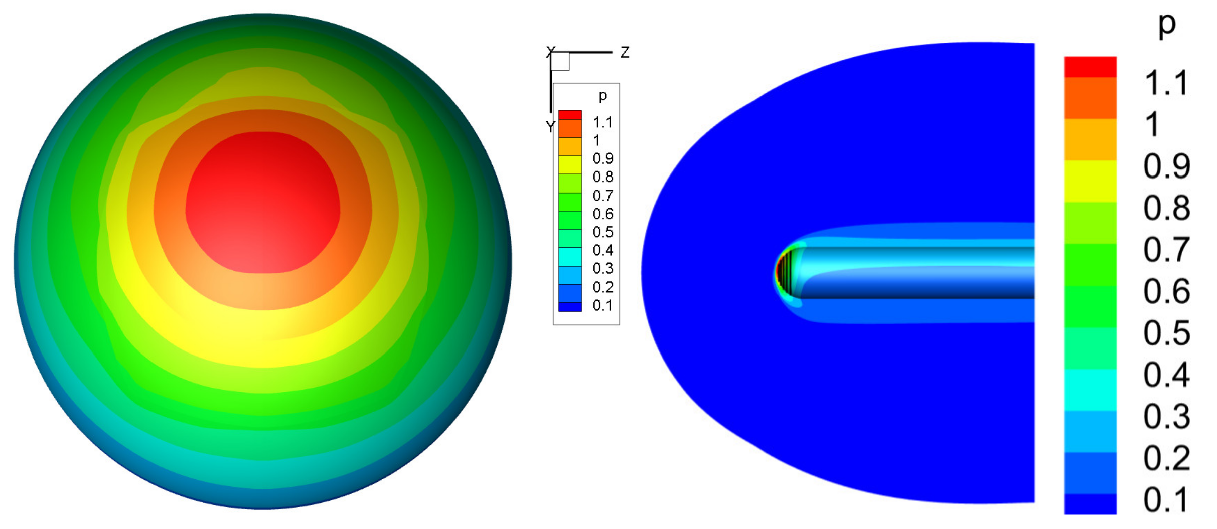
4. Flow Field Simulation Analysis

In order to realize decoupling between the angle of attack and angle of sideslip with convenient calculation, pressure sensors 1, 3 and 5 are used to calculate the angle of attack, and pressure sensors 6, 3 and 9 are used to calculate the angle of sideslip. Pressure sensors 1-9 are used to calculate the dynamic pressure, static pressure, Mach number, atmospheric density and shape coefficient. p i represents the measured pressure data of the i-th pressure sensor, the following equation can be obtained according to Equation (7):
A = p 5 p 1 4 B = 3 ( p 1 2 p 3 + p 5 ) 4 α = 1 2 arctan ( p 5 p 1 3 ( p 1 2 p 3 + p 5 ) )
The following equation can be obtained according to Equation (10):
A = p 9 p 6 2 B = ( 2 p 3 p 6 p 9 ) cos α 2 C = ( p 6 p 9 ) cos 2 α 2
If A 0
β = arctan ( ( 2 p 3 p 6 p 9 ) cos α p 6 p 9 ± [ ( 2 p 3 p 6 p 9 ) cos α p 6 p 9 ] 2 + ( p 6 p 9 ) cos 2 α p 6 p 9 )
If A = 0
β = arctan ( ( p 6 p 9 ) cos α 2 ( 2 p 3 p 6 p 9 ) )
Flow field simulation software is used for the simulation analysis. The real angle of attack is set as −13°, the angle of sideslip is set as 0°, the Mach number is set as 5, the height is set as 40 km, the temperature sensor precision is 0.25 °C, the integrated navigation system precision is 0.12 m/s, and the pressure sensor precision is 1 kPa. All the above parameters are set as the input conditions. The flow field simulated pressure distribution is shown in Figure 10, and the calculated results are shown in Table 1. The simulation software is a mature module in which the initial parameters are set before delivery, so the mesh and computational settings don’t need to be revised in the software, we only input the flight status parameters according to requirements in the assumption that the simulation software procedure is right.
It can be seen from Table 1 that the Mach number, calculated angle of attack and angle of sideslip have high precision, while the calculated dynamic pressure, static pressure, atmospheric density and shape coefficient have low precision. According to reference [21], it is proved that deviation of three-point method for the flush air data sensing module itself is very small and can be ignored here through wind tunnel experiments. Because of the large deviation of the flow field simulation data, the calculated flight status of the flush air data sensing module differs greatly from the real value of the flow field. The simulated results can show the change rules of the proposed algorithm and the workflow of the flush air data sensing module, and provide a reference for prospective wind tunnel experiments and flight tests. The theoretical analysis can also provide a reference for the design of an experimental scheme.

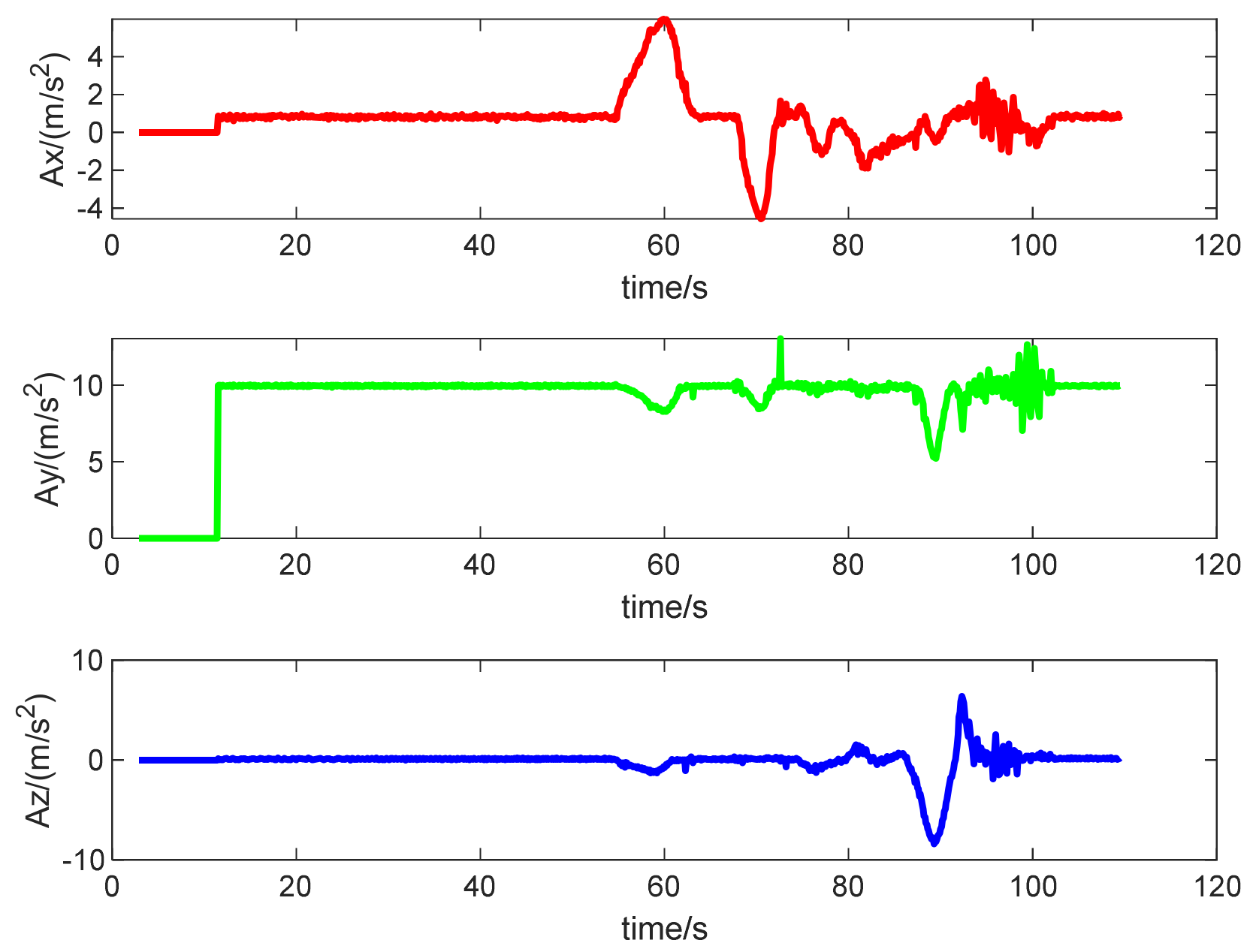
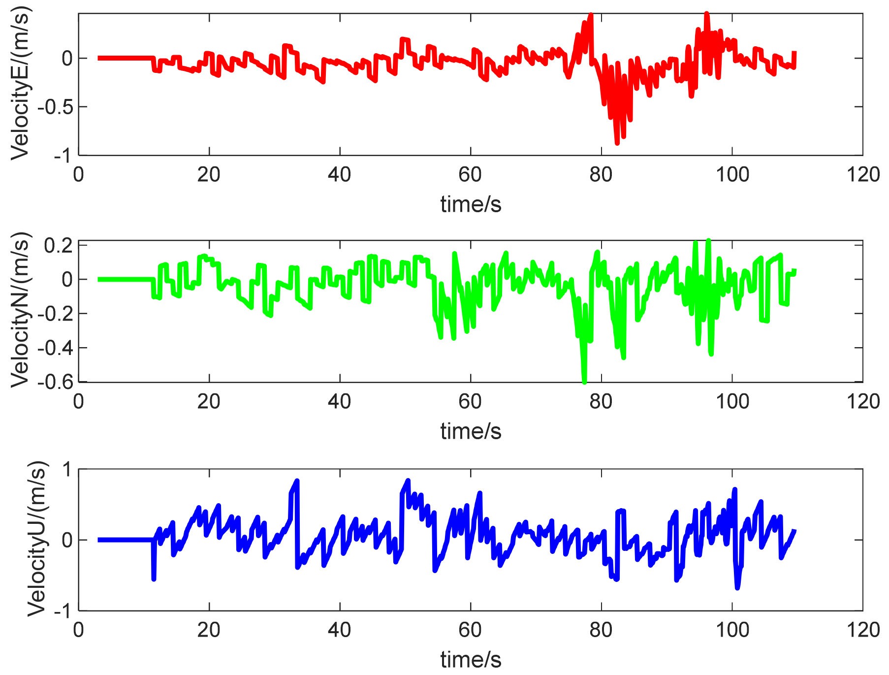
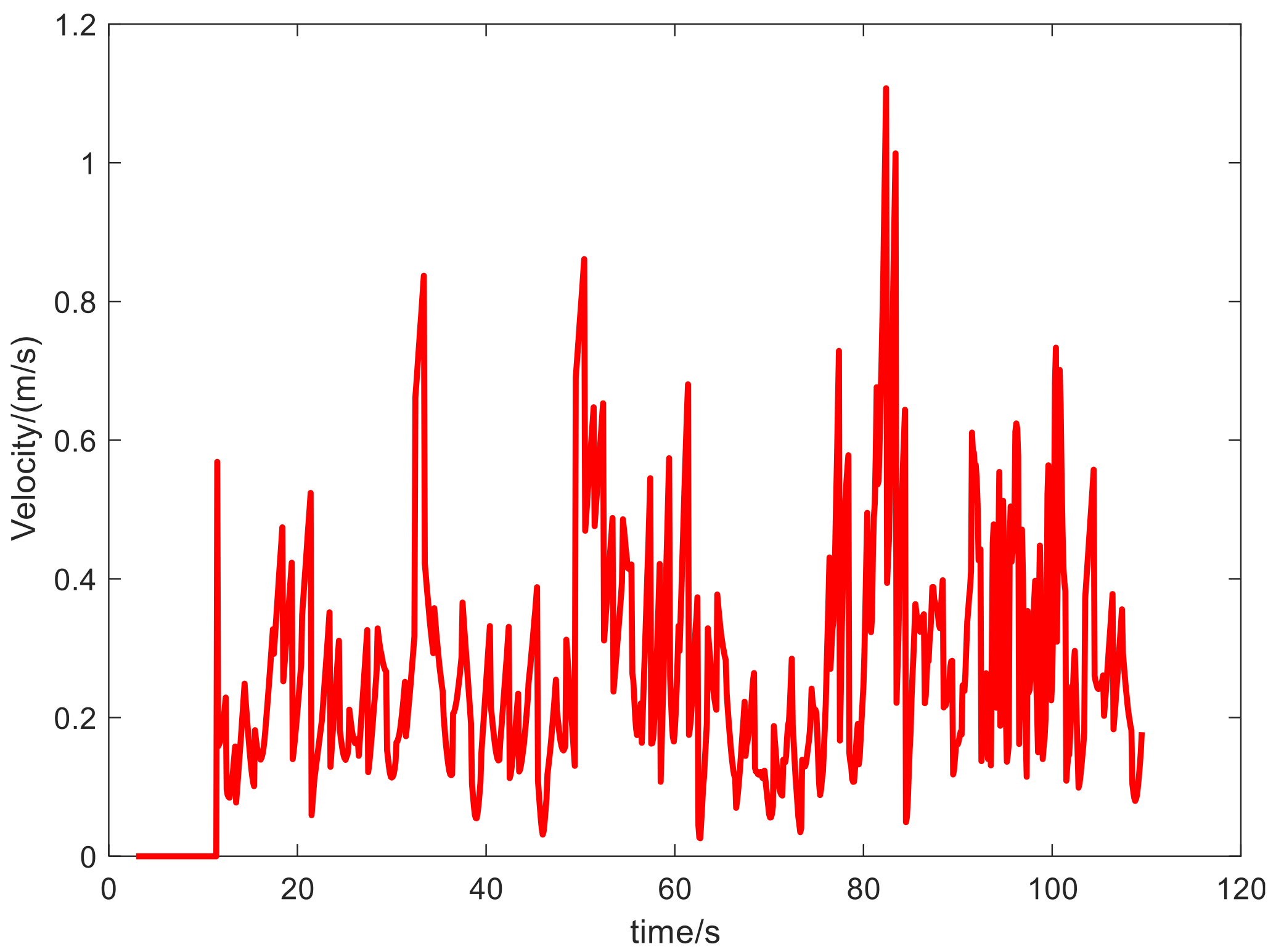
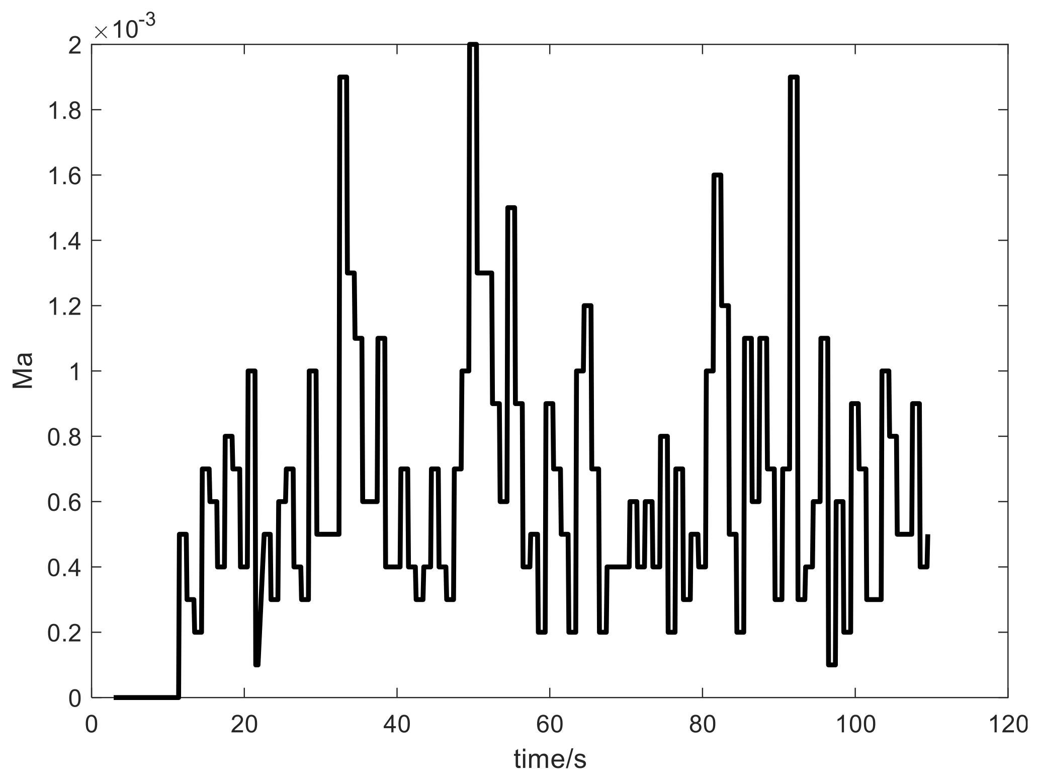
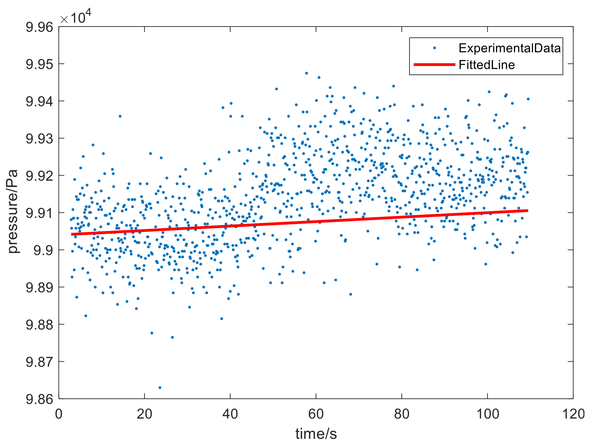
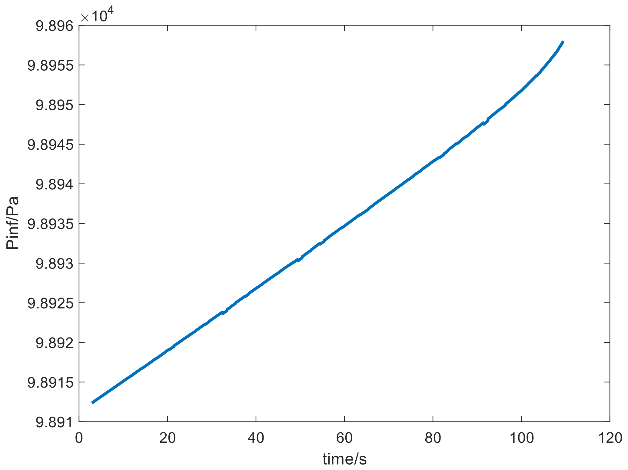
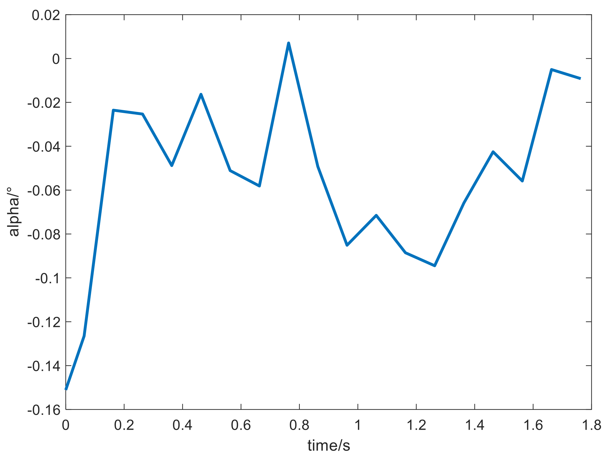
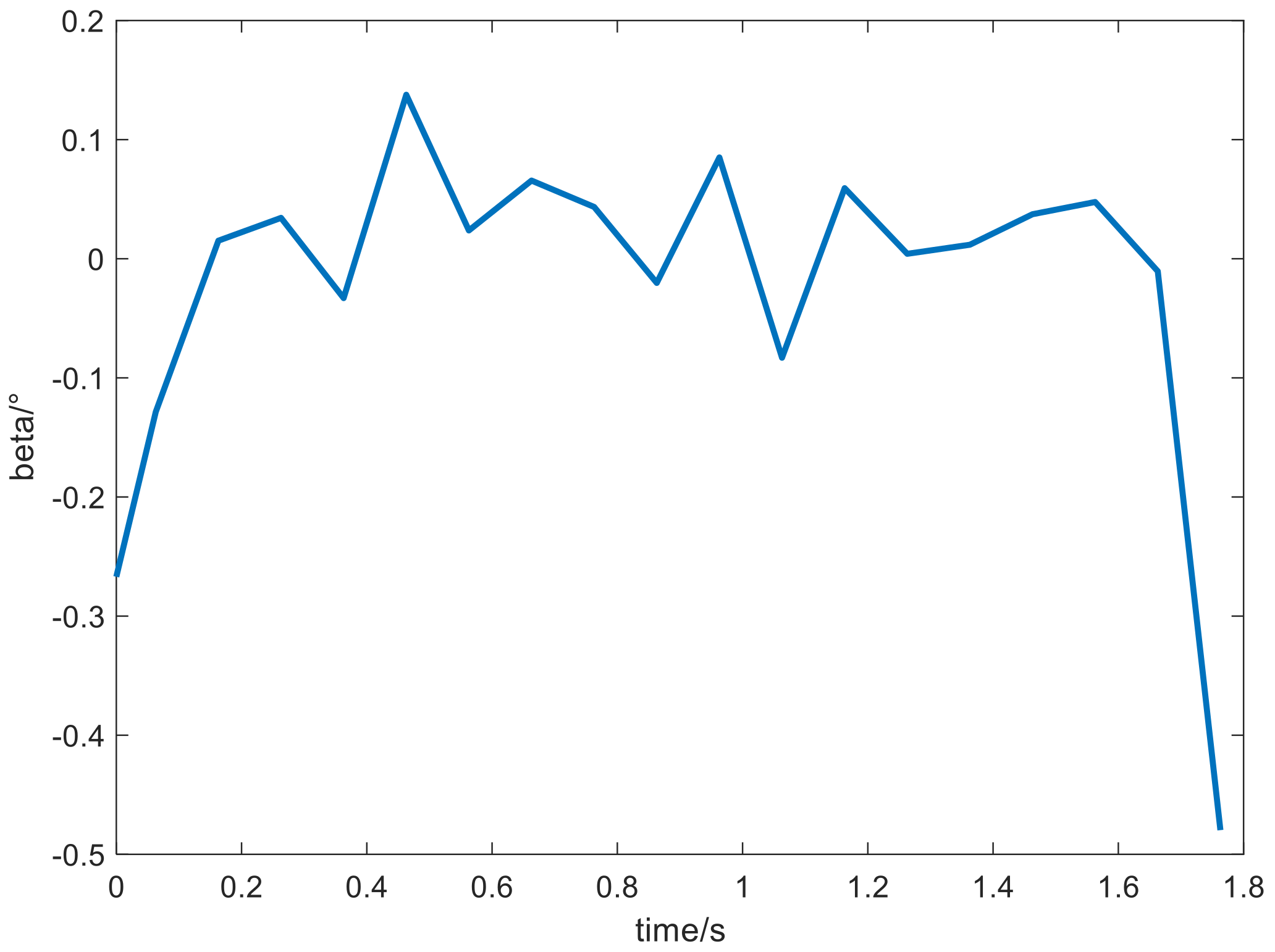
5. Experimental Verification

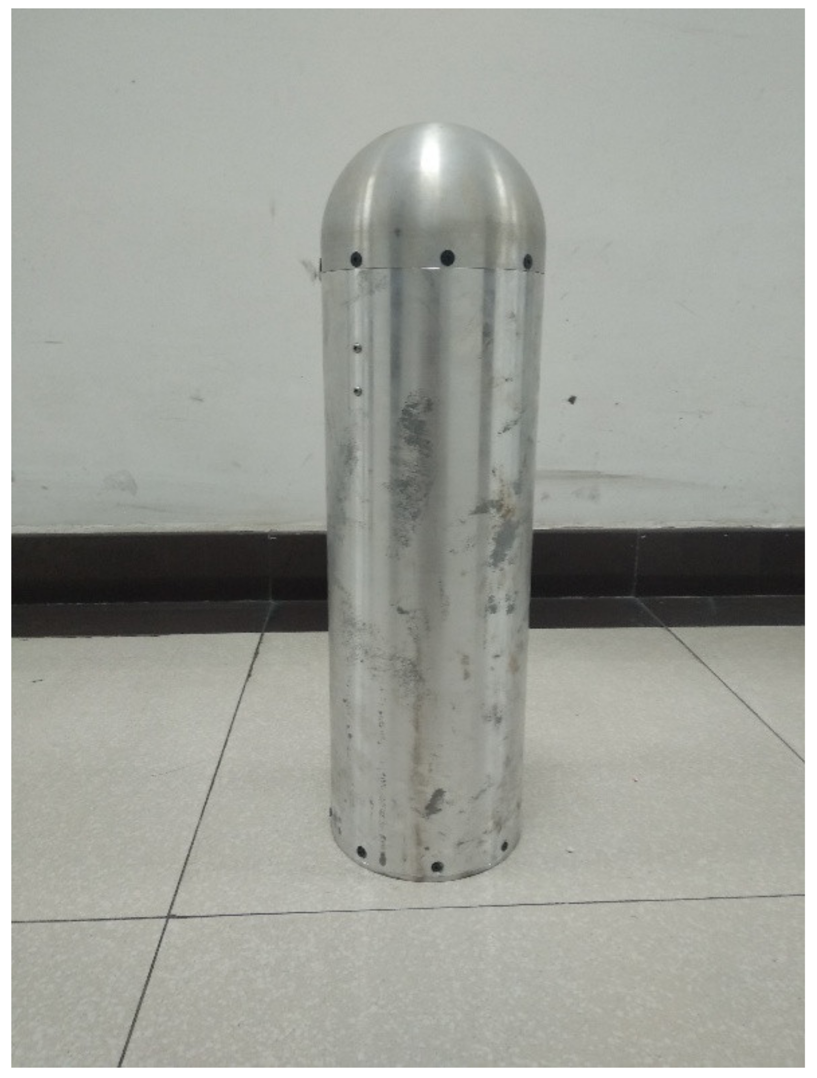
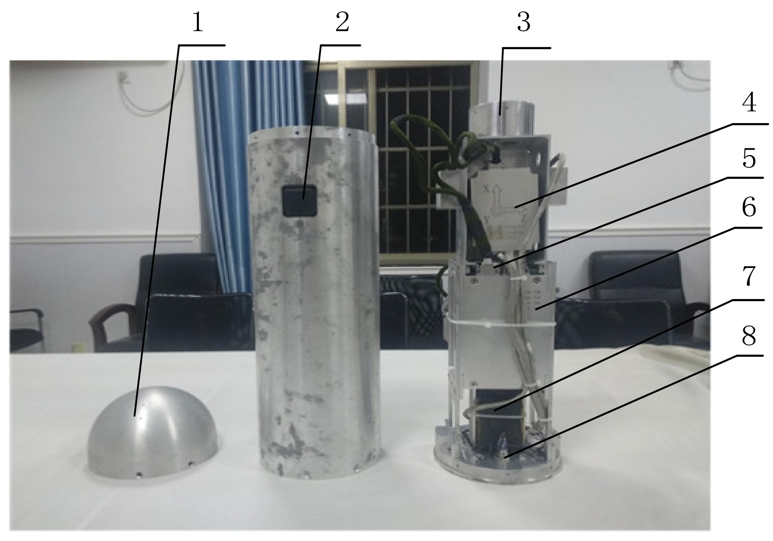
5.1. Physical Assembly

According to the design scheme, the proposed flush air data sensing module was manufactured, as shown in Figure 11.
There are nine pressure measuring holes on the head of the flush air data sensing module and each pressure measuring hole corresponds to a pressure sensor, as shown in Figure 12. A satellite antenna is connected to the integrated navigation system for receiving satellite signals. The integrated navigation unit adopts a combination of satellite and inertial device data. The inertial devices correspond to a strapdown micro-electromechanical system (MEMS), which contain MEMS gyroscopes and accelerometers. A loose combination solution is adopted between the satellite and inertial devices. The data recorder and pressure sensors work together, and analog data of the pressure sensors is converted into digital data by the data recorder. The onboard computer calculates the flight parameters online with the measured data. The electrical equipment have electrical interfaces and use data cables to communicate with each other. A battery pack supplies power to the whole system, and the system switch decides if the whole system will work or not. The schematic calculation diagram of the strapdown inertial navigation is shown in Figure 13. Integrated navigation using the loose combination between satellite and inertial device data is shown in Figure 14.

5.2. Test Workflow

In the designed overall scheme, the sensor unit include pressure sensors and temperature sensors, whereby pressure sensor data can be used for calculating the angle of attack and angle of sideslip directly, and temperature sensor data can be used for calculating the sound velocity, the integrated navigation system can be can be used for calculating the aircraft velocity, and the combination between a temperature sensor and the integrated navigation unit can be used for calculating the Mach number. The dynamic pressure and static pressure can be calculated by combination of the pressure sensor, temperature sensor and integrated navigation data [22]. This calculation process is shown in Figure 15.
The angle of attack and angle of sideslip are two very important parameters of aircraft, as almost all aerodynamic coefficients are related to the angle of attack, angle of sideslip and Mach number. Thus will lead to stalling phenomena when the angle of attack is too large, which results in serious failure. For the calculation of atmospheric parameters, the angle of attack and angle of sideslip are the basis to solve other parameters, and the precision of other parameters is also related to the angle of attack and angle of sideslip. For the designed flush air data sensing module, the calculation of the angle of attack and angle of sideslip are given high priority. Pressure sensors and integrated navigation are installed in the manufactured flush air data sensing module, while the temperature sensor is a reserved channel and has not been installed in the present version.
Pressure and velocity data are derived from measurements, while the atmospheric temperature is derived from a standard atmospheric calculation equation instead of a measurement. Taking measured data to verify if the data communication of the flush air data sensing module is normal or not, the system workflow can be also verified, which provides a reference for prospective wind tunnel experiments and flight tests.

5.3. Static Calculation Test

The prototype flush air data sensing module is stationary on the ground, so the real angle of attack and angle of sideslip are zero. The atmospheric parameters are calculated based on navigation, temperature and pressure information, so the calculation precision and the performance of system can be evaluated. The precision of navigation equipment is high, so the measurement value of navigation equipment is considered as the true value, and the measurement errors of navigation equipment are ignored. Then, the navigation equipment is moved randomly on the ground to represent small disturbance data to evaluate whether the system works normally and whether the calculated results of the angle of attack and angle of sideslip diverge in the case of a small disturbance of the navigation equipment data. The acceleration, eastern velocity, northern velocity, upward velocity, velocity magnitude and Mach number are respectively shown in Figure 16, Figure 17, Figure 18 and Figure 19. The hardware attributes of the flush air data sensing module have critical importance, while the sample rate, bandpass and the method to avoid aliasing and protection of recording data from external noise have been considered by the manufacturers of hardware, so the sample quality has been tested before delivery. When the experiments are carried out on the ground, the system works normally, so the parameters detailed above don’t need to be considered.
In Figure 16, the abscissa represents time and the ordinate represents the triaxial acceleration. At the beginning, the whole system has not completed initialization, so it is out of working state and the triaxial acceleration is zero. When the whole system is powered, the integrated navigation is not completely horizontal, so the gravity acceleration produces components in three axes. The magnitude of acceleration is about 9.8 m/s2, so the integrated information works normally. Then, experiments are carried out on the ground to control the flush air data sensing module’s movements as planned. The acceleration measured is consistent with the actual motion.
In Figure 17, the abscissa represents time and the ordinate represents the triaxial velocity. The integrated navigation unit integrates accelerometer data and combines it with satellite velocity data to get the integrated velocity. The velocity of the integrated navigation system is consistent with the actual motion.
In Figure 18, the abscissa represents time and the ordinate represents velocity. The variation curve of velocity with time is obtained by synthesizing the velocity vector, which is consistent with the actual motion.
In Figure 19, the abscissa represents time and the ordinate represents the Mach number. The temperature is obtained according to the standard atmosphere temperature, then the local sound velocity is obtained, so the curve of the Mach number changes with time can be obtained. Experimental results show that the proposed algorithm is feasible, and the Mach number of the flush air data sensing module can be calculated.
When experiments are carried out on the ground, the real angle of attack and angle of sideslip in motion are difficult to get, so the angle of attack and angle of sideslip are set as zero for a high quality standard value reference. The range of the pressure sensor is 200 kPa, and its precision is 1 kPa. This precision is too low for calculating the parameters. The measurement data will fluctuate around a real value with noise, and if the measurement data is fitted by a polynomial, it will have a small variance, and the data which is off the fitting curve will be considered as noise. The polynomial-fitting data is considered the real value, so the measurement noise is filtered. The digital data output of the pressure sensor is related to the one-time polynomial of the analog data input, so a one-time polynomial is used to fit the measured pressure data and filter out the influence of noise.
Pressure sensors 1, 3, 5 are mainly used to calculate the angle of attack. The measured pressure data fitting curve is shown in Figure 20, Figure 21 and Figure 22, a fitting curve comparison is shown in Figure 23, and the curve of the calculated angle of attack is shown in Figure 24. The calculation process of the angle of sideslip is the same as for the angle of attack, and the results are shown in Figure 25. Calculated dynamic pressure results are shown in Figure 26 and calculated static pressure results are shown in Figure 27.
As shown in Figure 21, Figure 22 and Figure 23, the abscissa represents time and the ordinate represents the pressure value. ExperimentalData represents the measured data, while FittedLine represents the line fitted by a one-time polynomial. P1, p3, and p5 represent lines of three pressure sensors fitted by the one-time polynomial, respectively. It can be seen that p1 and p3 are relatively close. Theoretically, the angle of attack of the flush air data sensing module is zero, so p1 and p3 should be completely consistent. Because the precision of the pressure sensor is low, the actual data fluctuation is large. The fitting method itself also has errors, which leads to further deviation of the fitted lines.
Figure 24 shows the calculated angle of attack results. The abscissa represents time and the ordinate represents the calculated value of the angle of attack. The theoretical angle of attack is zero when the flush air data sensing module is put on the ground without motion, so the deviation of the calculated angle of attack is less than 1°, and the precision of the calculated angle of attack is relatively high. When the flush air data sensing module flies at high speed with an actual specific angle of attack, the pressure measured by the distributed position of different pressure sensors is certain and the deviation is relatively stable, which allows us to obtain higher calculation precision by analysis. The calculated results are related to the algorithm itself, sensor precision, sensor installation position and assembly precision, etc., so calibration should be carried out before a flight to obtain higher calculation precision.
Figure 25 shows the calculated angle of sideslip results. The abscissa represents time, and the ordinate represents the calculated value of the angle of sideslip. When an experiment is carried out on the ground, the theoretical value of the angle of sideslip is zero, so the deviation of the calculated angle of sideslip is less than 0.5°. The calculated angle of sideslip results are related to the angle of attack, so the calculated precision of the angle of sideslip can be improved by improving the calculated precision of the angle of attack.
In Figure 26 and Figure 27, the abscissa represents time and the ordinate represents the pressure value. Qc represents the dynamic pressure, Pinf represents the static pressure. When the flush air data sensing module is on the ground without any motion, it can be seen that the dynamic pressure value changes very little, the maximum dynamic pressure value is less than 0.3 Pa, and the dynamic pressure change trend is consistent with the Mach number. The magnitude of the static pressure change is within 50 Pa, or about 1/10,000 relative to the standard atmospheric pressure, so noise interference is well suppressed by the proposed algorithm. The experimental results are consistent with the theoretical analysis, so the proposed algorithm and overall design verification scheme are well supported by the experimental data. Since there is a dynamic pressure term in the denominator of the calculation equation of the shape coefficient and atmospheric density, singular values will be generated while the dynamic pressure is very small, so the calculation of the shape coefficient and atmospheric density are not analyzed when the experiment is carried out on the ground. In the future, wind tunnel experiments and flight tests can be used to calculate the atmospheric density and shape coefficient, so as to obtain higher calculation precision.

5.4. Dynamic Calculation Test

When an aircraft is flying, the value derived from the pressure sensor will change in real time, and a dynamic measurement error will be generated. Dynamic calculation tests can evaluate whether the calculated angle of attack and angle of sideslip diverge with the fluctuation of pressure measurement data in the flight environment to ensure the normal status of the system. When an aircraft flies at zero angle of attack and zero angle of sideslip, the pressure at pressure measuring hole 3 is relatively large, and the pressure at other pressure measuring holes is relatively small. During the ground experiment, a large atmospheric pressure is injected into pressure measuring hole 3 to simulate flight status with zero angle of attack and zero angle of sideslip, so we can verify whether the calculated results are consistent with the theoretical analysis. Theoretically, when flying at zero angle of attack and zero angle of sideslip, the value of pressure sensor 3 should be greater than 1, 5, 6 and 9, which is less than twice that of other pressure sensors. It is reasonable to apply 1.6 times standard atmospheric pressure to pressure measuring hole 3.
Figure 28 shows the pressure data measured by pressure sensors 1, 3, 5, 6, 9, Figure 29 shows the calculated angle of attack and Figure 30 shows the calculated angle of sideslip.
In Figure 28, the abscissa represents time and the ordinate represents the pressure data measured by the pressure sensors. P1, p3, p5, p6, p9 represent the pressure values measured by pressure sensors 1, 3, 5, 6, 9, respectively. It can be seen that the maximum pressure measured by pressure sensor 3 is about 1.6 times that of pressure sensors 1, 5, 6, 9 after a large atmosphere pressure value is applied to pressure measuring hole 3. The applied atmosphere pressure varies continuously, it is increasing at first and then decreasing.
In Figure 29, the abscissa represents time and the ordinate represents the calculated angle of attack value. It can be seen that the calculated angle of attack value tends to zero, which is consistent with the theoretical analysis.
In Figure 30, the abscissa represents time and the ordinate represents the calculated angle of sideslip value. It can be seen that the calculated angle of sideslip value tends to zero, which is consistent with the theoretical analysis.

5.5. Engineering Application

The designed flush air data sensing module can be integrated into a single module with output electrical interfaces, which can be installed on the head of a missile, rocket, airplane and so on. Online calculations of the angle of attack, angle of sideslip, dynamic pressure, static pressure, Mach number, atmospheric density and shape coefficient can be transmitted to the guidance and control systems to develop the flight performance. A block diagram of an aircraft with a high performance guidance, navigation and control (GNC) system based on online calculated atmospheric parameters is shown in Figure 31. An aircraft based on the calculated atmospheric parameters and high performance GNC system will be used to complete a flight mission in the future.

6. Conclusions

Design and a verification scheme of a flush air data sensing module is proposed, and an overall composition scheme is designed in detail, simulation analysis and experimental verification are completed by proposed new algorithm with navigation information and temperature information. This work offers two main innovations:
(1)
The traditional three-point method is improved to integrate navigation information and temperature information for parameter calculation. The classical three-point algorithm uses pressure sensors and determines the shape coefficient through wind tunnel experiments to calculate the dynamic pressure, static pressure and Mach number. Wind tunnel experiments require high precision devices and costly operations. A new algorithm is proposed with pressure sensors, temperature sensors and an integrated navigation system to calculate the angle of attack, angle of sideslip, dynamic pressure, static pressure, Mach number, atmospheric density and shape coefficient. It is more convenient for calculating the required parameters with good real-time performance relative to the classic three-point algorithm. The proposed algorithm can obtain more useful parameters relative to the classic three-point algorithm with bright prospects. The proposed algorithm is verified by flow field simulation analysis and experimental tests, in which it can be seen that the simulated and experimental results are consistent with the theoretical analysis. It can provide a reference for prospective wind tunnel experiments and flight tests, and better calculation results can be obtained by the fusion of various data;
(2)
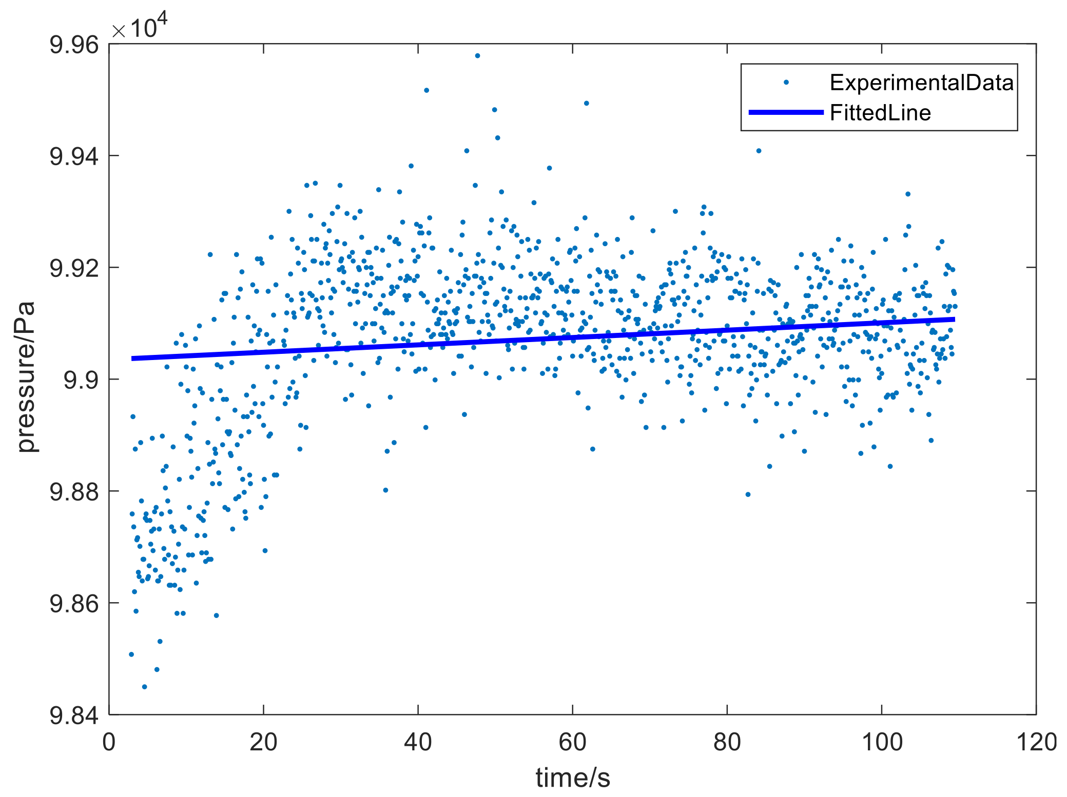
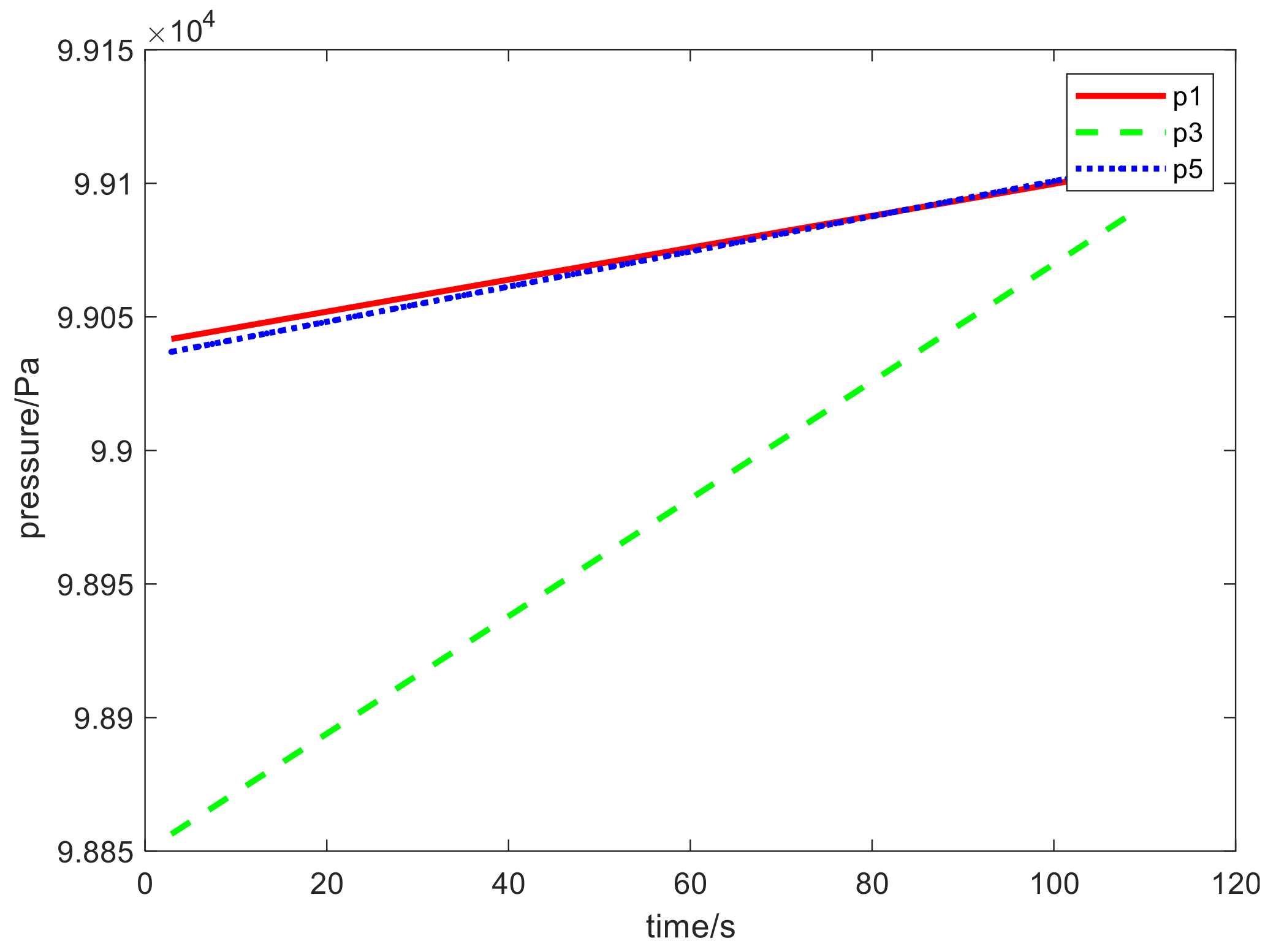
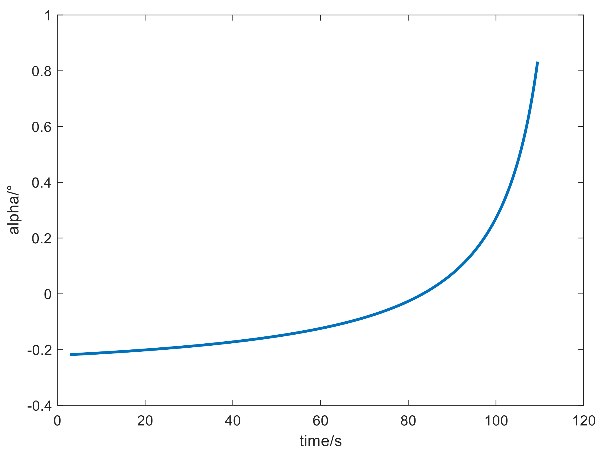
Proposing an intuitive function between the angle of attack, angle of sideslip and measured pressure. The analysis shows that a zero bias of the angle of attack is related to the difference between p1 and p5, and a zero bias of the angle of sideslip is related to p6 and p9, so pressure sensors 1, 5 are symmetrically distributed, and pressure sensors 6, 9 are also symmetrically distributed to reduce the zero bias in the flush air data sensing module. In order to improve the calculation precision, it is necessary to eliminate the zero bias as much as possible with analysis, so this has high significance for improving the installation precision of pressure sensors 1, 5, 6, 9. We can select high precision pressure sensors to reduce noise fluctuations and try to ensure consistency of fitted lines at symmetrical positions with measured data. The calculation precision of the angle of attack and angle of sideslip can be improved by reducing the zero bias, and the precision of other parameters will improve in the meanwhile, then the overall performance will be improved.
Flow field simulation analysis and experimental results can provide references for prospective wind tunnel experiments and flight tests. Different test methods can verify each other, so as to optimize the design scheme and obtain better calculation results. Online calculated results can be transmitted to a guidance and control system to evaluate the real-time flight status of aircraft and complete specific flight missions.

Author Contributions

Conceptualization, Z.J. and X.F.; methodology, X.F. and X.B.; software, X.F.; validation, Z.J., S.Z. and X.F.; formal analysis, S.Z.; investigation, S.Z.; resources, Z.J. and L.L.; data curation, X.F.; writing—original draft preparation, X.F.; writing—review and editing, Z.J.; visualization, X.F.; supervision, S.Z.; project administration, Z.J.; funding acquisition, L.L. All authors have read and agreed to the published version of the manuscript.

Funding

This research was funded by National Natural Science Foundation of China (Grant No.11802334).

Institutional Review Board Statement

Not applicable.

Informed Consent Statement

Not applicable.

Data Availability Statement

Not applicable.

Conflicts of Interest

The authors declare no conflict of interest.

References

  1. Khankalantary, S.; Sheikholeslam, F. Robust extended state observer-based three dimensional integrated guidance and control design for interceptors with impact angle and input saturation constraints. ISA Trans. 2020, 104, 299–309. [Google Scholar] [CrossRef] [PubMed]
  2. Zhang, H.X.; Gong, Z.F.; Cai, G.B. Reentry tracking control of hypersonic vehicle with complicated constraints. J. Ordnance Equip. Eng. 2019, 40, 1–6. [Google Scholar]
  3. Lyu, T.; Guo, Y.; Li, C.; Ma, G.; Zhang, H. Multiple missiles cooperative guidance with simultaneous attack requirement under directed topologies. Aerosp. Sci. Technol. 2019, 89, 100–110. [Google Scholar] [CrossRef]
  4. Tang, Y.; Zhu, X.; Zhou, Z.; Yan, F. Two-phase guidance law for impact time control under physical constraints. Chin. J. Aeronaut. 2020, 33, 126–138. [Google Scholar] [CrossRef]
  5. Palmer, C. The boeing 737 max saga: Automating failure. Engineering 2020, 6, 2–3. [Google Scholar] [CrossRef]
  6. Alvarez-Montoya, J.; Carvajal-Castrillón, A.; Sierra-Pérez, J. In-flight and wireless damage detection in a UAV composite wing using fiber optic sensors and strain field pattern recognition. Mech. Syst. Signal Process. 2020, 136, 106526. [Google Scholar] [CrossRef]
  7. Li, G.; Lee, H.; Rai, A.; Chattopadhyay, A. Analysis of operational and mechanical anomalies in scheduled commercial flights using a loga-rithmic multivariate Gaussian model. Transp. Res. C Emerg. Technol. 2020, 110, 20–39. [Google Scholar] [CrossRef]
  8. Jia, Q.; Hu, J.; He, Q.; Zhang, W. An Algorithm to Improve Accuracy of Flush Air Data Sensing. IEEE Sens. J. 2021, 21, 14987–14996. [Google Scholar] [CrossRef]
  9. Sankaralingam, L.; Ramprasadh, C. A comprehensive survey on the methods of attack angle measurement and estimation in UAVs. Chin. J. Aeronaut. 2020, 33, 749–770. [Google Scholar] [CrossRef]
  10. Marina, G.D.; Marcos; Haya. Attack angle and true airspeed failure sensor detection and recovery based on unscented Kalman filters for the alpha vehicle. In Proceedings of the 8th IFAC Symposium on Fault Detection, Supervision and Safety of Technical Processes, Mexico City, Mexico, 29–31 August 2012; pp. 1197–1202. [Google Scholar]
  11. Zeng, J.; Dou, L.; Xin, B. A joint mid-course and terminal course cooperative guidance law for multi-missile salvo attack. Chin. J. Aeronaut. 2018, 31, 1311–1326. [Google Scholar] [CrossRef]
  12. Zhao, Q.; Dong, X.; Song, X.; Ren, Z. Cooperative time-varying formation guidance for leader-following missiles to intercept a maneuvering target with switching topologies. Nonlinear Dyn. 2019, 95, 129–141. [Google Scholar] [CrossRef]
  13. Hua, Y.; Dong, X.; Li, Q.; Ren, Z. Distributed time-varying formation robust tracking for general linear multiagent systems with parameter uncertainties and external disturbances. IEEE Trans. Cybern. 2017, 47, 1959–1969. [Google Scholar] [CrossRef] [PubMed]
  14. Calia, A.; Denti, E.; Galatolo, R.; Schettini, F. Air data computa-tion using neural networks. J. Aircr. 2008, 45, 2078–2083. [Google Scholar] [CrossRef]
  15. Beck, R.; Karlgaard, C.; O’Keefe, S.; Siemers, P.; White, B.; Engelund, W.; Munk, M. Mars entry atmospheric data system modeling and algorithm development. In Proceedings of the AIAA Thermophysics Conference, San Antonio, TX, USA, 22–25 June 2009; pp. 1–21. [Google Scholar]
  16. Wang, P. Rbf neural network modeling and validation for fads system applied to the vehicle with sharp wedged fore-bodies. Phys. Gases. 2019, 4, 23–33. [Google Scholar]
  17. Liu, Y.; Xiao, D.B. Trade-off design of measurement tap configuration and solving model for a flush air data sensing system. Measurement 2016, 90, 278–285. [Google Scholar] [CrossRef]
  18. Chen, G.; Chen, B.; Li, P.; Bai, P.; Ji, C. Study on algorithms of flush air data sensing system for Hypersonic Vehicle. Procedia Eng. 2015, 99, 860–865. [Google Scholar] [CrossRef] [Green Version]
  19. Baumann, E.; Pahle, J.W.; Davis, M.C.; White, J.T. X-43A flush airdata sensing system flight-test results. J. Spacecr. Rocket. 2013, 47, 48–61. [Google Scholar] [CrossRef] [Green Version]
  20. Zhao, L. Research on Integrated Online Identification and Prediction Method of Missile Aerodynamic/Atmospheric Parameters. M.D. Thesis, National University of Defense Technology, Changsha, China, 2018; pp. 47–50. [Google Scholar]
  21. Li, Q.C.; Liu, J.F.; Liu, X.; Yang, Y.C.; Chen, J.C.; Tian, P.Z.; Yang, J.; Kang, H.B.; Zhu, S.M. The primary study of 3-point calculation method for the flush air data system. Acta Aerodyn. Sin. 2014, 32, 360–363. [Google Scholar] [CrossRef]
  22. Huang, Z.X. Research on Environmental Parameters Online Identification and Adaptive Control Method of Missile. M.D. Thesis, National University of Defense Technology, Changsha, China, 2017; pp. 15–16. [Google Scholar]
Figure 1. Designed flush air data sensing module.
Aerospace 08 00336 g001
Figure 2. Structure of the flush air data sensing module.
Aerospace 08 00336 g002
Figure 3. Internal structure of the proposed flush air data sensing module. 1-Pressure sensor unit, 2-Onboard computer, 3-Integrated navigation unit, 4-Satellite antenna, 5-Electrical interface, 6-Data recorder, 7-Battery pack, 8-System switch.
Aerospace 08 00336 g003
Figure 4. Distributed position of pressure sensors. (a) Front view, (b) Left view, (c) A close-up image of pressure measuring hole
Aerospace 08 00336 g004
Figure 5. Working schematic diagram of the flush air data sensing module.
Aerospace 08 00336 g005
Figure 6. Electrical connection schematic diagram of the flush air data sensing module.
Aerospace 08 00336 g006
Figure 7. Cable network of the flush air data sensing module.
Aerospace 08 00336 g007
Figure 8. Working flow of the flush air data sensing module.
Aerospace 08 00336 g008
Figure 9. Installation position diagram of the pressure sensors.
Aerospace 08 00336 g009
Figure 10. Pressure distribution diagram.
Aerospace 08 00336 g010
Figure 11. Physical picture of flush air data sensing module. 1-Pressure measuring hole, 2-Satellite antenna, 3-Onboard computer, 4-Integrated navigation, 5-Electrical interface, 6-Data recorder, 7-Battery pack, 8-System switch.
Aerospace 08 00336 g011
Figure 12. Physical diagram of pressure sensors. 1-Pressure sensors, 2-Data cables, 3-Plug-in.
Aerospace 08 00336 g012
Figure 13. Calculation schematic diagram of the strapdown inertial navigation system.
Aerospace 08 00336 g013
Figure 14. Integrated navigation using a loose combination between satellite and inertial device data.
Aerospace 08 00336 g014
Figure 15. Calculation process of the flush air data sensing module.
Aerospace 08 00336 g015
Figure 16. Measured triaxial acceleration data.
Aerospace 08 00336 g016
Figure 17. Measured integrated velocity data.
Aerospace 08 00336 g017
Figure 18. Variation curve of velocity with time.
Aerospace 08 00336 g018
Figure 19. Variation curve of Mach number with time.
Aerospace 08 00336 g019
Figure 20. Measured data and fitting curve of pressure sensor 1.
Aerospace 08 00336 g020
Figure 21. Measured data and fitting curve of pressure sensor 3.
Aerospace 08 00336 g021
Figure 22. Measured data and fitting curve of pressure sensor 5.
Aerospace 08 00336 g022
Figure 23. Comparison of pressure sensor fitting curves.
Aerospace 08 00336 g023
Figure 24. Calculated angle of attack results.
Aerospace 08 00336 g024
Figure 25. Calculated angle of sideslip results.
Aerospace 08 00336 g025
Figure 26. Calculated dynamic pressure results.
Aerospace 08 00336 g026
Figure 27. Calculated static pressure results.
Aerospace 08 00336 g027
Figure 28. Pressure data measured by pressure sensors 1, 3, 5, 6, 9.
Aerospace 08 00336 g028
Figure 29. Calculated angle of attack results.
Aerospace 08 00336 g029
Figure 30. Calculated angle of sideslip results.
Aerospace 08 00336 g030
Figure 31. Block diagram of an aircraft with high performance GNC system based on online calculated atmospheric parameters.
Aerospace 08 00336 g031
Table 1. Calculated parameters and real parameters of specific conditions.
ParametersReal ValueCalculated Value
Angle of attack−13°−13.714°
Angle of sideslip−0.66076°
Dynamic pressure5025.01021 Pa6543.43605 Pa
Static pressure287.144 Pa206.807 Pa
Mach number55.00263
Atmospheric density0.00399568 kg/m30.00520369 kg/m3
Shape coefficient0.011405870.03528756
Publisher’s Note: MDPI stays neutral with regard to jurisdictional claims in published maps and institutional affiliations.

